


Airfoil Optimization and Analysis Using Global Sensitivity Analysis and Generative Design


Abstract
1. Introduction
2. Numerical Model
2.1. Airfoil Parametrization
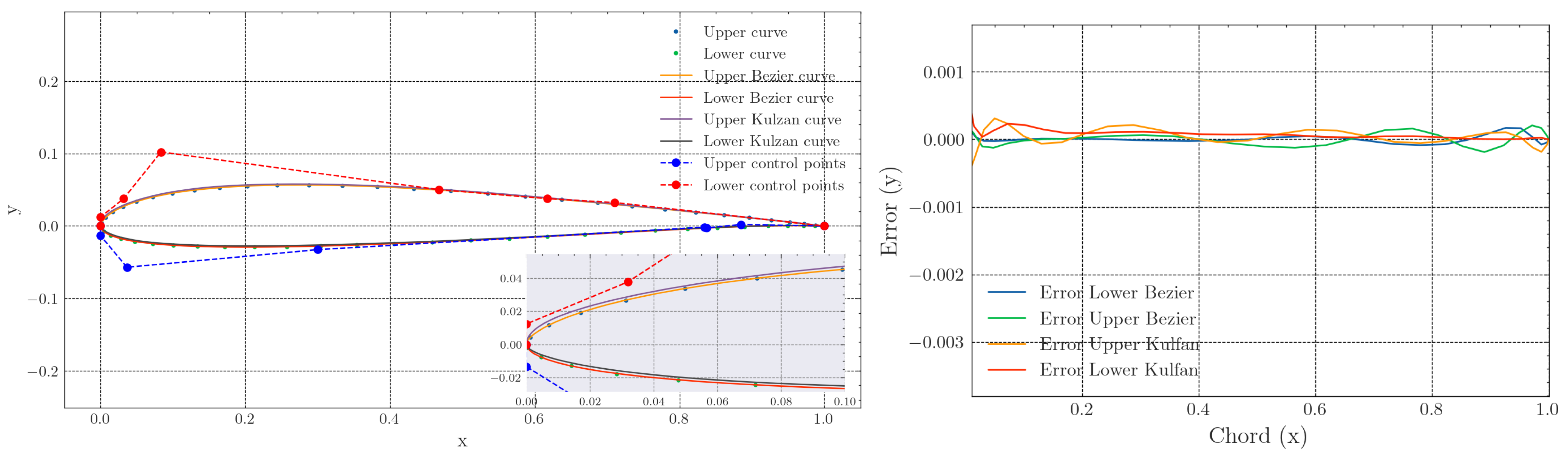
2.1.1. CST Method
2.1.2. Bézier Surface
2.2. Global Sensitivity Analysis
2.3. Generative Design
2.4. Particle Swarm
2.5. Case Study
3. Results
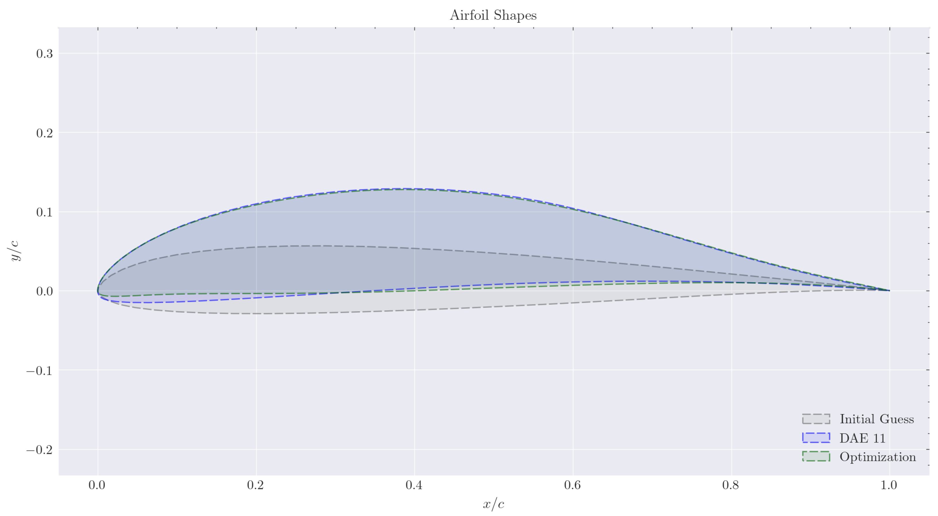
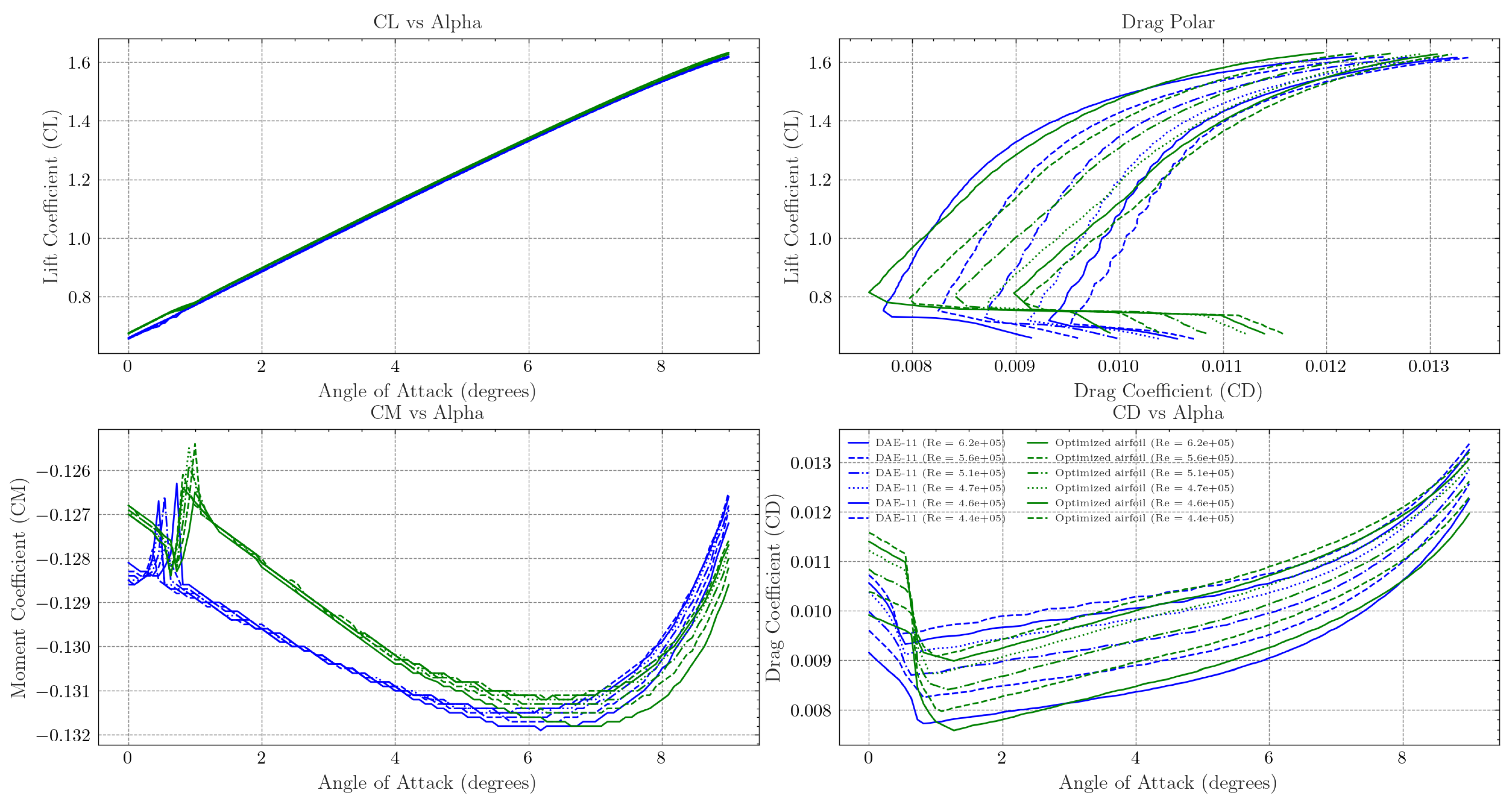
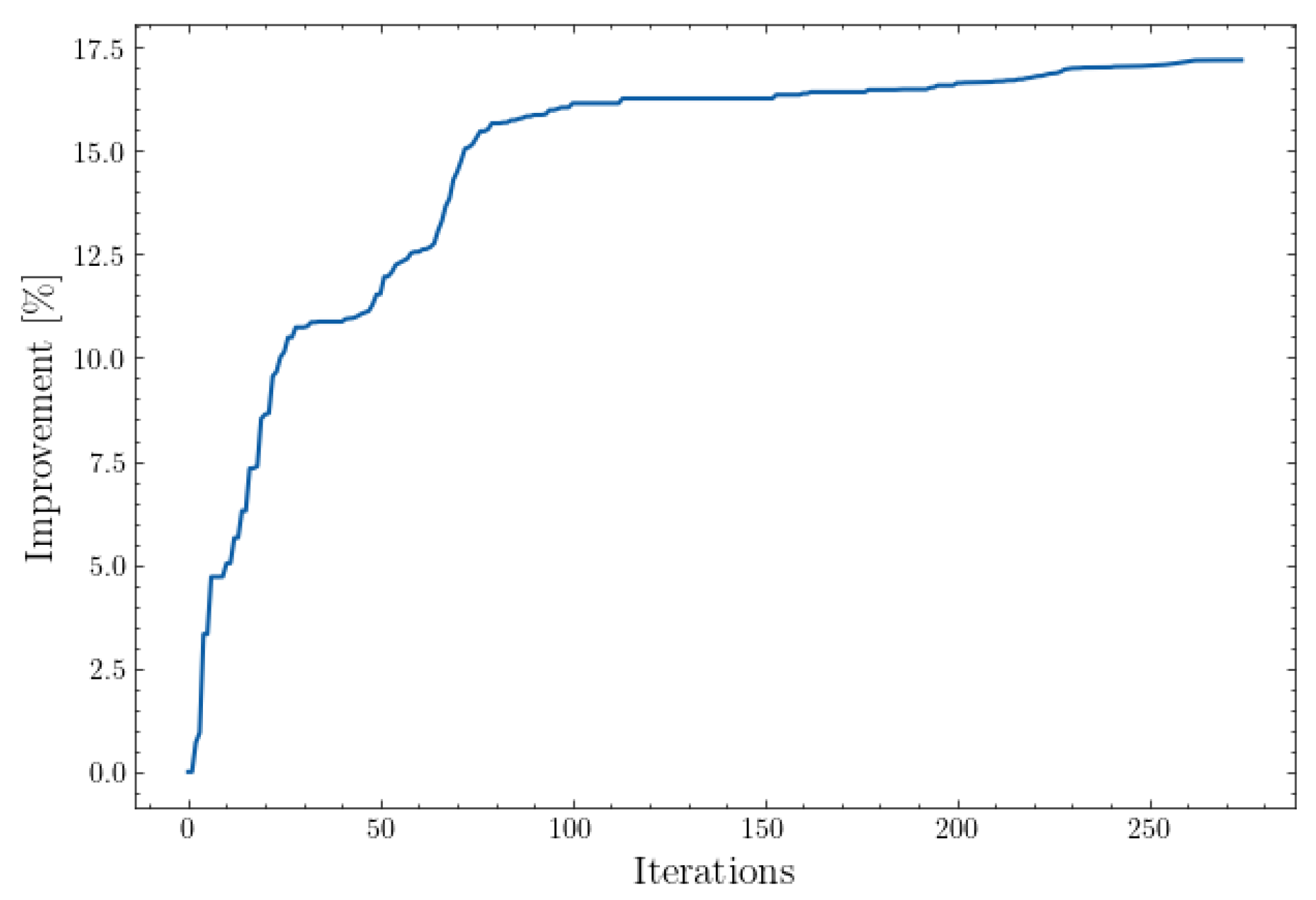
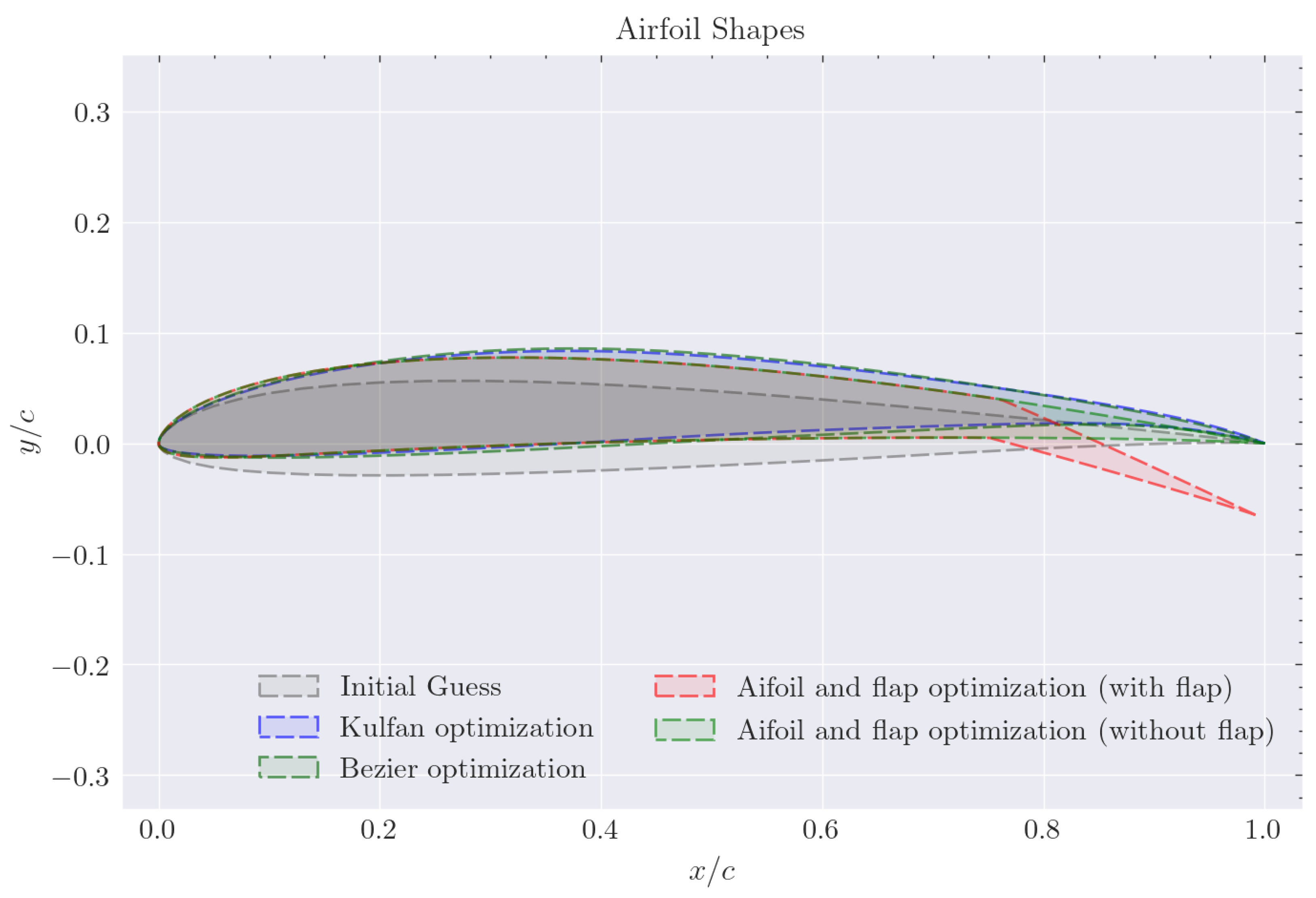
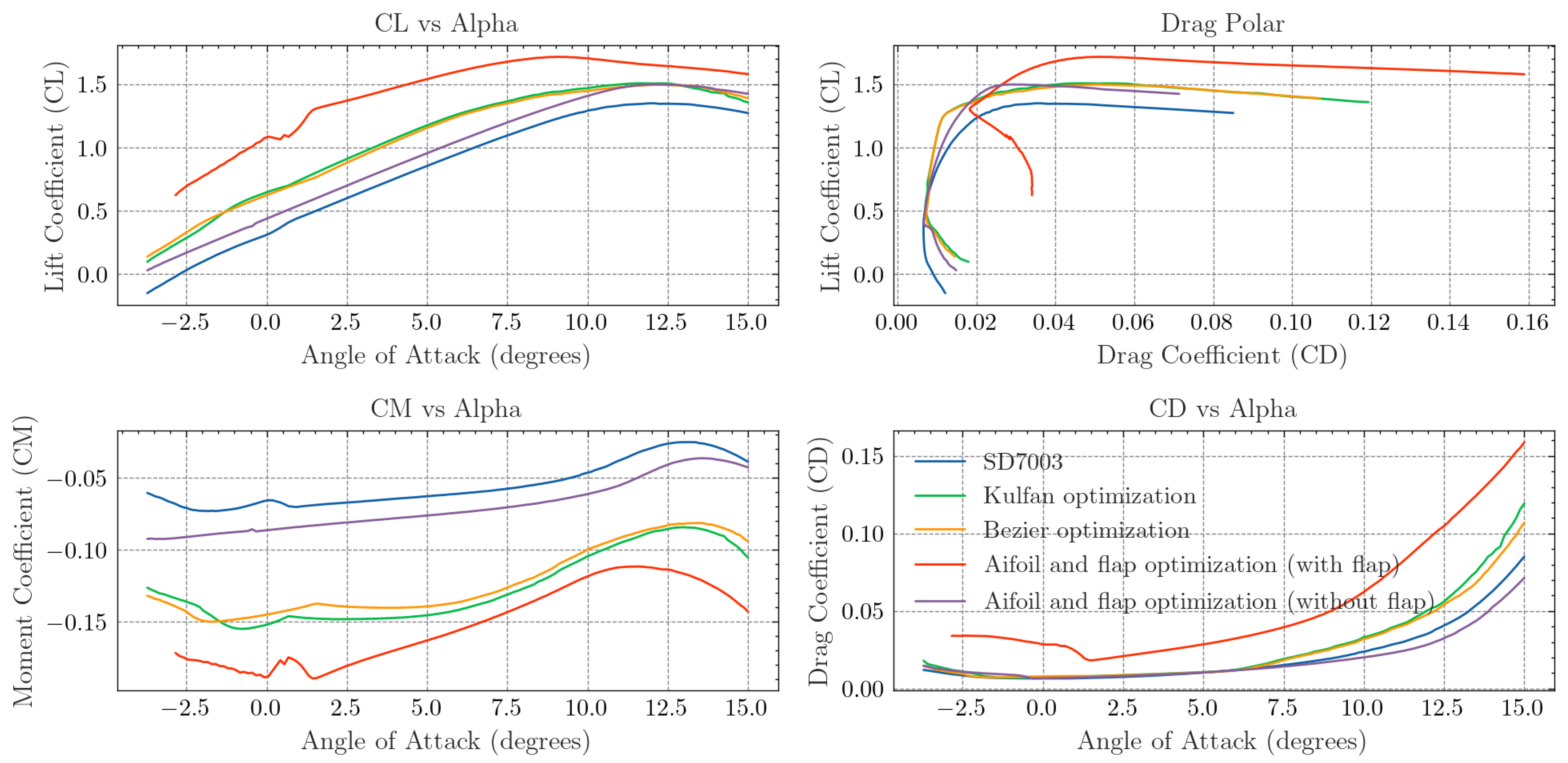
3.1. Optimization
3.2. Global Sensitivity Analysis
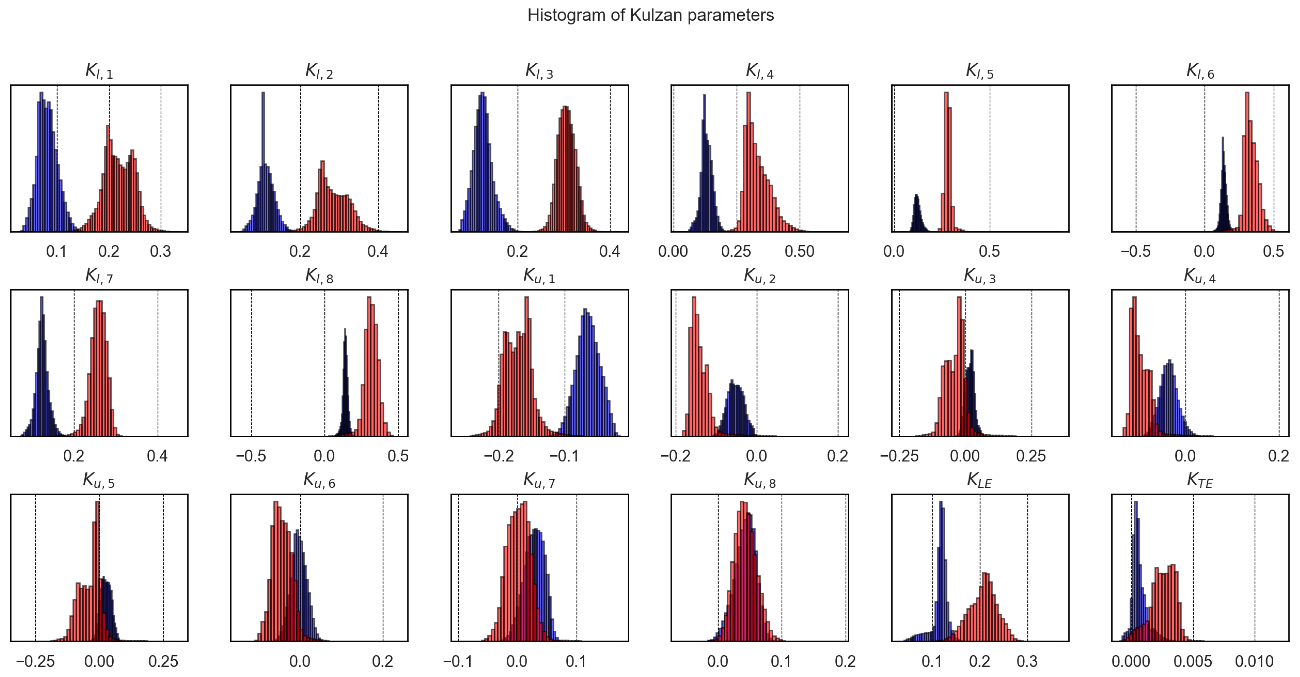
3.3. Generative Design
4. Conclusions
Author Contributions
Funding
Institutional Review Board Statement
Informed Consent Statement
Data Availability Statement
Conflicts of Interest
References
- Hicks, R.; Murman, E.; Vanderplaats, G. An Assessment of Airfoil Design by Numerical Optimization; NASA: Mountain View, CA, USA, 1974. [Google Scholar]
- Hicks, R.M.; Vanderplaats, G.N. Application of Numerical Optimization to the Design of Supercritical Airfoils without Drag-Creep. In Proceedings of the SAE Technical Paper Series, 400 Commonwealth Drive, Warrendale, PA, USA, 3–4 January 1977. [Google Scholar]
- Drela, M. Low-Reynolds-number airfoil design for the M.I.T. Daedalus prototype—A case study. J. Aircr. 1988, 25, 724–732. [Google Scholar] [CrossRef]
- Drela, M. Pros & Cons of Airfoil Optimization. In Frontiers of Computational Fluid Dynamics 1998; World Scientific: Singapore, 1998; pp. 363–381. [Google Scholar]
- Li, W.; Huyse, L.; Padula, S. Robust airfoil optimization to achieve drag reduction over a range of Mach numbers. Struct. Multidiscip. Optim. 2002, 24, 38–50. [Google Scholar] [CrossRef]
- Zingg, D.; Elias, S. On Aerodynamic Optimization Under a Range of Operating Conditions. In Proceedings of the 44th AIAA Aerospace Sciences Meeting and Exhibit, Reno, NV, USA, 9–12 January 2006. [Google Scholar]
- Mirzaei, M.; Nasrin Hosseini, S.; Roshanian, J. Single and multi-point optimization of an airfoil using gradient method. Aircr. Eng. Aerosp. Technol. 2007, 79, 611–620. [Google Scholar] [CrossRef]
- Ulker, F.D.; Doostan, A.; Drela, M. Stochastic Gradient Optimization of Transonic Airfoils. In Proceedings of the AIAA Scitech 2021 Forum, Reston, VA, USA, 11–21 January 2021. [Google Scholar]
- Vicini, A.; Quagliarella, D. Inverse and direct airfoil design using a multiobjective genetic algorithm. AIAA J. 1997, 35, 1499–1505. [Google Scholar] [CrossRef]
- Wang, Y.-Y.; Zhang, B.-Q.; Chen, Y.-C. Robust airfoil optimization based on improved particle swarm optimization method. Appl. Math. Mech. 2011, 32, 1245–1254. [Google Scholar] [CrossRef]
- Wickramasinghe, U.K.; Carrese, R.; Li, X. Designing airfoils using a reference point based evolutionary many-objective particle swarm optimization algorithm. In Proceedings of the IEEE Congress on Evolutionary Computation, Barcelona, Spain, 18–23 July 2010; IEEE: Piscataway, NJ, USA, 2010. [Google Scholar]
- Mirjalili, S.; Dong, J.S.; Lewis, A. Nature-Inspired Optimizers: Theories, Literature Reviews and Applications; Springer: Berlin/Heidelberg, Germany, 2019. [Google Scholar]
- Echeverría, F.; Mallor, F.; San Miguel, U. Global sensitivity analysis of the blade geometry variables on the wind turbine performance. Wind Energy 2017, 20, 1601–1616. [Google Scholar] [CrossRef]
- Mohamed Abubacker Siddique, P.M.; Prince Raj, L. Sensitivity analysis of geometric parameters on the aerodynamic performance of a multi-element airfoil. Aerosp. Sci. Technol. 2023, 132, 108074. [Google Scholar] [CrossRef]
- Storlie, C.B.; Swiler, L.P.; Helton, J.C.; Sallaberry, C.J. Implementation and evaluation of nonparametric regression procedures for sensitivity analysis of computationally demanding models. Reliab. Eng. Syst. Saf. 2009, 94, 1735–1763. [Google Scholar] [CrossRef]
- Ribeiro, A.; Awruch, A.; Gomes, H. An airfoil optimization technique for wind turbines. Appl. Math. Model. 2012, 36, 4898–4907. [Google Scholar] [CrossRef]
- Yilmaz, E.; German, B. A Convolutional Neural Network Approach to Training Predictors for Airfoil Performance. In Proceedings of the 18th AIAA/ISSMO Multidisciplinary Analysis and Optimization Conference, Denver, CO, USA, 5–9 June 2017. [Google Scholar]
- Du, X.; He, P.; Martins, J.R. Rapid airfoil design optimization via neural networks-based parameterization and surrogate modeling. Aerosp. Sci. Technol. 2021, 113, 106701. [Google Scholar] [CrossRef]
- Bouhlel, M.A.; He, S.; Martins, J.R.R.A. Scalable gradient–enhanced artificial neural networks for airfoil shape design in the subsonic and transonic regimes. Struct. Multidiscip. Optim. 2020, 61, 1363–1376. [Google Scholar] [CrossRef]
- Sharpe, P.D. Accelerating Practical Engineering Design Optimization with Computational Graph Transformations. Ph.D. Thesis, Massachusetts Institute of Technology, Cambridge, MA, USA, 2024. [Google Scholar]
- Chen, W.; Chiu, K.; Fuge, M.D. Airfoil Design Parameterization and Optimization Using Bézier Generative Adversarial Networks. AIAA J. 2020, 58, 4723–4735. [Google Scholar] [CrossRef]
- Chen, W.; Chiu, K.; Fuge, M. Aerodynamic Design Optimization and Shape Exploration using Generative Adversarial Networks. In Proceedings of the AIAA Scitech 2019 Forum, San Diego, CA, USA, 7–11 January 2019. [Google Scholar]
- Wang, J.; Li, R.; He, C.; Chen, H.; Cheng, R.; Zhai, C.; Zhang, M. An inverse design method for supercritical airfoil based on conditional generative models. Chin. J. Aeronaut. 2022, 35, 62–74. [Google Scholar] [CrossRef]
- Sun, K.; Wang, W.; Cheng, R.; Liang, Y.; Xie, H.; Wang, J.; Zhang, M. Evolutionary generative design of supercritical airfoils: An automated approach driven by small data. Complex Intell. Syst. 2023, 10, 1167–1183. [Google Scholar] [CrossRef]
- Sekar, V.; Zhang, M.; Shu, C.; Khoo, B.C. Inverse Design of Airfoil Using a Deep Convolutional Neural Network. AIAA J. 2019, 57, 993–1003. [Google Scholar] [CrossRef]
- Achour, G.; Sung, W.J.; Pinon-Fischer, O.J.; Mavris, D.N. Development of a Conditional Generative Adversarial Network for Airfoil Shape Optimization. In Proceedings of the AIAA Scitech 2020 Forum, Orlando, FL, USA, 6–10 January 2020. [Google Scholar]
- Masters, D.A.; Taylor, N.J.; Rendall, T.; Allen, C.B.; Poole, D.J. A geometric comparison of aerofoil shape parameterisation methods. In Proceedings of the 54th AIAA Aerospace Sciences Meeting, San Diego, CA, USA, 4–8 January 2016. [Google Scholar]
- Hicks, R.; Henne, P. Wing design by numerical optimization. In Proceedings of the Aircraft Systems and Technology Meeting, Seattle, WA, USA, 22–24 August 1977. [Google Scholar]
- Rendall, T.C.S.; Allen, C.B. Unified fluid–structure interpolation and mesh motion using radial basis functions. Int. J. Numer. Methods Eng. 2007, 74, 1519–1559. [Google Scholar] [CrossRef]
- Sobieczky, H. Parametric Airfoils and Wings. In Notes on Numerical Fluid Mechanics (NNFM); Vieweg+Teubner Verlag: Wiesbaden, Germany, 1999; pp. 71–87. [Google Scholar]
- Prautzsch, H.; Paluszny, M.; Böhm, W. Métodos de Bézier y B-Splines; KIT Scientific Publishing: Singapore, 2005. [Google Scholar]
- Kulfan, B.; Bussoletti, J. “Fundamental” Parameteric Geometry Representations for Aircraft Component Shapes. In Proceedings of the 11th AIAA/ISSMO Multidisciplinary Analysis and Optimization Conference, Portsmouth, VA, USA, 6–8 September 2006. [Google Scholar]
- Selig, M. UIUC Airfoil Data Site; University of Illinois Urbana-Champaign: Champaign, IL, USA, 2024. [Google Scholar]
- Selvan, K.M. On The Effect Of Shape Parameterization On Aerofoil Shape Optimization. Int. J. Res. Eng. Technol. 2015, 4, 123–133. [Google Scholar] [CrossRef]
- Sripawadkul, V.; Padulo, M.; Guenov, M. A Comparison of Airfoil Shape Parameterization Techniques for Early Design Optimization. In Proceedings of the 13th AIAA/ISSMO Multidisciplinary Analysis Optimization Conference, Fort Worth, TX, USA, 13–15 September 2010. [Google Scholar]
- Song, X.; Wang, L.; Luo, X. Airfoil optimization using a machine learning-based optimization algorithm. J. Phys. Conf. Ser. 2022, 2217, 012009. [Google Scholar] [CrossRef]
- Akram, M.T.; Kim, M.H. Aerodynamic Shape Optimization of NREL S809 Airfoil for Wind Turbine Blades Using Reynolds-Averaged Navier Stokes Model—Part II. Appl. Sci. 2021, 11, 2211. [Google Scholar] [CrossRef]
- Fatchulloh, M.A.; Arini, N.R. Airfoil profile modifications based on Bezier Curve and Optimization using PSO. In Proceedings of the 2024 International Electronics Symposium (IES), Denpasar, Indonesia, 6–8 August 2024; IEEE: Piscataway, NJ, USA, 2024; pp. 100–106. [Google Scholar]
- Ümütlü, H.C.A.; Kiral, Z. Airfoil Shape Optimization Using Bézier Curve And Genetic Algorithm. Aviation 2022, 26, 32–40. [Google Scholar] [CrossRef]
- Selig, M.S. Summary of Low Speed Airfoil Data; Soartech: Ann Arbor, MI, USA, 1995. [Google Scholar]
- Le Gratiet, L.; Marelli, S.; Sudret, B. Metamodel-Based Sensitivity Analysis: Polynomial Chaos Expansions and Gaussian Processes. In Handbook of Uncertainty Quantification; Springer International Publishing: Cham, Switzerland, 2017; pp. 1289–1325. [Google Scholar]
- Saltelli, A. Global sensitivity analysis: An introduction. In Proceedings of the 4th International Conference on Sensitivity Analysis of Model Output (SAMO 2004), Santa Fe, NM, USA, 8–11 March 2004. [Google Scholar]
- Rabitz, H.; Aliş, Ö.F. General foundations of high-dimensional model representations. J. Math. Chem. 1999, 25, 197–233. [Google Scholar] [CrossRef]
- Rabitz, H. Global Sensitivity Analysis for Systems with Independent and/or Correlated Inputs. Procedia-Soc. Behav. Sci. 2010, 2, 7587–7589. [Google Scholar] [CrossRef]
- Kennedy, J.; Eberhart, R. Particle swarm optimization. In Proceedings of the ICNN’95—International Conference on Neural Networks, Perth, WA, Australia, 27 November–1 December 1995; IEEE: Piscataway, NJ, USA, 1995; Volume 4, pp. 1942–1948. [Google Scholar]
- Miranda, L.J.V. PySwarms, a research-toolkit for Particle Swarm Optimization in Python. J. Open Source Softw. 2018, 3, 433. [Google Scholar] [CrossRef]
- Sharpe, P.D. AeroSandbox: A Differentiable Framework for Aircraft Design Optimization. Master’s Thesis, Massachusetts Institute of Technology, Cambridge, MA, USA, 2021. [Google Scholar]
- Wahba, G. Spline Models for Observational Data; Society for Industrial and Applied Mathematics: Philadelphia, PA, USA, 1990. [Google Scholar] [CrossRef]
- Drela, M. XFOIL: An Analysis and Design System for Low Reynolds Number Airfoils; Springer: Berlin/Heidelberg, Germany, 1989; pp. 1–12. [Google Scholar] [CrossRef]
- Coder, J.G.; Maughmer, M.D. Comparisons of Theoretical Methods for Predicting Airfoil Aerodynamic Characteristics. J. Aircr. 2014, 51, 183–191. [Google Scholar] [CrossRef]
- McKay, M.D.; Beckman, R.J.; Conover, W.J. A Comparison of Three Methods for Selecting Values of Input Variables in the Analysis of Output from a Computer Code. Technometrics 1979, 21, 239. [Google Scholar] [CrossRef]
- Derksen, R.; Rogalsky, T. Bezier-PARSEC: An optimized aerofoil parameterization for design. Adv. Eng. Softw. 2010, 41, 923–930. [Google Scholar] [CrossRef]


| Cruise Full Speed | Cruise Lower Speed | Climb | Take off | |
|---|---|---|---|---|
| v | 25 | 20 | 15 | 12.5 |
| Re | 3.42 | 2.74 | 2.05 | 1.71 |
| M | 0.074 | 0.059 | 0.044 | 0.037 |
| 0.427 | 0.667 | 1.186 | 1.708 |
| Kulfan CST [%] | Bézier Curves [%] | |
|---|---|---|
| OP 1 | 2.3 | 0.5 |
| OP 2 | 25.3 | 19.6 |
| OP 3 | 55.6 | 55.5 |
| OP 4 | 5.2 | 5.2 |
| Thickness t | Max. Thickness Location [%] | Camber c | Max. Camber Location [%] | TE Thickness | |
|---|---|---|---|---|---|
| Min. values | 6 | 15 | 0 | 30 | 0 |
| Max. values | 12 | 40 | 4 | 60 | 2 |
| Variable | Sa | Sb | S | ST |
|---|---|---|---|---|
| 0.12 (±0.01) | −0.043 (±0.00) | 0.077 (±0.01) | 0.28 (±0.03) | |
| 0.067 (±0.01) | −0.040 (±0.01) | 0.026 (±0.01) | 0.13 (±0.02) | |
| 0.17 (±0.01) | −0.055 (±0.01) | 0.12 (±0.01) | 0.31 (±0.04) | |
| 1.4 (±0.00) | −2.4 (±0.00) | 1.1 (±0.00) | 0.011 (±0.01) | |
| TE gap | 6.8 (±0.00) | −2.6 (±0.00) | 4.0 (±0.00) | 7.0 (±0.00) |
| / | 0.093 (±0.02) | −0.043 (±0.01) | 0.055 (±0.01) | |
| / | 0.17 (±0.02) | −0.043 (±0.01) | 0.14 (±0.02) | |
| / | 4.4 (±0.00) | 3.1 (±0.00) | 4.7 (±0.00) | |
| /TE gap | 3.3 (±0.00) | −1.1 (±0.00) | 2.1 (±0.00) | |
| / | 0.064 (±0.01) | −0.029 (±0.01) | 0.046 (±0.01) | |
| / | 2.7 (±0.00) | −4.4 (±0.00) | 2.2 (±0.00) | |
| /TE gap | 2.4 (±0.00) | −3.4 (±0.00) | 1.9 (±0.00) | |
| / | 2.2 (±0.00) | −6.7 (±0.00) | 2.1 (±0.00) | |
| /TE gap | 2.7 (±0.00) | −9.8 (±0.00) | 1.7 (±0.00) | |
| /TE gap | 1.5 (±0.00) | −4.9 (±0.00) | 9.1 (±0.00) |
Disclaimer/Publisher’s Note: The statements, opinions and data contained in all publications are solely those of the individual author(s) and contributor(s) and not of MDPI and/or the editor(s). MDPI and/or the editor(s) disclaim responsibility for any injury to people or property resulting from any ideas, methods, instructions or products referred to in the content. |
© 2025 by the authors. Licensee MDPI, Basel, Switzerland. This article is an open access article distributed under the terms and conditions of the Creative Commons Attribution (CC BY) license (https://creativecommons.org/licenses/by/4.0/).
Share and Cite
Rouco, P.; Orgeira-Crespo, P.; Rey González, G.D.; Aguado-Agelet, F. Airfoil Optimization and Analysis Using Global Sensitivity Analysis and Generative Design. Aerospace 2025, 12, 180. https://doi.org/10.3390/aerospace12030180
Rouco P, Orgeira-Crespo P, Rey González GD, Aguado-Agelet F. Airfoil Optimization and Analysis Using Global Sensitivity Analysis and Generative Design. Aerospace. 2025; 12(3):180. https://doi.org/10.3390/aerospace12030180
Chicago/Turabian StyleRouco, Pablo, Pedro Orgeira-Crespo, Guillermo David Rey González, and Fernando Aguado-Agelet. 2025. "Airfoil Optimization and Analysis Using Global Sensitivity Analysis and Generative Design" Aerospace 12, no. 3: 180. https://doi.org/10.3390/aerospace12030180
APA StyleRouco, P., Orgeira-Crespo, P., Rey González, G. D., & Aguado-Agelet, F. (2025). Airfoil Optimization and Analysis Using Global Sensitivity Analysis and Generative Design. Aerospace, 12(3), 180. https://doi.org/10.3390/aerospace12030180