New Method for Improving Tracking Accuracy of Aero-Engine On-Board Model Based on Separability Index and Reverse Searching

Abstract

Throughout its service life, an aero-engine will experience a series of health conditions due to the inevitable performance degradation of its major components, and characteristics will deviate from their initial states. For improving tracking accuracy of the self-tunning on-board engine model on the engine output variables throughout the engine service life, a new method based on the separability index and reverse search algorithm was proposed in this paper. By using this method, a qualified training set of neural networks was created on the basis of eSTORM (enhanced Self Tuning On-board Real-time Model) database, and the problem that the accuracy of neural networks is reduced or even that the training process is not convergent can be solved. Compared with the method of introducing sample memory factors, the method proposed in this paper makes the self-tunning on-board model maintain higher tracking accuracy in the whole engine life, and the algorithm is simple enough for implementation. Finally, the training set center generated in the calculation process of the proposed method could be used for the real-time monitoring of the engine gas path parameters without additional calculations. Compared with the commonly used sliding window method, the proposed method avoids the problem of low algorithm efficiency caused by fewer abnormal data samples.

1. Introduction

Modern aero-engine is a complex aero-dynamic, thermal, and mechanical equipment with a harsh working environment and strong nonlinear characteristics. In order to ensure the safe and reliable operation of the engine under all operating conditions, while realizing its full performance potential, engine control systems have evolved over the past few decades and are able to diagnose faults and determine the health state of the engine online [1,2]. Advanced control and fault diagnosis systems need to obtain all kinds of state information of engine accurately in real time. However, due to many reasons such as space, structure, and material, the parameters that can be measured directly by sensors are very limited. In order to solve this contradiction, on-board engine model technology has been put forward, and has been paid attention to by many scholars and engineers in the past decades.

There are many challenges that need to be overcome in order to track the engine state accurately in real time. Aero-engine is a strong nonlinear aero-dynamic, thermal, and mechanical equipment with a wide operating envelope. Across the whole operating envelope, the engine characteristics will change significantly. Throughout the life of the engine, due to blade corrosion, erosion, wear, combustion characteristics change, and other reasons, engine components will slowly decline, and the overall characteristics of the engine gradually deviate from its initial state. The change in the power and air flow extracted from the engine will cause the engine behavior to deviate from the preset state. Meanwhile, engine characteristics could suddenly be changed due to faults, FOD (Foreign Object Damage), and other unexpected events. Last but not least, the cleaning of engine components during service, planned maintenance, and component replacement can partially restore engine performance [3]. An aero-engine on-board model can usually only represent a nominal state of a certain type of engine, as it is difficult for the model to accurately reflect all changes caused by the factors mentioned above.

In order to improve the tracking accuracy of an aero-engine on-board model, a lot of research work was conducted. In 1989, R. H. Luppold [4] proposed STORM (Self Tuning On-board Real-time Model), which used a linear model and Kalman filter to estimate the performance parameters of engine components, so that the on-board model could track the performance changes in engine components and improve the model accuracy. From 2003 to 2008, Brotherton and Volponi et al. [5,6,7,8,9] proposed that based on the self-tunning on-board model, the output parameters of the piecewise linear model were modified by neural networks, that is eSTORM (enhanced Self Tuning On-board Real-time Model). The training set of the neural networks was generated by a real-time Gaussian clustering algorithm. Finally, eSTORM was verified on the PW6000 commercial engine (Pratt & Whitney, East Hartford, CT, USA). eSTORM introduces the data-driven modeling method on the basis of the model, which is based on the physical mechanism. Many scholars continue to improve the on-board model along this technical route. Lu et al. [10] from Nanjing University of Aeronautics and Astronautics adopted an LPV (Linear Parameter Varying) model instead of a PL (piecewise linear) model; at the same time, Lu replaced a neural network with IR-KELM (Independent Reduction Kernel Extreme Learning Machine). IR-KELM divides the engine real-time data samples into training set B and constraint set P. The training set is used to train the neural network directly, and the constraint set is used to modify the network. Li et al. [11] adopted a neural network to predict the steady-state part of the on-board engine model. The training data of the neural network comes from the component level nonlinear engine model simulation. Meanwhile, the similarity criterion is used to compress the training set, which improves the training speed. Zheng Qiangang [12] used the MGD (Mini-batch Gradient Descent) method to train neural networks, which improves the training efficiency; meanwhile, they added a penalty item, which is the sum of weights in each layer, to the objective function to prevent overfitting in training. Zheng [13,14] also used deep neural networks to fit the nonlinear characteristics of an aero-engine for improving the model tracking accuracy. Zhao et al. [15] designed the thrust estimator with particle swarm core extreme learning machine, which improved the accuracy and speed of thrust estimation. Xiang et al. [16] adopted the fusion method of neural network and propulsion system matrix to build a self-tunning on-board model, which improves the average accuracy of the model under large operating envelope and multiple states.

In recent years, with the development of data technology, the engine model using only data-driven technology has attracted the attention of many scholars. S. Sina Tayarani-Bathaie et al. from Concordia University added IIR (Infinite Impulse Response) filter to the neuron of the neural network to form a dynamic neuron and then formed a dynamic neural network to simulate the dynamics of a turbo-engine [17]. Manuel Arias Chao et al. used a CNN to simulate engine dynamics to speed up the calculation process [18]. Serhii Vladov et al. from Kharkiv National University used a neural network with dynamic stack memory to simulate multiple working modes of a turboshaft engine [19]. M Shuai et al. from Northwestern Polytechnical University compared the performance of LSTM, GRU, and other dynamic networks for engine modeling, and concluded that GRU is superior to other dynamic networks in training and prediction [20].

In the above research work, the differences between the data samples produced by an aero-engine in different health states were not discussed in detail. In fact, an engine that has experienced component performance degradation will consume more fuel, produce higher turbine exhaust temperature, and exhibit higher unit fuel consumption than a brand new engine to achieve the same control objectives (such as low pressure rotor speed) under the same engine control system. These characteristic differences, through real-time sampling, will produce different data sets. If these data sets are used indiscriminately to train the on-board neural networks, no matter whether these neural networks are used for output compensation or for representing component characteristics, “confusion” will be introduced, resulting in accuracy reduction and even non-convergence of the training process.

This paper presents an algorithm for generating a qualified training set for neural networks based on the separability index and reverse searching of database elements to improve the accuracy of neural networks and training process. The algorithm searches and adds the database elements to a subset in reverse order of database (for example, the GMM database), and calculates the separability index of the data subset. When the separability index exceeds the preset threshold value, the search stops, and the final data subset is used as the training set of the neural networks. This algorithm eliminates the elements in the database that no longer represent the current health state of the engine, improves the training accuracy of the neural networks, and also increases the training speed by reducing the training samples.

The major structure of this paper is as follows: Section 1 presents the introduction. Section 2 introduces the eSTORM model architecture and the algorithms of each sub-module. Section 3 simulates the engine component degradation process and analyzes the reasons for the accuracy reduction in neural network compensation. In Section 4, the separability index and reverse searching algorithm are introduced. Section 5 represents the effect of the proposed method through simulation. Section 6 discusses the possible application of the separability index and reverse searching algorithm in engine gas path monitoring, and Section 7 is the conclusion.

2. eSTORM and GMM

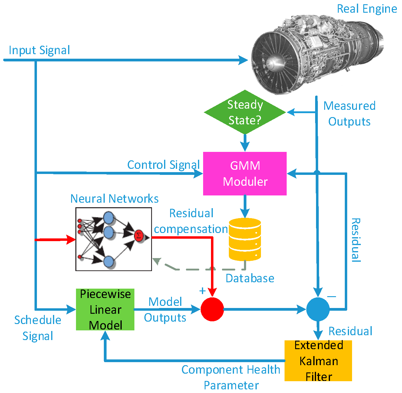
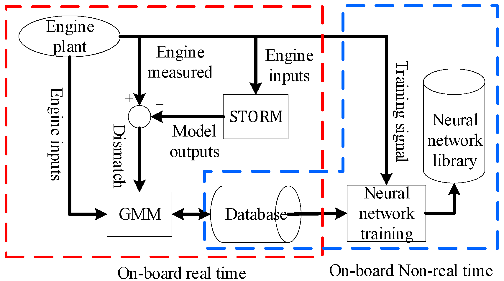
2.1. eSTORM Structure

The eSTORM structure, proposed by Volponi et al. on the basis of the STORM structure, includes a piecewise linear model, extended Kalman filter, GMM (Gaussian Mixture Model) module, which includes a real-time clustering algorithm and database, and neural network units. The eSTORM structure is represented in Figure 1.

In Figure 1, the piecewise linear model represents the behavior of the engine near the steady-state operating point. The piecewise linear model is scheduled in an entire engine operating envelope, and the scheduling parameters usually include environmental parameters (altitude, Mach number) and engine state parameters (low pressure rotor speed, nozzle throat area, etc.). The residuals between the piecewise linear model outputs and the engine sensor outputs are sent to the Kalman filter, which estimates the engine state and health parameters. The component health parameters are fed back to the piecewise linear model for increasing model accuracy.

Due to underdetermined estimation, unmodeled dynamics, different engine operating conditions, etc., there are still inevitable output residuals between the modified piecewise linear model and the real engine. These residuals and engine control inputs are sent to the GMM module to form a database by Gaussian clustering calculation. The elements in this database represent the degree of mismatch between the on-board model and the real engine under different environment and operating conditions. At the end of each flight cycle, the neural networks are trained using the newly formed database. A flight cycle usually consists of starting up, taking off, climbing, cruising, descending, and landing. Accordingly, the engine will experience several segments such as ground idle, maximum, cruise, and flight idle. The trained neural networks can be used to compensate the outputs of the on-board model in all segments according to the current engine environment. Thus, the tracking accuracy is improved and the individual adaptability of the model is increased. The working process of eSTORM is represented in Figure 2.

In Figure 2, engine input variables (wfm, A8, etc.) and residuals between engine outputs and engine model outputs are sent to the GMM module. In this paper, the engine outputs include eight parameters: N1, N2, Tt25, Tt3, Tt6, Pt25, Pt3, and Pt6. The collected data are calculated through clustering to form a database. Therefore, each sample in the database contains the control variables of the engine in a certain working condition and all the output parameter residuals. This part of the work is carried out on-board in real time. At the end of the mission (i.e., after the vehicle has landed), the neural networks are trained based on the newly generated database and saved as a neural network library. In the training process, the samples in the database are taken out as the training set, and the weights and bias values of each layer are corrected until the training accuracy requirements are achieved. After the networks are trained correctly, the weights and bias values will be stored in the neural network library. This part of the work is carried out on-board but in non-real time.

2.2. GMM Module and Algorithm

The GMM module collects the control inputs and output differences between the on-board model and the real engine in real time and determines whether there are elements with similar characteristics in the database. If there is not any data element that represents the current engine characteristics, the GMM module starts a new clustering process and adds a new data element to the database.

The GMM module uses the Mahalanobis distance (MD) to represent the “similarity” of the sampled data at the current time and the database elements. MD is often used for boundary detection and clustering process [21]. For data set $X=\left\{x_1,x_2,\dots ,x_n\right\}$, the general definition of MD is presented in Equation (1).

$$d_{Mi}=\sqrt{{\left(x_i-\overline{x}\right)}^T{C}^{-1}\left(x_i-\overline{x}\right)}$$

(1)

where $d_{Mi}$ indicates the MD between the i-th element and the mean of the data set; $\overline{x}$ denotes the mean of the data set; and $C$ denotes the variance–covariance matrix of the data set. The mathematical expression is as follows:

$$C=diag\left({\sigma }_1^2,{\sigma }_2^2,\dots ,{\sigma }_n^2\right)$$

(2)

In Equation (2), the covariances between the data elements are ignored.

The formulation of MD in this paper is shown in Equation (3).

$$d_M\left(u,D\right)=\sqrt{{\displaystyle \sum _{i=1}^N{\left(\frac{u\left(i\right)-\overline{D}\left(i\right)}{w\left(i\right){\sigma }_D\left(i\right)}\right)}^2}}$$

(3)

where $d_M$ indicates the Mahalanobis distance; $u$ denotes the sample data at the current time, including control inputs and discrepancies between model and engine outputs; $D$ denotes the elements that are already in the database; $N$ indicates the length of data vector; $\overline{D}$ denotes the mean value of $D$ while ${\sigma }_D$ is the standard deviation; and $w\left(i\right)$ refers to the noise sensitive factor of the $i$-th data element, which is used for adjusting the order of magnitude of MD. GMM calculates the MD between the sampled data at the current time and all database elements, and if the smallest distance is still greater than the preset threshold, a new clustering process is launched. The clustering program calculates the mean and standard deviation of the control inputs and output residuals in a certain operating period to construct a new element. In this paper, the GMM module only processes the data of steady-state, so before calculating the Mahalanobis distance, it is necessary to determine whether the engine is in a steady-state condition. The flow chart of the Gaussian clustering algorithm is shown in Figure 3.

In Figure 3, the GMM module uses a real-time algorithm to update the mean and standard deviation of the sampled data. The calculation formula of the mean and standard deviation is shown in Equation (4).

$$\begin{array}{l}{\overline{u}}_N(i)=\left({\displaystyle \frac{N-1}{N}}\right){\overline{u}}_{N-1}(i)+\left({\displaystyle \frac{1}{N}}\right)u_N(i)\\ {\sigma }_N^{(u)}(i)=\sqrt{\left({\displaystyle \frac{N-2}{N-1}}\right){\left[{\sigma }_{N-1}^{(u)}(i)\right]}^2+{\displaystyle \frac{1}{N}}{\left(u_N(i)-{\overline{u}}_{N-1}(i)\right)}^2}\\ \forall i=1,2,...,m_u\end{array}$$

(4)

where ${\overline{u}}_N(i)$ denotes the mean value of clustering process at the current time step, and ${\overline{u}}_{N-1}(i)$ denotes the value at previous time step; ${\sigma }_N^{(u)}(i)$ denotes the standard deviation at the current time step, and ${\sigma }_{N-1}^{(u)}(i)$ denotes the value at previous time step; $N$ denotes the number of samples; $i$ indicates the index of element in data vector; and $m_u$ indicates the number of vector elements.

More detailed descriptions of the Gaussian clustering algorithm can be found in the literature of Volponi [8] and Sun [22].

2.3. Neural Networks and Training Algorithm

The neural networks in eSTORM are used to compensate the discrepancies between outputs of the model and the real engine under different engine operating conditions. Only steady-state conditions are considered, so the perceptron structure involving one hidden layer is adopted in this paper. The number of hidden layer nodes can be adjusted according to the application situation. For avoiding the coupling effect between parameters, every neural network has just one single output node, and each network only compensates one output parameter. The activation function is a symmetric Sigmoid function and is shown in Equation (5).

$$f\left(x\right)={\displaystyle \frac{1-e^{-x}}{1+e^{-x}}}$$

(5)

The cost function of neural network training is the mean squared error function as follows:

$$E={\displaystyle \frac{1}{2N}}{\displaystyle \sum _{i=1}^N{\left(t_i-z_i\right)}^2}$$

(6)

where $E$ refers to the cost function; $t$ indicates the output value of the samples; $z$ indicates the actual output value in the forward calculation; $N$ denotes the number of samples; and $i$ denotes the sample index. In this paper, a Back Propagation training algorithm with a momentum item is adopted, as shown in Equation (7).

$$w_{i+1}=w_i-{\alpha }_i{\displaystyle \frac{\partial E}{\partial w}}+{\beta }_i\left(w_i-w_{i-1}\right)$$

(7)

where $w$ denotes the weight to be corrected, $i$ denotes iteration number, $\partial E/\partial w$ denotes weight correction item; $\alpha$ denotes the learning rate; $w_i-w_{i-1}$ indicates the momentum item; and $\beta$ indicates the coefficient of the momentum item. $\alpha ,\beta \in \left(0, 1\right]$.

3. Problem

The total life of an aero-engine can usually reach thousands of hours, and civil engines can reach up to 20,000 to 30,000 h. In the long service life of the engine, with the increase in service time and number of flight cycles, the overall performance of the engine will degrade due to corrosion and erosion of the rotor blades, changes in the working efficiency of the combustion chamber, wear of the bearing components, and the decline in the efficiency of the heat exchange components.

It can be seen that the database generated by the Gaussian clustering algorithm will store all data samples of the engine from the initial service state to the current state, and these data represent the characteristics of the engine in different health states. As engine service time increases, the components continue to degrade, and the number of elements in the database grow gradually. For example, with the degradation of the high pressure rotor, the engine can still reach the preset rotor speed under the regulation of the control system, but it will produce lower Pt3, higher Tt6 and SFC, and smaller thrust. As the pressure/temperature signal at each engine cross-section changes, the Mahalanobis distance between the sampled data and the existing elements in the database increases gradually. When this distance exceeds the preset threshold, a new clustering process is launched and a new element is generated.

3.1. Illustration of Simulation Model

For illustration, the engine control system and self-tunning on-board model were designed in the Simulink environment, and the performance degradation process of the fan, compressor, high pressure turbine, and low pressure turbine was simulated. The diagram of the engine and control system is shown in Figure 4.

In Figure 4, the real engine is a component level nonlinear model that can accurately reflect the operation of the real engine in full operating envelope. In the simulation model, control noise is added to the control inputs. The diagram of the engine structure and cross-section definition is shown in Figure 5.

A low bypass two-rotor turbofan engine with afterburner is presented in Figure 5. The control variable of the engine is the main fuel flow (wfm), the environmental parameters are altitude (Alt) and Mach number (Ma), and the measurable output variables are N1, N2, Tt25, Tt3, Tt6, Pt25, Pt3, and Pt6, respectively. In addition, the component level model has the inputs of component health parameters, which can adjust the level of component degradation. The model contains eight component health parameters, which are listed in

Table 1. Engine health parameters.

Nomenclature	Parameter	Value Range
FanEffDe	Fan efficiency degradation factor	0~3%
FanWaDe	Fan mass flow degradation factor	0~3%
ComEffDe	High pressure compressor efficiency degradation factor	0~3%
ComWaDe	High pressure compressor mass flow degradation factor	0~3%
HPTEffDe	High pressure turbine efficiency degradation factor	0~3%
HPTWaDe	High pressure compressor mass flow degradation factor	0~3%
LPTEffDe	Low pressure turbine efficiency degradation factor	0~3%
LPTWaDe	Low pressure turbine mass flow degradation factor	0~3%

.

In Table 1, all the health parameters range from 0 to 3%, where 0 indicates that the component is not degraded at all, and a larger value indicates that the engine component is degraded more seriously. The value of more than 3% is not practical because the remaining useful life of the components in this state has almost been exhausted [23].

The piecewise linear model in Figure 4 is obtained by linearizing the component level nonlinear model near its steady-state operating point. When the engine is transitioning from one operating condition to another, the linear model will schedule within the operating envelope according to the environmental conditions and operating states. The extended Kalman filter is obtained from the linear model parameters. It should be noted that due to the limitations of the engine structure and space, the number of sensors installed on the engine is usually less than the health parameters that need to be estimated, which will introduce the problem of underdetermined estimation. In the model presented in this paper, the temperature and pressure sensors are set at the 25, 3, and 6 cross-sections of the engine, and there are a total of six measurable parameters, so for the eight component health parameters, the Kalman filter only estimates six of them, which are efficiency and the mass flow decay factor of the fan, compressor, and low pressure turbine. Detailed illustrations for generating the engine linear model and solving Kalman filters can be found in the literature of Lu [24,25]. The controller in Figure 4 is a classic PID controller, in which the controlled variable is the engine low pressure rotor speed (N1), and the control output is the main fuel mass flow (wfm).

3.2. Simulation Settings and Results

The simulation settings are as follows: the altitude is 4 km, the Mach number is 0.8, and the engine accelerates from 70% to 100% of N1 under the control system. The simulation is carried out repeatedly under the above conditions, and in the process, the degradation level of each engine component is gradually increased, and the change in engine output variables are observed. However, the performance degradation of the aero-engine components in the long-period is affected by many factors, such as the manufacturing of the technology components, fabrication of the engine, operating environment, and maintenance level. It is very difficult to accurately reconstruct the performance degradation trend of the main components of the engine in the simulation environment. According to G. P. Sallee [26], the performance degradation process of the engine components is generally linear with the number of engine working cycles. In this paper, the health parameters of each component are set to increase linearly with the simulation cycles, increasing by 0.1% for each cycle until the health parameters degrade by 3%.

The operation process of the engine during one simulation cycle is shown in Figure 6. The residuals between the outputs of self-tunning on-board model and the component level nonlinear model under different degradation conditions are shown in Figure 7. All parameters in Figure 6 and Figure 7 are normalized with reference to the values of the maximum state of the engine on the ground, and all parameters in the figures are percentages.

As can be seen from Figure 6 and Figure 7, as the degradation of engine model component performance evolves, the output residuals between the piecewise linear model and the nonlinear model will gradually increase, which is caused by underdetermined estimation, reducing the tracking accuracy of the model. It should also be noted that since the simulation was carried out under closed-loop conditions, the accuracy of the controlled variable N1 is guaranteed by the PID controller, so it is less affected by the performance degradation of the engine components.

According to the on-board real-time clustering algorithm described in Section 2.2, all of the historical data will become the element of the GMM database if their MD from each other exceeds the preset threshold. On an engine that has been in service for a long time, when all the elements of the database are used to train the neural networks, those elements generated earlier, which can no longer represent the current characteristics of the engine, will interfere with the training process, reduce the compensation accuracy of the neural networks, or even make the training process non-convergent in severe cases.

4. Separability Index and Algorithm

In order to mitigate the influence of historical data on the training process and improve the tracking accuracy of neural networks, Xu proposed a method to introduce memory factors into training samples. Letting $\lambda$ be the memory factor, $\lambda \in \left(0,1\right)$, then the samples are formulated as follows:

$${\lambda }^n{H}_n, n=0,1,2,\dots$$

(8)

where $H_n$ denotes the samples of a certain time batch, and $n$ denotes the batch index. As can be seen from Equation (7), the earlier the sample is formed in the database, the larger $n$ is, so the smaller its memory factor is [27]. This method reduces the influence of historical data on the training process of neural networks but does not clearly define the batch of samples. If the gradual degradation and sudden changes due to faults are both taken into account, $\lambda$ needs to be optimized.

In this paper, referring to the literature of David L. Davies [28] and James C. Bezdek [29], a method was proposed to improve the quality of training sets of neural networks based on the separability index and reverse search algorithm. The mathematical definition of separability index is as follows:

Let $X=\left\{x_1,x_2,\dots ,x_n\right\}\subset {\Re }^{\mathrm{p}}$ be a set of n feature vectors in p-space, then the separability index of $X$ is defined as follows:

$$S={\displaystyle \frac{1}{n}}{\displaystyle \sum _{i=1}^n{\displaystyle \sum _{j=1}^p{\left(x_{ij}-\overline{V_j}\right)}^q}}, i=1,2,\dots ,n, j=1,2,\dots ,\mathrm{p}$$

(9)

where $S$ denotes the separability index, $n$ denotes number of elements in the data set, and $x$ denotes element of the data set. The subscript $i$ indicates the index of the element in the data set, while $j$ indicates the index of the component in the element. $q$ can be selected according to the situation. If $q=1$, then $S$ represents the average Euclidean Distance; if $q=2$, then $S$ represents the mean square error. In this paper, $q=2$ is adopted. $\overline{V}$ in Equation (9) denotes the center of the data set $X$, and its definition is as follows:

$$\overline{V}={\displaystyle \frac{1}{n}}{\displaystyle \sum _{i=1}^n{x}_i}$$

(10)

The separability index S is the mean square error between all elements in a data set and its center and can be used to represent how dispersed the elements of a data set are. The more dispersed the data set elements are, the larger S is.

The GMM module determines whether new data elements need to be generated in each flight cycle of the engine, and all database elements are arranged in the order of generation time. Since the data elements are obtained under multiple steady-state conditions, it is necessary to classify the data according to the engine operating conditions first, and then the algorithm searches in reverse order in each class to ensure that newer elements can be added to the training set. Finally, the separability index of each class of data is calculated, respectively, and the qualified data in all classes are added to the training set. The algorithm flow chart for generating a qualified training set of neural networks is shown in Figure 8.

By introducing the separability index, S, and reverse searching, the original workflow of the eSTORM model is changed, and the new workflow of eSTORM is shown in Figure 9.

In Figure 9, the elements in the GMM database were first processed by the reverse searching algorithm, then S was calculated. And the qualified training set of the neural networks was generated according to the preset S threshold value. These calculations were carried out on-board in real time. This qualified training set would be used to train the neural networks at the end of every flight cycle. The rest of Figure 9 is the same as Figure 2.

A qualified training set generated under 100% engine operating conditions is shown in Figure 10.

In Figure 10, the blue circles represent the qualified training sample obtained according to the separability index, the green circle represents the center of the qualified training set, and the red asterisk represents the training sample judged as unqualified by the separability index. In Figure 10, the X-axis is the main fuel flow, and the Y-axis is the Tt3 output residual. All data in the figure were normalized.

The method of using the separability index and reverse search algorithm to generate a qualified training set of neural networks has the following advantages:

(1)

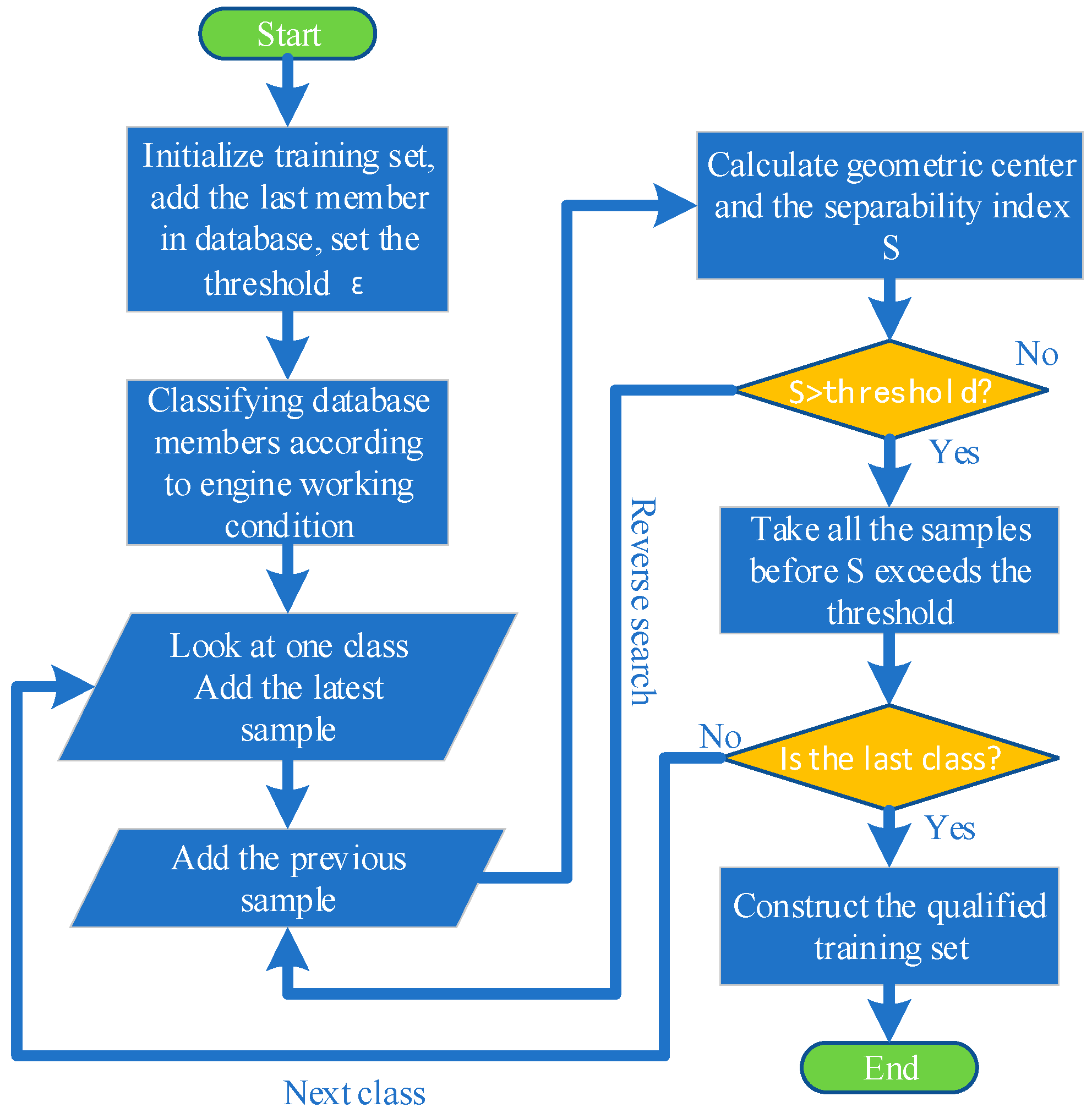
This method can completely eliminate the samples formed earlier in the database that can no longer represent the current state of the engine, improves the tracking accuracy of the neural network, and ensures that the training process always converges.

(2)

By comparing the definition of the separability index in Equation (9) with the cost function of the neural network in Equation (6), it can be found that they are very similar in mathematical form, so the threshold of the separability index can be set according to the cost function of the neural network.

(3)

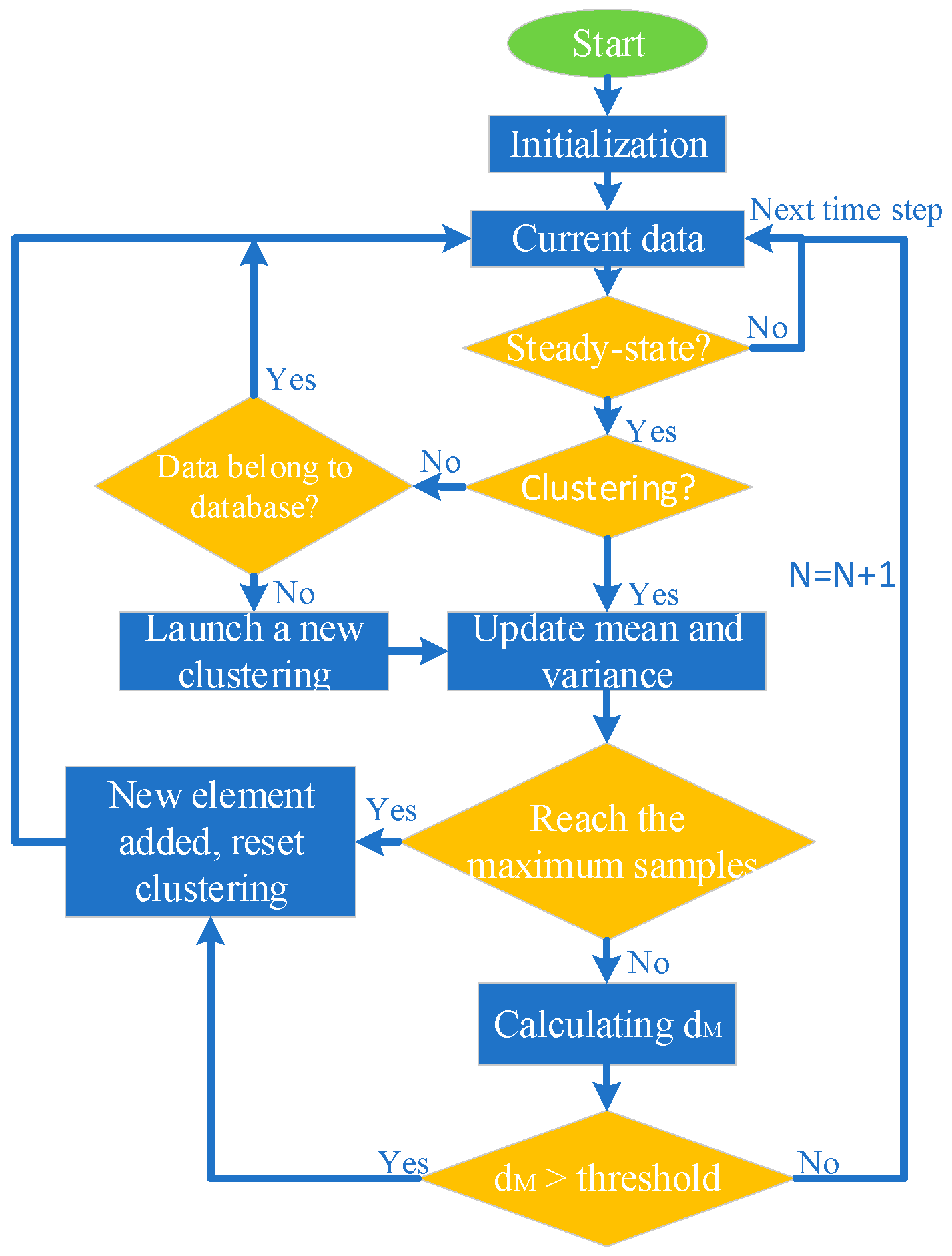
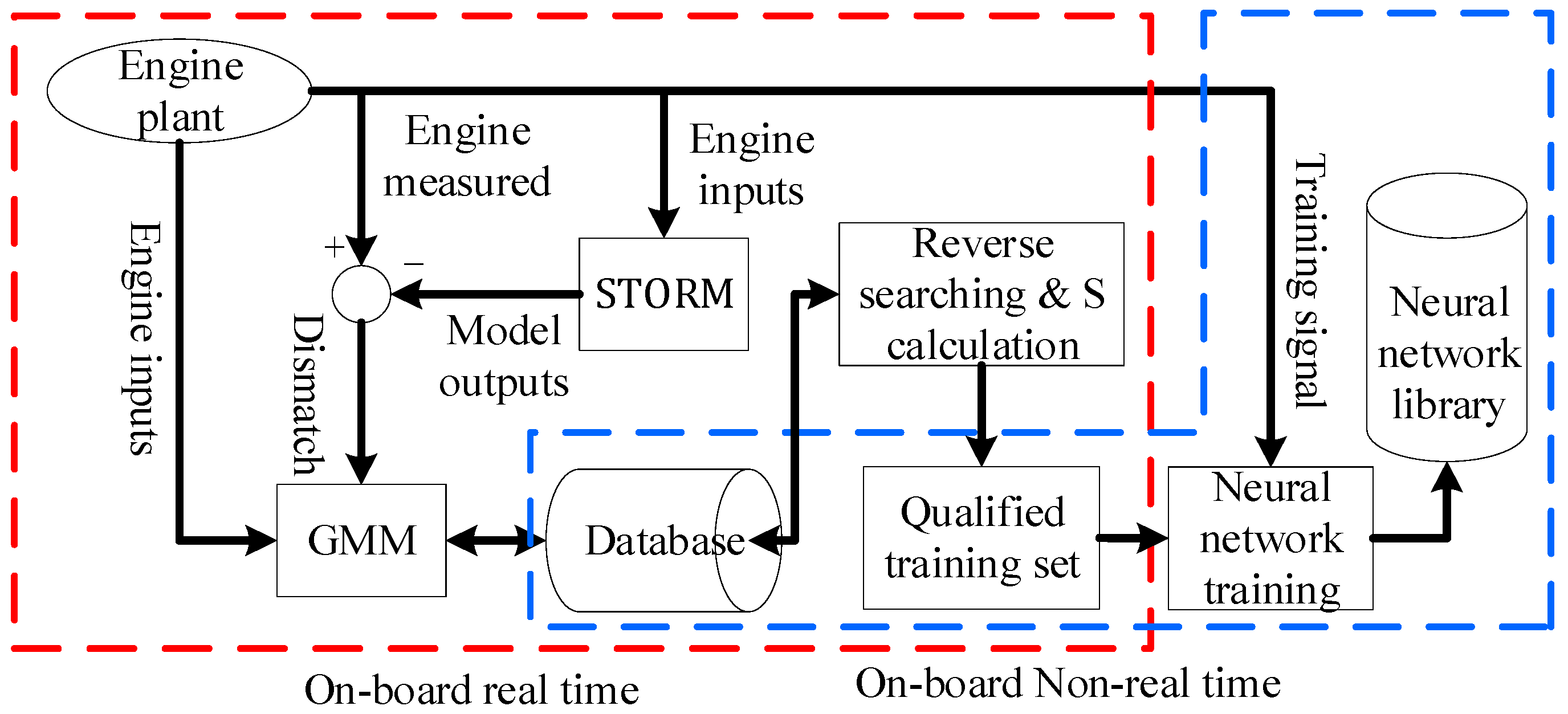
The algorithm is relatively simple for implementation. As shown in Figure 9, the algorithm can run in the on-board environment in real time.

(4)

Finally, because the qualified training set is a subset of the database, which was generated by GMM module, the number of training samples is reduced, and the training speed of the neural network is improved.

5. Simulation and Comparison

In this section, under the same simulation settings as in Section 3.2, eSTORM using memory factor $\lambda$ and separability index S is simulated, respectively, and the tracking accuracy of both is compared in the end. In order to ensure that the neural networks trained by the two methods have a good compensation accuracy, the memory factor is set to 0.6 (training non-convergence may occur above 0.6), and the threshold value of the separability index is set to 10⁻⁶ order of magnitude, which is higher than the accuracy of the cost function of the neural network. The network and the training algorithm are the same as described in Section 2.3, and the training results show that the precision of the cost function reached the level of 10⁻⁵. The comparison of the Tt3 variable obtained by simulation is shown in Figure 11.

In Figure 11, (1) is the working process of the engine model without degradation. As can be seen from the figure, at this time, since there are only data elements representing a brand new engine in the database, the eSTORM model using memory factor $\lambda$ and separability index S can both track the engine output variables accurately. (2) refers to the working process of the engine under 3% degradation condition. (3) and (4) show the tracking errors of eSTORM using the two methods under different degradation conditions, respectively. As can be seen from the figure, as the engine degradation evolves, the tracking accuracy of eSTORM using memory factor $\lambda$ decreases, while that using the separability index $S$ remains high under different health conditions. The comparison of the tracking errors of all output variables under 100% operation condition is listed in

Table 2. Comparison of tracking discrepancy of engine parameters.

Parameters	Degradation	Tracking Error (%)
		STORM	eSTORM with $\mathit{\lambda }$	eSTORM with $\mathit{S}$
N2	1%	1.659	0.414	0.387
	2%	2.103	1.244	0.059
	3%	2.622	1.844	0.316
Tt25	1%	1.191	0.823	0.237
	2%	1.583	0.979	0.235
	3%	1.975	1.027	0.237
Tt3	1%	2.197	0.930	0.309
	2%	3.933	1.228	0.277
	3%	5.510	1.344	0.195
Tt6	1%	1.034	0.884	0.291
	2%	1.676	0.924	0.239
	3%	2.432	0.986	0.272
Pt25	1%	0.993	0.967	0.433
	2%	1.507	1.059	0.382
	3%	2.042	0.978	0.232
Pt3	1%	0.937	0.743	0.311
	2%	1.371	0.740	0.245
	3%	1.616	0.737	0.252
Pt6	1%	0.922	0.820	0.264
	2%	1.345	0.804	0.340
	3%	1.768	0.883	0.242

.

As can be seen from Table 2, in general, the eSTORM with memory factors $\lambda$ can ensure the convergence of the training process of the neural networks, thus improving the tracking accuracy of the model, but it is still affected by the early database elements. It can also be seen that the model with separability index S not only guarantees the training convergence of neural networks but also has high tracking accuracy because it is not affected by early elements. Finally, it should be noted that since the self-tunning on-board model works under control in a closed-loop system, the accuracy of the controlled variable N1 is guaranteed by the PID controller, so it is not listed in Table 2.

6. Discussion of Separability Index in Engine Gas Path Monitoring

The separability index S can be used not only to generate qualified training set, but also to monitor engine gas path parameters.

Each component of the center $\overline{V}$, which is calculated from Equation (10), represents the short-term average of the residual of a temperature or pressure variable over a period of time. By looking at all of this series of short-term averages, it is possible to obtain the tendency of engine output variables to deviate from their nominal state. The data center evolution trends of Tt3 and Tt6 residuals are shown in Figure 12.

In Figure 12, the amplitude and trend of an output variable deviating from its nominal value can be observed directly, and then the decision can be made whether there is an anomaly or fault. If a sensor drift fault occurs, a sudden change point will be produced in the corresponding tendency chart.

Compared with the traditional sliding window method for gas path monitoring [30,31], the method of using separability index and reverse searching in database has the following advantages:

(1)

After the Gaussian clustering process of eSTORM, the original gas path parameters of the engine have formed a database containing all steady-state operating points, and the influence of noise in the system and measurement are mitigated. The data set constructed by using the separability index and reverse searching represents the current state of the engine. Therefore, the monitoring of the parameter trends does not require additional calculations.

(2)

Because the data samples are compressed in time dimension, there is no problem of low algorithm efficiency caused by too few abnormal samples in the sliding window method.

7. Conclusions

In this paper, aiming at the influence of early data in the GMM database on the training process and tracking accuracy of neural networks, a method based on the separability index and reverse search algorithm was proposed to construct a qualified training set, and its feasibility was verified by simulation. Some conclusions are as follows:

(1)

This method eliminates the influence of those early data elements in the database, which can no longer represent the current health state of the engine, and ensures the convergence of the training process of the neural networks.

(2)

Compared with the method of introducing sample memory factors, this method makes the on-board model maintain higher tracking accuracy during the whole service life of the engine.

(3)

The algorithm of reverse search and the construction of a qualified training set can run in real time, and the algorithm is simple for implementation. In addition, the training speed of the neural network is also improved due to fewer training samples.

(4)

Finally, the intermediate result obtained when calculating the data set separability index, namely the data set center, can be used for engine gas path monitoring. Compared with the traditional sliding window method, this method avoids the problem of low algorithm efficiency caused by fewer abnormal samples.

References

1. Mattingly, J.D.; Jaw, L.C. Aircraft Engine Controls: Design, System Analysis, and Health Monitoring; American Institute of Aeronautics and Astronautics: Reston, VA, USA, 2009; p. 361. [Google Scholar]
2. Richter, H. Advanced Control of Turbofan Engines; Springer: New York, NY, USA, 2012; p. 266. [Google Scholar]
3. Wei, Z.; Zhang, S.; Jafari, S.; Nikolaidis, T. Gas turbine aero-engines real time on-board modelling: A review, research challenges, and exploring the future. Prog. Aerosp. Sci. 2020, 121, 100693. [Google Scholar] [CrossRef]
4. Luppold, R.H.; Roman, J.R.; Gallops, G.W.; Kerr, L.J. Estimating in-flight engine performance variations using Kalman filter concepts. In Proceedings of the 25th Joint Propulsion Conference, Monterey, CA, USA, 12–16 July 1989. [Google Scholar]
5. Brotherton, T.; Volponi, A.; Luppold, R.; Simon, D.L. eSTORM: Enhanced self tuning on-board real-time engine model. In Proceedings of the 2003 IEEE Aerospace Conference Proceedings, Big Sky, MT, USA, 8–15 March 2003. [Google Scholar]
6. Volponi, A.; Brotherton, T. A bootstrap data methodology for sequential hybrid engine model building. In Proceedings of the Aerospace Conference, Big Sky, MT, USA, 5–12 March 2005. [Google Scholar]
7. Volponi, A.J. Use of hybrid engine modeling for on-board module performance tracking. In Proceedings of the ASME Turbo Expo 2005: Power for Land, Sea, and Air, Reno, NV, USA, 6–9 June 2005; pp. 992–1000. [Google Scholar]
8. Volponi, A. Enhanced Self Tuning On-Board Real-Time Model (eSTORM) for Aircraft Engine Performance Health Tracking; National Aeronautics and Space Administration: Cleveland, OH, USA, 2008. [Google Scholar]
9. Volponi, A.; Brotherton, T.; Luppold, R. Empirical Tuning of an On-Board Gas Turbine Engine Model for Real-Time Module Performance Estimation. J. Eng. Gas Turbines Power Trans. Asme 2008, 130, 96–105. [Google Scholar] [CrossRef]
10. Feng, L.; Junning, Q.; Jinquan, H.; Xiaojie, Q. In-flight adaptive modeling using polynomial LPV approach for turbofan engine dynamic behavior. Aerosp. Sci. Technol. 2017, 64, 223–236. [Google Scholar]
11. Li, Y.J.; Jia, S.L.; Zhang, H.B.; Zhang, T.H. Research on Modeling Method of On-Board Engine Model Based on Sparse Auto-Encoder. Tuijin Jishu/J. Propuls. Technol. 2017, 38, 1209–1217. [Google Scholar]
12. Zheng, Q.; Zhang, H.; Li, Y.; Hu, Z. Aero-engine On-board Dynamic Adaptive MGD Neural Network Model within a Large Flight Envelope. IEEE Access 2018, 6, 1–7. [Google Scholar] [CrossRef]
13. Zheng, Q.; Pang, S.; Zhang, H.; Hu, Z. A Study on Aero-Engine Direct Thrust Control with Nonlinear Model Predictive Control Based on Deep Neural Network. Int. J. Aeronaut. Space Sci. 2019, 20, 933–939. [Google Scholar] [CrossRef]
14. Zheng, Q.; Fu, D.; Wang, Y.; Chen, H.; Zhang, H. A study on global optimization and deep neural network modeling method in performance-seeking control. Proc. Inst. Mech. Eng. 2020, 234, 46–59. [Google Scholar] [CrossRef]
15. Zhao, S.F.; Li, B.W.; Song, H.Q.; Pang, S.; Zhu, F.X. Thrust Estimator Design Based on K-Means Clustering and Particle Swarm Optimization Kernel Extreme Learning Machine. J. Propuls. Technol. 2019, 40, 259–266. [Google Scholar]
16. Xiang, D.; Zheng, Q.; Zhang, H.; Chen, C.; Fang, J. Aero-engine on-board adaptive steady-state model base on NN-PSM. J. Aerosp. Power 2022, 37, 409–423. [Google Scholar]
17. Tayarani-Bathaie, S.S.; Vanini, Z.N.S.; Khorasani, K. Dynamic neural network-based fault diagnosis of gas turbine engines. Neurocomputing 2014, 125, 153–165. [Google Scholar] [CrossRef]
18. Chao, M.A.; Kulkarni, C.S.; Goebel, K.; Fink, O. Fusing Physics-based and Deep Learning Models for Prognostics. Reliab. Eng. Syst. Saf. 2020, 217, 107961. [Google Scholar] [CrossRef]
19. Vladov, S.; Banasik, A.; Sachenko, A. Intelligent Method of Identifying the Nonlinear Dynamic Model for Helicopter Turboshaft Engines. Sensors 2024, 24, 6488. [Google Scholar] [CrossRef] [PubMed]
20. Shuai, M.; Yafeng, W.; Hua, Z.; Linfeng, G. Parameter modelling of fleet gas turbine engines using gated recurrent neural networks. J. Phys. Conf. Ser. 2023, 2472, 012012. [Google Scholar] [CrossRef]
21. Maesschalck, R.D.; Jouan-Rimbaud, D.; Massart, D.L. The Mahalanobis distance. Chemometr Intell Lab 2000, 50, 1–18. [Google Scholar] [CrossRef]
22. Hao, S.; Yingqing, G.; Wanli, Z. Improved model for on-board real-time by constructing empirical model via GMM clustering method. J. Northwestern Polytech. Univ. 2020, 38, 507–514. [Google Scholar]
23. Gilyard, G.B.; Orme, J.S. Subsonic flight test evaluation of a performance seeking control algorithm on an F-15 airplane. In Proceedings of the 28th Joint Propulsion Conference and Exhibit, Nashville, TN, USA, 6–8 July 1992. [Google Scholar]
24. Lu, J.; Guo, Y.Q.; Zhang, S.G. Aeroengine on-board adaptive model based on improved hybrid Kalman filter. J. Aerosp. Power 2011, 26, 2593–2600. [Google Scholar]
25. Lu, J.; Guo, Y.Q.; Chen, X.L. Establishment of aero-engine state variable model based on linear fitting method. J. Aerosp. Power 2011, 26, 1172–1177. [Google Scholar]
26. Sallee, G.P. Performance Deterioration Based on Existing (Historical) Data; JT9D jet engine diagnostics program; Pratt and Whitney Aircraft Group: East Hartford, CT, USA, 1978. [Google Scholar]
27. Xu, M.; Wang, K.; Li, M.; Geng, J.; Wu, Y.; Liu, J.; Song, Z. An adaptive on-board real-time model with residual online learning for gas turbine engines using adaptive memory online sequential extreme learning machine. Aerosp. Sci. Technol. 2023, 141, 108513. [Google Scholar] [CrossRef]
28. Davies, D.L.; Bouldin, D.W. A Cluster Separation Measure. IEEE Trans. Pattern Anal. Mach. Intell. 1979, PAMI-1, 224–227. [Google Scholar] [CrossRef]
29. Bezdek, J.C.; Pal, N.R. Some New Indexes of Cluster Validity. IEEE Trans. Syst. Man Cybern. Part B Cybern. 1998, 28, 301–315. [Google Scholar] [CrossRef]
30. Angiulli, F.; Fassetti, F. Detecting distance-based outliers in streams of data. Conference on Information and knowledge management, Lisbon. In Proceedings of the Sixteenth ACM Conference on Information and Knowledge Management, CIKM 2007, Lisbon, Portugal, 6–10 November 2007. [Google Scholar]
31. Zhang, C.; Cui, L.; Shi, H.Y. Online Anomaly Detection for Aeroengine Gas Path Based on Piecewise Linear Representation and Support Vector Data Description. IEEE Sens. J. 2022, 22, 22808–22816. [Google Scholar] [CrossRef]
Figure 1. Structure of eSTORM.
Aerospace 12 00175 g001
Figure 2. Working process of eSTORM.
Aerospace 12 00175 g002
Figure 3. Flow chart of GMM clustering algorithm.
Aerospace 12 00175 g003
Figure 4. Diagram of engine control system and self-tunning on-board model.
Aerospace 12 00175 g004
Figure 5. Diagram of engine structure and cross-section definition.
Aerospace 12 00175 g005
Figure 6. Engine operation process.
Aerospace 12 00175 g006
Figure 7. Residual between model and real engine in different degradation conditions.
Aerospace 12 00175 g007
Figure 8. Algorithm flow chart for generating qualified training set.
Aerospace 12 00175 g008
Figure 9. Modified working process of eSTORM.
Aerospace 12 00175 g009
Figure 10. A qualified training set.
Aerospace 12 00175 g010
Figure 11. Comparison of Tt3 simulation results.
Aerospace 12 00175 g011
Figure 12. Data center evolution tendency in engine degradation.
Aerospace 12 00175 g012