Study on A-Star Algorithm-Based 3D Path Optimization Method Considering Density of Obstacles

Abstract

Collision avoidance and path planning are essential for ensuring safe and efficient UAV operations, particularly in applications like drone delivery and Advanced Air Mobility (AAM). This study introduces an improved algorithm for three-dimensional path planning in obstacle-rich environments, such as urban and industrial areas. The proposed approach integrates the A* search algorithm with a customized heuristic function which incorporates local obstacle density. This modification not only guides the search towards more efficient paths but also minimizes altitude variations and steers the UAV away from high-density obstacle regions. To achieve this, the A* algorithm was adapted to output obstacle density information at each path node, enabling a subsequent refinement process. The path refinement applies a truncation algorithm that considers both path angles and obstacle density, and the refined waypoints serve as control points for Non-Uniform Rational B-Splines (NURBS) interpolation. This process ensures smooth and dynamically feasible trajectories. Numerical simulations were performed using a quadrotor model with integrated PID controllers in environments with varying obstacle densities. The results demonstrate the algorithm’s ability to effectively balance path efficiency and feasibility. Compared to traditional methods, the proposed approach exhibits superior performance in high-obstacle-density environments, validating its effectiveness and practical applicability.

1. Introduction

Unmanned Aerial Vehicles (UAVs) have expanded their applications beyond military purposes to include commercial operations, industrial monitoring and disaster response. Among UAV types, multirotor UAVs are gaining prominence in urban environments due to their compact design, vertical takeoff and landing (VTOL) capabilities, and ability to hover in place. As UAV usage in cities continues to grow, the need for robust path-planning techniques that balance high accuracy with computational efficiency is becoming increasingly important. These techniques must enable UAVs to navigate dense, obstacle-rich environments and confined spaces with stability and reliability. Additionally, collision avoidance is a critical aspect of UAV navigation, particularly in scenarios involving multiple UAVs [1,2], where ensuring safety and maintaining operational efficiency are paramount.

Path planning refers to the process of determining an optimal route for a robot or UAV to move efficiently and safely within a given environment. This process involves various constraints, such as obstacle avoidance, energy consumption minimization, and reduced travel time, while also ensuring path continuity and stability. For UAVs, path planning in three-dimensional space introduces unique challenges due to the complexity of flight dynamics and control requirements, making traditional two-dimensional methods insufficient. As a result, path-planning algorithms for UAVs must account for not only the shortest path but also the practical constraints and dynamic factors that affect real-world applicability.

Path-planning algorithms can be classified not only into local and global methods based on target maneuvering but also into five categories depending on the problem-solving approach [3,4,5,6,7]. Sampling-based algorithms, such as Rapidly-exploring Random Trees (RRT) and Probabilistic Roadmaps (PRM), find paths by randomly sampling nodes or cells in a pre-defined map. Although they are computationally efficient, these methods do not guarantee optimal paths [8,9,10]. Grid-based algorithms, such as A* and D*, subdivide the map into discrete nodes and calculate cost functions for each node to identify the optimal path. While these methods guarantee global optimality, their computational cost increases significantly with larger map sizes [11,12,13]. Mathematical model-based algorithms, including linear programming and optimal control methods, explicitly account for kinematic and dynamic constraints of robots or UAVs to generate feasible paths [14,15]. Furthermore, learning-based methods using reinforcement learning [16,17] and hybrid algorithms that combine multiple approaches [18,19] have been proposed to improve adaptability and computational efficiency in complex environments.

Among path-planning algorithms, grid-based approaches are particularly popular and widely used for global path planning. For example, Li et al. [20] proposed an improved A* algorithm to solve the path-planning problem for UAVs conducting power line inspections. Their method adjusted heuristic calculations to consider UAV stability and energy efficiency, tailoring the approach to the power line inspection environment. Similarly, Farid et al. [21] introduced an enhanced A* algorithm for quadrotor UAVs in obstacle-dense 3D environments. Their approach simplified paths by removing unnecessary nodes during post-processing, considering node distances and collision potential, and designed optimized trajectories suited for real-time UAV operations. Bai et al. [22] combined A* for global path planning with Dynamic Window Approach (DWA) for real-time obstacle avoidance, creating a hybrid method that accounted for UAV kinematic constraints and ensured effective navigation.

The A* algorithm is recognized as one of the most reliable grid-based algorithms for navigating complex environments [23]. However, paths generated by A* often store all waypoints without curvature constraints, which can introduce unnecessary limitations for UAV mission performance [24,25,26]. To overcome these drawbacks, it is essential to identify and retain only critical waypoints along the shortest path found by A*, and to generate smooth, dynamically feasible, and optimized trajectories.

This study extends the conventional A* algorithm for three-dimensional path planning in urban and industrial environments tailored to quadrotor UAVs. Traditional A* algorithms do not incorporate information about local obstacle density in the generated paths, and they present challenges in path simplification and smoothing. To address these limitations, this research introduces a Density-A*(DA*) algorithm that integrates obstacle density into the heuristic function and proposes suitable path simplification and smoothing techniques.

The proposed heuristic in DA* accounts for local obstacle density, allowing the algorithm to avoid highly congested areas while imposing penalties on vertical movement to discourage paths that merely fly over obstacles. For path simplification, DA* evaluates the local obstacle density and angular changes between waypoints. Nodes with high obstacle density or significant changes in density compared to preceding nodes are preserved. Straight segments are simplified by removing redundant nodes based on angular thresholds. The simplified waypoints are then smoothed using Non-Uniform Rational B-Splines (NURBS) interpolation, where the smoothing weights are adjusted based on obstacle density and a mobility factor to ensure dynamically feasible trajectories. The generated paths were validated through dynamic simulations of a quadrotor UAV to assess trajectory-following performance.

The structure of this paper is as follows: Section 2 introduces the modified A* algorithm and the proposed smoothing technique. Section 3 introduces the modeling of quadrotor dynamics and control methods for simulation, followed by an analysis of the simulation results. Finally, Section 5 summarizes the contributions and key findings of this research.

2. Path-Planning Algorithm

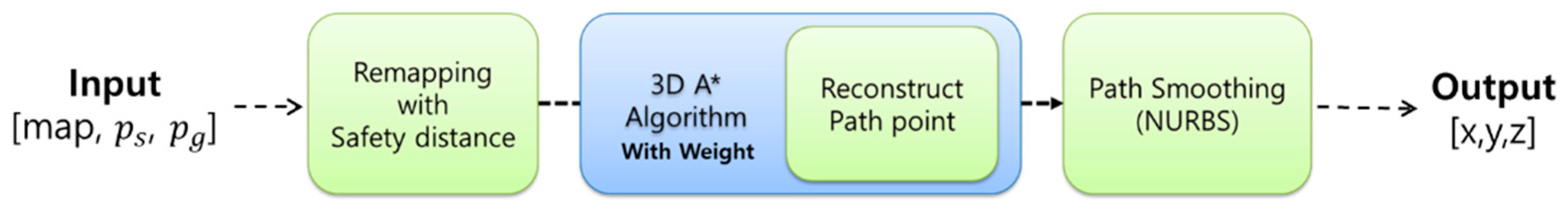
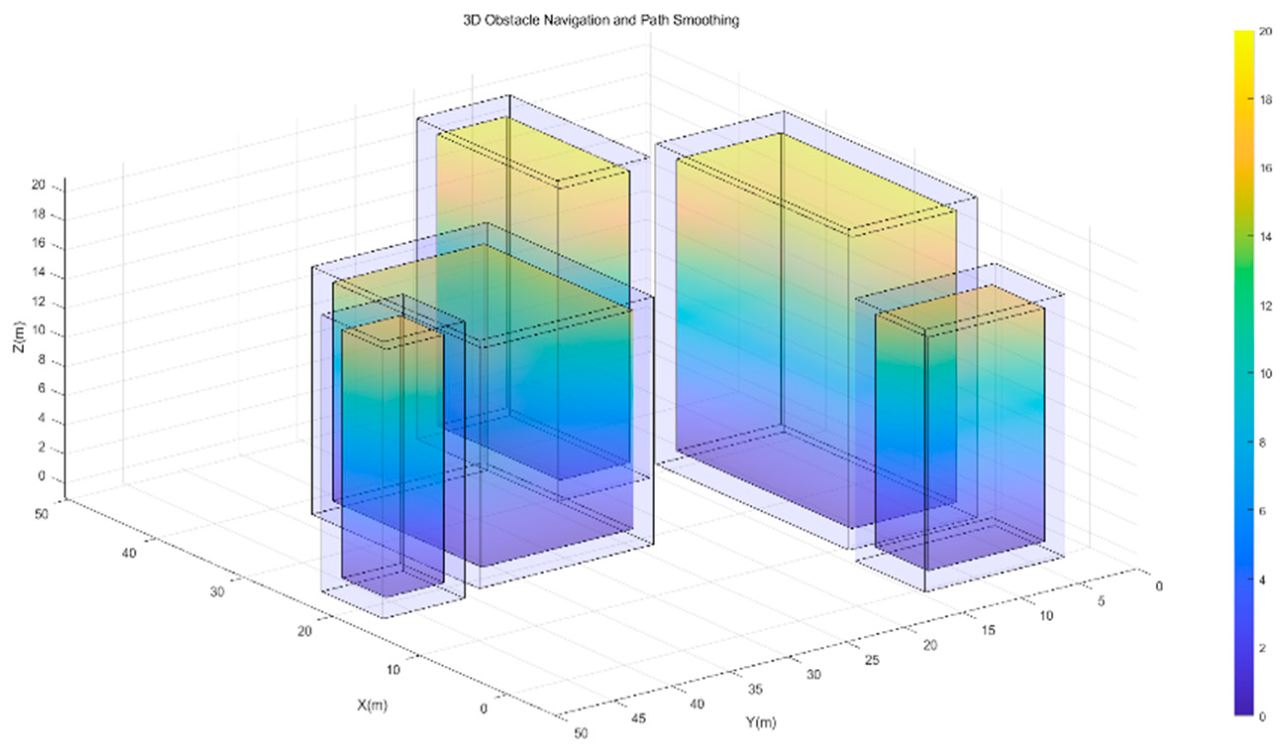
The overall structure of the proposed algorithm is shown in Figure 1. The algorithm takes the map information, a starting point, and a user-defined destination point as inputs. MATLAB/Simulink 2024a was used as the development platform, and the study was conducted under the assumption that map information is provided in the form of an occupancy grid map. The grid environment is a 60 × 50 × 20 m 3D map with a grid size of 1 m. Obstacles were modeled as rectangular prisms, representing urban buildings, and were randomly placed in positions that do not overlap with the start or destination points. The dimensions of the obstacles were set to be at least 5 m in the x and y directions and 12 m in the z direction.

The map size was fixed at 60 × 50 × 20, chosen to ensure consistent and fair comparisons. While it is true that computational time for grid-based algorithms increases linearly with map size, this study focuses on global path planning in a pre-mapped environment (e.g., cesium geospatial or building models), where the pre-planning approach is applicable. Furthermore, the heuristic-based nature of the algorithm ensures that the search for the optimal path remains unaffected by map size, even though larger maps may result in longer computation times. To maintain a manageable computational load and ensure reliable comparisons, the map size was fixed for all experiments.

The algorithm begins by generating a safety zone based on the given grid map, considering the UAV’s radius as shown in Figure 2. This ensures that the planned path does not come too close to obstacles. Using the map data, including the safety zones, the modified A* algorithm is executed to find a feasible path. The resulting path is then simplified using a path reduction algorithm, followed by a smoothing process to create a trajectory that the UAV can dynamically follow. Detailed designs of each module are described in the following sections.

2.1. Density-A* Algorithm

The A* algorithm, introduced by Nilsson in 1980, is a graph-based path-planning method designed to find the optimal path. It calculates the cost from the start to the goal node using an evaluation function that combines a heuristic (H-Cost) and actual cost (G-Cost). The algorithm prioritizes nodes using a priority queue, expanding those that minimize the evaluation function. It manages nodes with an open list for candidates and a closed list for fully explored nodes. The search ends when the goal node is reached or no further exploration is possible, producing the optimal path. The evaluation function is as follows:

$$f\left(n\right)=g\left(n\right)+h\left(n\right)$$

(1)

In the A* algorithm, the heuristic function is crucial for improving search efficiency. Its performance depends on how accurately it estimates the cost to the goal. Underestimating the heuristic can lead to inefficiently expanding the search space, while overestimating it can compromise the solution’s optimality. Thus, selecting a heuristic that closely approximates the actual cost is key.

Common heuristics include Euclidean, Manhattan, and Chebyshev distances. Euclidean distance provides accurate estimates for environments with unrestricted movement but may be less efficient in grids with limited horizontal or vertical movement. The calculations for these heuristics are as follows:

$$h{\left(n\right)}_{Euclidean}=\sqrt{{\left(x_g-x_c\right)}^2+{\left(y_g-y_c\right)}^2+{\left(z_g-z_c\right)}^2}$$

(2)

$$h{\left(n\right)}_{Manhattan}=abs\left(x_g-x_c\right)+abs\left(y_g-y_c\right)+abs\left(z_g-z_c\right)$$

(3)

$$h{\left(n\right)}_{Chebyshev}=Max\left[abs\left(x_g-x_c\right), abs\left(y_g-y_c\right),abs\left(z_g-z_c\right)\right]$$

(4)

where $\left(x_c,y_c,z_c\right)$ and $\left(x_g,y_g,z_g\right)$ denote current and goal nodes, respectively.

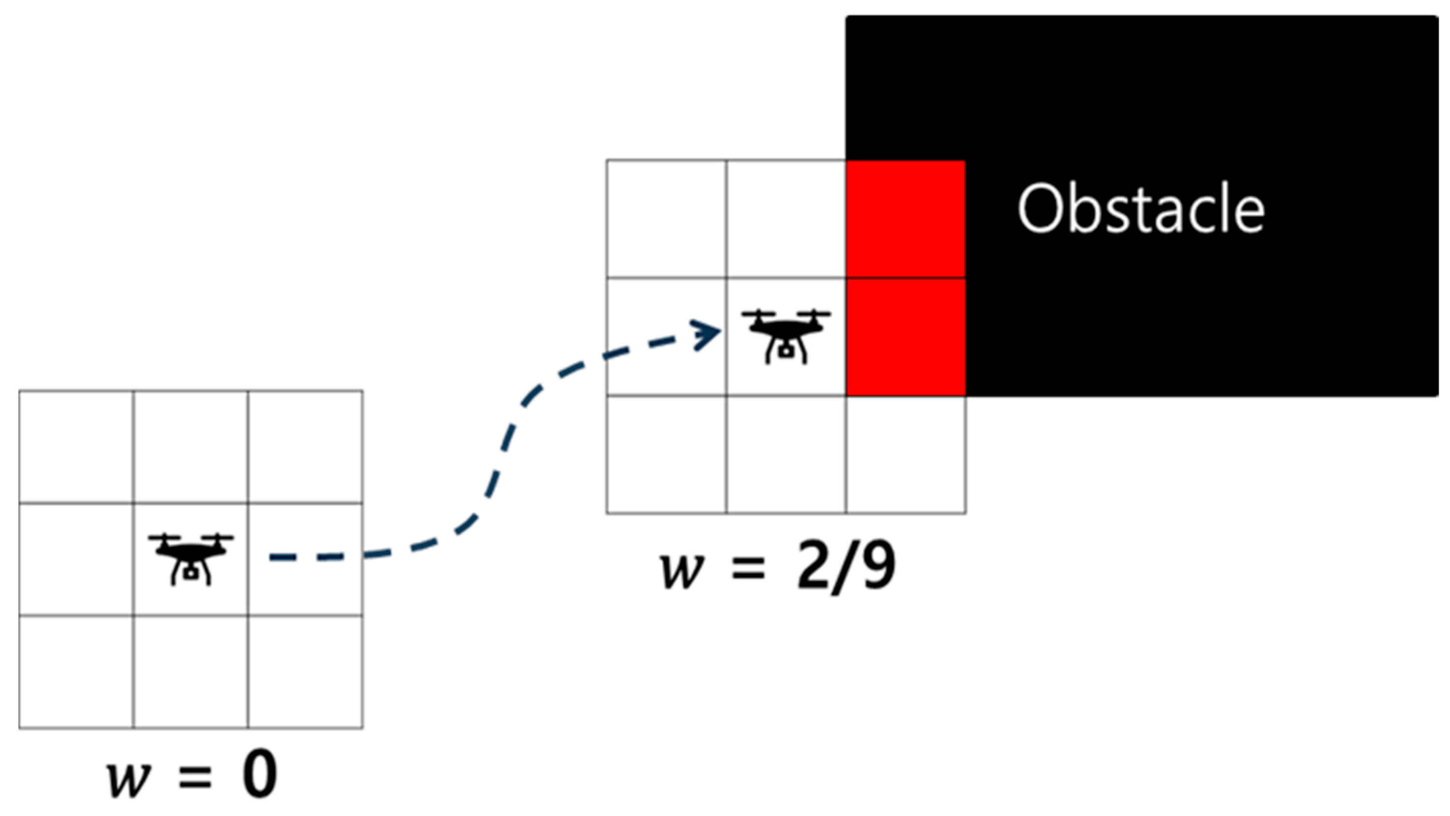
In DA*, the heuristic function incorporates local obstacle density to enable effective path planning in complex environments. The obstacle density, $d_{obs}$, is defined as a value between 0 and 1. As shown in Figure 3, $d_{obs}=0$ indicates no obstacles in the vicinity, while $d_{obs}$ approaching 1 signifies the surroundings are almost entirely obstructed. The density is computed for each node by dividing the number of cells occupied by obstacles within a 3 × 3 × 3 neighborhood by the total number of cells (26 in three-dimensional space).

Here, obstacle density quantitatively represents the distribution of obstacles around the current position, based on the occupancy of cells in the grid map. By offering more detailed local information during the path-planning process, obstacle density enhances both the efficiency and quality of the generated paths.

The final output of DA* is in the form of $\left(x,y,z,d_{obs}\right)$ with a size of N × 4, where N represents the length of the path. The additional $d_{obs}$ parameter, representing obstacle density at each node, provides valuable information for path optimization and ensures the generated trajectory accounts for environmental complexity. In this study, the Chebyshev distance was used as the base heuristic function. The Chebyshev distance is computationally efficient, as it selects the maximum travel distance among the axes, making it suitable for 3D spaces where diagonal movements frequently occur. However, relying solely on a distance-based heuristic can lead to inefficient paths, as it does not account for factors like obstacle density or energy consumption.

UAVs consume the most energy during altitude changes [27], with vertical ascents requiring over 20% more energy compared to horizontal or downward movements. Therefore, it is crucial to incorporate energy costs associated with vertical movements into path-planning algorithms. Additionally, the heuristic must encourage avoidance of areas with high obstacle density. To address these requirements, the final heuristic function was designed to include additional costs for altitude changes and obstacle density. The resulting heuristic function is as follows:

$$h\left(n\right)=h_{chebyshev}\left(n\right)+{\omega }_{alt}·\Delta z+{\omega }_{obs}·d_{obs}\left(n\right)$$

(5)

where ${\omega }_{alt}$ and ${\omega }_{obs}$ denotes the weight factor for altitude change costs and $\mathsf{\Delta }z$ is the difference in altitude relative to the goal. These parameters represent penalty weights for altitude changes and obstacle density, respectively, and are introduced to achieve the objective of minimizing altitude variations while avoiding regions with high obstacle density. In a conventional heuristic function, the cost is typically calculated based solely on the distance to the destination. However, in our study, the heuristic function was modified to include penalties for altitude changes and obstacle density. This ensures that even if the distance to the destination decreases, the cost will increase when moving to areas with significant altitude variations or high obstacle density.

The values of ${\omega }_{alt}$ and ${\omega }_{obs}$ were chosen empirically. For ${\omega }_{alt}$, setting the penalty too high could result in unnecessarily long detours, so careful consideration was given to strike a balance between minimizing altitude changes and maintaining path efficiency. Similarly, ${\omega }_{obs}$ was selected to prioritize obstacle avoidance without overly penalizing the path, while the specific values of 1.2 and 3 were determined based on experimental trials in simulation environments.

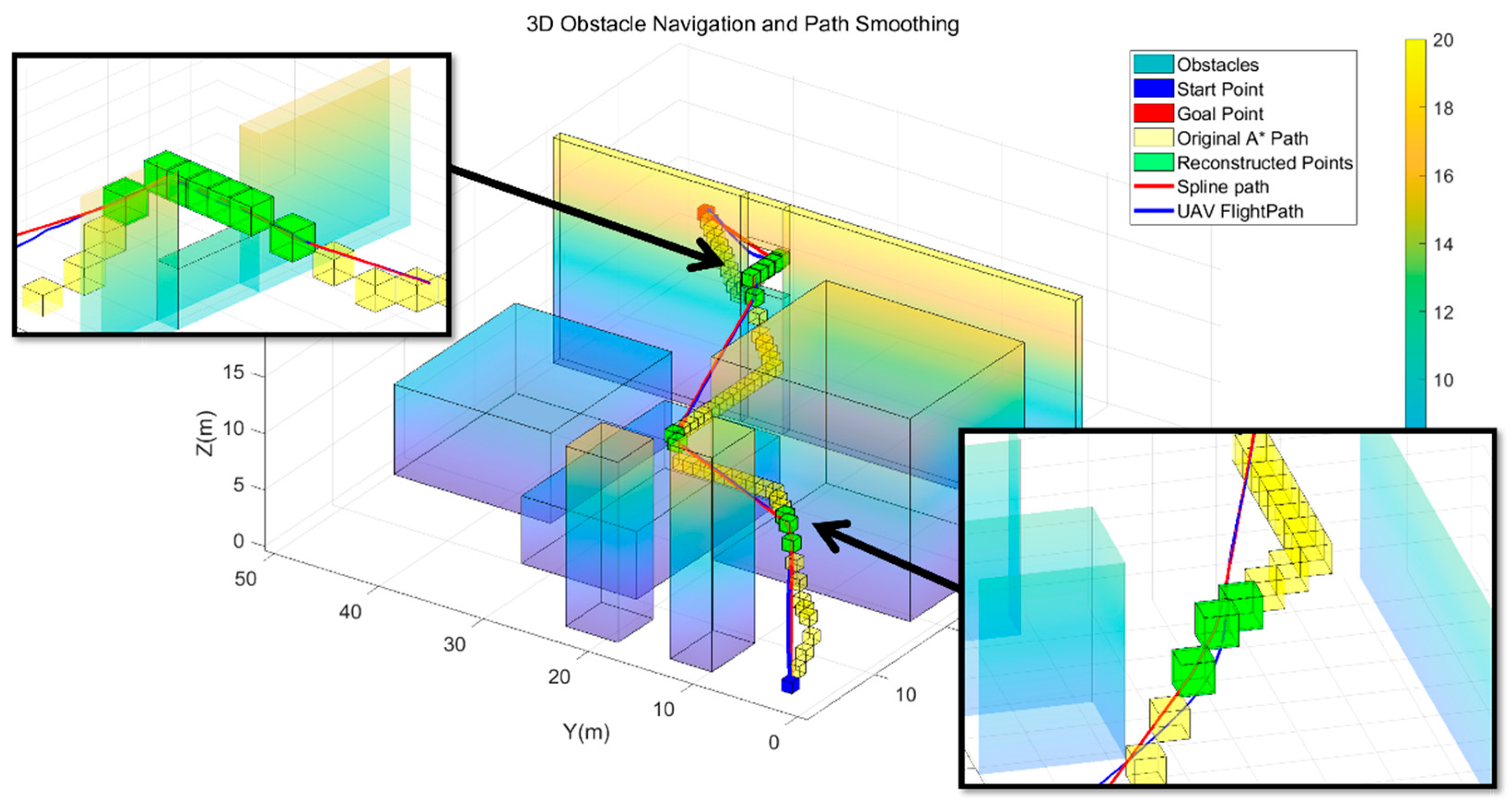
The comparison between the path generated by the proposed DA* algorithm with the designed heuristic function and the standard A* path is shown in Figure 4. The yellow path represents the standard A* algorithm using the Euclidean heuristic, while the green path represents the DA* algorithm incorporating obstacle density and altitude cost functions. As shown in the figure, the DA* path minimizes altitude changes and effectively avoids areas with high obstacle density, demonstrating the intended improvements.

2.2. Path Generator

2.2.1. Path Simplification Method

Path simplification is a crucial step in enhancing the efficiency and feasibility of the initial path generated by the planning algorithm. This process focuses on removing unnecessary nodes while maintaining the essential structure of the path required for safe obstacle avoidance. In this study, the simplification method combines obstacle density and geometric characteristics, such as angular changes, to selectively retain significant waypoints.

Nodes with obstacle density values exceeding a predefined threshold are included in the simplified path, as they represent areas with high obstacle density that require precise control and are thus critical. Additionally, nodes where the obstacle density transitions—either increasing from zero or decreasing to zero—are also retained. An increase indicates the first encounter with an obstacle, marking a critical transition point, while a decrease signifies exiting the obstacle region, ensuring the obstacle boundary is handled effectively during the smoothing process. Furthermore, nodes with significant angular changes between the previous and next nodes are preserved. Such changes reflect sharp directional adjustments, which are key geometric features of the path and must be maintained to preserve the overall structure and navigability.

The results of applying the path simplification algorithm are shown in Figure 5. Unlike the previous figure, the yellow cubes represent the initial path coordinates generated by the DA* algorithm, while the green cubes indicate the nodes after applying the simplification logic. The figure highlights the critical nodes selected based on changes in obstacle density, as well as those identified using thresholds for path angles and obstacle density. This approach ensures that the simplified path retains critical waypoints necessary for obstacle avoidance and efficient trajectory generation while reducing unnecessary complexity in less critical regions.

2.2.2. Path Smoothing Method

Path smoothing is an essential process to refine the simplified path generated after the initial planning phase. The goal is to produce a smooth and dynamically feasible trajectory that a UAV can follow efficiently. In this study, Non-Uniform Rational B-Splines (NURBS) interpolation is employed to smooth the path, ensuring continuity and smooth curvature while considering obstacle density and UAV maneuverability. NURBS uses the same basis functions as B-splines but assigns independent weights to each control point, allowing for more versatile curve representations. The position on the NURBS curve, $C\left(u\right)$, at a given parameter $u$, is calculated using the standard formulation, as shown in Equation (6) [28].

$$C\left(u\right)={\displaystyle \frac{{{\displaystyle \sum }}_{i=0}^n{N}_{i,k}\left(u\right){\omega }_i{P}_i}{{{\displaystyle \sum }}_{i=0}^n{N}_{i,k}\left(u\right){\omega }_i}}$$

(6)

where $P_i$ are the control points, ${\omega }_i$ are the weights assigned to each control point, and $n$ is the total number of control points. Here, the basis function $N_{i,k}\left(u\right)$ is calculated recursively based on the spline degree $k$ and the knot vector $u_i$, as follows:

$$N_{i,k}\left(u\right)={\displaystyle \frac{u-u_i}{u_{i+k}-u_i}}{N}_{i,k-1}\left(u\right)+{\displaystyle \frac{u_{i+k+1}-u}{u_{i+k+1}-u_{i+1}}}{N}_{i+1,k-1}\left(u\right)$$

(7)

NURBS, due to its high versatility and key characteristics, is widely used in various CAD and modeling applications where accuracy, flexibility, and computational efficiency are critical. These applications include tool path generation, vascular modeling, reverse engineering, and finite element analysis (FEM) [29,30].

Silva et al. implemented smooth and continuous 2D path smoothing for wheeled robots by applying NURBS weights selected as constant parameters, ensuring compliance with kinematic constraints [31]. Jalel et al. developed a multi-objective 2D path-planning method using NURBS weights based on path length, curvature metrics, and the number of control points [32].

However, existing studies have primarily focused on NURBS-based path interpolation in 2D environments, with limited application in 3D path planning. In 3D space, paths must account for both curvature and torsion, requiring the selection of interpolation weights that incorporate additional physical constraints. For UAV 3D path planning, it is essential to set appropriate weights for each path segment to meet requirements such as obstacle avoidance, energy efficiency, and control stability. In this study, the weights were determined as follows:

$${\omega }_i={\displaystyle \frac{\left(1-\alpha \right)·{\omega }_{low}+\alpha ·{\omega }_{high}}{d_{obs}+ϵ}}$$

(8)

where ${\omega }_{low}$ and ${\omega }_{high}$ represent the weights suitable for low-mobility and high-mobility UAVs, respectively. In this study, these were set to 0.5 and 10. $\alpha$ is the curvature index, which ranges between 0 and 1. A lower value indicates a low-mobility path, while higher values correspond to paths with greater curvature. $ϵ$ is a small arbitrary value added to avoid division by zero during calculations.

In the formula, the interpolation weights are set to be inversely proportional to obstacle density. This is because, during the path simplification process, all path points are retained in regions with high obstacle density, resulting in a larger number of control points. Therefore, it is unnecessary to assign high weights to areas with large $d_{obs}$. Instead, higher weights are required for control points at obstacle corners where $d_{obs}$ is smaller, ensuring smoother transitions and better handling of critical path segments. 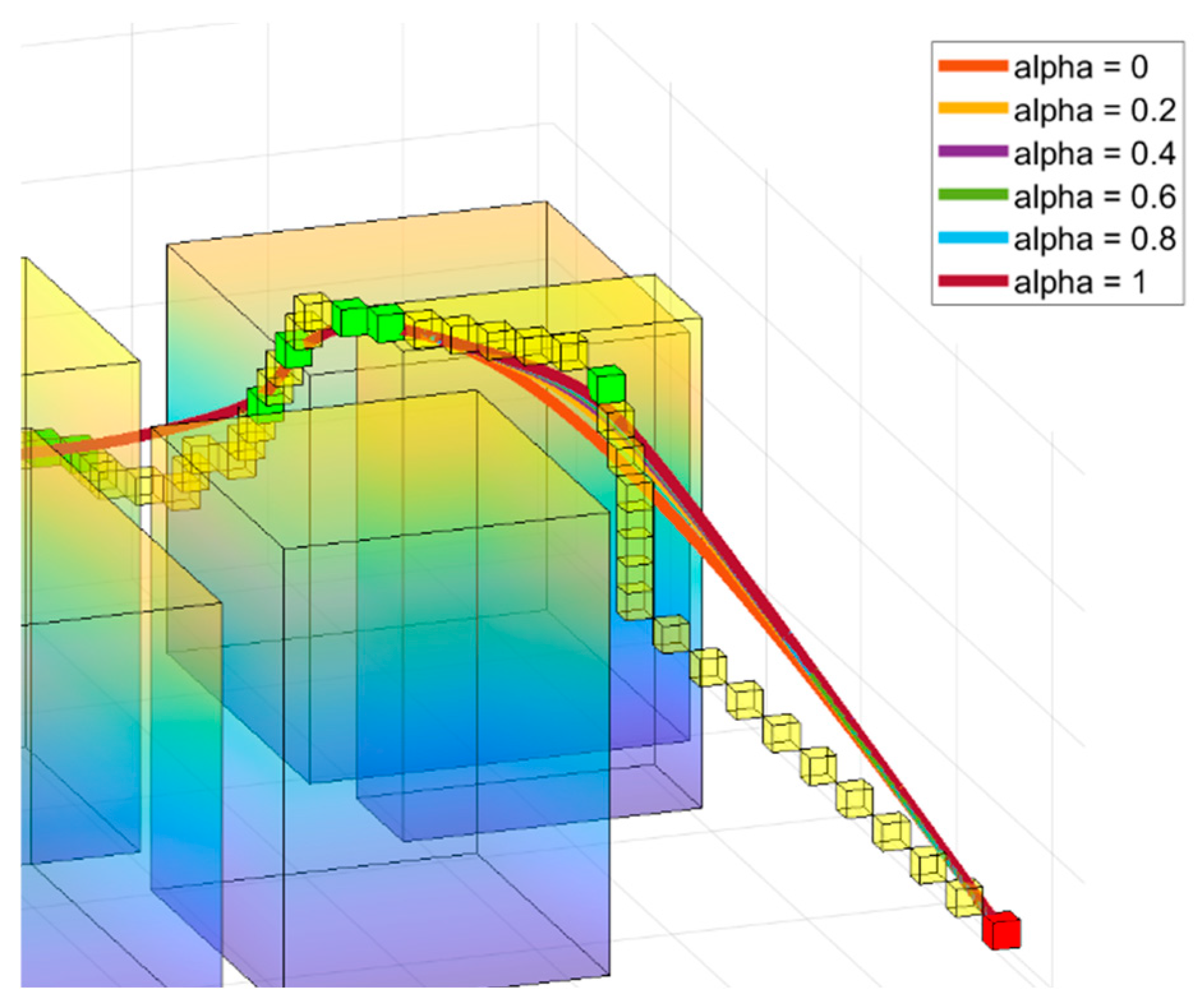The interpolated path with applied weights is shown in Figure 6.

However, the comparison of paths based on different $\alpha$ values is shown in Figure 7. When $\alpha$ is small, the interpolation weights decrease, resulting in minimized curvature and smoother paths. As $\alpha$ increases, the curvature becomes larger, enabling quicker direction changes and sharper maneuvers. This demonstrates that if a path overlaps with obstacles, $\alpha$ can be increased to re-interpolate the path, allowing for effective path verification and adjustment l.

2.3. Path-Planning Result

The parameters used in the algorithm are summarized in

Table 1. Path-planning algorithm parameters.

Classification	Parameter	Value
Initial input	Map size [x, y, z] (m)	[20, 50, 60]
	Grid size (m)	1
DA*	${\omega }_{alt}$	1.2
	${\omega }_{obs}$	3
NURBS	${\omega }_{low}$	0.5
	${\omega }_{high}$	10

. The initial path generated by the DA* algorithm effectively integrated obstacle density and altitude costs, avoiding areas with high obstacle density and minimizing unnecessary altitude changes. After applying the path simplification and smoothing processes, the final trajectory was optimized for UAV navigation. The simplified path retained critical waypoints while eliminating redundant nodes, and the smoothed trajectory ensured continuous curvature and dynamic feasibility, meeting the operational requirements of UAVs in complex 3D environments. Figure 8, Figure 9 and Figure 10 illustrate the results of algorithm execution across various environments.

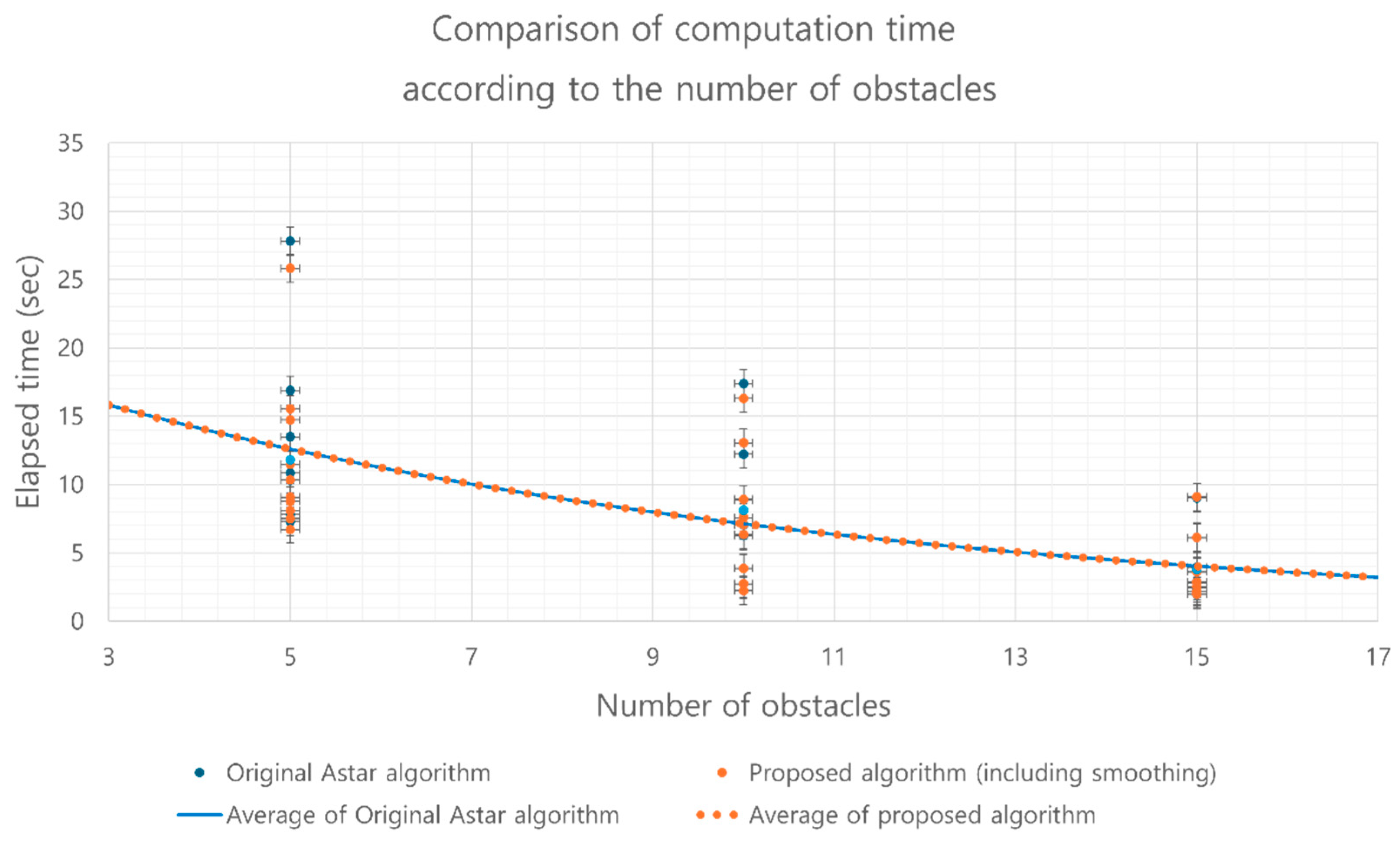
Figure 11 compares the computational speed of the proposed algorithm with that of the conventional A* algorithm under varying obstacle densities. The results show that the proposed algorithm achieves computational costs comparable to the conventional A* algorithm, even with the addition of the path interpolation process. When evaluated in identical map environments and using the same algorithm parameters, the proposed algorithm demonstrated nearly identical computational speeds. Both algorithms also displayed a consistent trend of reduced search time as the number of obstacles increased. This trend can be attributed to the confined map size, where higher obstacle densities limit the number of feasible paths, thereby shortening the search process.

The numerical average results of path comparisons, obtained through Monte-Carlo simulations over 100 random maps for each obstacle count, are summarized in

Table 2. Algorithm performance based on number of obstacles.

No. of Obstacles	Elapsed Time (Sec)			Path Reduction Rate (%)
	Min.	Max.	Avg.	Min.	Max.	Avg.
5	2.00	55.00	20.00	3.4	9.8	7.2
10	1.30	21.00	8.00	2.2	11.0	6.8
15	0.86	16.17	5.18	3.0	11.6	6.2

. Although computational speed varied significantly depending on the map configuration, a consistent trend was observed: as the number of obstacles increased, the number of search nodes decreased, leading to shorter computation times. In terms of path reduction, the proposed algorithm achieved an approximate 7% reduction in path length across all obstacle densities, attributed to the path smoothing process.

3. Simulation

3.1. Quadcopter Dynamics Modeling

The dynamic behavior of the unmanned aerial vehicle (UAV) was simulated using the Guidance Model provided by UAV Toolbox [33]. This model incorporates a pre-configured attitude controller and simplified dynamic equations to approximate UAV motion, ensuring computational efficiency and stability during simulation. The Guidance Model allows for the simulation of multirotor UAVs with inputs for roll, pitch, yaw rate, and thrust commands. These features provided a reliable foundation for evaluating the performance of the proposed path-planning algorithm.

The attitude controller within the Guidance Model was used to track the reference waypoints generated by the proposed path-planning algorithm. The model’s built-in control logic was validated in previous studies and industry applications, making it suitable for ensuring realistic UAV behavior during simulation [34,35,36,37,38]. The tool was used without modification, and its standard parameters were adopted unless otherwise stated.

3.2. Trajectory Following

The interpolated path generated by the algorithm consists of a list of position coordinates. However, directly using these coordinates as the UAV’s flight path can lead to issues. When velocity commands are generated based on position errors, the small spacing between the interpolated path points results in minimal position errors, causing the UAV to move unnecessarily slowly. As a result, the UAV may exhibit inefficient flight behavior, such as excessive deceleration or repeated acceleration and deceleration while following the target path. These stepwise velocity commands can degrade the smoothness and stability of the UAV’s flight.

Smooth and efficient following of the interpolated path requires a Trajectory Following logic. This logic generates velocity and direction commands that consider the UAV’s kinematic constraints and dynamic characteristics, enabling stable and natural flight. In this study, a triplet structure was used for trajectory following, consisting of the previous, current, and next target waypoints. The linear velocity for each waypoint was calculated based on the position error between the UAV and the respective waypoint. Specifically, the velocity for the current waypoint was determined using the position error between the UAV and the current target, while the velocity for the next waypoint was calculated based on the position error between the UAV and the next target. These two velocities were blended using weighting factors to produce the final velocity command.

To achieve smooth transitions, the weight assigned to the next waypoint was gradually increased as the UAV approached the current waypoint. This method prevented excessive deceleration or halting at waypoints, ensuring seamless and natural progression to the next target. Additionally, the final velocity command was constrained to remain within the UAV’s maximum speed limit, ensuring both safe and efficient operation. The final linear velocity calculation is expressed as follows:

$${\omega }_{current}=Max\left(0.5, 1-{\displaystyle \frac{D_{current}}{r_{reach}}}\right), {\omega }_{next}=1-{\omega }_{current}$$

(9)

$$v_{combined}={\omega }_{current}·v_{current}+{\omega }_{next }·v_{next}$$

(10)

$$v_{final}=\left\{\begin{array}{cc}\hfill v_{combined},& \left|\left|v_{combined}\right|\right|\le v_{max}\hfill \\ \hfill v_{combined}·{\displaystyle \frac{v_{max}}{\left|\left|v_{combined}\right|\right|}},& \left|\left|v_{combined}\right|\right|v_{max}\hfill \end{array}\right.$$

(11)

In this equation, ${\omega }_{current}$ represents the weight for the current waypoint and is defined as the ratio of the distance $D_{current}$ to the threshold distance $r_{reach}$ which determines waypoint proximity. ${\omega }_{next}$ presents the weight for the next waypoint and is calculated such that it gradually increases as the UAV approaches the current waypoint. Figure 12 shows the trajectory following module implemented in Simulink.

The generated velocity commands are fed into a velocity controller structured with a PID loop. The controller’s output (acceleration) is combined with gravity and converted into attitude command values. The attitude commands are fed into the Quadcopter Dynamics Model, which ultimately calculates the current position, velocity, Euler angles, and angular velocity. The final selected key parameters for the outer loop controller are shown in

Table 3. Controller gains.

Controller	Parameter	Value
Position control (trajectory following)	$r_{reach}$	2
	$v_{max}$	5
	$K_p^{POS}$	0.7
Velocity control	$K_p^{POS}$	0.08
	$K_i^{POS}$	0.01
	$K_d^{POS}$	0.01

.

4. Simulation Result

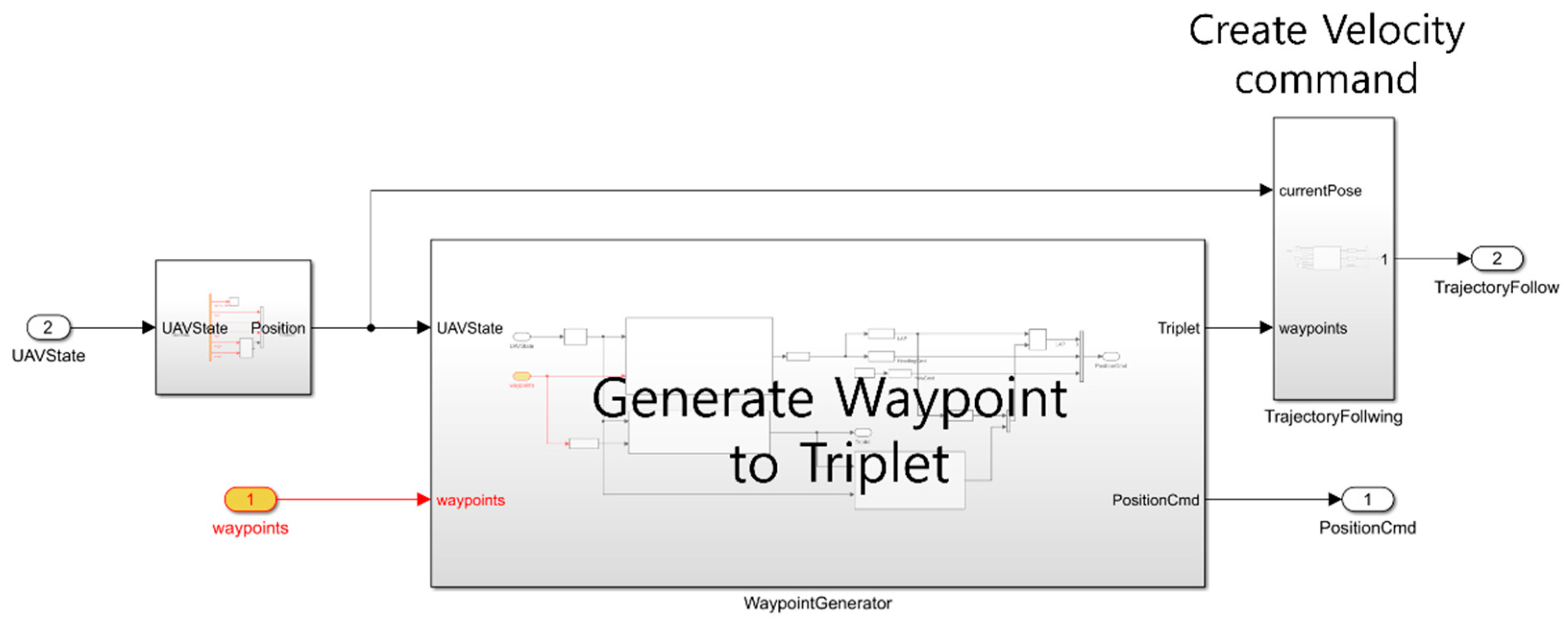
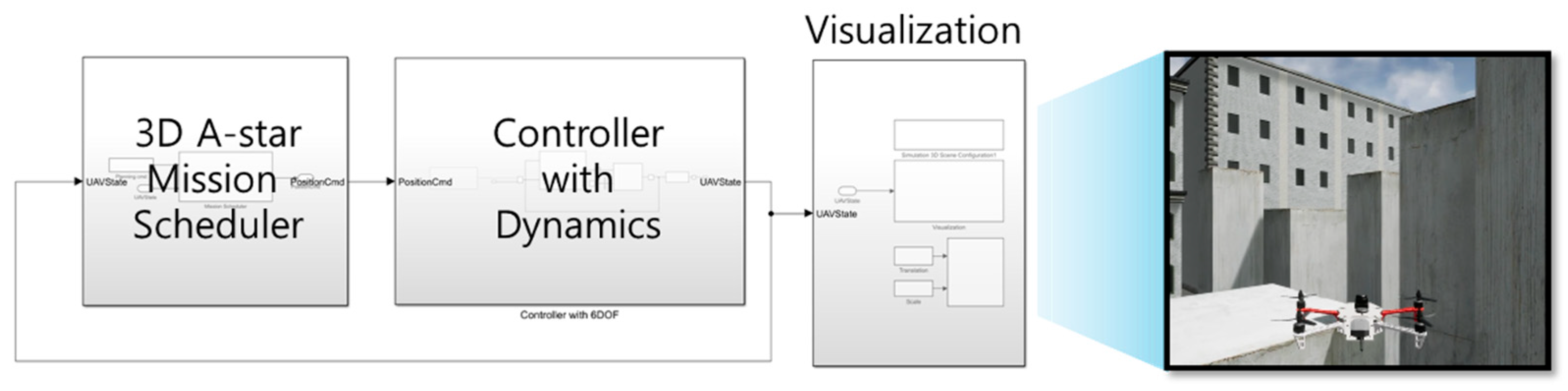
In the Simulink simulation, the system is organized into three main modules, as shown in Figure 13. The first module runs the designed A* algorithm and path interpolation. It schedules path planning based on the UAV’s current state feedback to generate position commands. The second module is the dynamics module, which includes controllers. It consists of a dual PID control loop for position/velocity control and uses an approximate dynamics model, including the attitude controller, to compute the UAV’s current position and orientation. Finally, the visualization module integrates with Unreal Engine to display obstacle and UAV position information based on the current state of the UAV.

The UAV’s flight trajectory obtained from simulations is shown alongside the algorithm-generated path in Figure 14 and Figure 15. It was confirmed that the proposed algorithm successfully tracks the path within a margin of 0.5 m across various environments. Even in areas with high obstacle density, the UAV reliably followed the path and reached the target destination. These results demonstrate the reliability of the proposed algorithm.

The qualitative performance comparison of the algorithms in identical map environments is presented in

Table 4. Performance comparison between A* and the proposed algorithm.

Metric	Original A*	DA*
Distance (m)	98.69	91.76
Reach time (s)	280.98	249.77
Max velocity (m/s)	1.38	2.71
Average velocity (m/s)	0.36	0.89

. The proposed algorithm generates continuous and dynamically feasible paths, minimizing deceleration segments. As a result, while the difference in travel distance is within approximately 5%, the proposed algorithm reduces arrival time by 10–15%, demonstrating improved performance.

5. Discussion

The experimental results highlight the proposed algorithm’s ability to balance computational efficiency and path quality, even in obstacle-dense environments. Compared to traditional A* algorithms, the integration of local obstacle density into the heuristic function significantly improves navigation in urban and industrial settings. Additionally, the use of NURBS interpolation ensures smooth and dynamically feasible trajectories, reducing travel time by more than 10%.

Despite its strengths, the algorithm has certain limitations. Currently, it focuses solely on global path planning and does not account for dynamic obstacles, which are critical in real-world applications. Additionally, the computational time increases linearly with the map size, which poses a scalability challenge. For instance, on a 100 × 100 × 20 grid map, the algorithm’s runtime was measured at 264 s. Addressing these issues will be essential for enhancing the practicality of the algorithm in larger and more complex environments. Addressing dynamic obstacles will require the integration of this approach with local planners, such as Rapidly-exploring Random Trees (RRT), Dynamic Window Approach (DWA), and Artificial Potential Fields (APF). Future research will focus on integrating this approach with local planners to enhance its applicability in dynamic and highly complex environments.

6. Conclusions

As UAVs become increasingly utilized, autonomous flight in complex environments, such as urban areas, is critical for their practical deployment. Current path-planning technologies focus heavily on two-dimensional algorithms, while existing three-dimensional approaches often lack effectiveness in dense, obstacle-rich settings. To address these challenges, we propose the Density-A* algorithm, an extension of the A* algorithm tailored for 3D path planning in complex environments.

The Density-A* algorithm incorporates local obstacle density storage for each node, facilitating efficient path simplification and interpolation to produce smooth, UAV-friendly trajectories. Numerical simulations in various scenarios demonstrated the algorithm’s capability to remove unnecessary nodes and create optimized paths by leveraging obstacle density and path angle information. Validation through quadcopter dynamic simulations confirmed the UAV’s ability to follow generated paths with high precision, achieving a reduction in travel time by over 10% compared to conventional approaches.

This study highlights the integration of local obstacle density into the A* algorithm, enabling efficient 3D path-planning suitable for UAV applications in complex environments. Future research will focus on integrating this approach with real-time local path planning methods and multi-UAV coordination to further enhance its applicability and scalability in dynamic, real-world scenarios.