Author Contributions
Conceptualization, S.D., T.S. and J.F.W.; methodology, S.D.; software, S.D.; validation, S.D.; formal analysis, S.D.; investigation, S.D.; resources, S.D., T.S. and J.F.W.; data curation, S.D.; writing—original draft preparation, S.D.; writing—review and editing, T.S. and J.F.W.; visualization, S.D.; supervision, T.S. and J.F.W. All authors have read and agreed to the published version of the manuscript.
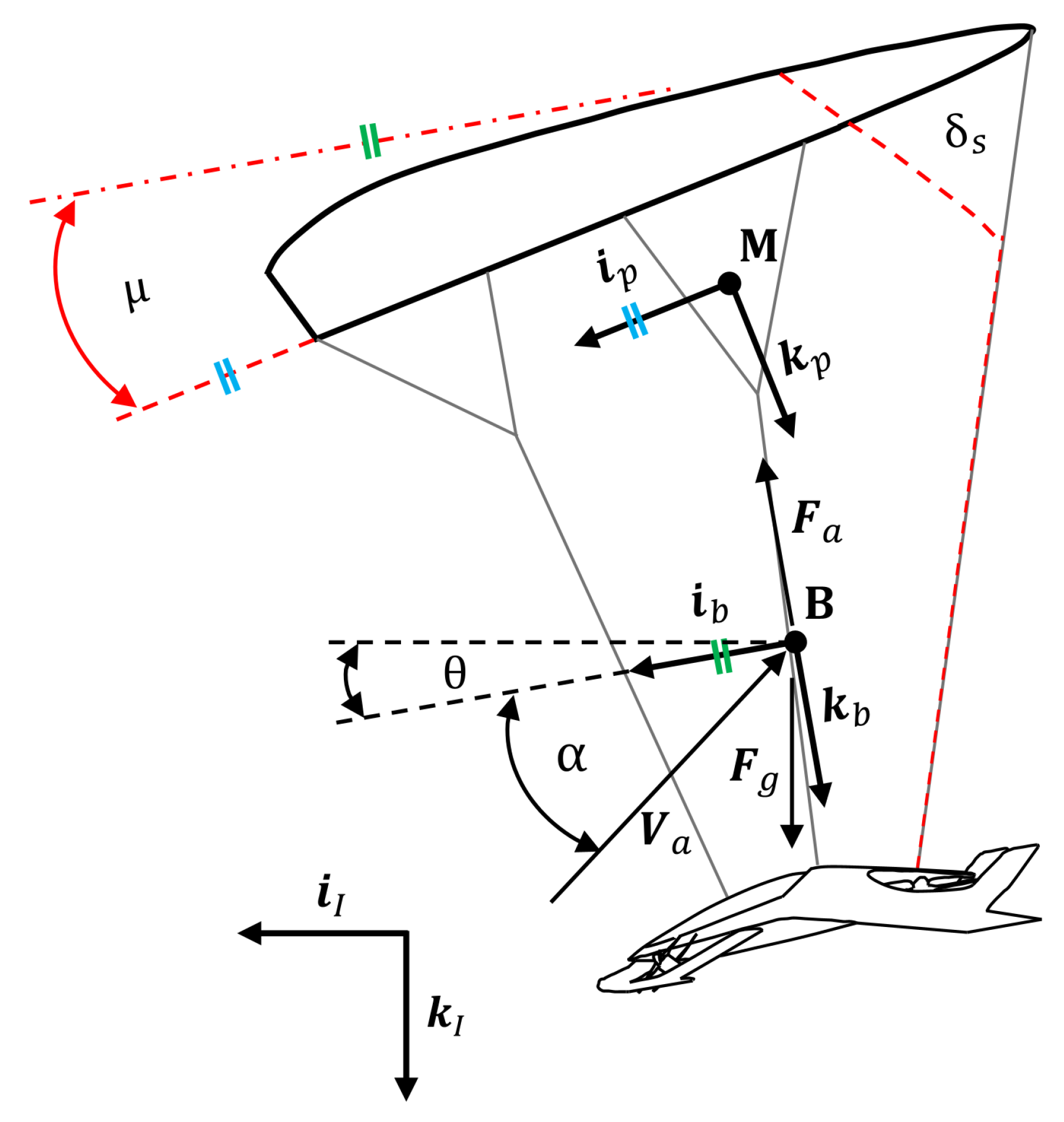
Figure 1.
Six-DOF parafoil and eVTOL payload system free body diagram.
Figure 1.
Six-DOF parafoil and eVTOL payload system free body diagram.
Figure 2.
The Aston Martin Volante Vision concept eVTOL aircraft.
Figure 2.
The Aston Martin Volante Vision concept eVTOL aircraft.
Figure 3.
Simulink implementation of six-DOF model.
Figure 3.
Simulink implementation of six-DOF model.
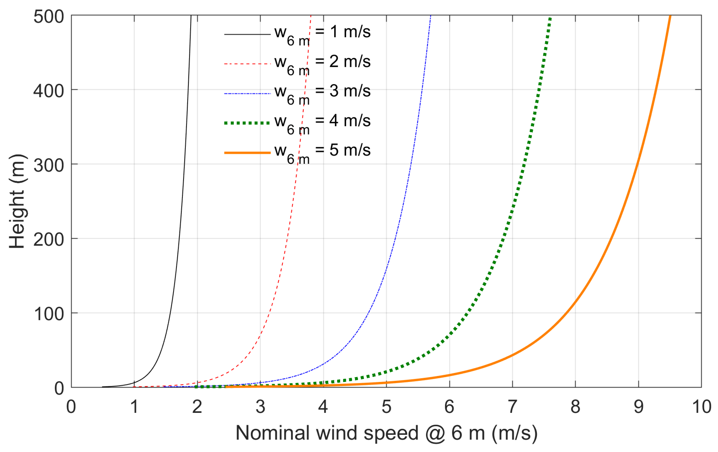
Figure 4.
Wind shear visualisation for heights of 0–500 m and horizontal wind speeds at 6 m of 1–5 m/s.
Figure 4.
Wind shear visualisation for heights of 0–500 m and horizontal wind speeds at 6 m of 1–5 m/s.
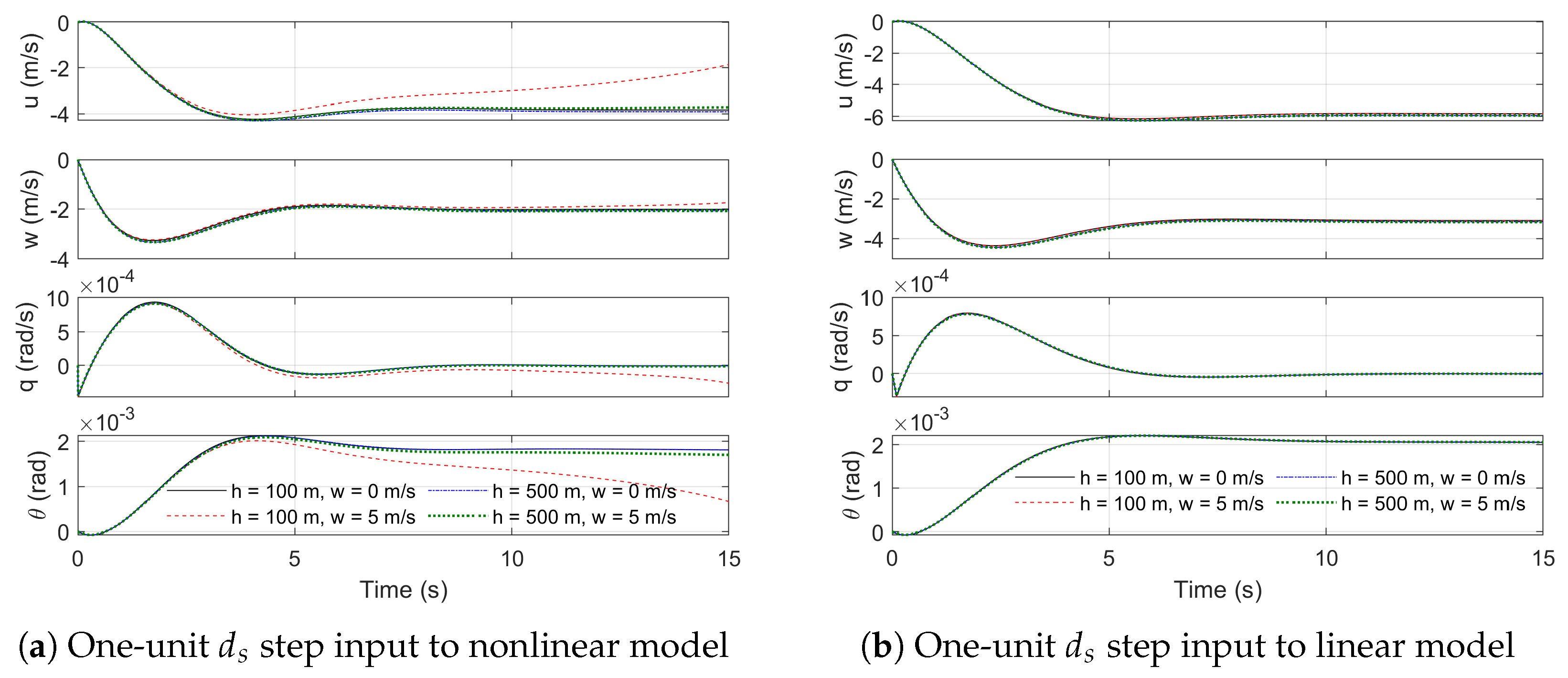
Figure 5.
Nonlinear and linear models response to 1 unit step control input at various heights and nominal wind conditions at 6 m.
Figure 5.
Nonlinear and linear models response to 1 unit step control input at various heights and nominal wind conditions at 6 m.
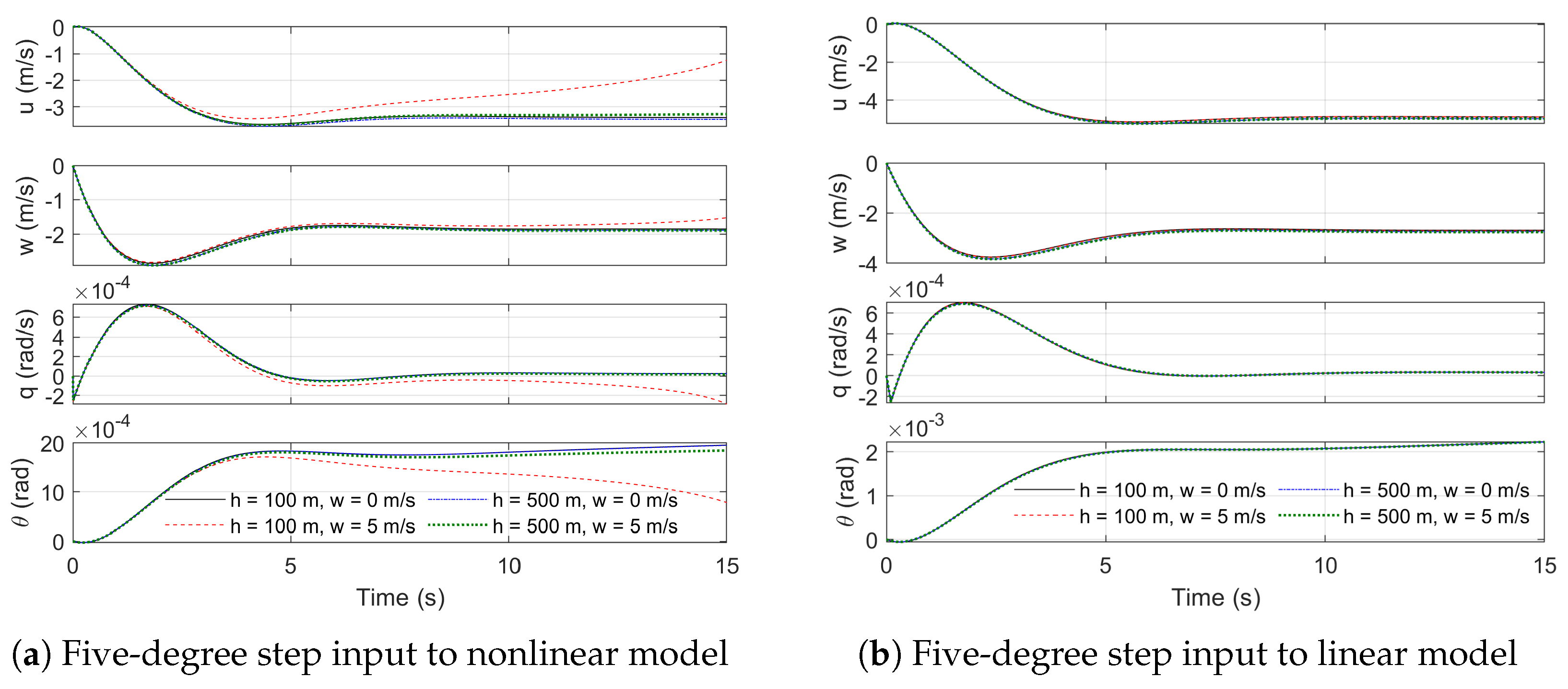
Figure 6.
Nonlinear and linear models response to step control input at various heights and nominal wind conditions at 6 m.
Figure 6.
Nonlinear and linear models response to step control input at various heights and nominal wind conditions at 6 m.
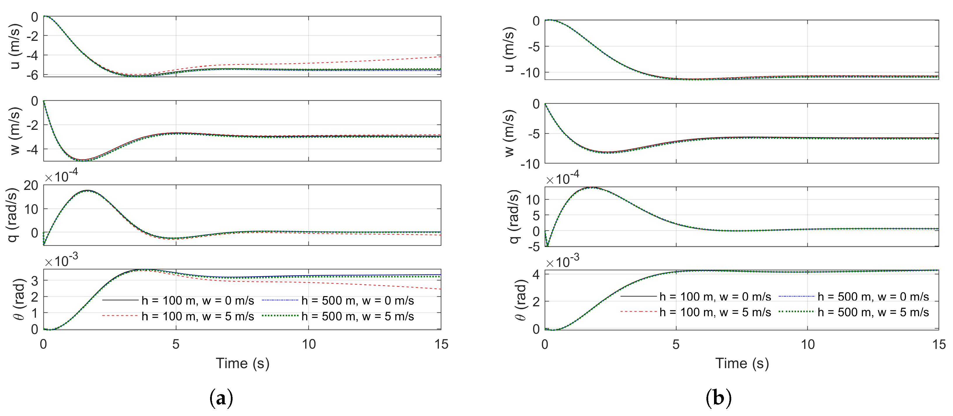
Figure 7.
Nonlinear and linear models response to step control input at various heights and nominal wind conditions at 6 m. (a) Combined 1-unit and step input to nonlinear model. (b) Combined 1-unit and step input to linear model.
Figure 7.
Nonlinear and linear models response to step control input at various heights and nominal wind conditions at 6 m. (a) Combined 1-unit and step input to nonlinear model. (b) Combined 1-unit and step input to linear model.
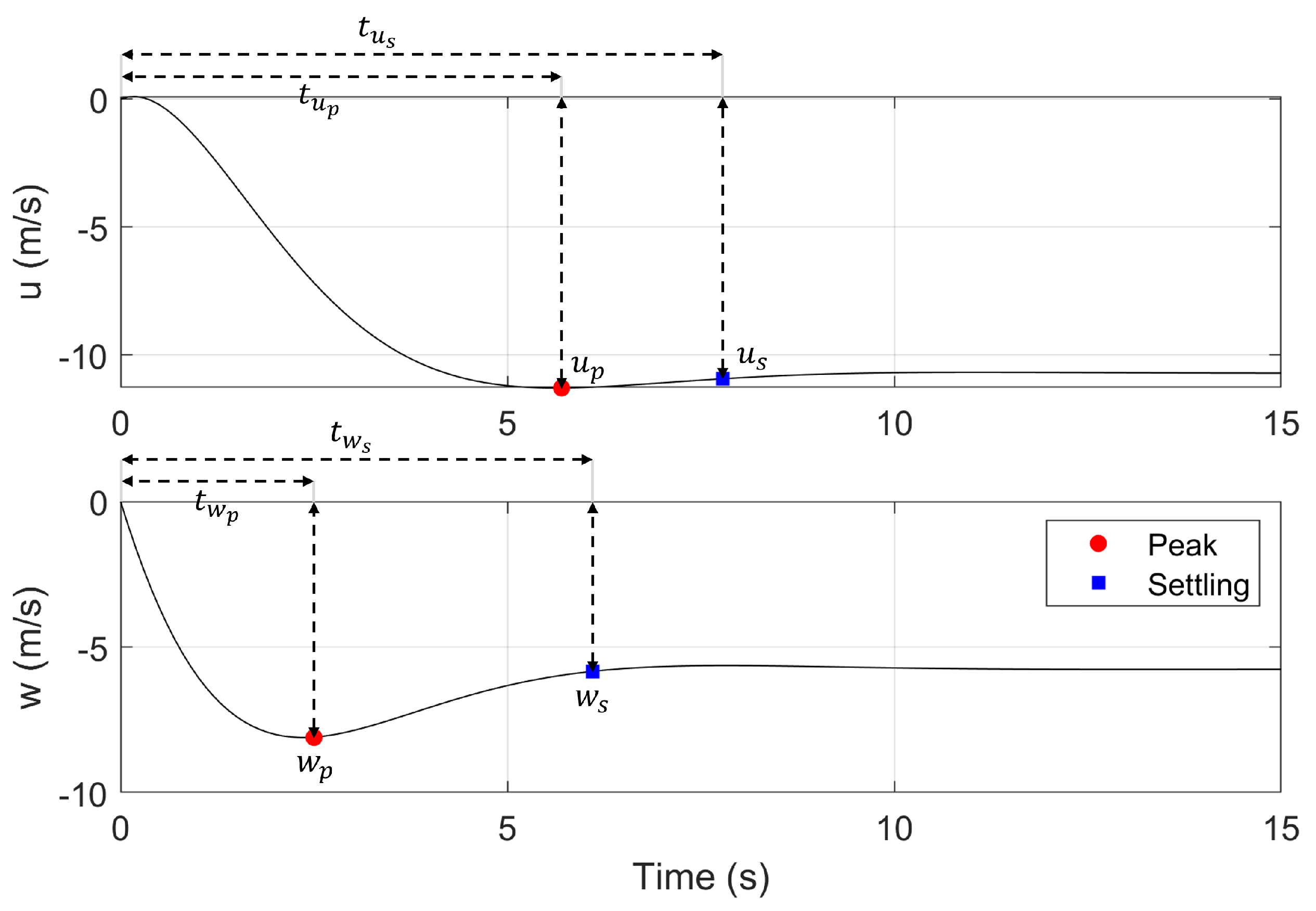
Figure 8.
Combined 1-unit and step response metrics and a height of 100 m and nominal wind speed at 6 m of 0 m/s.
Figure 8.
Combined 1-unit and step response metrics and a height of 100 m and nominal wind speed at 6 m of 0 m/s.
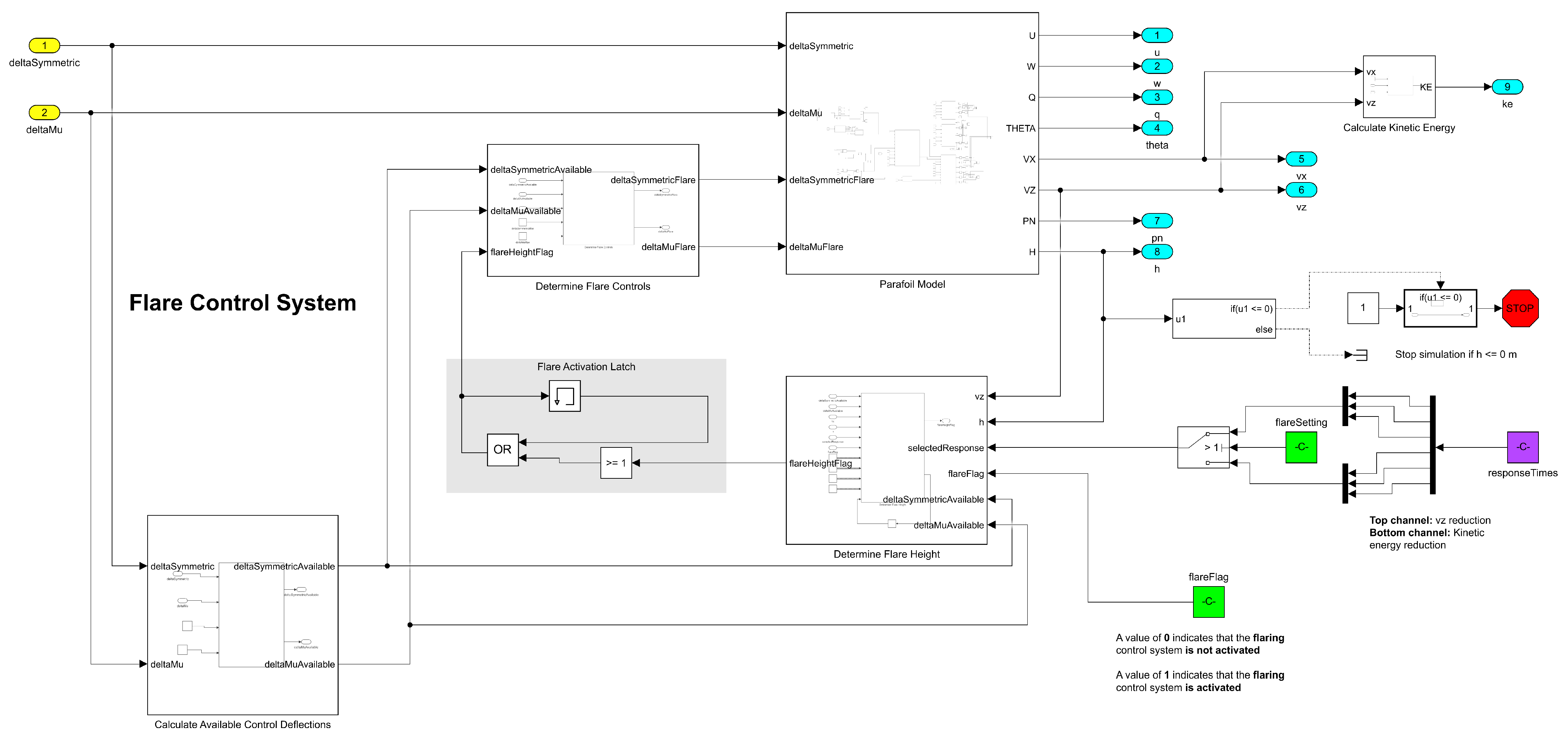
Figure 9.
Simulink implementation of inner-loop flare controller.
Figure 9.
Simulink implementation of inner-loop flare controller.
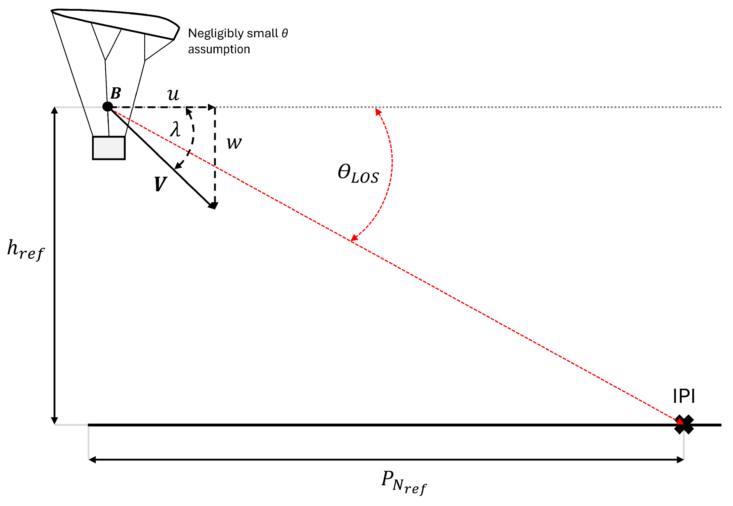
Figure 10.
Standard longitudinal line-of-sight guidance method.
Figure 10.
Standard longitudinal line-of-sight guidance method.
Figure 11.
Relationship between prediction horizon and IPI-targeting behaviour of a parafoil and eVTOL payload system.
Figure 11.
Relationship between prediction horizon and IPI-targeting behaviour of a parafoil and eVTOL payload system.
Figure 12.
Adaptive longitudinal line-of-sight guidance method.
Figure 12.
Adaptive longitudinal line-of-sight guidance method.
Figure 13.
Full control system architecture.
Figure 13.
Full control system architecture.
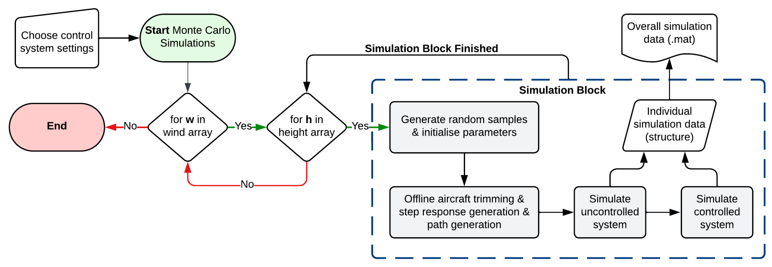
Figure 14.
Monte Carlo simulation flowchart.
Figure 14.
Monte Carlo simulation flowchart.
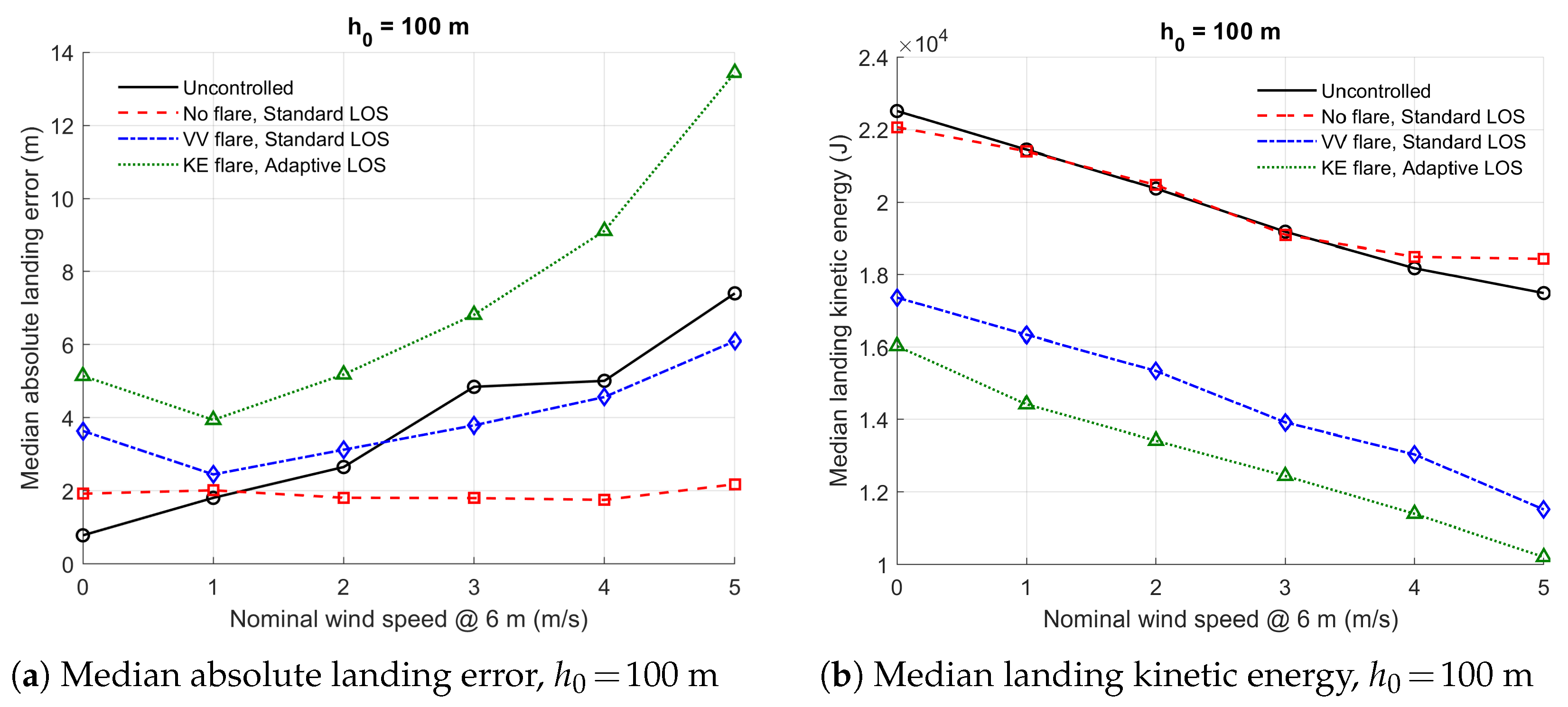
Figure 15.
Median absolute landing error and landing kinetic energy comparison for m.
Figure 15.
Median absolute landing error and landing kinetic energy comparison for m.
Figure 16.
Median absolute landing error and landing kinetic energy comparison for m.
Figure 16.
Median absolute landing error and landing kinetic energy comparison for m.
Figure 17.
Median absolute landing error and landing kinetic energy comparison for m.
Figure 17.
Median absolute landing error and landing kinetic energy comparison for m.
Figure 18.
Landing position of system with vertical velocity reduction flare setting and standard LOS guidance and system with kinetic energy reduction flare setting and adaptive LOS guidance. Nominal wind speed at 6 m of 2 m/s. (a) Vertical velocity reduction flare setting and standard LOS guidance. (b) Kinetic energy reduction flare setting and adaptive LOS guidance.
Figure 19.
Landing position of system with vertical velocity reduction flare setting and standard LOS guidance and system with kinetic energy reduction flare setting and adaptive LOS guidance. Nominal wind speed at 6 m of 0 m/s. (a) Vertical velocity flare setting and standard LOS guidance. (b) Kinetic energy reduction flare setting and adaptive LOS guidance.
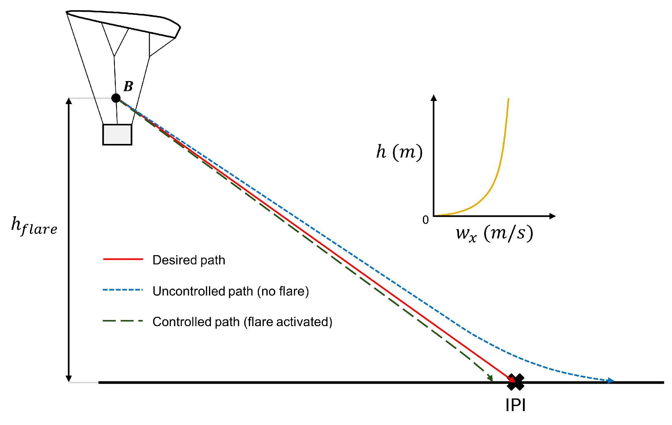
Figure 20.
Comparison of system path loci during flaring with and without the flare control system activated.
Figure 20.
Comparison of system path loci during flaring with and without the flare control system activated.
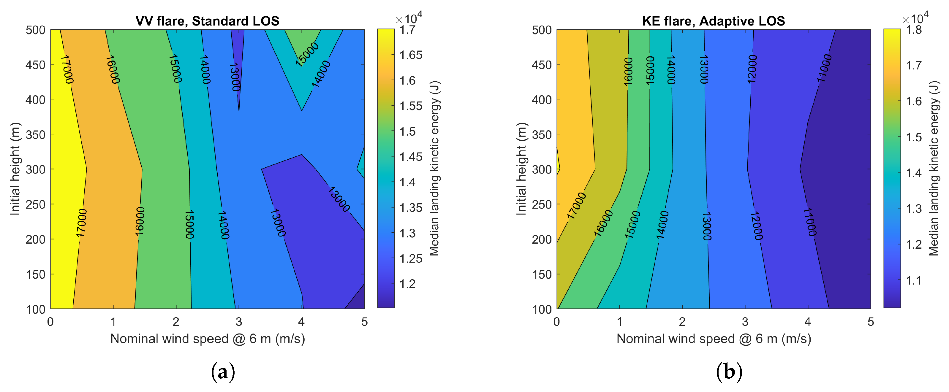
Figure 21.
Landing kinetic energy contour plots for system with vertical velocity reduction flare setting and standard LOS guidance and system with kinetic energy reduction flare setting and adaptive LOS guidance. (a) Vertical velocity reduction flare setting and standard LOS guidance. (b) Kinetic energy reduction flare setting and adaptive LOS guidance.
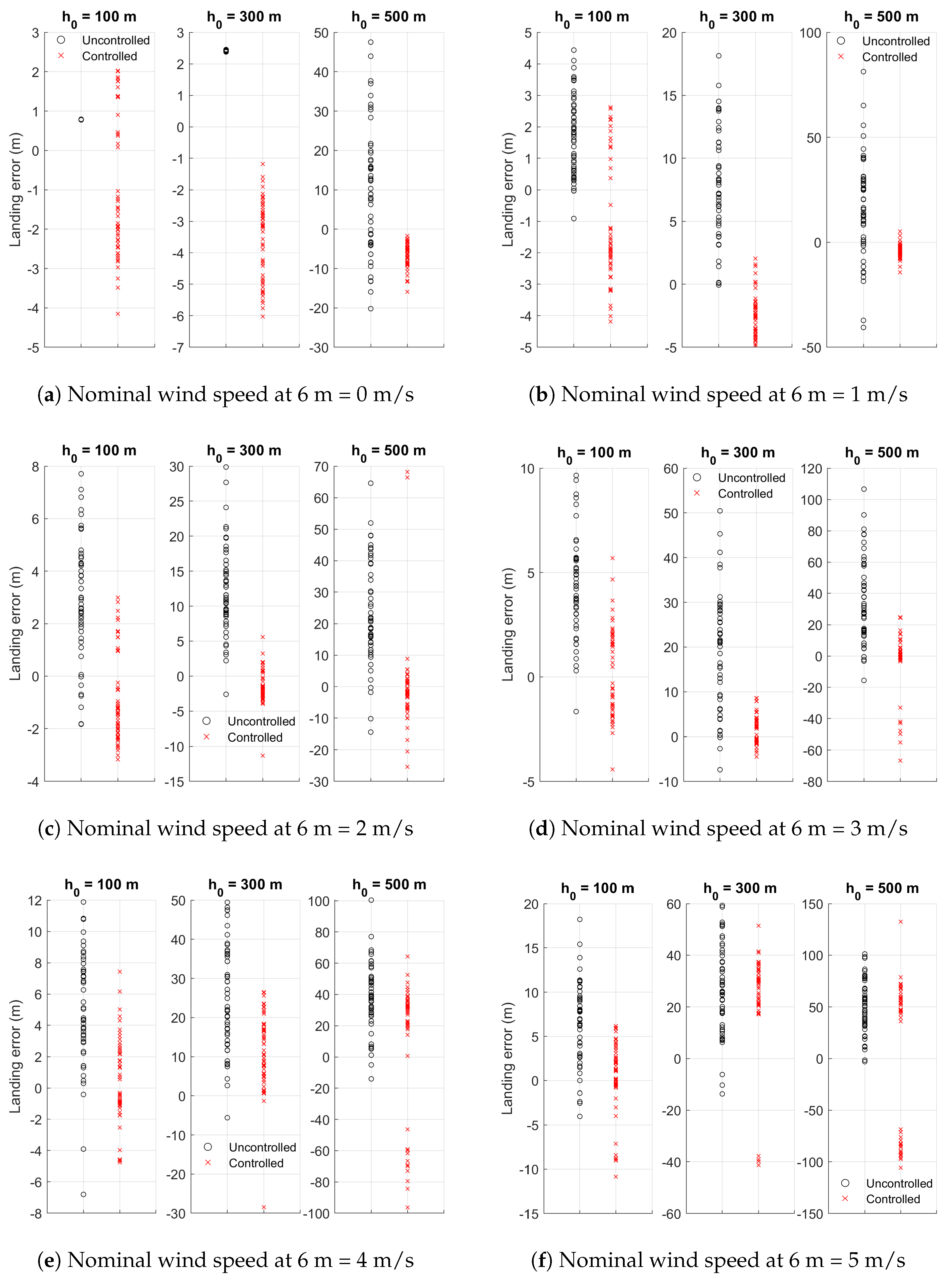
Figure 22.
Landing error of system with no flare setting and standard LOS guidance at nominal wind speeds at 6 m of 4 m/s and 5 m/s.
Figure 22.
Landing error of system with no flare setting and standard LOS guidance at nominal wind speeds at 6 m of 4 m/s and 5 m/s.
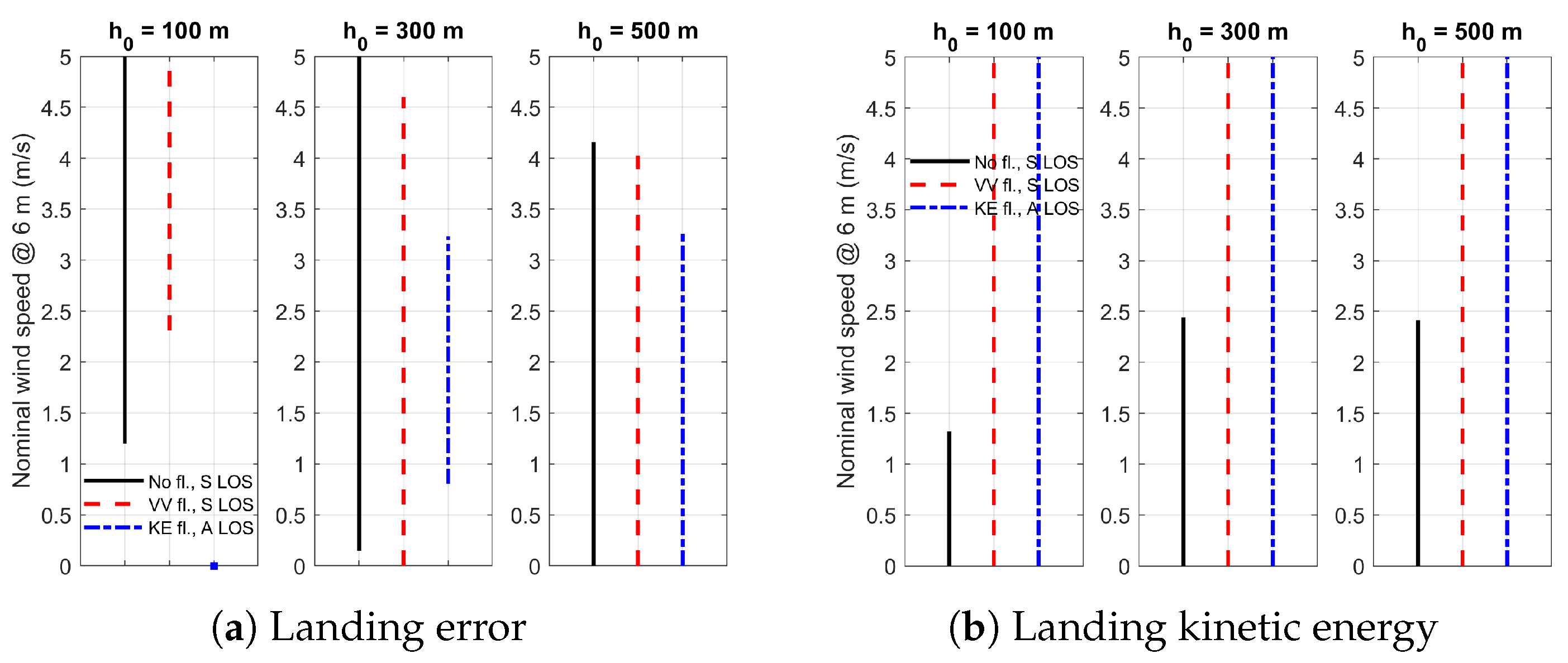
Figure 23.
Performance limits of system with no flare setting and standard LOS guidance, system with kinetic energy reduction flare setting and standard LOS guidance, and system with vertical velocity reduction flare setting and adaptive LOS guidance.
Figure 23.
Performance limits of system with no flare setting and standard LOS guidance, system with kinetic energy reduction flare setting and standard LOS guidance, and system with vertical velocity reduction flare setting and adaptive LOS guidance.
Figure 24.
Performance limits of controllers. The arrows point towards the area in which the controlled system has a lower median landing kinetic energy than the uncontrolled system.
Figure 24.
Performance limits of controllers. The arrows point towards the area in which the controlled system has a lower median landing kinetic energy than the uncontrolled system.
Table 1.
eVTOL mass and inertial properties.
Table 1.
eVTOL mass and inertial properties.
| (kg) | (kgm2) | (kgm2) | (kgm2) |
|---|
| 2100 |
|
|
|
Table 2.
Parafoil canopy mass and dimensions.
Table 2.
Parafoil canopy mass and dimensions.
| (m) | b (m) | c (m) | t (m) | S (m2) | a (m) | (-) |
|---|
| 500 | 23.928 | 9.705 | 1.456 | 232.221 | 3.614 | 2.466 |
Table 3.
Parafoil with eVTOL payload aerodynamic and control derivatives.
Table 3.
Parafoil with eVTOL payload aerodynamic and control derivatives.
| Aerodynamic Derivatives | Control Derivatives |
|---|
|
| 0.25 |
| 0.12/rad2 |
| 0.21 |
| 0.40 |
|
| −0.23/rad |
| 0.091 |
| 2.0/rad |
| 3.95/rad |
|
| 0.90/rad |
| −0.036/rad |
| −0.0035 |
| 0.0015 |
|
| −0.84/(rad/s) |
| −0.08/(rad/s) | | | | |
|
| 0.35 |
| −0.7/rad | | | | |
|
| −1.49/(rad/s) |
| −0.0015/rad | | | | |
|
| 0.082/(rad/s) |
| −0.27/(rad/s) | | | | |
Table 4.
u and w responses of nonlinear and linear systems to step control inputs.
Table 4.
u and w responses of nonlinear and linear systems to step control inputs.
| System | Control Input | (m/s) | (m/s) | Ratio | Ratio % Difference |
|---|
| Nonlinear | (1 unit step) | 4.77 | 3.32 | 0.696 | - |
| | ( step) | 3.73 | 2.9 | 0.777 | - |
| | Combined | 6.21 | 4.99 | 0.804 | - |
| Linear | (1 unit step) | 6.26 | 4.44 | 0.709 | 1.903 |
| | ( step) | 5.23 | 3.83 | 0.732 | 5.809 |
| | Combined | 11.49 | 8.27 | 0.720 | 10.427 |
Table 5.
Parafoil and eVTOL payload system nonlinear model predictive controller parameters.
Table 5.
Parafoil and eVTOL payload system nonlinear model predictive controller parameters.
| Stage Prediction Time () | Prediction Horizon (p) | Number of Stages () | Prediction Time (s) |
|---|
| 0.45 | 2 | 3 | 0.9 |
Table 6.
Parafoil and eVTOL payload system Monte Carlo simulations matrix. “N” represents none, “S” represents standard, “A” represents adaptive, “KE” represents kinetic energy reduction, and “VV” represents vertical velocity reduction.
Table 6.
Parafoil and eVTOL payload system Monte Carlo simulations matrix. “N” represents none, “S” represents standard, “A” represents adaptive, “KE” represents kinetic energy reduction, and “VV” represents vertical velocity reduction.
| ID | Flare Mode | LOS Guidance | Wind Speed at 6 m (m/s) | Initial Heights (m) | Wind Shear | Dryden Wind Turbulence | Parameter Uncertainty | Num. Simulations |
|---|
| 1A | N | S | [0, 1, 2, 3, 4, 5] | [100, 300, 500] | ✓ | ✓ | ✓ |
|
| 1B | N | N | [0, 1, 2, 3, 4, 5] | [100, 300, 500] | ✓ | ✓ | ✓ |
|
| 2A | VV | S | [0, 1, 2, 3, 4, 5] | [100, 300, 500] | ✓ | ✓ | ✓ |
|
| 2B | N | N | [0, 1, 2, 3, 4, 5] | [100, 300, 500] | ✓ | ✓ | ✓ |
|
| 3A | KE | A | [0, 1, 2, 3, 4, 5] | [100, 300, 500] | ✓ | ✓ | ✓ |
|
| 3B | N | N | [0, 1, 2, 3, 4, 5] | [100, 300, 500] | ✓ | ✓ | ✓ |
|
Table 7.
Values of control derivatives for maximum landing error cases of system with vertical velocity reduction flare setting and standard LOS guidance and system with kinetic energy reduction flare setting and adaptive LOS guidance at an initial height of 500 m and nominal wind speed at 6 m of 2 m/s.
| Parameter | Nominal Values | VV Flare,
Standard LOS | KE Flare, Adaptive LOS |
|---|
| Landing error (m) | - | 106.06 | 92.15 |
|
| 0.4 | 0.3827 | 0.3909 |
|
| 0.21 | 0.2116 | 0.2203 |
| (/rad) | 3.95 | 3.8202 | 3.9712 |
| (/rad) | 2 | 2.0752 | 2.105 |
| % variation from nominal ratio | - | 5.05 | 6.84 |
| % variation from nominal ratio | - | 6.79 | 4.48 |
Table 8.
Percentage area of simulation sample space in which the controlled system outperforms the uncontrolled system.
Table 8.
Percentage area of simulation sample space in which the controlled system outperforms the uncontrolled system.
| Control System | Landing Error (%) | Landing Kinetic Energy (%) |
|---|
| No flare, Standard LOS | 88.43 | 43.03 |
| VV flare, Standard LOS | 79.64 | 100 |
| KE flare, Adaptive LOS | 40.73 | 100 |


