1. Introduction
This study provides a comparative analysis of unsupervised machine learning methods to real-world flight data. Flight data monitoring (FDM) is defined in EU law as “a proactive and non-punitive use of digital flight data from routine operations to improve aviation safety conducted by airlines as a means of improving the safety and operation of their aircraft fleet” (Commission Regulation (EU) 965/2012). Modern civil aircraft are required to have flight data recorders with a minimum ability to store 88 flight parameters for 25 h [
1]. The flight data are generally downloaded from the aircraft and analyzed offline through statistical methods to highlight exceedances of flight parameters. Such occurrences of exceedances are then investigated by the airline’s safety officers with the aim of improving safety, through implementing Standard Operating Procedures (SOPs) and promoting good airmanship. However, with progress in data storage technology, aircraft manufacturers have taken the opportunity to record more data, which are then fed into safety reviews for the improvement of their product. For example, the Boeing 787 can record approximately 2000 flight parameters in 50 h. Despite advancements in data recording, the data analysis aspect has been lagging. The traditional analysis techniques can be overwhelming for humans, complicating the detection of patterns in flight data. This may lead experts to focus on obvious issues while missing less apparent dangers. As a result, the proactive potential of the FDM principle may not be realized. Although the introduction of FDM has significantly enhanced aviation safety, it still faces several limitations, specifically the following:
The current occurrence-based system relies on the human operator to establish patterns in exceedances from a particular aircraft or group of flights.
Exceedance occurrences are identified through set thresholds based on past experience, including incidents or accidents. As a result, the system cannot detect internal vulnerabilities or explore unknown safety issues.
As suggested by [
2], redefining incidents and thresholds may mitigate these limitations to some degree, but it will continue to be a drawback of being unable to predict future issues that might lead to incidents. Additionally, the flight safety officer reviews each flight independently, making it challenging to spot trends across the flights. Each flight parameter is assessed individually at every time step, making traditional FDM analysis labor-intensive. Thus, there is a need for a thorough methodology to analyze all fleet data effectively. Machine learning techniques can help uncover these distinctive flight patterns.
Machine Learning Techniques for Flight Data Anomaly Detection
Machine learning (ML) is a subset of artificial intelligence defined as the study that gives computers the ability to learn without being explicitly programmed [
3]. Anomaly detection involves the process of recognizing patterns in data that differ from the anticipated behavior [
4]. A wide range of algorithms and methodologies for the identification of anomalies is available, and a comprehensive literature review has been conducted by [
4,
5]. However, certain techniques are not applicable to flight data because they cannot effectively handle time series data. In recent years, scholars focused on flight safety have introduced methods for anomaly detection aimed at analyzing flight data. A thorough examination of modern methods for analyzing flight data is conducted by [
6].
In a broad sense, anomaly detection methods using machine learning can be classified as supervised or unsupervised, based on flight data processing. Supervised methodologies employ a labeled dataset to facilitate the training of the models. These models, which are trained exclusively on normal data, can recognize anomalous data that they have not encountered before. Conversely, unsupervised methods uncover hidden structures in unlabeled datasets. Unlabeled data refers to information without classification as normal or anomalous. A combination of both unsupervised and supervised methods is referred to as semi-supervised techniques, which typically employ a limited quantity of labeled data alongside a substantial volume of unlabeled data. The process of labeling data is both labor-intensive and costly. It requires the engagement of human experts, which makes it vulnerable to personal biases. Furthermore, datasets that are labeled with anomalies may create an inclination to distort the data as normal data are in high volume as compared to anomalous data. In anomaly detection, the objective is to identify samples that deviate from the normal data pattern. In the application of such methodologies within the aviation sector, the identification or creation of instances based upon particular anomalies is profoundly reliant on human expertise. It is infeasible to obtain all instances of anomalous flights (outliers); consequently, it becomes crucial to choose the appropriate examples for labeling to ensure precise classification with the minimal number of labels. This is known as the problem of label acquisition [
7]. The challenge of anomaly detection discussed in this study cannot be adequately approached through supervised methodologies, as the primary aim is to identify anomalies without any prior knowledge of what constitutes “normal” or “abnormal.” Therefore, unsupervised anomaly detection techniques offer greater benefits in the field of FDM since they assist in discovering the hidden structure or distribution within the data, allowing for a deeper understanding of the data without reliance on labels.
The modern machine learning techniques based on deep learning that demand substantial computational power are beyond the focus of this study. The present study specifically concentrates on traditional unsupervised machine learning techniques and the outcomes achieved through their application to real world flight data. To achieve this, the paper is organized in the following manner:
Section 2 presents a review of the existing literature encompassing unsupervised ML-driven anomaly detection methods put forth for flight data analysis. These techniques are conceptually dissected and compared.
Section 3 introduces real flight data, and the techniques discussed are applied. The results from the various techniques are compared with each other and the current state of the art. In
Section 4, five case studies of anomalous flights are presented, along with the views of the aviation experts. Finally, a discussion and conclusion are presented in
Section 5.
2. Literature Review of Unsupervised Machine Learning Techniques
In the domain of flight data analysis, unsupervised ML methods can be classified as clustering, distance-based, and density-based methods. Although some clustering techniques bear conceptual resemblance to distance and density-based methodologies, the former is optimized to identify clusters, whereas the latter two are primarily oriented towards the identification of outliers. The following subsections highlight how such techniques have been applied to FDM.
2.1. Clustering
Clustering is an unsupervised methodology employed for the clustering of objects possessing common attributes. Each data point contained within a cluster reflects a resemblance to its counterparts within the same cluster. Within a cluster, the data points exhibit similarity, whereas differentiation is upheld among different clusters. Data points that do not belong to any clusters are termed outliers. Depending on the data pre-processing, these datapoints may reflect flight parameters or specific flights in a high or low dimensional space. When employing clustering methodologies on flight data, it is generally assumed that most flights are normal and can be categorized accordingly. As a result, flights that diverge from the predominant flight pattern exhibited by the majority are designated as anomalous. Therefore, this situation necessitates further examination of these anomalous flights to determine the underlying factors that contribute to the anomalous behavior. There exist various methodologies for conducting cluster analysis, including partition-based, proximity-based and hierarchy-based methods.
2.1.1. Partition-Based Clustering
Partitional clustering is the decomposition of a given dataset into a set of joint (overlapping) or disjoint (non-overlapping) clusters. In the case of a dataset containing
N points, a partitioning technique is employed to create
K partitions (where
N is greater than or equal to
K), with each partition serving as a representation of a distinct cluster [
8]. Clustering based on partitioning can be classified into two distinct categories: soft clustering, also referred to as overlapping clustering, and hard clustering, known as exclusive clustering. Soft clustering utilizes fuzzy sets to cluster data, thereby allowing each object to belong to two or more clusters with differing degrees of membership. Conversely, hard clustering arranges objects in a mutually exclusive fashion, signifying that if an object is a member of a specific cluster, it is excluded from membership in any other cluster. K-means is the principal and representative methodology within this category. It segregates the observations into
K clusters with the intention of minimizing the intra-cluster disparity and maximizing the inter-cluster divergence. Each cluster has a mean value called the centroid. Data points are grouped with the closest centroid measured using a metric like Euclidean distance. The goal is to identify
K clusters in the dataset. The user defines the number of clusters as
K, and the algorithm assigns data points to the clusters accordingly.
Figure 1 illustrates the K-means algorithm. K-means is not primarily designed for anomaly detection. Nevertheless, after establishing cluster centroids using this method, a distance threshold can be applied in a subsequent step to pinpoint points that are the most distant from the centroids. A data point is categorized as an outlier when its distance from the cluster’s centroid surpasses the predetermined threshold.
Identifying anomalies through the utilization of partition-based clustering algorithms within the aviation domain was first attempted in 2005 [
9]. Although this work successfully managed to bring attention to flights that deviated from the norm, it had its limitations. In particular, the employment of time series representation to illustrate flight data has been demonstrated to be insufficient in capturing the essential signals inherent within the dataset [
10]. K-means was used in [
11], where a level of membership was assigned to each item in the dataset and then the membership of items was continuously adjusted to solve an objective function. In this work, the K-means and K-medoids algorithms are utilized as hard partitional clustering methodologies, whereas the Fuzzy C-means (FCM) algorithm is implemented as a soft partitional clustering technique. Furthermore, the Fuzzy clustering by Local Approximation of Memberships (FLAME) is additionally employed as a soft partitioning clustering algorithm. K-means relies on the centroid of the cluster, while K-medoid relies on the medoid of the cluster. The findings of this study indicate that as the value of
K increases in the K-medoid algorithm, there is a distinct separation between clusters that are of high quality and those that are of low quality. In addition, the FCM algorithm exhibits a similar clustering pattern to that of the K-means algorithm. On the contrary, the FLAME algorithm exhibits enhanced clarity in the formation of clusters due to its incorporation of a two-step procedure. Initially, the algorithm generates a graph of k-nearest neighbors to detect objects that possess the highest local density, namely objects within the same vicinity. Subsequently, it proceeds to identify objects that exhibit a local density below a specified threshold, thereby classifying them as outliers. Fuzzy memberships are assigned exclusively to objects in regions of highest local density, and not to objects in regions of lower local density. The primary limitation of partition-based clustering algorithms is the necessity to determine the number of clusters in advance. If the cluster count is not suitably established, the resulting clustering configuration may be ambiguous in its definition.
2.1.2. Proximity-Based Clustering
The proximity-based approaches identify clusters by assessing how close a specific point is to its surrounding points, assuming that points included within a cluster are in close range to each other and have similar proximity to their individual neighbors. It is essential to establish a defined distance function to quantify this proximity. Density-Based Spatial Clustering of Applications with Noise (DBSCAN) [
12] is the prominent clustering algorithm that functions based on the principle of proximity. It has been used a lot to detect anomalies in the flight data. DBSCAN partitions the data points by creating a circle with a radius of
ε (epsilon) around each point and then classifies them into three separate categories: core points, border points, and noise. A data point is recognized as a core point if the circle that surrounds it contains at least a specified number of points known as
minPts. On the other hand, if the point count is below the
minPts threshold, it is classified as a border point. If there are no additional data points located within the
ε radius around a particular data point, it is deemed to be noise. Clusters are formed automatically until all the data points have undergone processing. This approach does not necessitate any pre-existing knowledge regarding the number of clusters present in the dataset.
Figure 2 demonstrates the working of the DBSCAN algorithm.
In
Figure 2, all data points that contain at least three points, including themselves, within a circle of radius
ε are referred to as core points, represented visually by the color blue. Data points that have fewer than three but more than one point, including themselves, within the circle are categorized as border points, depicted in orange. Finally, data points that lack any other points, apart from themselves, within the circle are recognized as noise, indicated by the color red. DBSCAN is traditionally crafted to group similar data points. However, in the realm of anomaly detection, those data points that would usually be categorized as noise (i.e., the byproduct of clustering) transform into outliers. The DBSCAN algorithm has been utilized in various studies [
10,
13,
14] to identify outliers within flight data. In [
10], an anomaly detection approach was developed based on DBSCAN, making it one of the research pillars in the history of FDM. The author has developed two algorithms, namely Cluster Anomaly Detection (CAD)-Flight and CAD-Data Sample. CAD-Flight uses DBSCAN and the CAD-Data Sample clusters datapoints using a Gaussian Mixture Model (GMM). GMM is a combination of the statistical approach, classification approach (supervised learning) and clustering approach. A GMM is a parametric probability density function represented as a weighted sum of Gaussian component densities [
15,
16,
17]. When it is used for anomaly detection in CAD-Data Sample, a mixture of Gaussian components for normal data is developed. Each component is a multivariate Gaussian distribution that signifies a type of normal data. The test data are classified as anomalies if they do not pertain to any of the Gaussian components. The fundamental distinction between these two clustering techniques resided in the employed algorithm and the way every flight was handled. For analysis, CAD-Flight considers each flight within a fleet as an individual vector in a multi-dimensional space, known as hyperspace. Conversely, CAD-Data Sample treats each flight parameter acquired from the sensor as an independent vector. Remarkably, both algorithms have demonstrated the capability to identify operationally significant anomalies that surpass existing methods. However, these algorithms exhibit deficiencies in recognizing local outliers (outliers local to a cluster) and are solely capable of detecting global outliers (outliers common to all the clusters) since they do not take into account the density of a neighborhood when assessing outliers.
2.1.3. Hierarchical Clustering
A hierarchical clustering method generates a series of divided data points. It gradually merges smaller clusters into more significant ones or splits larger clusters apart. In both methods, two key metrics are necessary to determine whether the clusters should be merged or separated. The two key metrices are as follows: a measure that quantifies the distance between observations when considered in pairs, and a criterion that defines the degree of dissimilarity among the clusters. The outcome of the algorithm is a cluster hierarchy, showcasing the relationships between the clusters [
18]. BIRCH [
19] and CURE [
20] are two examples of algorithms that utilize a hierarchical approach to cluster large datasets. The HDBSCAN [
21] clustering algorithm was used in [
22] to classify flights as normal or anomalous. The algorithm expands upon DBSCAN through the process of transforming it into a hierarchical clustering technique, subsequently employing a method for extracting a flat clustering that is predicated on the stability of clusters. The HDBSCAN algorithm provides the capability to identify and label specific data points as noise, thereby avoiding the need to assign these samples to a particular cluster. Most of these noisy samples tend to be situated in proximity to the boundary between two distinct groups, or they may be located sufficiently far away from any identified cluster.
Despite being the preferred method for identifying anomalies in flight data, clustering possesses a fundamental drawback. Clustering techniques such as DBSCAN, BIRCH, and CURE have the capability to identify anomalous data points. Nevertheless, the primary goal of clustering methods is to identify clusters of similar data points and thus, their development is focused on optimizing clustering rather than optimizing the detection of anomalies. The interpretation of an outlier is contingent upon the clusters that are detected by these algorithms. Henceforth, certain methodologies were devised with the sole intention of identifying anomalies. Outliers are detected in an optimized manner, rather than being a consequence of clustering. The identification of outliers in these methods can be density based or distance based.
2.2. Distance-Based Methods
Distance-based methodologies characterize outliers as observations that are situated at a specified minimum distance from a particular percentage of the observations within the dataset. In distance-based methods, outliers are the points usually farthest away from other points. One major difference between distance-based approaches and the other two categories is the degree of detail at which the analysis is conducted. In both clustering and density-based approaches, the data are first grouped before outlier analysis by either dividing the points or the dimensional space. The data points are then compared to the distributions in this pre-grouped data for analysis. On the contrary, in distance-based methods, the outlier score is computed as the k-nearest neighbor distance to the original data points (or a similar variant). Hence, the analysis in nearest neighbor methods is conducted at a more complex level compared to clustering methods [
23]. Ref. [
24] proposed a distance-based outlier detection technique based on the idea of nearest neighbors and is the most popular method in this category. The research conducted by [
25] utilizes iOrca [
26], an indexed version of the Orca [
27] algorithm created to analyze genuine datasets from a commercial airline during the descent phase of a flight. Orca, an unsupervised anomaly detection algorithm that relies on the k-nearest neighbor approach, employs a nested loop structure to compute the distance between individual data points. In the study conducted by [
26], a pioneering approach to indexing and an early termination criterion were introduced by the authors to enhance the scalability of Orca for exceedingly large datasets. However, the distance-based methods tend to become complex since every data point needs to be compared to every other, to find the distance between the two points or two flights in case of flight data.
2.3. Density-Based Methods
Density-based techniques employ the count of data points (flights) in particular areas of space to define anomalies. Density-based methods detect outliers as objects that are in a less-dense region in high dimensional space than the rest of the dataset. Generally, objects are outliers relative to their neighborhoods when density of their neighborhoods is considered. These methods require distance function to quantify the density of the neighborhood. They have a strong connection to clustering and distance-based techniques. In fact, depending on their presentation, some of these algorithms can be more readily viewed as clustering or distance-based techniques. This is due to the close relationship and interdependence between the concepts of distances, clustering, and density. Numerous algorithms in this category can uncover outliers that are sensitive to locality. Locality refers to the local environment using the k-nearest neighbor (kNN) algorithm and the density of this local environment or neighborhood is termed as local density. This study centers its attention on one such methodology called Local Outlier Factor (LOF) by examining its theoretical advantages, as well as evaluating the outcomes on a dataset. The algorithm assigns an outlier score to every data point, referred as LOF [
28], which is computed by comparing the local density of an object with the local densities of its neighboring points. Data points that exhibit significantly lower density than their neighboring points are deemed as outliers. The development of Local Outlier Probability (LoOP) [
29] aimed to address the challenge of interpreting the numeric outlier score from LOF when determining if a data object is truly an outlier. LoOP is less dependent on parameter k of the k-nearest neighbor (kNN) in the LOF algorithm. By utilizing the LoOP technique, an outlier score between 0 and 1 is provided, allowing for direct interpretation as the probability of a data object being an outlier. Ref. [
30] uses LoOP to detect anomalies in flight data. This contrasts with the application of LOF in this study in terms of the processing of raw data and the manner in which flight data are integrated into the algorithm. In [
31], a statistical model is employed alongside LOF to identify anomalies in flight data. The application of LOF in the method presented in this study differs from this study, concerning the determination of the optimal
k parameter, data preprocessing, and the subsequent adjustment of the threshold value. While methods utilizing the Local Outlier Factor (LOF) have been used previously to detect anomalies in flight data, they were implemented differently during both the pre-processing and processing stages of the flight data. In addition to pre-processing and processing stage, this study introduces the application of LOF in a hybrid manner, wherein LOF is utilized alongside a statistical method for the post-processing of flight data. In the study conducted by [
22], they propose a novel approach by combining the HDBSCAN clustering algorithm with the Global-Local Outlier Score from Hierarchies (GLOSH) algorithm. The combination aims to address a common drawback of clustering algorithms, which is their tendency to overlook local outliers. Other techniques within this particular category include the Local Correlation Integral (LOCI), methods based on Histograms, estimations using Kernel Density, and approaches utilizing Ensembles.
Jasra et al. [
32] discussed a method to decide the optimal value of parameter
k in case of flight data analysis while using LOF. In this work, the LOF method is employed alongside Tukey’s method, a statistical technique, to identify flights that exhibit anomalous behavior, unsafe practices, or procedures that deviate from SOPs. Hence, the integration of machine learning (ML) with a statistical method results in a hybrid approach that effectively detects anomalous flights with the least possible occurrence of false positives. The hybrid approach exhibits sufficient robustness in order to diminish the quantity of false alarms, which may arise from automated anomaly detection methodologies. Consequently, this mitigates the constant dependency on a human specialist to determine the legitimacy of an outlier’s anomalous nature.
Figure 3 illustrates the step-by-step implementation of the hybrid LOF method. The robust threshold value employed in this hybrid LOF approach limits the definition of an anomalous flight, and this value is determined dynamically based on several factors, including the set of flights provided as input and the specific airport being analyzed. This value is specific to each airport and becomes more consistent as the number of flights increases as shown in the work [
32]. It has been demonstrated that the degree of anomalous behavior can be measured using the hybrid method, which assigns a score to each flight. A score of 1 or less than 1 indicates a theoretically normal flight, while a score surpassing the statistically determined threshold signifies a truly anomalous flight. This score compares the severity of the anomaly among multiple anomalous flights.
The hybrid LOF approach detects the specific time frame during the flight when the flight itself was anomalous, thus monitoring anomalous behavior over time. It is valuable when a flight deviates from the norm for a brief period, as it also allows us to identify the corrective actions taken to rectify the anomaly. Additionally, this approach highlights the flight parameters that contribute to anomalous behavior. Thus, the key advantages of LOF over other methods include anomaly score assigned to a flight, the extent of abnormality of an anomalous flight is measured throughout the timeline, and the parameters responsible for the anomaly are determined. The research undertaken by [
33,
34,
35] has demonstrated the superiority of LOF which is the base for hybrid LOF approach in comparison to clustering and various other anomaly detection techniques. Ref. [
36] demonstrated the effectiveness of the LOF methodology in identifying novel patterns within the datasets derived from ventilation and water pumping systems in the context of the Industrial Internet of Things. Ref. [
34] elucidated that the LOF method exhibited superior performance relative to alternative techniques when attempting to detect novel incidents of network intrusion. The characteristics of network attacks consist of infrequent anomalies amidst a large volume of regular data, which is similar to safety incidents found in FDM data. Ref. [
37] conducted an examination of diverse methodologies for outlier detection, ultimately concluding that the traditional Local Outlier Factor (LOF) technique continues to be considered one of the most advanced approaches.
3. A Comparison of Real-World Applications of ML Techniques
This section applies K-means, DBSCAN and hybrid LOF to a real-world flight dataset. The subsequent subsections provide a detailed explanation of the procedures involved in implementing each technique, emphasizing the significant distinctions in the execution of each method.
3.1. Flight Dataset
Real-world flight data are not easily accessible due to the sensitivity nature of airline operations and pilot personal data protection. In 2012, the National Aeronautics and Space Administration (NASA) released an extensive database of multivariate time series flight data in the public domain [
38]. The database, totaling 250 GB, relates to approximately 170,000 flights that took place between 2001–2003 and 2010. A total of 35 tail numbers have been documented as they navigate between 90 airports located throughout the United States of America. Each flight captures 186 unique flight parameters, with sampling frequencies varying from 1 Hz to 16 Hz. To safeguard the identities of the airlines and the flight crew, the flight data have been properly de-identified by NASA.
3.2. Data Pre-Processing
The data, which were stored in MAT files, underwent a transformation process in order to be represented in the format of Structured Query Language (SQL) tables. This conversion facilitated the efficient retrieval and utilization of the data for ML algorithms. For each individual flight, a set of 132 flight parameters, deemed to be crucial by the experts in the industry, were taken into consideration. The deliberate exclusion of dynamic weather parameters ensures that all flights are treated uniformly and are not impacted by environmental factors. Any weather-related occurrence that affects the behavior of the crew will be documented using other flight indicators. Certain flight indicators that have fixed values, such as engine number, were also eliminated from the analysis. The values of all 132 flight indicators were standardized because each flight parameter had a distinct range of values and units. The dataset was thoroughly examined to identify and rectify any missing values or disturbances. These flight parameters were sampled at rates ranging from 1 hertz to 16 hertz. In order to align the data points, all flight parameters were converted to a sampling rate of 16 Hertz by interpolating the values of parameters sampled at lower rates. For analysis, the final three minutes of flight duration, which includes the approach and landing stages, are considered. The precise location where each aircraft made contact with the ground was determined by taking into account various flight parameters, including the phase of the flight (PH), the presence of weight on the wheels (WOW), as well as the latitude (LAT) and longitude (LONG) coordinates. The latitude (LAT) and longitude (LONG) coordinates were utilized to pinpoint the exact runway that was used. Furthermore, all the flights were adjusted to the specific altitude of the airport, thus eliminating any negative values for the flight parameter altitude. Consequently, by working through the flight timeline in reverse, it was possible to align all the landings of the aircraft on the same runway in a perfect manner, synchronizing them in terms of the time at which touchdown occurred.
Figure 4 depicts a plot that illustrates the relationship between the flight parameter of altitude (ALT) and time, based on data from 674 flights originating from a single tail number (652) and arriving at Detroit Airport, following the completion of all necessary data pre-processing.
This methodology stands in stark contrast to earlier studies [
11,
13,
14,
30,
39,
40] wherein altitude and the distance to touchdown serve as the evaluative parameters for the consideration of flight timeline. The rationale for the consideration of such a timeline is based upon the fact that Standard Operating Procedures (SOPs) utilized during the approach and landing phases are predominantly specific to either altitude or distance, rather than being contingent upon time.
Figure 5 illustrates the methodology employed by [
13], where every flight under 50 feet in altitude was taken into account for analysis of flight data.
In similar studies, the altitude is plotted against the distance (nautical miles) to touchdown. The primary constraint of such methodologies lies in the fact that each flight will exhibit a differing number of timesteps, as not all flights will be positioned at the same distance to landing at a specific altitude or at an equivalent altitude with identical time remaining before descent. For example, one flight may descend below 50 feet 10 s prior to landing, while another may do so 6 s before landing. Clustering and the LOF algorithm necessitate having an identical number of time steps. Consequently, examining the final three minutes of each flight prior to touchdown, as established in this study, ensures a uniform count of time steps. Methodologies based on altitude and distance require interpolation to incorporate the values of flight parameters for flights with shorter duration, as performed by [
13]. This process poses a risk of distorting essential information. The timing is crucial during the last phases of flight as the crew needs extra time to react to an event. Analyzing flights by their remaining time to touchdown helps understand crew behavior and identify anomalies in the dimension of time.
3.3. Selecting Approach and Landing Phase as a Case Study
In order to place boundaries around this comparative analysis, investigation was limited to the approach and landing portions of the flight as it is the most critical phase of a flight. In the past twenty years, more than half of all fatal and non-fatal incidents resulting in the loss of the hull of an aircraft occurred during the phase of approach and landing, despite the fact that this particular phase only accounts for approximately four percent of the total duration of the flight [
41,
42]. Consequently, for the purpose of analysis, the final three minutes of flight duration, which includes the approach and landing stages, are considered. Many flights tend to become unstable during this phase. Traditionally, a stable approach is defined by a set of rules as summarized in
Table 1. When aircraft data demonstrate that at least one of these rules was not respected (through an exceedance in the flight parameter data), the approach is considered unstable, and the flight is investigated. The comparative analysis was conducted on a single tail number (Tail 652) encompassing a total of 674 flights landing at Detroit Metropolitan Wayne County Airport (DTW) in the United States of America.
3.4. A Comparison Between K-Means, DBSCAN, LOF and Hybrid LOF
In this examination, a total of 674 flights from a single tail and landing at Detroit International Airport (DTW) were carefully analyzed for any anomalous activities. During the implementation of the K-means clustering, the number of clusters was chosen as two using the elbow method. The elbow method serves as a heuristic for identifying the optimal number of clusters within a dataset. This approach involves graphing the explained variation in relation to the number of clusters and selecting the point where the curve bends, known as the elbow, to determine the appropriate number of clusters to utilize. The Silhouette method [
43] also confirmed this value. The threshold distance was established at 12.5, as there were no additional anomalies beyond this point.
K-means methodology detected 10 anomalies, as illustrated in
Figure 6, which predominantly consisted of long-term anomalies, including un-stabilized approaches that persisted until touchdown.
DBSCAN (
ε = 0.11825,
minPts = 11), conversely, detected 55 anomalous flights, as illustrated in
Figure 7, which is much more as compared to the findings of the K-means clustering. The optimal ε was established using Dynamic Method DBSCAN (DMDBSCAN) articulated by [
44].
In the execution of the LOF methodology, a
k value of 33 was chosen, as detailed in method discussed in [
32]. The threshold was defined at a LOF score of 1 following the guidelines provided in the foundational study of LOF [
28]. As a result, a total of 115 flights were identified as anomalous, as depicted in
Figure 8. During the process of verification and validation by aviation experts, it was noted that, from an industry viewpoint, numerous flights classified as anomalous by the LOF technique were, in reality, regarded as standard.
The theoretical threshold of 1 for the LOF value led to a substantial rise in the number of false positives. An initiative was undertaken to modify the threshold through collaborative discussions with experts, analyzing each flight individually. Different values were employed to fine-tune the threshold. Nonetheless, it became clear that a more systematic methodology is essential to accurately adjust the LOF threshold, aiming to reduce false positives and strengthen the process’s reliability, thereby decreasing its dependence on human input. The literature review also highlighted a research gap in the fine adjustment of the threshold to effectively eliminate false positives for anomalies detected in flight data. There exists no established benchmark to determine a threshold for distinguishing false positives from true anomalies. Consequently, hybrid LOF was utilized on the outcomes derived from the LOF method (k = 33) to limit the number of false positives. The newly established dynamic threshold value was determined through the application of Tukey’s method on the LOF score of all flights, with the objective of mitigating false positives. The LOF value of 1.4005 was established as the new threshold in contrast to the default threshold value of 1. Consequently, 26 flights have been classified as anomalous, a significant reduction from the previous count of 115 flights as shown in
Figure 8. Thus, the 89 flights that were formerly categorized as anomalous, were reclassified as normal through the implementation of a hybrid LOF threshold.
Figure 8 shows the LOF score of all flights arriving at DTW and the new hybrid threshold value compared with the default LOF threshold value.
The terms ‘anomalous flights’ or ‘abnormal flights’ defined by this approach means flights with unusual data patterns. This is not the same as ‘unsafe flights’ or ‘risky flights.’ Flights with unusual data patterns are of interest for detection, but they need further investigation by human experts to determine whether they represent any safety risks. These results were then verified against the traditional rule-based approach and validated by the industry experts. The validation process is described in the next section.
4. Validation and Comparison of Results
A total of 115 flights that were originally identified as anomalous using the LOF methodology were selected for validation. This selection encompassed the entire collection of anomalous flights recognized by every method employed. The validation of these flights will facilitate the identification of both false positives and false negatives associated with each respective method. For all 115 of these flights, industry experts examined data from the five minutes prior to landing, which included all 132 flight parameters. The experts began their investigation with 26 out of the 115 flights that had been identified as anomalous by the hybrid LOF method. It was established that 25 out of the 26 anomalies were correctly identified by hybrid LOF. The flights exhibited anomalies primarily due to unstable approaches (high-energy approaches) and a delayed landing configuration of the aircraft. Certain flights displayed anomalies attributed to weather factors, engineering issues, and operational challenges. However, one flight that was labeled as anomalous by the hybrid LOF because of its unusually brief approach conformed to aviation standards. Consequently, this was considered a false positive by hybrid LOF. The flight’s brief duration could have been influenced by directives from Air Traffic Control (ATC) or adverse weather conditions. The other methods accurately identified it as normal. Subsequently, the remaining 89 flights with LOF scores above 1 were scrutinized to identify any instances of false negatives, as these flights had been designated as normal by the hybrid technique. Initially, the top 20 flights with the highest LOF scores were selected from this group of 89 flights. Each individual flight was reviewed to determine its anomalous nature. None of these 20 flights were determined to be false negatives. As the remaining 69 flights exhibited even lower LOF scores, they were also presumed to be within the normal range. Thus, this validation procedure categorized 115 flights into 25 legitimate anomalies and 90 legitimate normal flights. This categorization served as the ground truth for the evaluation of each technique.
Figure 9 presents a qualitative analysis comparing the traditional approach with various unsupervised machine learning techniques in relation to the ground truth. In this figure, flights identified as anomalous by each technique are depicted in distinct colors, while the white areas in between represent flights categorized as normal by the respective technique. The x-axis illustrates the total of 115 flights. The y-axis enumerates all the techniques being compared. Beginning with the verification by domain experts, only 25 out of the 115 flights were identified as genuine anomalies. These anomalies are highlighted in green. The white areas in between represent flights that were deemed normal. Secondly, 22 flights, indicated in brown, were accurately classified as anomalous by the traditional method. Nonetheless, the traditional approach failed to identify 3 anomalous flights that were outside the specified parameters or boundaries outlined in
Table 1. Thirdly, K-means accurately identified 10 flights in purple as anomalous. In total, it overlooked 15 anomalies. Additionally, DBSCAN detected 55 anomalies represented in orange. Out of these, only 21 were consistent with the ground truth. Consequently, it failed to recognize 4 legitimate anomalies and identified 34 false positives. Lastly, hybrid LOF recognized 26 anomalies displayed in red. Among these, 25 were consistent with the ground truth, while one was categorized as a false positive mentioned previously.
In order to obtain a deeper insight into the results and verify the correctness of each technique, a quantitative analysis employing a confusion matrix was performed. A confusion matrix facilitates the evaluation of the results from each specific technique against the ground truth. It consists of a 4 × 4 based on true positives, false negatives, false positives, and true negatives.
Figure 10 illustrates the confusion matrix corresponding to each technique being examined.
The traditional rule-based method overlooks three instances of anomalous flights, as illustrated in the confusion matrix. These instances are classified as false negatives. Nevertheless, it accurately detects 34 instances of normal flights. Therefore, it has a precision rate (PR) of 1 and a recall rate (RR) of 0.88.
The precision rate is the ratio of the number of true positive instances to the sum of true positive and false positive instances as shown in Equation (1).
This criterion indicates how many of the anomalous flights were correctly labeled by the technique. The PR is employed to measure the occurrence of false positives, where a normal flight is mistakenly identified as anomalous.
Conversely, the recall rate is the ratio of the number of true positive instances to the sum of true positive and false negative instances, as shown in Equation (2).
This criterion indicates how many anomalous flights were actually captured by the technique. The RR is used to measure false negatives, where an anomalous flight is incorrectly classified as normal.
In order to achieve a combined effect of false positives and false negatives, the F-1 score is used to achieve the combined accuracy. The F-1 score is the harmonic mean of precision and recall. The harmonic mean is preferred over the arithmetic mean because it is better suited for combining ratios with different denominators. The harmonic mean is defined as:
The traditional method achieves a F-1 score of 0.94. The same process was repeated for all techniques and shown in
Table 2. It can be seen that the hybrid LOF technique achieves the highest overall F-1 score of 0.98. This is closely followed by the traditional rule-based method with an F-1 score of 0.94. Both K-means and DBSCAN score poorly in the F-1 score with 0.57 and 0.53, respectively. This is largely due to their inability to detect local outliers and their lack of ability to fine-tune the technique and eliminate false positives.
5. A Review of Case Studies
Having compared the various techniques, this section presents five cases of validated anomalous flights that have been identified through the hybrid LOF technique implemented for various tail numbers and airports. Each case study delves deep into the specifics of the flight, the time frame during which the abnormal behavior occurred, and a comprehensive analysis of the flight parameters that contributed to the anomaly.
Figure 11 depicts the geographical representation of these case studies.
5.1. Case 1
The flight departed from Blue Grass Airport in Lexington, Kentucky, United States at 09:54 GMT for Detroit International Airport in Romulus, Michigan, United States on 7 November 2002. This flight was flagged anomalous due to potential issues with engine number three and the unusual use of air brakes. The flight parameters contributing to anomalous behavior highlighted were mainly related to engine number three and the intermittent use of air brake and are listed below:
The data for the last three minutes leading up to the landing, encompassing all engines of this anomalous flight, were plotted. As illustrated in
Figure 12, the data points corresponding to engine fan speed (N1) and core speed (N2) of engine number three exhibit a significant deviation compared to those typically observed in the majority of normal flights under investigation.
Figure 13 presents a comparative analysis of the engine fan speed (N1) and core speed (N2) pertaining to engine number three of the anomalous flight in relation to the other flights under scrutiny. The green solid line positioned centrally signifies the median value of this flight parameter, whereas the red dotted line illustrates the values corresponding to this anomalous flight. The blue shaded region shows the statistical distribution for flight parameters.
The utilization of the air brake was significantly high compared to other flights in order to decelerate the aircraft within a time frame spanning from 120 s to 80 s prior to the touchdown, as illustrated in
Figure 14 (left); 120 degrees refers to when the air brake is not being used. The altitude depiction provided in
Figure 14 (right) indicates that throughout this interval, the aircraft, following a “hot and high” approach, successfully decelerated and confirmed to the normal profile upon activation of the brake. Both the utilization of the air brake and the values pertaining to the altitude profile exhibit a notable level of anomaly when compared with the rest of the flights. The values for both these parameters fall out significantly from the statistical distribution measure. The anomaly score plot presented in
Figure 15 illustrates the anomalous behavior of this particular flight during the duration of the analysis. The hybrid LOF methodology facilitates a comprehensive understanding of the dynamics of any flight at any specified timestep throughout the flight’s entirety. This stands in contrast to the prevailing state of the art or other research-oriented methodologies, wherein the analysis is not conducted at each individual timestep but rather over the entire flight duration, aggregating all timesteps collectively. It is evident that the anomaly score peaks between 120 s and 80 s before touchdown, coinciding with the high utilization of the air brake. Moreover, the anomaly score remained elevated during the initial 60 s when the altitude profile displayed a steep decline. The anomaly score reaches its peak around the 60 s mark, corresponding to the moment when the engines commenced rotation after a period of idleness, a behavior not observed in normal flights.
Upon examination by human experts, it was found that the flight utilized air brakes excessively to decelerate the aircraft, a behavior in line with the crew’s efforts to stabilize the aircraft and configure it for landing. While the crew could have chosen to extend the landing gear early to reduce speed, it is possible that their focus was on addressing the issue with engine number three, leading to the predominant use of air brakes for deceleration. It is noteworthy in this instance that engine number three displays a delay in throttle response, warranting a thorough inspection. In such situations, the engine can be dispatched for maintenance instead of waiting for the necessary number of hours to elapse before the maintenance is performed. Timely detection of such occurrences aids in lowering insurance and maintenance expenses. The current state-of-the-art FDM may not detect this issue, highlighting the added benefit of the algorithm in enabling proactive maintenance to prevent further complications.
5.2. Case 2
The flight departed from Nashville International Airport in Tennessee, United States at 10:38 GMT for Minneapolis–Saint Paul International Airport in Minnesota, United States on 6 November 2002. This flight was identified as anomalous due to potential concerns regarding the functionality of engine number three. It is significant to note that this specific aircraft is the identical one previously examined in the initial case. The issue pertaining to engine number three was consequently present beforehand and remained unaddressed. The same aircraft continued its flight from Nashville to Minneapolis and thereafter from Minneapolis to Lexington. Ultimately, it proceeded to fly from Lexington to Detroit the following day, as documented in case one. This case highlights that while traditional flight data monitoring (FDM) systems failed to detect the anomaly, the machine learning (ML)-based algorithm consistently identified the issue involving a delay in throttle response for engine number three. In the last three minutes of approach and landing into Minneapolis-Saint Paul international airport, the algorithm has once again pinpointed flight parameters associated with anomalous behavior, primarily linked to engine number three, which are listed below:
[PLA_3]: Powe Lever Angle for Engine Number 3;
[N2_3]: Engine Number 3 Core Speed (N2);
[N1_3]: Engine Number 3 Fan Speed (N1).
Figure 16 shows that the Power Lever Angle for engine three was idle for the last three minutes of flight duration.
Figure 17 further illustrates that the values of engine number three fan speed and core speed are not in sync with other engines. Unlike the previous case, here the crew skillfully managed to maintain the aircraft within the typical flight profile as none other parameters were highlighted as anomalous. There is a possibility that the complications associated with engine number three deteriorated, consequently affecting additional flight parameters on the subsequent day as detailed in case 1.
5.3. Case 3
The flight departed from Cincinnati Northern Kentucky International airport, Cincinnati, United States at 17:02 GMT for Detroit International Airport in Romulus, Michigan, United States on 18 January 2001. This flight was deemed anomalous as a result of the approach not being stabilized. The flight parameters contributing to anomalous behavior highlighted were as follows:
[LGDN]: Landing Gear Down;
[FLAP]: Flap Setting Values;
[IVV]: Initial Vertical Velocity;
[GS]: Ground Speed;
[ABRK]: Air Brake;
[N1_1 to N1_4]: All Engines’ Fan Speed (N1) values;
[PLA_1 to PLA_4]: All Power Lever Angle values.
Flight parameters LGDN and FLAP corroborate an un-stabilized approach.
Figure 18 shows that the landing gear was deployed only 60 s before the touchdown and the flaps were fully configured less than 40 s before touchdown. By comparing flap settings in
Figure 18 (right) and the altitude profile in
Figure 19 (left), it could be noted that the flight crew was attempting to follow the glideslope between 2500 feet and 500 feet. However, they went lower the normal profile, and the aircraft descended below 500 feet Above Aerodrome Level (AAL) approximately 50 s before landing, still lacking full configuration for a stable approach.
Figure 19 (right) illustrates the air brake (ABRK) of this anomalous flight over time, revealing that the air brake was never engaged and thus not allowing the aircraft to slow down. A faulty air brake could have been the primary cause for the un-stabilized approach.
Figure 20 illustrates the anomaly score of this anomalous flight. Throughout the final three minutes prior to landing, the anomaly score remains notably elevated. The anomaly score peaks at approximately 100 s before touchdown, coinciding with the delayed initiation of flap configuration by the aircraft as depicted in
Figure 18 (left). The anomaly score reaches its highest point near the touchdown point, suggesting a departure from normalcy in the aircraft’s operation, consistent with various flight parameters indicating an unstable approach.
Figure 21 (left) indicates a significant descent rate observed between 80 and 40 s prior to touchdown by this anomalous flight. The Inertial Vertical Velocity (IVV) recorded a value of 1400 feet per minute during this period, which is almost double the suggested value of 750 feet per minute. This anomaly could also be corroborated with the change in gradient of descent in
Figure 19 (left) between 60 and 40 s.
Figure 21 (right) depicts the Ground Speed (GS) of this anomalous flight in relation to the time until touchdown. It is apparent that, in the case of this specific flight, the Ground Speed did not stabilize and consistently decreased until landing.
Figure 22 and
Figure 23 depict the status of each of the four engines’ fan speeds (N1) and the angles of all power levers, in that order, during this unusual flight. It is evident from these illustrations that the engines remained idle until the aircraft made contact with the ground. Consequently, thrust was never established for a stabilized approach. Since the aircraft had excessive speed, the aircraft glided down towards its destination. Such high energy descents are often a risk for runway excursions.
When reviewed by human experts, it was concluded that the flight exhibited a significantly destabilized approach, with all landing related parameters showing anomalous values. The un-stabilized approach is the primary factor contributing to the consistently high anomaly score observed throughout the flight analysis, peaking during the touchdown. The attainment of a stabilized approach is imperative for the safe and effective landing of an aircraft, a criterion that this particular flight failed to meet. Such instances pose a heightened risk level. In accordance with Visual Flight Rules (VFRs), during the early 2000s, it was necessary for aircraft to be established in a stable approach prior to descending to 500 feet, a standard that this flight failed to meet. A preliminary investigation indicated that meteorological conditions did not play a role in the approach path. Nonetheless, further investigation is essential, involving key stakeholders such as Air Traffic Control (ATC) and the flight crew.
5.4. Case 4
The flight departed from Birmingham International Airport in Birmingham, Alabama, at 15:44 GMT for Detroit International Airport in Romulus, Michigan, United States on 22 April 2001. The flight parameters that contribute to anomalous behavior have been identified as the following:
The Localizer (LOC) offers azimuth guidance, whereas the glideslope (GLS) establishes an accurate vertical descent profile. The heading of an aircraft may vary from its track because of the influence of the wind. The variation in aircraft heading is formally referred to as the drift angle and is depicted in
Figure 24.
Figure 25 (left) showcases the data reflecting the Localizer Deviation (LOC) of this anomalous flight over time until it landed. A notable and sudden shift in LOC values is evident between 140 and 80 s before touchdown when compared to the typical pattern. Within just a few seconds, the LOC measurement for this flight escalated from 0.02 Difference in the Depth of Modulation (DDM) to 0.36 DDM. Following this, the flight crew required almost 60 s to correct this deviation while closely monitoring the movement of the LOC indicator towards the right.
Figure 25 (right) is employed to demonstrate the comparison between the drift angle (DA) values of the anomalous flight and the standard pattern, to reinforce the LOC deviation. The DA value recorded during the anomalous flight corresponds with the LOC values pertinent to this flight anomaly. In the absence of any corrective actions, the aircraft drifted to the left, leading to the LOC indicator bar shifting towards the right.
When reviewed by human experts, it was found that this deviation in LOC first and then DA was due to a weather-related event. When reviewing the weather data for the same time window, the Wind Direction (WD) underwent a rapid shift from 20 degrees to 65 degrees to the right within approximately 30 s (160 s to 130 s), occurring during a crucial time in the landing process. The values plotted in
Figure 26 (left) illustrate this abrupt WD shift (highlighted by small red circles) and compare the WD of this anomalous flight with the median of values observed in other normal flights. During the reviewing process peak Wind Speed (WS) of 17 knots was observed at the maximum deviation point for this anomalous flight further supporting the deviation due to big changes in direction and speed during this last phase of the approach to landing.
Figure 26 (right) plots parameter True Heading, which indicates where the aircraft’s nose is pointing relative to True North. A big shift can be seen after the wind gust which corroborates that this was caused by the sudden increase in wind speed and direction. Due to the wind gusts impacting the aircraft at a pivotal moment during the landing procedure, the crew might have become momentarily distracted while trying to adjust for this occurrence. Nevertheless, the landing gear and flaps were subsequently engaged later than intended, as illustrated in
Figure 27. Consequently, these flight parameters suggest an unusual incident stemming from the crew’s delayed response to a weather-related situation; however, this irregularity was ultimately managed safely, and the aircraft remained under secure control until it touched down. This flight also emphasizes the significance of factors beyond human influence and the time taken to respond in order to lessen the impact of such occurrences.
5.5. Case 5
The flight departed from Bishop International Airport in Flint, Michigan, United States at 10:06 GMT for Detroit International Airport in Romulus, MI, United States on 21 October 2002. The flight parameters that were identified as contributing to anomalous behavior were primarily associated with the landing and approach phase. The following are the parameters in question:
The flight in question adhered to standard aviation procedures. However, upon closer examination, it was revealed that the aircraft followed a different flight path while landing compared to other flights traveling between the same departure and arrival airports. The deviation in flight path can be observed in
Figure 28, where the majority of flights approach the runway from a different direction than that of this particular flight.
Aviation experts concluded that this procedure is a standard occurrence caused by weather conditions or issues related to air traffic. The experts have hence classified this as a false positive. Despite the absence of any safety issues arising from this situation, this particular case study underscores the importance of the machine learning-based method’s ability to identify operationally normal yet unusual behavior. In the contemporary aviation industry, which is increasingly relying on data-driven decisions and the integration of AI, the identification of such flights deviating from the regular pattern could provide added operational value to airlines and other relevant stakeholders.
These case studies have illustrated that the hybrid LOF possesses the ability to identify a diverse array of anomalies linked to unstable approaches, operational difficulties, weather variations, and engineering problems. It was noted that most flight parameters that contributed to abnormal behavior in these cases were found to be the same as those identified as critical by industry experts. However, numerous flights may not be flagged as red by the current prevailing technology, which relies on exceedance detection. Hence, ML can assist in gaining a deeper understanding of flight patterns and provide a comprehensive overview, as concluded in the subsequent section.
6. Conclusions
This study compares unsupervised machine learning techniques for anomaly detection in flight data. The study applies K-means, DBSCAN and hybrid LOF to real-world flight data and compares their performance to traditional FDM analysis. The techniques are validated against a blindfold analysis from human experts. The results show that hybrid LOF effectively detects real anomalies. DBSCAN and K-means clustering miss several anomalies that hybrid LOF successfully identifies. Conversely, while the traditional method relies on the existing information coming from historical knowledge, unknown issues remain unidentified. The advantage of using LOF as the basis over DBSCAN and K-means arises from the conceptual design; whereas LOF is specifically designed for anomaly detection, DBSCAN and K-means are designed for data clustering, with anomaly detection being a secondary outcome. The identification of outliers via LOF demonstrates enhanced objectivity and is independent of cluster recognition, unlike DBSCAN or K-means clustering. The LOF algorithm outperforms DBSCAN and K-means in datasets with multiple clusters of varying densities due to its reliance on the principle of local density. Consequently, it can detect local outliers within a cluster, in contrast to clustering methods that only recognize global outliers, which are outliers across all clusters. The LOF algorithm is executed at every temporal interval, thus producing an overall anomaly score for the entire flight and a history of the anomaly score throughout the flight. The score history enables LOF to detect flights that exhibit anomalous behavior over brief durations of the flight. On the contrary, clustering techniques are employed within a time or distance-oriented framework, producing only a binary classification. However, the theoretical LOF threshold of 1 was found to produce a number of false positives. Using feedback from industry experts, it was found that a higher threshold value would be more accurate. The threshold value was found to be sensitive to the arrival airport and to the number of flights under analysis. Thus, to generalize this sensitivity of threshold value, Tukey’s method was merged with LOF to develop a hybrid LOF, establishing a dynamic threshold which was found to eliminate false positives.
While the current FDM system was designed to take a proactive approach, a data analysis in the traditional manner does not fully satisfy this requirement. This study shows that by adopting ML techniques, the industry can tap into a large data opportunity. The real-world case studies showed how hybrid LOF can identify cases that sometimes go unnoticed in current aviation practices since they do not trigger events or exceed thresholds. Thus, machine learning not only identifies known issues but also uncovers previously undetected problems and anomalous patterns helping to achieve the scope of FDM. By taking advantage of modern ML techniques, air transport can benefit from improved safety, efficient management and communication of risk, airline operations can be made leaner, and their resources reduced, thus widening a tight profit margin.
Author Contributions
Conceptualization, S.K.J., G.V. and R.C.; data curation, A.M.; formal analysis, S.K.J., G.V. and R.C.; funding acquisition, R.C.; investigation, S.K.J., G.V. and R.C.; methodology, S.K.J. and G.V.; project administration, R.C.; supervision, R.C. and G.V.; resources, R.C.; visualization, S.K.J.; validation, A.M.; writing—original draft preparation, S.K.J.; writing—review and editing, R.C. and G.V. All authors have read and agreed to the published version of the manuscript.
Funding
The findings presented in this paper are a result of the Project WAGE, financed by Xjenza Malta, through the FUSION: R&I Technology Development Programme.
Data Availability Statement
Acknowledgments
The authors would like to thank all reviewers and editors for their helpful suggestions for the improvement of this paper.
Conflicts of Interest
Author Alan Muscat was employed by the company QuAero Limited. The remaining authors declare that the research was conducted in the absence of any commercial or financial relationships that could be construed as a potential conflict of interest.
References
- FAA. Airplane Flight Recorder Specifications-14 CFR 121, Appendix M. In Title 14—Aeronautics and Space; Federal Aviation Administration, Ed.; Federal Aviation Administration: Washington, DC, USA, 2011. [Google Scholar]
- Walker, G. Redefining the incidents to learn from: Safety science insights acquired on the journey from black boxes to Flight Data Monitoring. Saf. Sci. 2017, 99, 14–22. [Google Scholar] [CrossRef]
- Samuel, A.L. Some Studies in Machine Learning Using the Game of Checkers. IBM J. Res. Dev. 1959, 3, 210–229. [Google Scholar] [CrossRef]
- Chandola, V.; Banerjee, A.; Kumar, V. Anomaly detection. ACM Comput. Surv. 2009, 41, 1–58. [Google Scholar] [CrossRef]
- Basora, L.; Olive, X.; Dubot, T. Recent Advances in Anomaly Detection Methods Applied to Aviation. Aerospace 2019, 6, 117. [Google Scholar] [CrossRef]
- Jasra, S.K.; Gauci, J.; Muscat, A.; Valentino, G.; Zammit-Mangion, D.; Camilleri, R. Literature Review of Machine Learning Techniques to Analyse Flight Data. In Advanced Aircraft Efficiency in a Global Air Transport System; Association Aéronautique et Astronautique de France: Toulouse, France, 2018. [Google Scholar]
- Pelleg, D.; Moore, A. Active learning for anomaly and rare-category detection. In Proceedings of the 17th International Conference on Neural Information Processing Systems, Vancouver, BC, Canada, 13–18 December 2004; pp. 1073–1080. [Google Scholar]
- Jin, X.; Han, J. Partitional Clustering. In Encyclopedia of Machine Learning; Springer: Boston, MA, USA, 2011; p. 766. [Google Scholar] [CrossRef]
- Amidan, B.G.; Ferryman, T.A. Atypical event and typical pattern detection within complex systems. In Proceedings of the 2005 IEEE Aerospace Conference, Big Sky, MT, USA, 5–12 March 2005. [Google Scholar]
- Li, L. Anomaly Detection in Airline Routine Operations Using Flight Data Recorder Data. Ph.D. Thesis, Department of Aeronautics and Astronautics, Massachusetts Institute of Technology, Cambridge, MA, USA, 2013. [Google Scholar]
- Jesse, C.; Liu, H.; Smart, E.; Brown, D. Analysing Flight Data Using Clustering Methods. In Knowledge-Based Intelligent Information and Engineering Systems; Springer: Berlin/Heidelberg, Germany, 2008; pp. 733–740. [Google Scholar] [CrossRef]
- Ester, M.; Kriegel, H.-P.; Sander, J.; Xu, X. A density-based algorithm for discovering clusters in large spatial databases with noise. In Proceedings of the Second International Conference on Knowledge Discovery and Data Mining, Portland, OR, USA, 2–4 August 1996; pp. 226–231. [Google Scholar]
- Coelho e Silva, L.; Murça, M.C.R. A data analytics framework for anomaly detection in flight operations. J. Air Transp. Manag. 2023, 110, 102409. [Google Scholar] [CrossRef]
- Sheridan, K.; Puranik, T.; Mangortey, E.; Pinon Fischer, O.; Kirby, M.; Mavris, D. An Application of DBSCAN Clustering for Flight Anomaly Detection During the Approach Phase. In Proceedings of the AIAA Scitech 2020 Forum, Orlando, FL, USA, 6–10 January 2020. [Google Scholar] [CrossRef]
- Dempster, A.P.; Laird, N.M.; Rubin, D.B. Maximum Likelihood from Incomplete Data via the EM Algorithm. J. R. Stat. Soc. Ser. B (Methodol.) 1977, 39, 1–38. [Google Scholar] [CrossRef]
- McLachlan, G.; Basford, K. Mixture Models: Inference and Applications to Clustering; M. Dekker: New York, NY, USA, 1988; Volume 38. [Google Scholar]
- Reynolds, D. Gaussian Mixture Models. In Encyclopedia of Biometrics; Springer: Boston, MA, USA, 2015; pp. 827–832. [Google Scholar] [CrossRef]
- Halkidi, M. Hierarchial Clustering. In Encyclopedia of Database Systems; Liu, L., ÖZsu, M.T., Eds.; Springer: Boston, MA, USA, 2009; pp. 1291–1294. [Google Scholar] [CrossRef]
- Zhang, T.; Ramakrishnan, R.; Livny, M. BIRCH: A new data clustering algorithm and its applications. Data Min. Knowl. Discov. 1997, 1, 141–182. [Google Scholar] [CrossRef]
- Guha, S.; Rastogi, R.; Shim, K. CURE: An efficient clustering algorithm for large databases. ACM SIGMOD Rec. 1998, 27, 73–84. [Google Scholar] [CrossRef]
- Campello, R.J.G.B.; Moulavi, D.; Sander, J. Density-Based Clustering Based on Hierarchical Density Estimates. In Advances in Knowledge Discovery and Data Mining; Springer: Berlin/Heidelberg, Germany, 2013; pp. 160–172. [Google Scholar] [CrossRef]
- Fernández Llamas, A.; Martínez, D.; Hernández, P.; Cristóbal, S.; Schwaiger, F.; Nuñez, J.; Ruiz, J. Flight Data Monitoring (FDM) Unknown Hazards detection during Approach Phase using Clustering Techniques and AutoEncoders. In Proceedings of the Ninth SESAR Innovation Days, Athens, Greece, 2–5 December 2019. [Google Scholar]
- Aggarwal, C.C. Outlier Analysis; Springer: Cham, Switzerland, 2016; pp. 118–140. [Google Scholar] [CrossRef]
- Knorr, E.M.; Ng, R.T.; Tucakov, V. Distance-based outliers: Algorithms and applications. VLDB J. Int. J. Very Large Data Bases 2000, 8, 237–253. [Google Scholar] [CrossRef]
- Das, S.; Sarkar, S.; Ray, A.; Srivastava, A.; Simon, D.L. Anomaly detection in flight recorder data: A dynamic data-driven approach. In Proceedings of the 2013 American Control Conference, Washington, DC, USA, 17–19 June 2013. [Google Scholar]
- Bhaduri, K.; Matthews, B.L.; Giannella, C.R. Algorithms for speeding up distance-based outlier detection. In Proceedings of the 17th ACM SIGKDD International Conference on Knowledge Discovery and Data Mining, San Diego, CA, USA, 21–24 August 2011; pp. 859–867. [Google Scholar]
- Bay, S.D.; Schwabacher, M. Mining distance-based outliers in near linear time with randomization and a simple pruning rule. In Proceedings of the Ninth ACM SIGKDD International Conference on Knowledge Discovery and Data Mining, Washington, DC, USA, 24–27 August 2003; pp. 29–38. [Google Scholar]
- Breunig, M.M.; Kriegel, H.-P.; Ng, R.T.; Sander, J. LOF: Identifying density-based local outliers. ACM SIGMOD Rec. 2000, 29, 93–104. [Google Scholar] [CrossRef]
- Kriegel, H.-P.; Kröger, P.; Schubert, E.; Zimek, A. LoOP: Local outlier probabilities. In Proceedings of the 18th ACM Conference on Information and Knowledge Management, Hong Kong, China, 2–6 November 2009. [Google Scholar]
- Oehling, J.; Barry, D.J. Using machine learning methods in airline flight data monitoring to generate new operational safety knowledge from existing data. Saf. Sci. 2019, 114, 89–104. [Google Scholar] [CrossRef]
- Melnyk, I.; Matthews, B.; Valizadegan, H.; Banerjee, A.; Oza, N. Vector Autoregressive Model-Based Anomaly Detection in Aviation Systems. J. Aerosp. Inf. Syst. 2016, 13, 161–173. [Google Scholar] [CrossRef]
- Jasra, S.K.; Valentino, G.; Muscat, A.; Camilleri, R. Hybrid Machine Learning–Statistical Method for Anomaly Detection in Flight Data. Appl. Sci. 2022, 12, 10261. [Google Scholar] [CrossRef]
- Behera, S.; Rani, R. Comparative analysis of density based outlier detection techniques on breast cancer data using hadoop and map reduce. In Proceedings of the 2016 International Conference on Inventive Computation Technologies (ICICT), Coimbatore, India, 26–27 August 2016. [Google Scholar]
- Lazarevic, A.; Ertoz, L.; Kumar, V.; Ozgur, A.; Srivastava, J. A Comparative Study of Anomaly Detection Schemes in Network Intrusion Detection. In Proceedings of the 2003 SIAM International Conference on Data Mining, San Francisco, CA, USA, 1–3 May 2003. [Google Scholar]
- Pokrajac, D.; Lazarevic, A.; Latecki, L.J. Incremental Local Outlier Detection for Data Streams. In Proceedings of the 2007 IEEE Symposium on Computational Intelligence and Data Mining, Honolulu, HI, USA, 1 March–5 April 2007; pp. 504–515. [Google Scholar] [CrossRef]
- Burresi, G.; Rizzo, A.; Lorusso, M.; Ermini, S.; Rossi, A.; Cariaggi, F. Machine Learning at the Edge: A few applicative cases of Novelty Detection on IIoT gateways. In Proceedings of the 2019 8th Mediterranean Conference on Embedded Computing (MECO), Budva, Montenegro, 10–14 June 2019. [Google Scholar]
- Campos, G.O.; Zimek, A.; Sander, J.; Campello, R.J.G.B.; Micenková, B.; Schubert, E.; Assent, I.; Houle, M.E. On the evaluation of unsupervised outlier detection: Measures, datasets, and an empirical study. Data Min. Knowl. Discov. 2016, 30, 891–927. [Google Scholar] [CrossRef]
- NASA. Sample Flight Data; NASA: Washington, DC, USA, 2012. [Google Scholar]
- Li, L.; Gariel, M.; Hansman, R.J.; Palacios, R. Anomaly detection in onboard-recorded flight data using cluster analysis. In Proceedings of the 2011 IEEE/AIAA 30th Digital Avionics Systems Conference, Seattle, WA, USA, 16–20 October 2011. [Google Scholar]
- Li, L.; Das, S.; Hansman, R.; Palacios, R.; Srivastava, A. Analysis of Flight Data Using Clustering Techniques for Detecting Abnormal Operations. J. Aerosp. Inf. Syst. 2015, 12, 587–598. [Google Scholar] [CrossRef]
- Boeing. Statistical Summary Of Commercial Jet Airplane Accidents; Boeing: Arlington, VA, USA, 2023; p. 14. [Google Scholar]
- Airbus. A Statistical Analysis of Commercial Aviation Accidents 1958–2022. In Safety First; Airbus: Blagnac Cedex, France, 2023; pp. 1–36. [Google Scholar]
- Rousseeuw, P.; Rousseeuw, P.J. Silhouettes: A Graphical Aid to the Interpretation and Validation of Cluster Analysis. J. Comput. Appl. Math. 1987, 20, 53–65. [Google Scholar] [CrossRef]
- Rahmah, N.; Sitanggang, I.S. Determination of Optimal Epsilon (Eps) Value on DBSCAN Algorithm to Clustering Data on Peatland Hotspots in Sumatra. IOP Conf. Ser. Earth Environ. Sci. 2016, 31, 012012. [Google Scholar] [CrossRef]
Figure 1.
K-means clustering.
Figure 1.
K-means clustering.
Figure 2.
DBSCAN clustering (minPts = 3, radius = ε).
Figure 2.
DBSCAN clustering (minPts = 3, radius = ε).
Figure 3.
Step-by-step implementation of FDM using hybrid LOF method [
32].
Figure 3.
Step-by-step implementation of FDM using hybrid LOF method [
32].
Figure 4.
Altitude (ALT) vs. time plot for synchronized flights based on time remaining to touchdown.
Figure 4.
Altitude (ALT) vs. time plot for synchronized flights based on time remaining to touchdown.
Figure 5.
Altitude vs. time plot for synchronized flights based on altitude.
Figure 5.
Altitude vs. time plot for synchronized flights based on altitude.
Figure 6.
K-means analysis for 674 flights (Detroit Airport).
Figure 6.
K-means analysis for 674 flights (Detroit Airport).
Figure 7.
DBSCAN analysis for 674 flights (Detroit Airport).
Figure 7.
DBSCAN analysis for 674 flights (Detroit Airport).
Figure 8.
LOF and hybrid LOF analysis with threshold values for 674 flights (Detroit Airport).
Figure 8.
LOF and hybrid LOF analysis with threshold values for 674 flights (Detroit Airport).
Figure 9.
Anomalous flights labeled by various techniques (qualitative comparison).
Figure 9.
Anomalous flights labeled by various techniques (qualitative comparison).
Figure 10.
Confusion matrix for each technique (quantitative comparison).
Figure 10.
Confusion matrix for each technique (quantitative comparison).
Figure 11.
Geographical representation of 5 case studies.
Figure 11.
Geographical representation of 5 case studies.
Figure 12.
All engines’ fan speeds (N1) and core speeds (N2) vs. time plot for anomalous flight 1.
Figure 12.
All engines’ fan speeds (N1) and core speeds (N2) vs. time plot for anomalous flight 1.
Figure 13.
Engine 3 fan speed (N1) (left) vs. time plot for anomalous flight 1 and Engine 3 core speed (N2) vs. time plot for anomalous flight 1 (right).
Figure 13.
Engine 3 fan speed (N1) (left) vs. time plot for anomalous flight 1 and Engine 3 core speed (N2) vs. time plot for anomalous flight 1 (right).
Figure 14.
Air brake (ABRK) vs. time plot for anomalous flight 1 (left) and altitude (ALT) vs. time plot for anomalous flight 1 (right).
Figure 14.
Air brake (ABRK) vs. time plot for anomalous flight 1 (left) and altitude (ALT) vs. time plot for anomalous flight 1 (right).
Figure 15.
Anomalous behavior score vs. time plot for anomalous flight 1.
Figure 15.
Anomalous behavior score vs. time plot for anomalous flight 1.
Figure 16.
All 4 Power Lever Angles (PLAs) vs. time plot for anomalous flight 2.
Figure 16.
All 4 Power Lever Angles (PLAs) vs. time plot for anomalous flight 2.
Figure 17.
All engines’ fan speeds (N1) and core speeds (N2) vs. time plot for anomalous flight 2.
Figure 17.
All engines’ fan speeds (N1) and core speeds (N2) vs. time plot for anomalous flight 2.
Figure 18.
Landing Gear Down setting (LGDN) vs. time plot for anomalous flight 3 (left) and flap settings (FLAP) vs. time plot for anomalous flight 3 (right).
Figure 18.
Landing Gear Down setting (LGDN) vs. time plot for anomalous flight 3 (left) and flap settings (FLAP) vs. time plot for anomalous flight 3 (right).
Figure 19.
Altitude (ALT) vs. time plot for anomalous flight 3 (left) and air brake (ABRK) vs. time plot for anomalous flight 3 (right).
Figure 19.
Altitude (ALT) vs. time plot for anomalous flight 3 (left) and air brake (ABRK) vs. time plot for anomalous flight 3 (right).
Figure 20.
Anomalous behavior score vs. time plot for anomalous flight 3.
Figure 20.
Anomalous behavior score vs. time plot for anomalous flight 3.
Figure 21.
Initial Vertical Velocity (IVV) vs. time plot for anomalous flight 3 (left) and Ground Speed (GS) vs. time plot for the anomalous flight 3 (right).
Figure 21.
Initial Vertical Velocity (IVV) vs. time plot for anomalous flight 3 (left) and Ground Speed (GS) vs. time plot for the anomalous flight 3 (right).
Figure 22.
All 4 engines’ fan speeds (N1) vs. time plot for anomalous flight 3.
Figure 22.
All 4 engines’ fan speeds (N1) vs. time plot for anomalous flight 3.
Figure 23.
All 4 Power Lever Angles (PLAs) vs. time plot for anomalous flight 3.
Figure 23.
All 4 Power Lever Angles (PLAs) vs. time plot for anomalous flight 3.
Figure 24.
Drift angle of an aircraft (adapted from Skybrary).
Figure 24.
Drift angle of an aircraft (adapted from Skybrary).
Figure 25.
Localizer Deviation (LOC) vs. time plot for anomalous flight 4 (left) and drift angle (DA) vs. time plot for the anomalous flight 4 (right).
Figure 25.
Localizer Deviation (LOC) vs. time plot for anomalous flight 4 (left) and drift angle (DA) vs. time plot for the anomalous flight 4 (right).
Figure 26.
Wind Direction (WD) vs. time plot for anomalous flight 4 (left) and True Heading (TH) vs. time plot for anomalous flight 4 (right).
Figure 26.
Wind Direction (WD) vs. time plot for anomalous flight 4 (left) and True Heading (TH) vs. time plot for anomalous flight 4 (right).
Figure 27.
Landing Gear Down (LGDN) vs. time plot for anomalous flight 4 (left) and flap settings (FLAP) vs. time plot for the anomalous flight 4 (right).
Figure 27.
Landing Gear Down (LGDN) vs. time plot for anomalous flight 4 (left) and flap settings (FLAP) vs. time plot for the anomalous flight 4 (right).
Figure 28.
Comparison of approach path for normal flights and the anomalous flight 5.
Figure 28.
Comparison of approach path for normal flights and the anomalous flight 5.
Table 1.
Traditional rules for a stabilized approach.
Table 1.
Traditional rules for a stabilized approach.
| Approach Rule | Flight Parameter | Unit | Optimal Value for Stabilized Approach |
|---|
| Established on the glide path | Glideslope deviation | degree | 3 |
| Proper air speed | Indicated Airspeed | knots | >VRef & <VRef +20 knots |
| Stable descent rate | Inertial Vertical Velocity | feet/minute | 750–100 feet/min |
| Stable engine power setting | Engine 1 to Engine 4 Speed (N1 and N2) | % | 30–100% |
| Flaps configuration | Flap position | degrees/counts | 0–45° |
| Landing gear Configuration | Landing gear toggle switch | up/down | down |
Table 2.
Quantitative analysis for all techniques.
Table 2.
Quantitative analysis for all techniques.
| Method | Precision Rate
(PR) | Recall Rate
(RR) | F1 Score |
|---|
| Traditional Rule Based | 1.00 | 0.88 | 0.94 |
| K-means | 1.00 | 0.40 | 0.57 |
| DBSCAN | 0.38 | 0.84 | 0.53 |
| Hybrid LOF | 0.96 | 1.00 | 0.98 |
| Disclaimer/Publisher’s Note: The statements, opinions and data contained in all publications are solely those of the individual author(s) and contributor(s) and not of MDPI and/or the editor(s). MDPI and/or the editor(s) disclaim responsibility for any injury to people or property resulting from any ideas, methods, instructions or products referred to in the content. |
© 2025 by the authors. Licensee MDPI, Basel, Switzerland. This article is an open access article distributed under the terms and conditions of the Creative Commons Attribution (CC BY) license (https://creativecommons.org/licenses/by/4.0/).


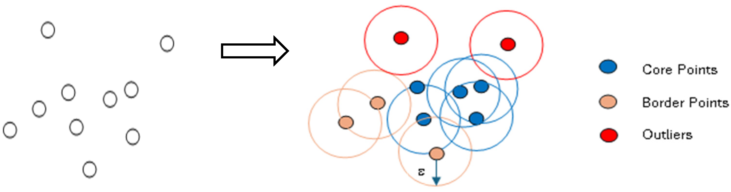

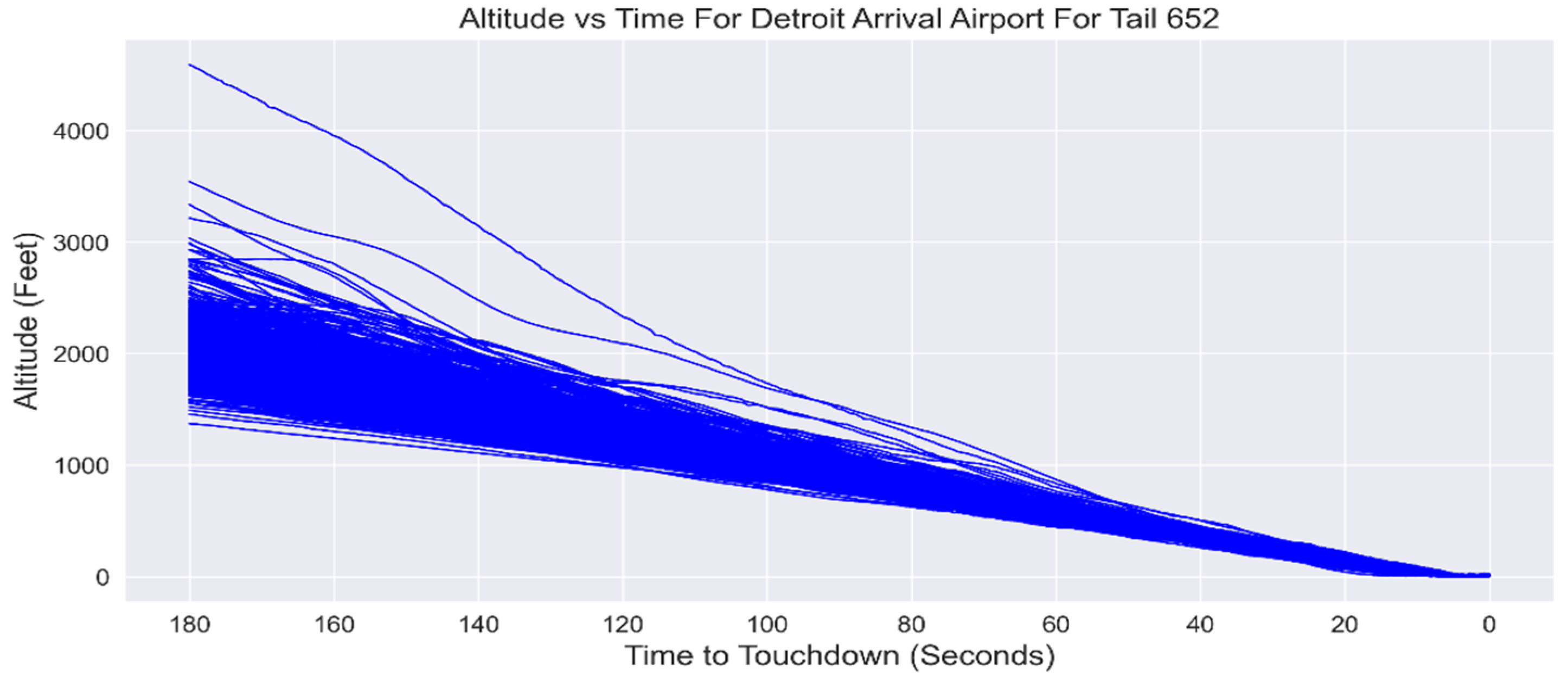

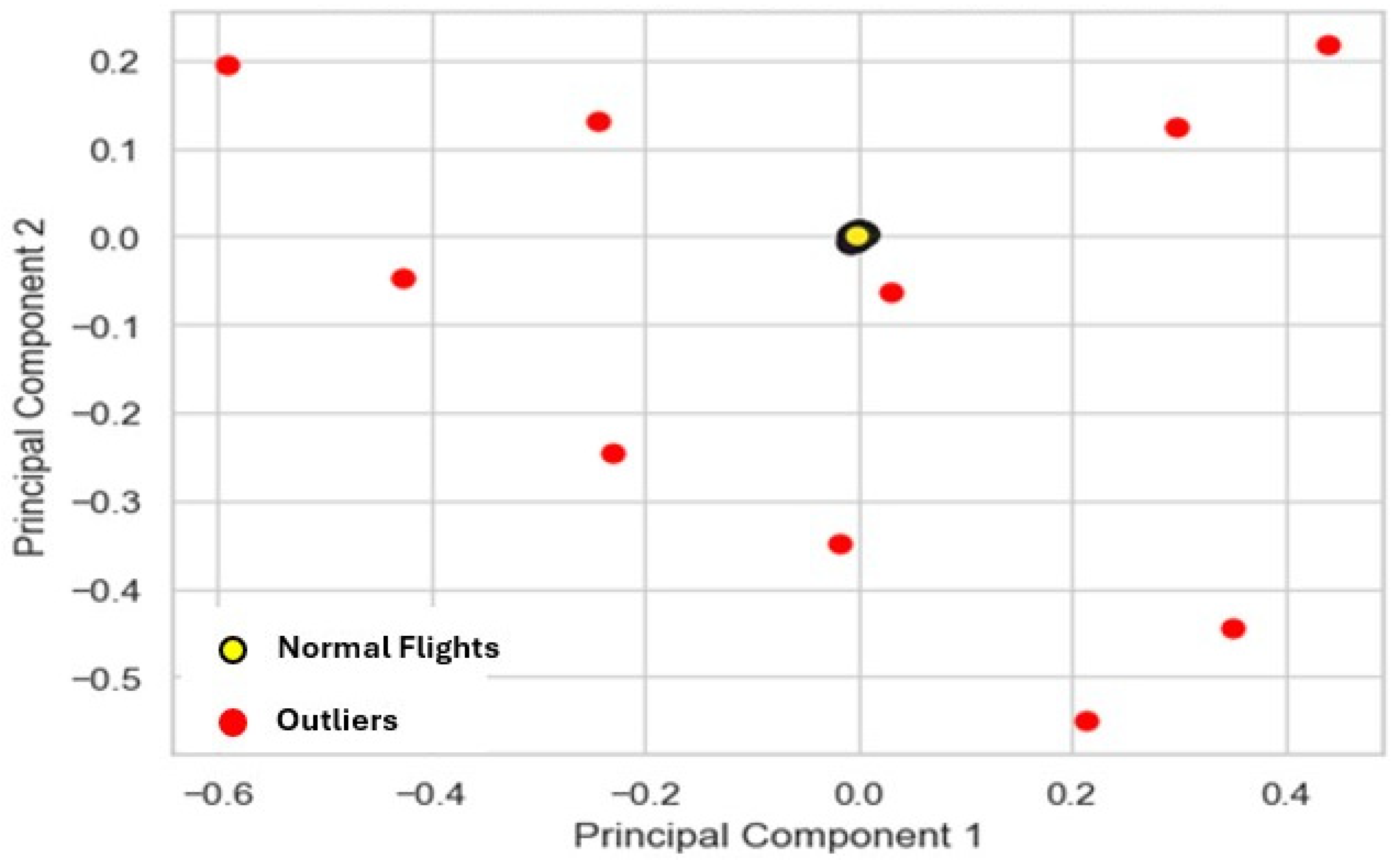
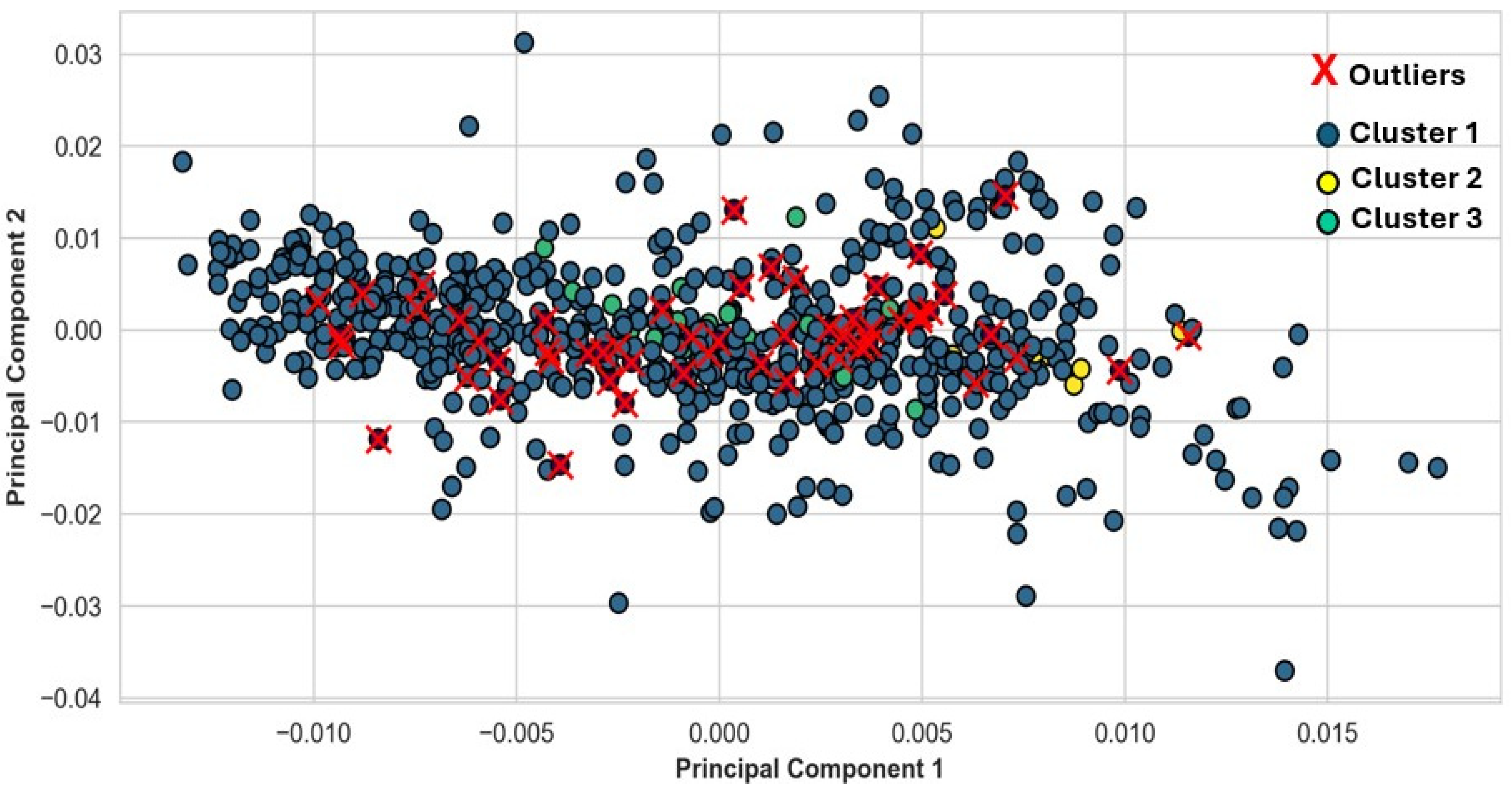

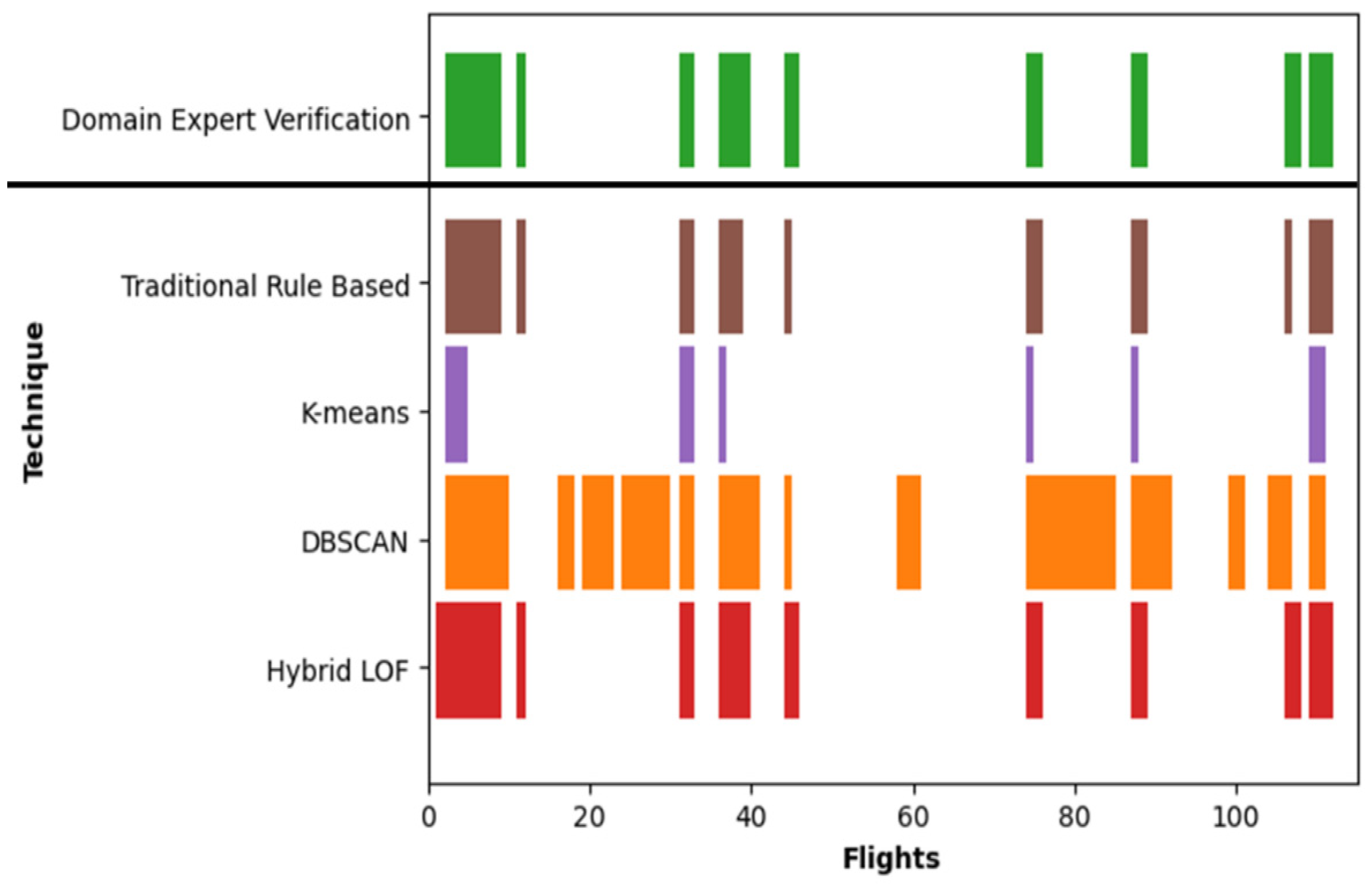
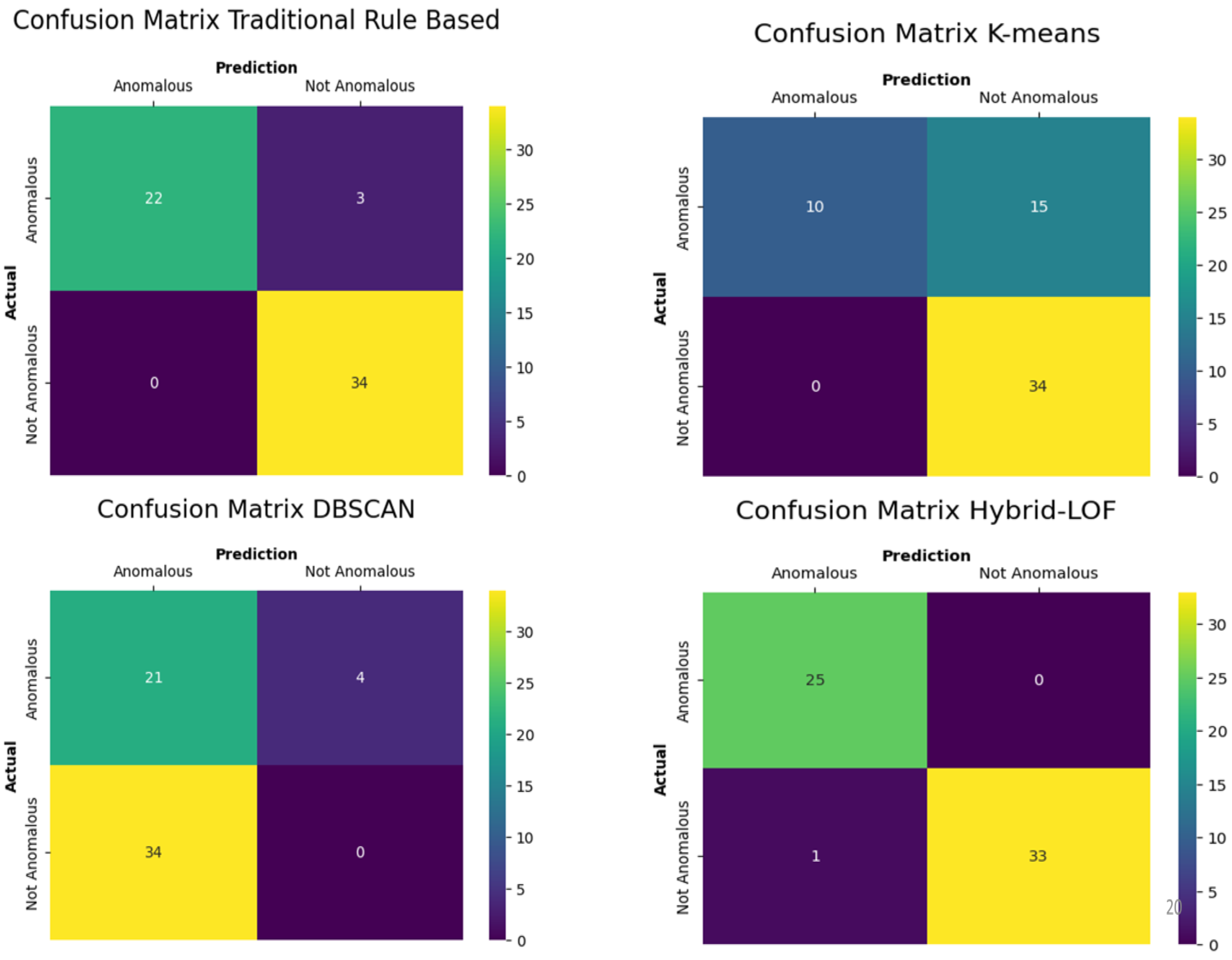

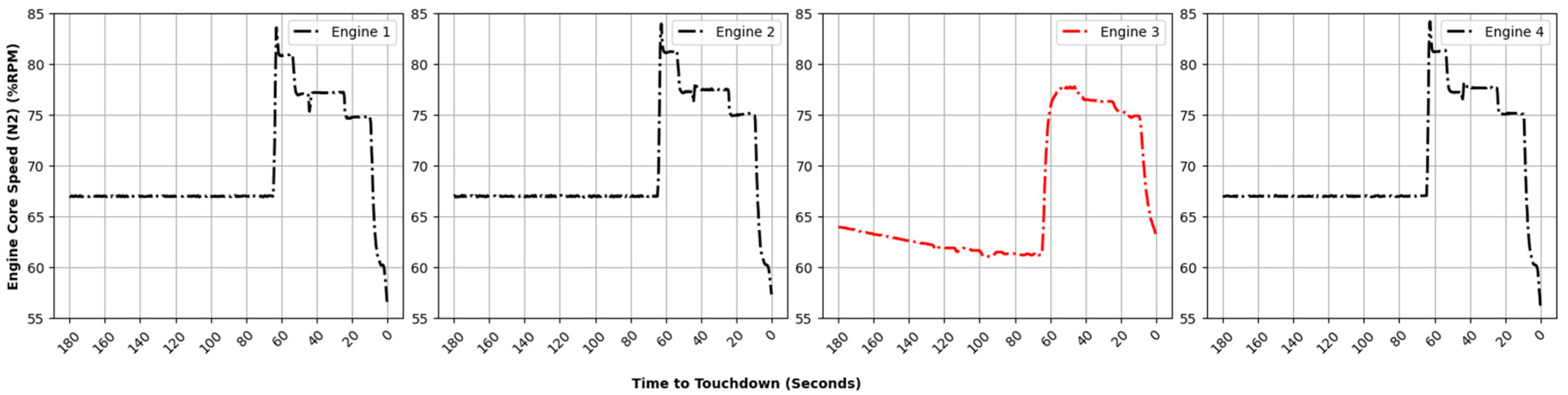

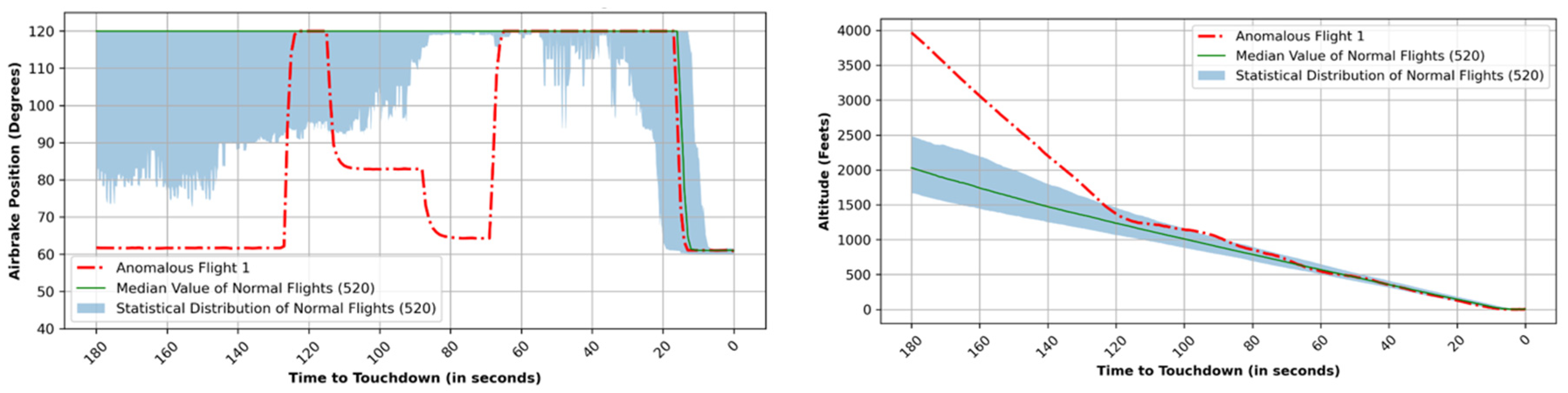
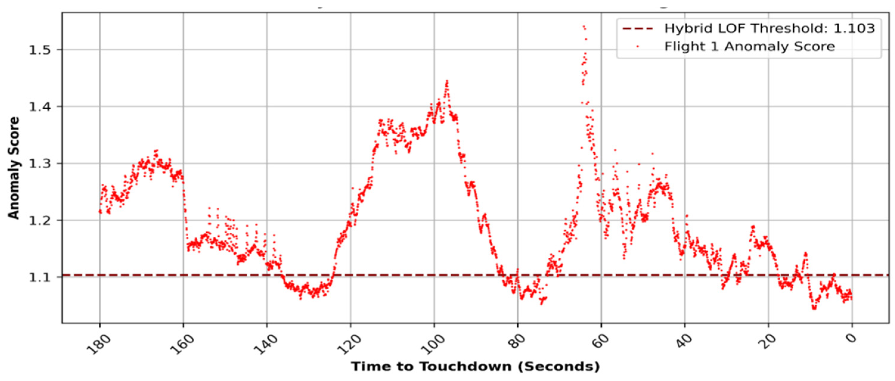
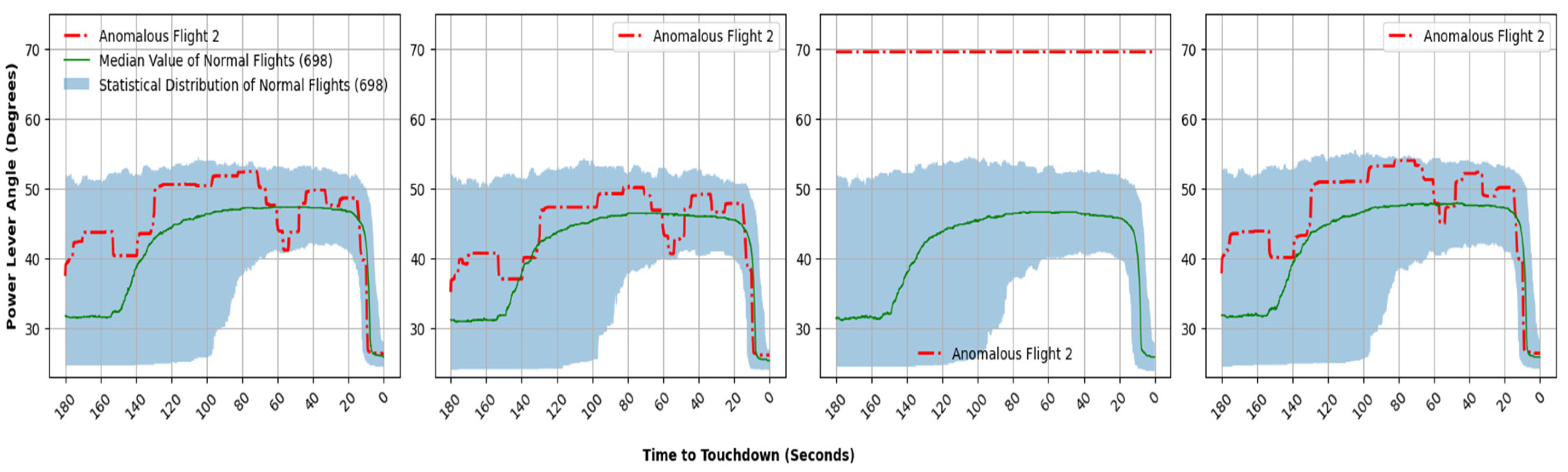
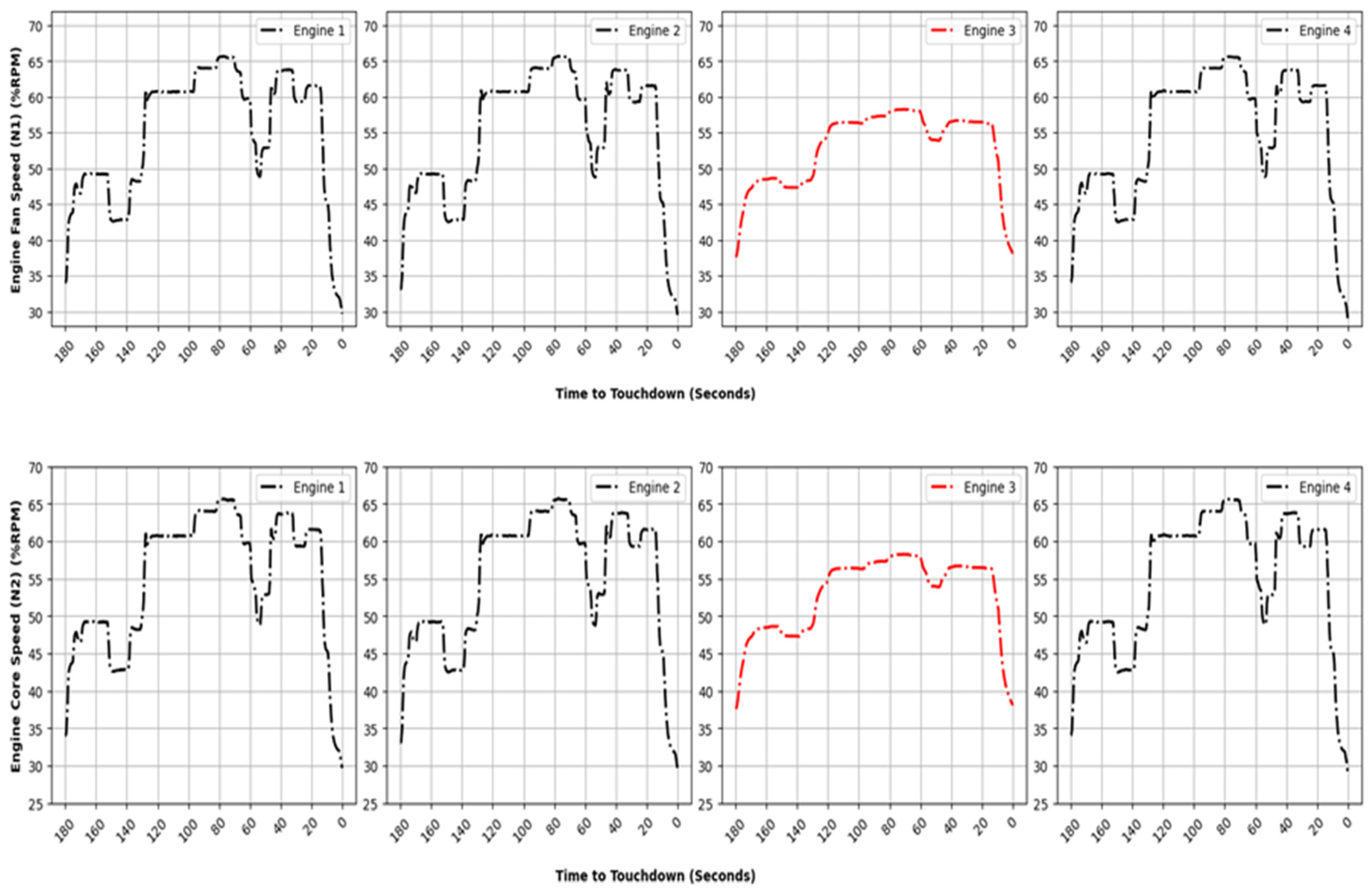

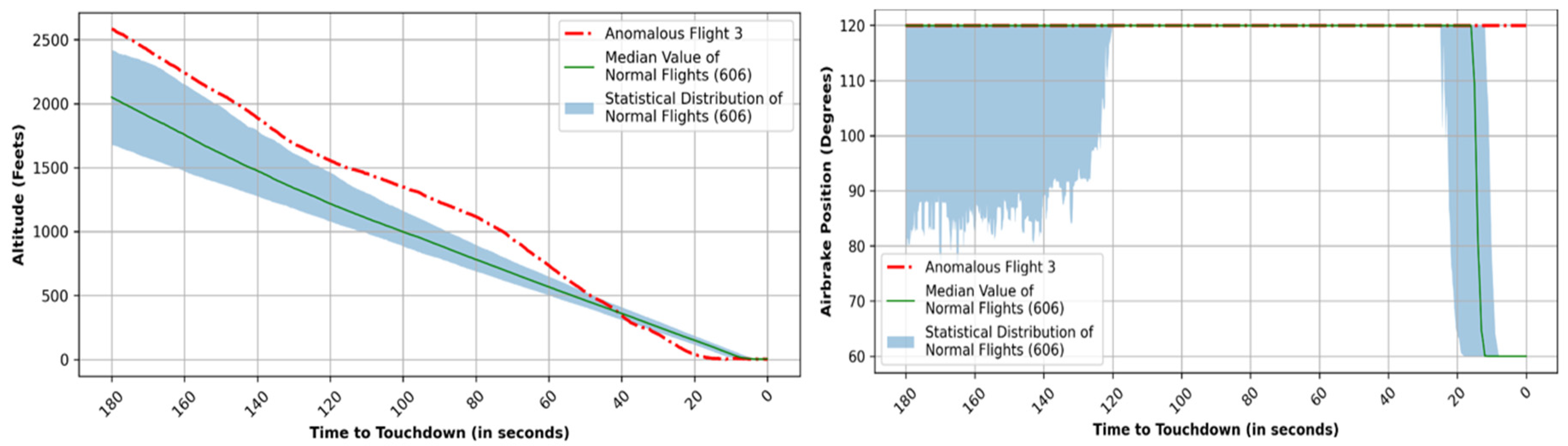

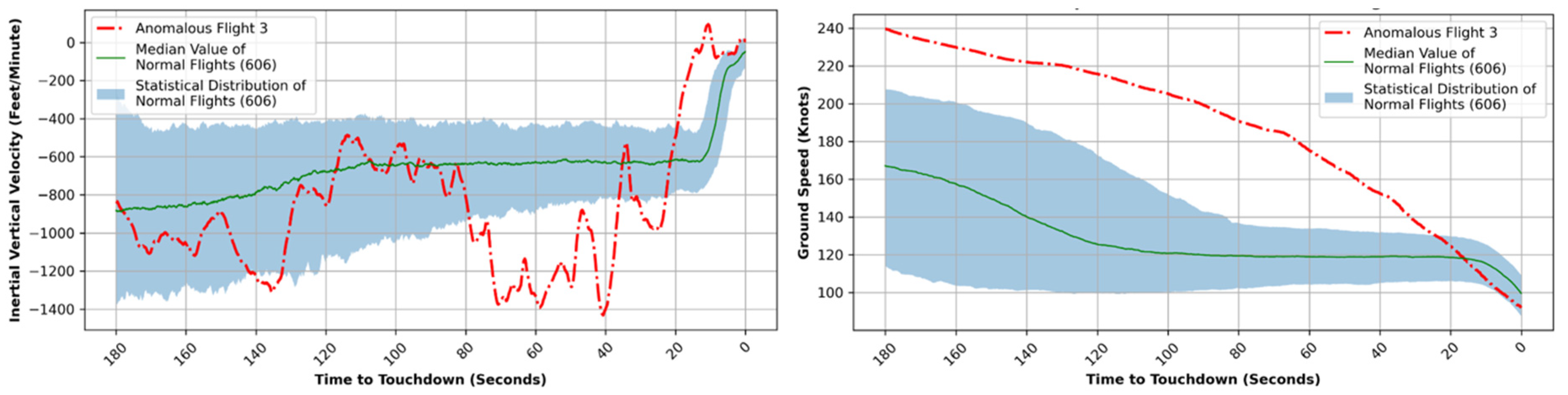
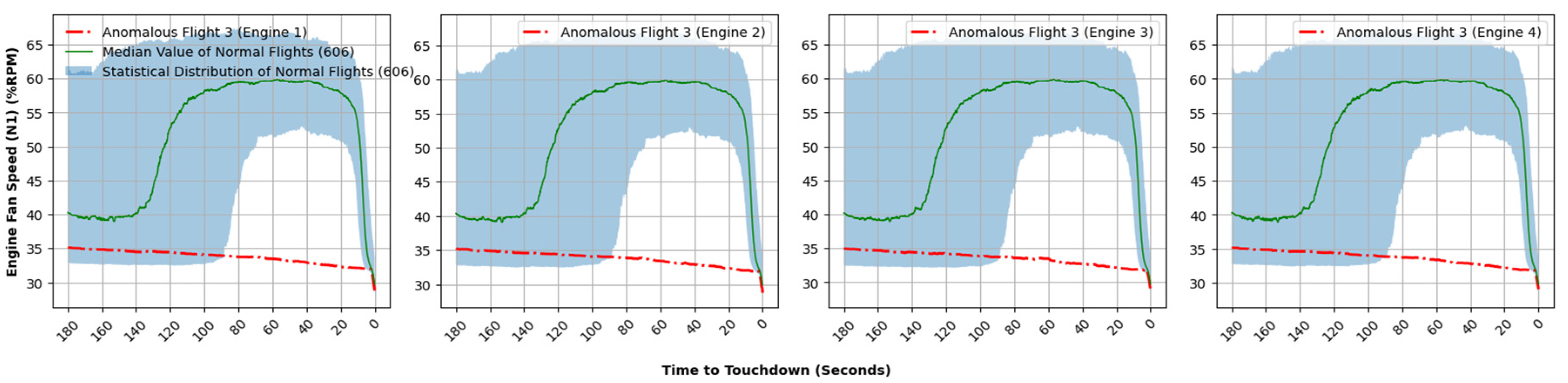

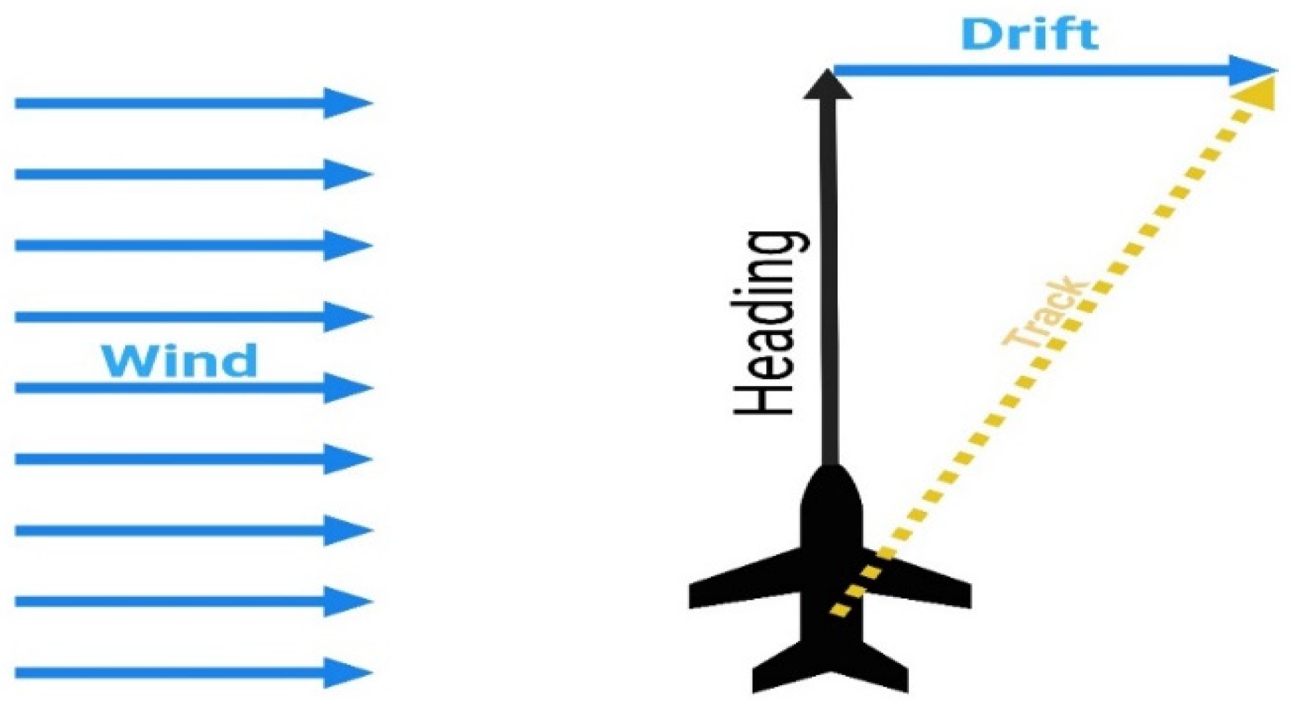
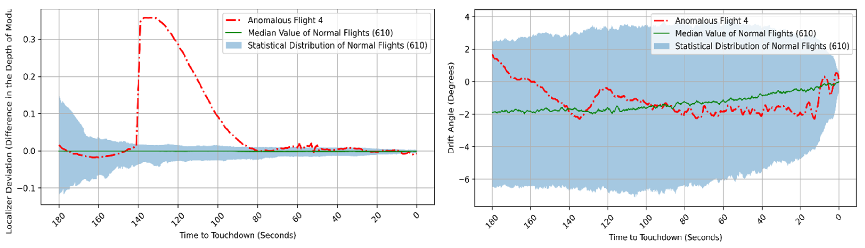


