Augmentation Method for X-Ray Pulsar Navigation Using Time Difference of Arrival and Range Measurement, Based on Polarization Encoded Pulse Position Modulation

Abstract

This paper addresses the use of the position difference between the reference satellite and the target spacecraft to improve X-ray pulsar navigation (XPNAV) for Earth orbit spacecraft. This is achieved by first installing an X-ray detector on the reference satellite whose position is accurately known. The position measurement error of the reference satellite, known as the correction value, is sent to the spacecraft through the X-ray communication (XCOM) link. It is hoped that the accuracy of the spacecraft state measurement can be improved by offsetting common errors of measurement. X-ray ranging observation between the reference satellite and the target spacecraft, obtained from XCOM, can accomplish high precision in distance measurements, which can supply precise information for XPNAV. A novel pulse position modulation (PPM) polarization encode and modulation mode is used to achieve difference time transmission and range measurement simultaneously. Through the information fusion of the difference timing observation and the ranging observation, the positioning accuracy of the spacecraft is improved further. With the aim of estimating the spacecraft’s errors in location and speed, an adaptive divided difference filter (ADDF) is applied to eliminate nonlinearity. Several simulation cases are designed to verify the proposed method. Numerical simulations show that, compared with the traditional timing observation, the difference timing and ranging method can improve the position estimation accuracy by 27% and the velocity estimation accuracy by 22%.

1. Introduction

X-ray pulsar navigation (XPNAV) is a novel method for spacecraft navigation. It can be used not only as an assistant to near-Earth space probes, such as satellite navigation systems, but can also supply the absolute time and spatial reference for deep space probes. It is an effective way to solve the problem of spacecraft autonomous navigation. The pulsar is far away from the solar system. The radiation direction of the pulsar observed at any point in the solar system is essentially the same, which can be approximated as a constant vector [1]. At present, the XPNAV system has a positioning precision within a range of several kilometers, which is far from its theoretical value [1]. There are several approaches to enhance the precision of XPNAV. Some authors have worked on improving the accuracy of the phase estimation of the cumulative pulse profile, including the time domain measurement method based on the bispectrum transform [2] or the Bayesian [3] or optimal frequency band algorithm [4]. Another solution was to acquire supplementary observational data from existing navigation systems or various space sources, for example, XPNAV and doppler system fusion [5,6], using the observational information of stars, planets or natural satellites [7,8,9,10]. In XPNAV, the time of arrival (TOA) is the essential observation, and the incremental phase of two instants of the satellite [11] or baseline vector angle between the two satellites [12] can also be used to improve the navigation precision. A more advanced filter algorithm, such as the adaptive difference Kalman filter (ADDF), is employed for navigation filtering. The aforementioned integration approach has certain potential, but it is limited in accuracy and is susceptible to noise interference. Moreover, a subsystem is required to manage these extra inputs, which enhances the complexity of the navigation system.

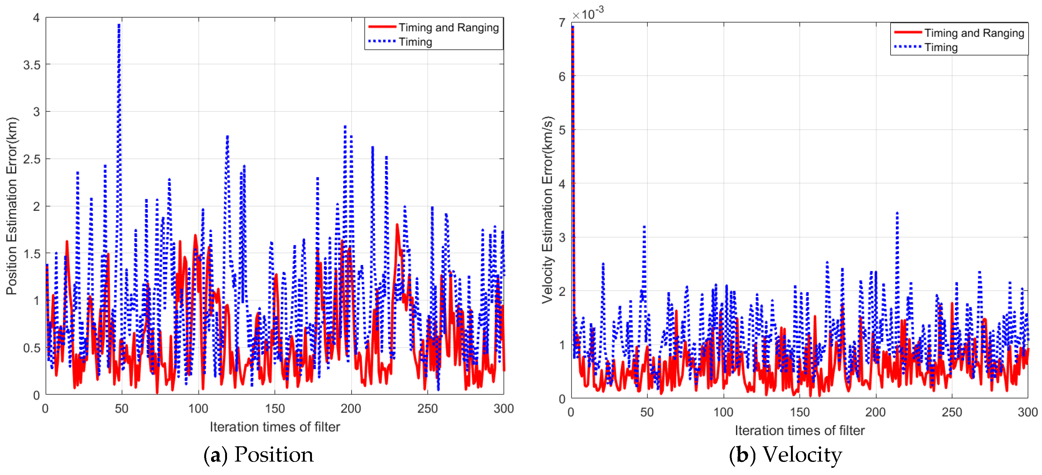
This paper presents an augmentation method for XPNAV by using the position difference between the reference satellite and the target spacecraft. The reference satellite, whose position is accurately known, is equipped with three detectors, two for navigation and one for communication. The accurate phase evolution model at the solar system barycenter (SSB) is calculated by using the accurate position information. First, the reference satellite receives the X-ray pulsar signal and obtains its time measurement value. Then, the time difference between the measurement value and the real time value is obtained. Next, it takes the time difference as the measurement error correction, which is sent to the spacecraft through the X-ray communication link. Finally, the spacecraft uses the time difference to correct its position information, so as to improve the navigation accuracy.

Currently, radio frequency or optical links are used to send information between spacecraft and Earth. X-ray communication (XCOM) has even greater advantages, as X-rays possess wavelengths that are considerably shorter ($0.01–10\mathrm{nm}$) than those of both radio and laser. Based on Planck’s radiation law, the number of photons is inversely related to the wavelength. This implies that, essentially, XCOM has the capability to transmit more data with the same level of transmission power. The X-rays can broadcast in narrower beams, reducing energy consumption during long-distance communication. On the other hand, the high-energy X-ray has a small loss of space transmission and diffraction [13]. The more photons the X-ray source emits, the higher the sensitivity of the detector. Last but not least, with the integration of communication and ranging, the X-ray detector can be shared and its utilization improved. Thus, information transmission can be realized with small volume and low power consumption. Moreover, the signal transmission is colorless and scattered, so the ranging accuracy is higher. We can use the ranging observation to make further improvements to the accuracy of XPNAV.

The concept of X-ray communication was first proposed in 2012 [14]. It is a new technology for space communication with X-rays, which have the characteristics of no attenuation, small spatial dispersion and interference and high ranging precision in deep space transmission [15,16]. The link power equation was established; also, the relationships between the transmitting speed, communication distance, bit error ratio and the transmission power were analyzed [17]. In one study [18], an idea for X-ray ranging based on XCOM was introduced and a detailed performance analysis was presented. Their experiments showed that X-ray ranging can provide accurate range measurement when the SNR of the ranging signal reaches a certain level, and it could serve as additional observations to augment XPNAV. A NASA experiment using a Modulated X-ray Source (MXS) and the X-ray telescope NICER demonstrated the possibility of the XCOM scheme with the transmission of GPS-like signals over a distance of 50 m [19].

To transmit the time difference from the reference satellite to the spacecraft, the code and modulation of the signal must be analyzed first. In one study [20], a space audio communication system based on X-rays with on–off keying (OOK) modulation was designed and tested. In another study [21], the impact of the OOK, pulse position modulation (PPM) and Quadrature Amplitude Modulation on the X-ray communication system performance was compared and analyzed. The OOK modulation system is straightforward and easy to implement, yet it suffers from low transmission efficiency. Furthermore, as the modulation rate increases, the transmission power decreases, limiting its capability for long-distance or ultra-high-speed communication. PPM modulation uses the position of the pulse to transmit information. It has the advantages of low average power and high transmission efficiency. But unfortunately, the anti-jamming ability is not strong enough and strict frame synchronization is needed. In space communication, many complex factors, such as space background light, channel interference and photon fluctuation, will affect the bit error rate (BER) of the system. In Reference [22], light polarization modulation with PPM is proposed, which can not only reduce the negative effects caused by atmospheric channels but also increase the communication code rate effectively in atmospheric laser communication. In Reference [23], the range information is communicated through circular polarization states, and simulation results indicate that the X-ray circularly polarized ranging technique could provide high-accuracy range measurement results. Consequently, the paper uses 4PPM circular polarization modulation to load ranging codes on X-ray photons to achieve space ranging. It is expected that this method can obtain larger communication capacity and smaller ranging error. Compared with the X-ray pulsar signal, the form and power of the X-ray ranging signal are controllable, and the design and application are flexible. The ranging and communication signal can be integrated and transmitted simultaneously. In addition, X-ray navigation and communication share the same X-ray detector, which is conducive to the miniaturization and integration of the system.

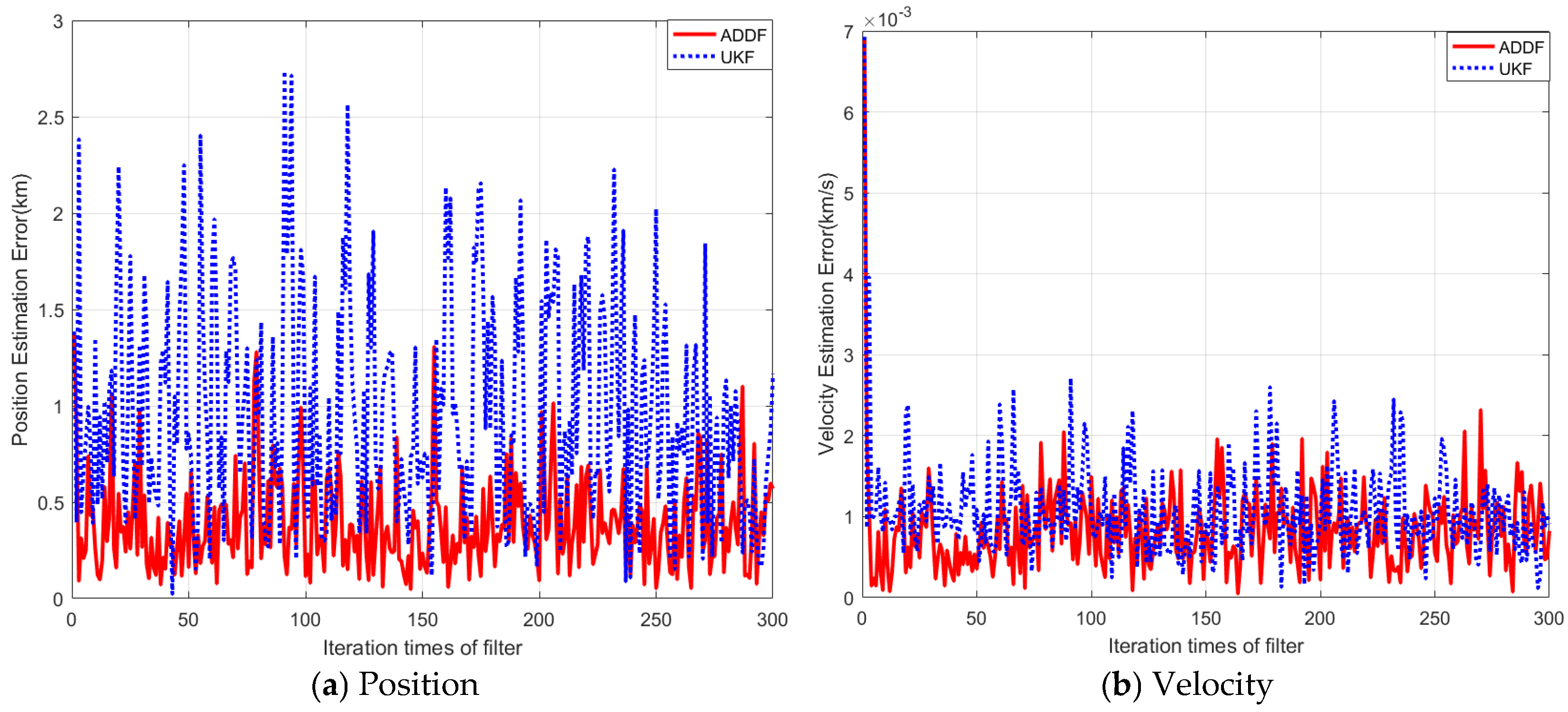
In XPNAV, the extended Kalman filter (EKF) and unscented Kalman filter (UKF) are frequently employed as filtering methods. The accuracy of the EKF is limited because it uses a first-order approximation of the system equations. The UKF eliminates the derivative calculation and offers greater precision compared to the EKF. However, the statistics of process noise are often unknown, and incorrect assumptions about it can result in the suboptimal performance of the filter. Thus, an adaptive divided difference filter (ADDF) is selected. The performance of the ADDF filter is demonstrated on a nonlinear system mentioned in the study by [24]. By adjusting the covariance of process noise, it can estimate the states of a nonlinear system with unknown process noise statistics. The paper demonstrates a substantial enhancement in navigation precision for augmented XPNAV when employing the ADDF.

The structure of this paper is outlined below. Section 2 will introduce the fundamental principles of augmented XPNAV. The pulsar timing and ranging observation equations are then established, and the ranging error is also analyzed theoretically. Then, the nonlinear ADDF algorithm, including the measurement model and orbital dynamic model, are described in Section 3. In Section 4, numerical simulations and their analyses are provided, followed by conclusions drawn in Section 5.

2. Principle of Augmented XPNAV System

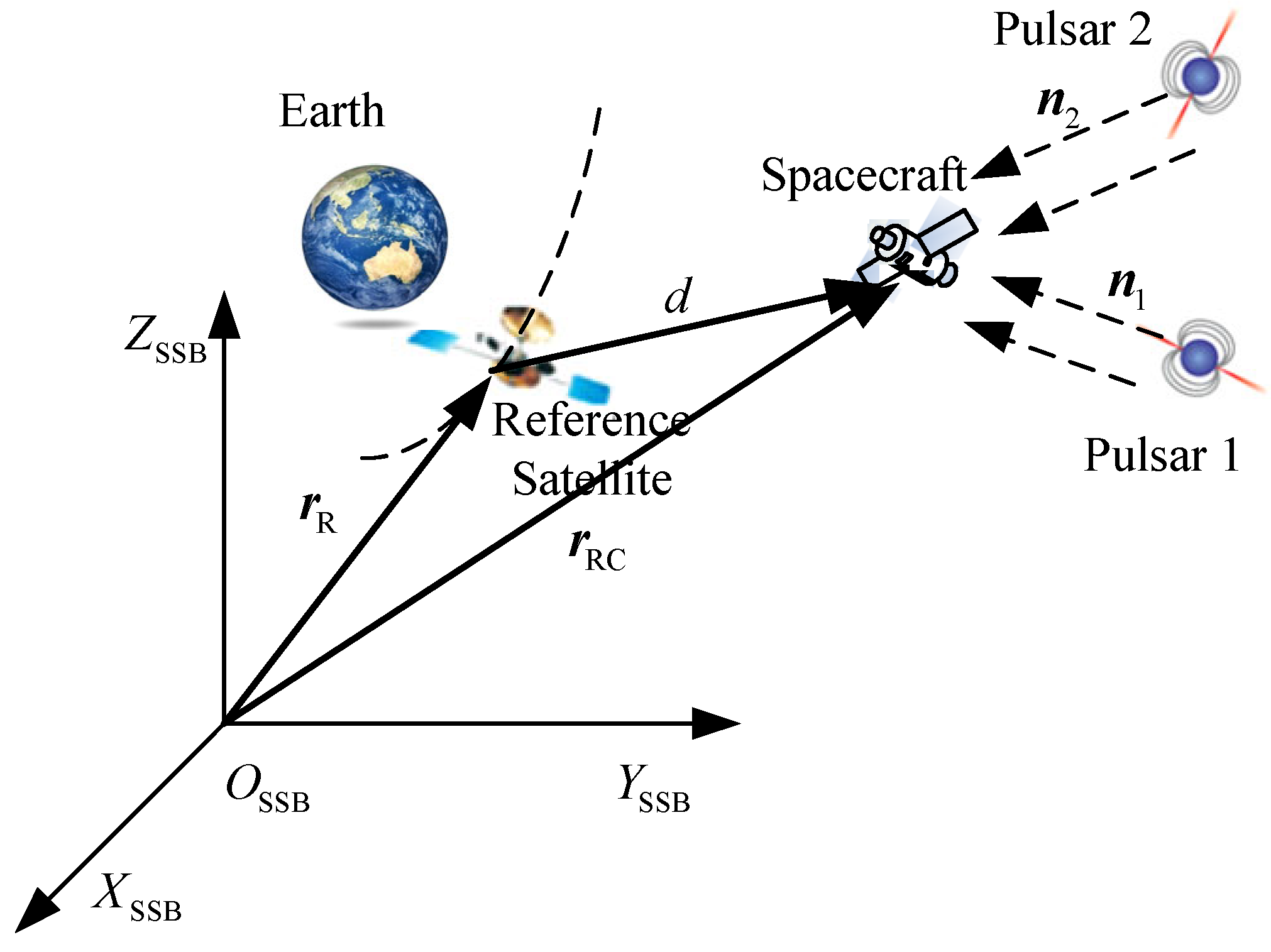
XPNAV determines the position and velocity of a spacecraft by utilizing the time difference of arrival (TDOA) of X-ray pulses between the spacecraft and the solar system barycenter (SSB). The traditional XPNAV method requires at least three different pulsars to confirm the three-dimensional position of the spacecraft. The differential augmented XPNAV method proposed in this paper needs to observe only two different pulsars, and the range between the Earth’s reference satellite and the target spacecraft is an additional observation. The celestial reference system is established in Figure 1.

The barycenter of the solar system $O_{SSB}$ is the origin, $Z_{SSB}$ is vertical with the celestial equator, $X_{SSB}$ is pointing to the vernal point defined by the standard epoch J2000.0 and $Y_{SSB}$ is pointing to the X–Z plane with regard to the right-hand rule. $r_{\mathrm{R}}$ and $r_{\mathrm{RC}}$ are the position vectors of the reference satellite and spacecraft with respect to SSB, respectively. $n_1$ and $n_2$ are the radiation directions of the pulsars. d is the range between the spacecraft and the reference satellite, which is used as an additional observation to augment the XPNAV.

The pseudo range measurement error of the reference satellite with respect to SSB can be considered to be approximately equal to that of the spacecraft to SSB. If the reference satellite uses its known position to estimate the measurement error and provides the measurement error to the spacecraft in the form of a correction value, it is expected to improve the position accuracy of the spacecraft.

2.1. Pulsar Timing Observation

Let $r_{\mathrm{R}}={[x_{\mathrm{R}} y_{\mathrm{R}} z_{\mathrm{R}}]}^{\mathrm{T}}$ be the reference satellite’s estimation position vector. The X-ray detector installed on the reference satellite receives the X-ray photon and records its time of arrival. The pulsar phase revolution model is established at the SSB to predict the TOA of the pulsar pulse. The measured pulse TOA at the reference satellite should be transformed to the same time framework at the SSB. By comparing the predicted TOA of pulsar pulse with the measured TOA, the position of the reference satellite can be obtained. Taking into account that the gravity of the Sun is the main gravity source in the solar system, the geometric and relativistic effects cannot be ignored. The simplified TOA transfer equation from the reference satellite to the SSB is given by [1,25].

$$\begin{array}{cc}{t}_{\mathrm{SSB}}-t_{\mathrm{R}}=& {\displaystyle \frac{n\cdot r_{\mathrm{R}}}{c}}+{\displaystyle \frac{1}{2c{\mathrm{D}}_0}}\left[{\left(n\cdot r_{\mathrm{R}}\right)}^2-{‖r_{\mathrm{R}}‖}^2+2\left(n\cdot b\right)\left(n\cdot r_{\mathrm{R}}\right)-2\left(b\cdot r_{\mathrm{R}}\right)\right] +\hfill \\ & {\displaystyle \frac{2{\mu }_{\mathrm{s}}}{c^3}}\ln \left|{\displaystyle \frac{\mathit{n}\cdot r_{\mathrm{R}}+n\cdot b+‖r_{\mathrm{R}}‖+‖b‖}{n\cdot b+‖b‖}}\right|\hfill \end{array}$$

(1)

where $t_{\mathrm{SSB}}$ and $t_{\mathrm{R}}$ are the TOAs of the SSB and the reference satellite, respectively. $r_{\mathrm{R}}$ and $b$ are the position vectors of the reference satellite and the Sun with respect to SSB, respectively. $\mathit{n}$ is the radiation direction of the pulsar and ${\mu }_{\mathrm{s}}$ is the solar gravitational constant. ${\mathrm{D}}_0$ is the distance between the first pulsar and SSB. c is the speed of light.

$r_{\mathrm{R}}$ is calculated using the TOA of the pulsar signal. It contains various errors stemming from the timing, phase comparison and so on. In Earth’s orbit, these measurement errors can be considered as approximations. So, if these errors can be extracted, they can be used to correct the position estimation of other satellites.

Suppose $r_{\mathrm{R}0}={[x_{\mathrm{R}0} y_{\mathrm{R}0} z_{\mathrm{R}0}]}^{\mathrm{T}}$ is the precise position vector of the reference satellite, which is known by ground measurement equipment. With the exact position vector, the exact TOA transfer equation from the reference satellite to the SSB is obtained.

$$\begin{array}{cc}\hfill t_{\mathrm{SSB}}-t_{\mathrm{R}0}=& {\displaystyle \frac{n\cdot r_{\mathrm{R}0}}{c}}+{\displaystyle \frac{1}{2c{\mathrm{D}}_0}}\left[{\left(n\cdot r_{\mathrm{R}0}\right)}^2-{‖r_{\mathrm{R}0}‖}^2+2\left(n\cdot b\right)\left(n\cdot r_{\mathrm{R}0}\right)-2\left(b\cdot r_{\mathrm{R}0}\right)\right] +\hfill \\ & {\displaystyle \frac{2{\mu }_{\mathrm{s}}}{c^3}}\ln \left|{\displaystyle \frac{\mathit{n}\cdot r_{\mathrm{R}0}+n\cdot b+‖r_{\mathrm{R}0}‖+‖b‖}{n\cdot b+‖b‖}}\right|\hfill \end{array}$$

(2)

Subtracting Equation (2) from Equation (1) yields the time difference between the actual and observation times of the reference satellite, which can be expressed as follows:

$$\begin{array}{cc}\hfill \delta t_{\mathrm{i}}& =(t_{\mathrm{SSB}}-t_{\mathrm{R}})-(t_{\mathrm{SSB}}-t_{\mathrm{R}0})\hfill \\ & ={\displaystyle \frac{n\cdot \delta \tilde{r}}{c}}+{\displaystyle \frac{1}{2c{\mathrm{D}}_0}}\left[\left(n\cdot (r_{\mathrm{R}}+r_{\mathrm{R}0})\right)(n\cdot \delta \tilde{r})-(‖r_{\mathrm{R}}‖+‖r_{\mathrm{R}0}‖)‖\delta \tilde{r}‖+2\left(n\cdot b\right)\left(n\cdot \delta \tilde{r}\right)-2\left(b\cdot \delta \tilde{r}\right)\right] +\hfill \\ & {\displaystyle \frac{2{\mu }_{\mathrm{s}}}{c^3}}\ln \left|1+{\displaystyle \frac{\mathit{n}\cdot \delta \tilde{r}+‖\delta \tilde{r}‖}{\mathit{n}\cdot r_{\mathrm{R}0}+n\cdot b+‖r_{\mathrm{R}0}‖+‖b‖}}\right|\hfill \end{array}$$

(3)

where $\delta \tilde{r}=r_{\mathrm{R}}-r_{\mathrm{R}0}$. $r_{\mathrm{R}}$ is measured using the TOA of the pulsar signal and $r_{\mathrm{R}0}$ is the position vector of the reference satellite. So, $\delta \tilde{\mathit{r}}$ can be treated as the differential correction value. Generally, $‖r_{\mathrm{R}}‖$ is in the order of ${10}^8 \mathrm{km}$ and $‖b‖$ is in the order ${10}^5 \mathrm{km}$. However, in the solar system $D_0$ is in the order of ${10}^{14} \mathrm{km}$. ${\mu }_{\mathrm{s}}$ is $1.327\mathrm{e}+11{ \mathrm{km}}^3/{\mathrm{s}}^2$. At present, the positioning accuracy of X-ray pulsar is better than $10 \mathrm{km}$. Assuming $\delta \tilde{r}$ is $10 \mathrm{km}$, the values of $(‖r_{\mathrm{R}}‖+‖r_{\mathrm{R}0}‖)‖\delta \tilde{r}‖/D_0$ with the order of magnitude ${10}^{-5} \mathrm{km}$ and $\left(n\cdot b\right)\left(n\cdot \delta \tilde{r}\right)/D_0$ with the order of magnitude ${10}^{-6} \mathrm{km}$ are negligible. The values of $(n\cdot \delta \tilde{r}+‖\delta \tilde{r}‖)/(n\cdot r_{\mathrm{R}0}+n\cdot b+‖r_{\mathrm{R}0}‖+‖b‖)$ are in the order of magnitude ${10}^{-7} \mathrm{km}$, so that $2{\mu }_s\ln \left|1+(n\cdot \delta \tilde{r}+‖\delta \tilde{r}‖)/(n\cdot r_{\mathrm{R}0}+n\cdot b+‖r_{\mathrm{R}0}‖ + ‖b‖)\right|/c^3$ can be considered equal to $0$. Thus, Equation (3) can be rewritten as

$$\delta t_{\mathrm{i}}={\displaystyle \frac{n\cdot \delta \tilde{r}}{c}}$$

(4)

Suppose $r_{\mathrm{RC}}$ is the estimation position vector of the spacecraft with respect to SSB and $r_{\mathrm{RC}0}$ is the actual position vector of the spacecraft with respect to SSB.

$$\delta t_{\mathrm{j}}={\displaystyle \frac{n\cdot \delta {\tilde{r}}_{\mathrm{SC}}}{c}}$$

(5)

where $\delta {\tilde{r}}_{\mathrm{SC}}=r_{\mathrm{SC}}-r_{\mathrm{SC}0}$.

At present, the positioning accuracy of X-ray pulsar is better than $10 \mathrm{km}$, assuming $\delta \tilde{r}$ is $10 \mathrm{km}$. For the reference satellite and spacecraft, they observe the same pulsar and have the same phase revolution model. From Figure 1, the distance between the reference satellite and spacecraft can be written as $d=\left|r_{\mathrm{R}}-r_{\mathrm{RC}}\right|$. Because they belong to the same Earth satellite, the maximum distance between them is in the order of ${10}^5 \mathrm{km}$. Moreover, the pulsar is far away from the solar system (in the order of ${10}^{14} \mathrm{km}$), which is far greater than the distance between the reference satellite and spacecraft. The radiation direction of the pulsar observed at any point in the solar system is essentially the same, which can be approximated as a constant vector. The influence of relativistic effects on $d$ is negligible. Therefore, $\delta \tilde{r}$ can be considered to be approximately equal to $\delta {\tilde{r}}_{\mathrm{SC}}$. It can be considered that the measurement errors of different spacecrafts in the solar system are equal, that is, $\delta t_{\mathrm{i}}=\delta t_{\mathrm{j}}$. So, we can use the reference satellite’s known precise position to obtain the measurement error; then, as a correction, the measurement error is transmitted to the spacecraft and the common error terms in the TOA can be eliminated in the spacecraft. This paper takes advantage of the difference time to improve the state accuracy of spacecraft.

Based on the above analysis, the spacecraft measures the TOA, which can be used to determine the position by calculating the flying time of the pulse between the spacecraft and SSB.

$$\begin{array}{cc}\hfill t_{\mathrm{SSB}}-t_{\mathrm{SC}}=& {\displaystyle \frac{n\cdot r_{\mathrm{SC}}}{c}}+{\displaystyle \frac{1}{2c{\mathrm{D}}_0}}\left[{\left(n\cdot r_{\mathrm{SC}}\right)}^2-{‖r_{\mathrm{SC}}‖}^2+2\left(n\cdot b\right)\left(n\cdot r_{\mathrm{SC}}\right)-2\left(b\cdot r_{\mathrm{SC}}\right)\right] +\hfill \\ & {\displaystyle \frac{2{\mu }_{\mathrm{s}}}{c^3}}\ln \left|{\displaystyle \frac{\mathit{n}\cdot r_{\mathrm{SC}}+n\cdot b+‖r_{\mathrm{SC}}‖+‖b‖}{n\cdot b+‖b‖}}\right|\hfill \end{array}$$

(6)

where $r_{\mathrm{RC}}$ is the estimation position vector of the spacecraft with respect to SSB.

The time correction $\delta t=\delta t_{\mathrm{i}}=\delta t_{\mathrm{j}}$ is transmitted to the spacecraft through XCOM. Then, the spacecraft recovers the time correction from the communication data. Subtracting the time correction from the measurement time, the accurate TOA is obtained.

$$\begin{array}{l}{t}_{\mathrm{SSB}}-t_{\mathrm{SC}}-\delta t={\displaystyle \frac{\mathit{n}\cdot ({\mathit{r}}_{\mathrm{SC}}-\delta {\tilde{\mathit{r}}}_{\mathrm{SC}})}{c}}+{\displaystyle \frac{1}{2c{\mathrm{D}}_0}}\left[{\left(n\cdot r_{\mathrm{SC}}\right)}^2-{‖r_{\mathrm{SC}}‖}^2+2\left(n\cdot b\right)\left(n\cdot r_{\mathrm{SC}}\right)-2\left(b\cdot r_{\mathrm{SC}}\right)\right] +\\ {\displaystyle \frac{2{\mu }_{\mathrm{s}}}{c^3}}\ln \left|{\displaystyle \frac{\mathit{n}\cdot r_{\mathrm{SC}}+n\cdot b+‖r_{\mathrm{SC}}‖+‖b‖}{n\cdot b+‖b‖}}\right|\end{array}$$

(7)

where $\delta {\tilde{r}}_{\mathrm{SC}}=r_{\mathrm{SC}}-r_{\mathrm{SC}0}$. Equation (7) is rewritten as

$$t_{\mathrm{SSB}}-t_{\mathrm{SC}}-\delta t={\displaystyle \frac{\mathit{n}\cdot {\mathit{r}}_{\mathrm{SC}0}}{c}}+\Delta t_{\mathrm{SM}}$$

(8)

where

$$\Delta t_{\mathrm{SM}}={\displaystyle \frac{1}{2c{\mathrm{D}}_0}}\left[{\left(n\cdot r_{\mathrm{SC}}\right)}^2-{‖r_{\mathrm{SC}}‖}^2+2\left(n\cdot b\right)\left(n\cdot r_{\mathrm{SC}}\right)-2\left(b\cdot r_{\mathrm{SC}}\right)\right]+{\displaystyle \frac{2{\mu }_{\mathrm{s}}}{c^3}}\ln \left|{\displaystyle \frac{\mathit{n}\cdot r_{\mathrm{SC}}+n\cdot b+‖r_{\mathrm{SC}}‖+‖b‖}{n\cdot b+‖b‖}}\right|.$$

2.2. Ranging Observation Based on XCOM

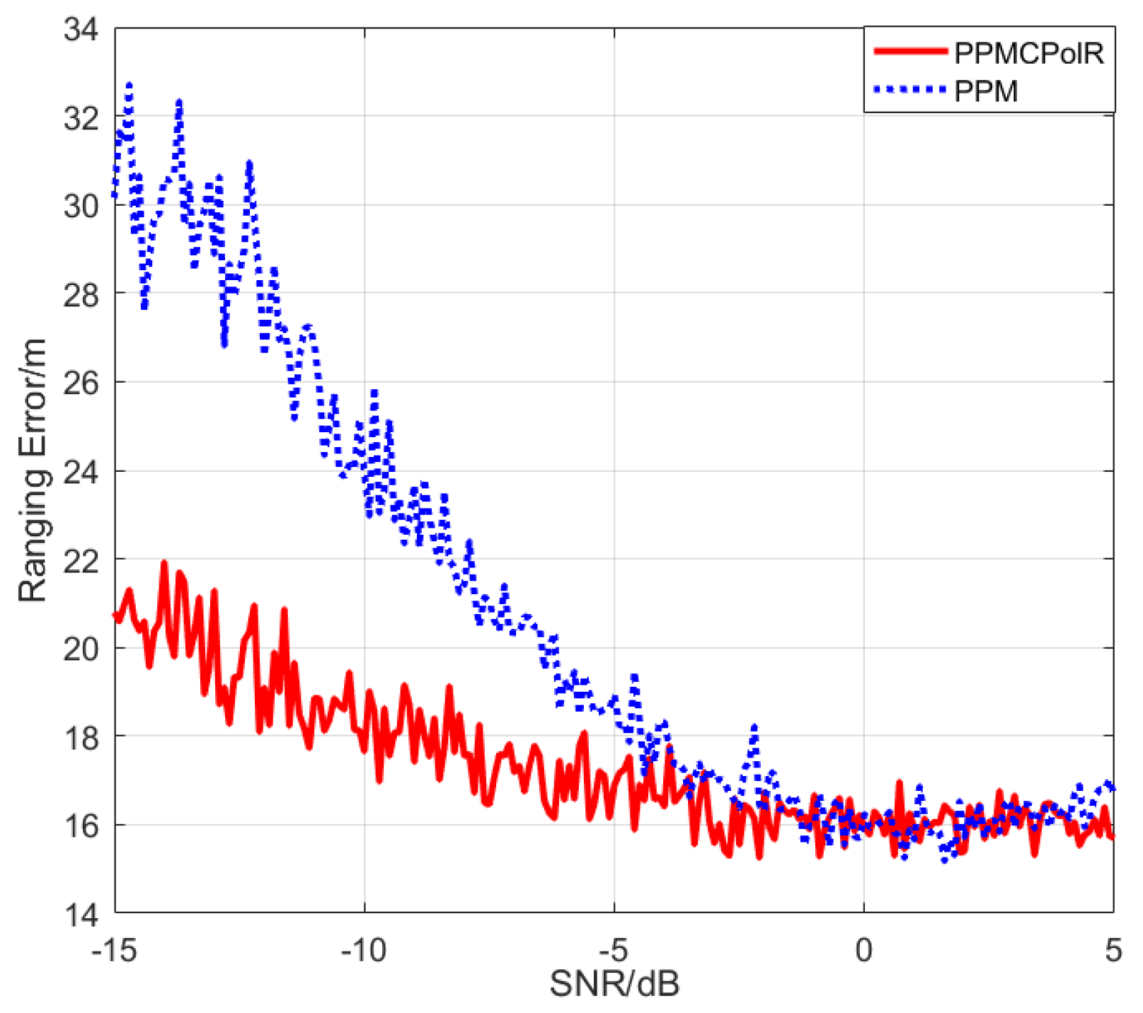
In this paper, the range between the spacecraft and the reference satellite near the Earth is utilized as an observation to improve the performance of XPNAV. For the range measurement, OOK or PPM can be used in the space X-ray communication system, but space background light, channel interference, photon fluctuation and various noises of the detector will affect the BER. The idea of X-ray PPM polarization coding is proposed, which can reduce the influence of deep space environment factors, improve X-ray communication capacity and effectively suppress the BER of the system. The principle of the PPM polarization ranging method based on XCOM will be illustrated in the following sections.

2.2.1. Principle of PPM Polarization Modulation

In the XCOM system, information is loaded on X-ray photons. At present, the main method is to transfer digital signals by modulating the intensity of light. Polarization is the inherent property of light, and the polarization state is an independent parameter of light, reflecting the vector characteristics of light. There is a strict phase relationship between the vibration components of the fully polarized light along different directions. The overall drift of the polarized state will not change the relative position of each polarized state, so it has a strong anti-interference ability. Therefore, the polarization state of signal light can be modulated, and different polarization states can be used to carry different information, for example, two orthogonal circular polarization states carry 2-bit information, and four elliptical polarization states to carry 4-bit information. The output signal after polarization modulation is an optical pulse with equal intensity but different polarization states.

PPM maps n-bit binary data sets to one slot in a frame [26]. The transmitted information is represented by the slot position of the optical pulse. If the n-bit data group is written as $M=(m_1,m_2,\dots ,m_n)$, $l$ indicates the slot position; then, the mapping coding relationship of the monopulse PPM modulation can be written as $l=m_1+2m_2+\dots +2^{n-1}{m}_n$, $l\in (0,1,2,\dots ,2^{n-1})$, that is

$$S_i(t)=\left\{\begin{array}{cc}{P}_{\mathrm{C}} & \hfill l{T}_C<t<(l+1)T_C\\ 0& \hfill others\end{array}\right.$$

(9)

where $i=0,1,\dots ,(2^n-1)$, $S_i(t)$ is the modulated signal, $P_{\mathrm{C}}$ is the pulse power and $T_{\mathrm{C}}$ is the slot duration.

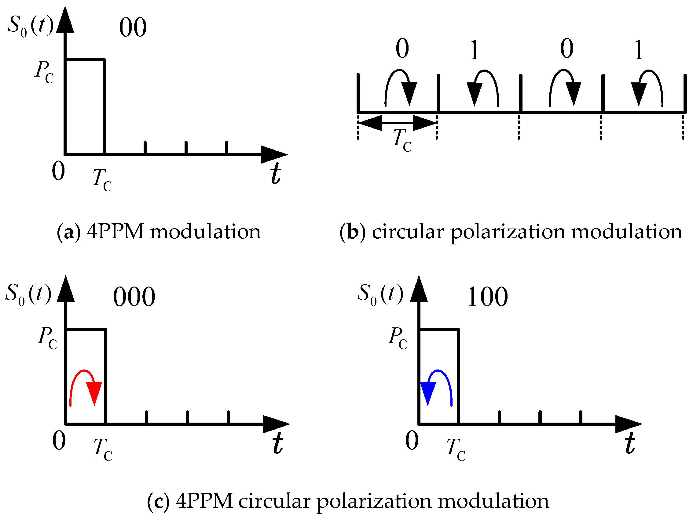
For example, to the 4PPM modulation, $n=2$. If $M=(0,0)$, then $l=0$; $M=(1,0)$, $l=1$; $M=(0,1)$, $l=2$; and $M=(1,1)$, $l=3$. $l=0$ matches the 0th slot; similarly, $l=1,2,3$ show the 1st, 2nd and 3rd slot positions, respectively. As shown in Figure 2a, $S_0(t)$ indicates the modulation signal corresponding to the 0th slot. The amount of information that the 4PPM modulation can represent is 2 bits. The total number of bits of information transmitted by an L-bit PPM modulation signal is ${\log }_{2}L$.

The method of 4PPM circular polarization modulation proposed in this paper is to add circular polarization information on the basis of 4PPM modulation.

We can express the circularly polarized signal as [27,28,29].

$$S_x(t)=\left\{S_{\mathrm{j}}(A_x,A_y,\psi (k))\right\}, j=0,1,2,3$$

(10)

where $A_x$ and $A_y$ are the amplitudes of the light vector components and $\psi (k)$ is the phase error between the two light vector components, which can be defined as

$$\psi (k)=\left\{\begin{array}{cc}\begin{array}{c}\begin{array}{cc}{\displaystyle \frac{\pi }{2}}+2a\pi & k=1\end{array}\\ \begin{array}{cc}-{\displaystyle \frac{\pi }{2}}+2a\pi & k=0\end{array}\end{array}& a\in Z\end{array}\right.$$

(11)

When $k=1$, $\psi (k)$ represents the left-hand polarization state. When $k=0$, it is the right-hand polarization state. As shown in Figure 2b, the amount of information that circular polarization modulation can represent is 1 bit.

For example, the pulses mapped at the 0th slot position can be represented by left-hand or right-hand polarization. As shown in Figure 2c, when the polarization state is left-hand, the signal can be expressed as $(1,0,0)$, while if the polarization state is right-hand, the signal can be expressed as $(0,0,0)$. For the pulses at the rest of the slot positions, the signal can be expressed in the same way. It can be shown that the total amount of information transmitted by the 4PPM circularly polarized modulation signal is 3 bits. Generally speaking, the total amount of information transmitted by the L-bit PPM circular polarization modulation signal is $1+{\log }_{2}L$.

2.2.2. Ranging Observation

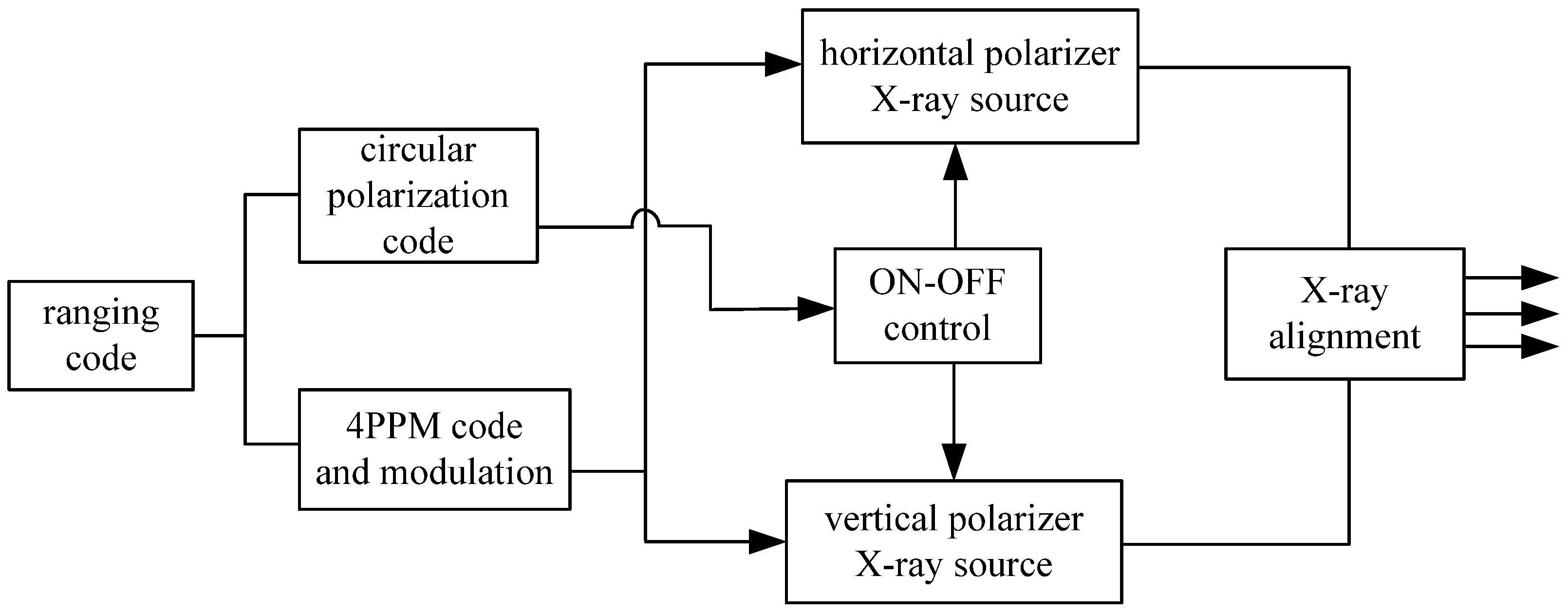
In this paper, the XCOM range measurement is a two-way measurement. The ranging sequence is transmitted to the slave station and sent back to the master station. The beam splitter and synthesizer are available devices in optical communication [13,22], but both devices cannot realize the synthesis and separation of X-ray photons. The structure of modulation and demodulation for the X-ray ranging signal is explained below. The block diagram of the 4PPM polarization modulation is shown in Figure 3.

First, the ranging code is divided into groups of 3 bits. Then, the lower 2 bits are encoded by 4PPM and the higher 1 bit is encoded by circular polarization, the ON–OFF control unit is used to select horizontal or vertical polarization modulation for the X-ray source and finally, after beam combination and collimation, the modulated signal is transmitted.

The ranging sequence is defined as

$$r(t)={\displaystyle \sum _i{c}_{i}g(t-i{T}_{\mathrm{C}})}$$

(12)

where $\left\{c_i\right\}, i\in N, i<M$ is the ranging code, M is its length, $T_{\mathrm{C}}$ is the slot duration and $\mathrm{g}(t)$ is the gate signal, which can be defined as

$$\mathrm{g}(t)=\left\{\begin{array}{cc}1 \hfill & \hfill t\in [0,T_{\mathrm{C}}]\\ 0\hfill & \hfill others\end{array}\right.$$

(13)

The T4B pseudo-noise code is selected as the ranging code, which can provide high ranging accuracy. The m-sequence is chosen as the synchronization sequence of the PPM coding.

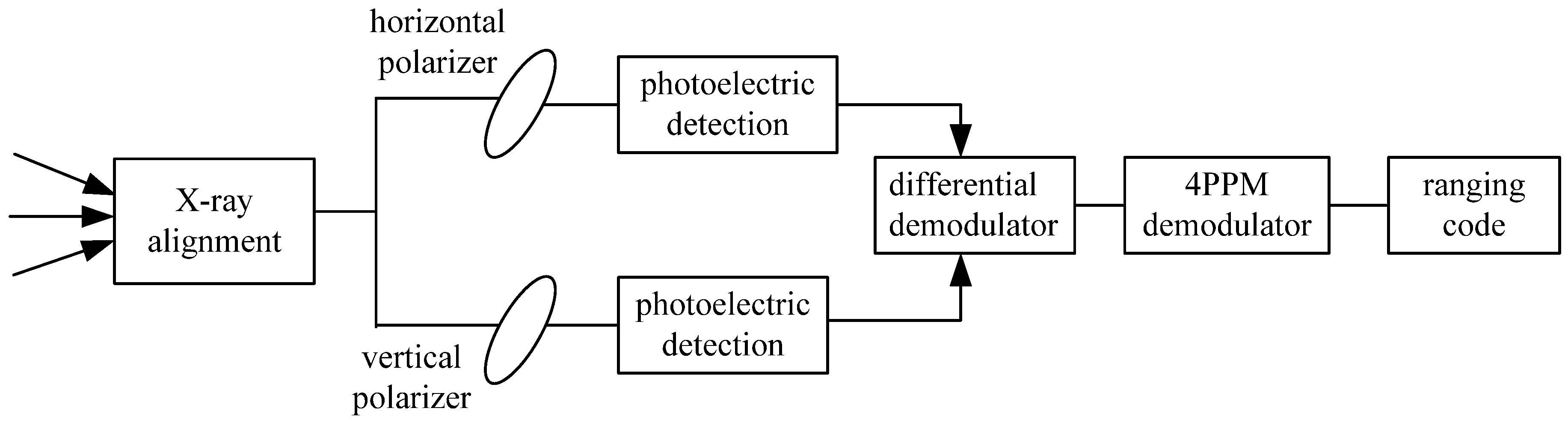
The X-ray ranging signal arrives at the slave station through propagation in the space channel. The block diagram of signal detection and demodulation is shown in Figure 4.

The light beam is collected and received by X-ray alignment devices. Then, the orthogonal linear polarized light can be divided into two independent channels [30,31,32]. The output intensity of the two signals is detected by a photoelectric detector. The left-hand and right-hand circular polarization states can be effectively detected, and then the ranging sequence information is demodulated.

The signal is received and demodulated at the slave station, and the demodulated signal is re-modulated and sent back to the master station, so as to eliminate the influence of link noise and signal attenuation and improve the ranging performance. Let $\left\{c_i^{\prime }\right\}$ denote the sequence of ranging obtained by demodulation of the master station, which can be denoted as

$$r^{\prime }(t)={\displaystyle \sum _i{c}_i^{\prime }g(t-i{T}_{\mathrm{C}}-{\tau }_{\mathrm{B}})}$$

(14)

where $\left\{c_i^{\prime }\right\}$ is the ranging code recovered from the main station and ${\tau }_{\mathrm{B}}$ is the bidirectional transmission time delay between the master and slave stations.

By pairing up the received sequence with the local sequence at the master station, we can obtain the two-way light travel time ${\tau }_{\mathrm{B}}$. Subsequently, the unidirectional range can be calculated by

$$d={\tau }_{\mathrm{B}}c/2$$

(15)

where $c$ is the speed of light.

2.2.3. Analysis of Ranging Error

Ranging error is an important index to measure the performance of the ranging system. Many factors will affect ranging performance, such as the Doppler effect, signal differential detection error, correlation error and so on [17]. This paper focuses on the influence of correlation errors on ranging performance.

As mentioned above, the $\{c_i^{\prime }\}$ should be correlated with each code component and its delay component of $\left\{c_i\right\}$ to obtain the bidirectional time delay ${\tau }_{\mathrm{B}}$. Because of the influence of noise, the time measurement error will occur when the signal is correlated. This paper takes the clock code component of the ranging code as an example to analyze. Because the clock code component is essentially a series of square waves, due to the effect of noise, its waveform will be deformed to some extent. The clock code component is modeled as [33].

$$r_{\mathrm{c}}(t)=\sqrt{P_{\mathrm{rc}}}\sin ({\omega }_{\mathrm{rc}}(t+\tau ))+n(t)$$

(16)

where $\sqrt{P_{\mathrm{rc}}}$ is the power of the clock code component, ${\omega }_{\mathrm{rc}}$ is the angular frequency, $n(t)$ is Gauss white noise and its power spectral density is $N_0/2$.

Suppose ${\gamma }_{1,0}$ is the result of the correlation between the clock code component and its in phase component, and ${\gamma }_{1,1}$ is the orthogonal component. They can be expressed as

$${\gamma }_{1,0}={\displaystyle \frac{4\sqrt{P_{\mathrm{rc}}}\cos ({\omega }_{\mathrm{rc}}\tau )T_{\mathrm{corr}}}{{\omega }_{\mathrm{rc}}{T}_{\mathrm{rc}}}}$$

(17)

$${\gamma }_{1,1}={\displaystyle \frac{4\sqrt{P_{\mathrm{rc}}}\sin ({\omega }_{\mathrm{rc}}\tau )T_{\mathrm{corr}}}{{\omega }_{\mathrm{rc}}{T}_{\mathrm{rc}}}}$$

(18)

Based on Equations (17) and (18), the time delay is calculated as

$$\tau ={\displaystyle \frac{1}{{\omega }_{\mathrm{rc}}}}\arctan ({\displaystyle \frac{{\gamma }_{1,1}}{{\gamma }_{1,0}}})$$

(19)

The variance of the time delay can be expressed as

$${\sigma }_{\tau }^2={\displaystyle \frac{1}{{\omega }_{\mathrm{rc}}^2({\gamma }_{1,0}^2+{\gamma }_{1,1}^2)}}{\displaystyle \frac{N_0}{2}}$$

(20)

Substituting Equations (17) and (18) into Equation (19), it can be rewritten as follows:

$${\sigma }_{\tau }^2={\displaystyle \frac{{\pi }^2{N}_0}{8{\omega }_{\mathrm{rc}}^2{P}_{\mathrm{rc}}{T}_{\mathrm{corr}}^2}}$$

(21)

The signal-to-noise ratio of the clock code component can be defined as

$$SN{R}_{\mathrm{rc}}={\displaystyle \frac{P_{\mathrm{rc}}}{N_0/2}}$$

(22)

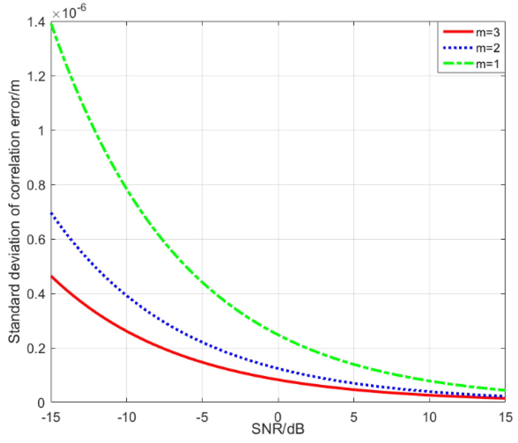
The standard deviation of the time delay can be expressed as

$${\sigma }_{\tau }={\displaystyle \frac{T_{\mathrm{rc}}}{4T_{\mathrm{corr}}\sqrt{SN{R}_{\mathrm{rc}}}}}$$

(23)

where $T_{\mathrm{rc}}=2\pi /{\omega }_{\mathrm{rc}}$ is the period of the clock code component.

3. ADDF Algorithm for State Estimation

As for the proposed method, both the pulsar timing observation and the range measurement are considered in the state determination of a spacecraft. In Section 2, the pulsar timing observation and the range measurement have been analyzed. Here, we would like to establish the measurement and orbit dynamic equation. Based on these equations, the ADDF filtering process can be established. ADDF is adopted as the iteration filter, which can estimate the process noise covariance matrix and adjust the noise covariance matrix depending on the level of the process noise to achieve a better state estimation.

3.1. Measurement Models

From the above section, we know that the high precision timing observation model of the spacecraft is shown in Equation (8). The TOA observation of the first pulsar is obtained as follows

$${\mathit{Y}}_1=g_1(\mathit{X},t)+v_1=\Delta t_1+v_1$$

(24)

where $\Delta t_1={\displaystyle \frac{{\mathit{n}}_1\cdot {\mathit{r}}_{\mathrm{SC}0}}{c}}+\Delta t_{\mathrm{SM}1}$ and $v_1$ is the first pulsar measurement noise, which is Gauss white noise with a mean value of zero, and its variance is determined by the pulsar measurement accuracy [1].

Similarly, The TOA observation of the second pulsar can be expressed

$${\mathit{Y}}_2=g_2(\mathit{X},t)+v_2=\Delta t_2+v_2$$

(25)

where $\Delta t_2={\displaystyle \frac{{\mathit{n}}_2\cdot {\mathit{r}}_{\mathrm{SC}0}}{c}}+\Delta t_{\mathrm{SM}2}$ and $v_2$ is the second pulsar measurement noise.

X-rays have good transmission characteristics in deep space. In this paper, the ranging information is used as the observation to improve the performance of XPNAV. The ranging observation model is given as follows

$${\mathit{Y}}_3=g_3(\mathit{X},t)+v_3=d+v_3$$

(26)

where $d={\tau }_{\mathrm{B}}c/2$, which is the range measured by XCOM based on PPM polarization modulation. $v_3$ is the ranging noise.

From what has been discussed above, it can be seen that the observation of XPNAV is

$$Y={[\begin{array}{ccc}{Y}_1& Y_2& Y_3\end{array}]}^{\mathrm{T}}={[\begin{array}{ccc}\Delta t_1& \Delta t_2& d\end{array}]}^{\mathrm{T}}+V$$

(27)

where $V={[\begin{array}{ccc}{v}_1& v_2& v_3\end{array}]}^{\mathrm{T}}$.

3.2. Orbital Dynamic Model

The state vector $X$ of the satellite consists of the position vector $r={[r_x r_y r_z]}^{\mathrm{T}}$ and the velocity vector $v={[v_x v_y v_z]}^{\mathrm{T}}$. The dynamic model of the nonlinear system can be expressed as [34].

$$\dot{X}=f\left(X\left(t\right),t\right)+w\left(t\right)$$

(28)

where $X={[r v]}^T={[x y z v_x v_y v_z]}^T$ and $w\left(t\right)$ is the state noise, also known as the process noise in the filter system. $f$ represents the nonlinear dynamic function of the state vector $X$ and it can be expressed as

$$f\left(X\left(t\right),t\right)=\left[\begin{array}{c}\dot{r}\\ \dot{v}\end{array}\right]=\left[\begin{array}{c}v\\ a\end{array}\right]$$

(29)

Integrating Equation (29) on both sides, the following equation is obtained

$$X(t)=X(t_0)+{\displaystyle {\int }_{t_0}^t}f(X(\tau ),\tau )d\tau$$

(30)

If the initial state of the satellite is known and the acceleration can be calculated, the position and velocity of the satellite can be solved [34,35].

3.3. ADDF Filtering Algorithm

Generally, discrete-time nonlinear equations can be expressed as [36,37].

$$\left\{\begin{array}{c}{x}_k=f\left(x_{k-1}\right)+w_k\\ y_k=g\left(x_k\right)+{\nu }_k\end{array}\right.$$

(31)

where $f\in R^{n\times 1}$ is the nonlinear dynamic function of the state vector $x(k)$ in this paper, $g\in R^{n\times 1}$ is the nonlinear observation function of $x(k)$, $w(k)\in R^{n\times 1}$ is the process noise of the system, $v(k)\in R^{n\times 1}$ is measurement noise and $w(k)$ and $v(k)$ are uncorrelated Gaussian white noise, so their mean and covariance matrices can be represented as

$$\left\{\begin{array}{c}E\left\{w\left(i\right)w^T\left(j\right)\right\}=Q\left(k\right){\delta }_{i,j}\\ E\left\{v\left(i\right)v^T\left(j\right)\right\}=R\left(k\right){\delta }_{i,j}\\ E\left\{w\left(i\right)v^T\left(j\right)\right\}=0\end{array}\right.$$

(32)

where ${\delta }_{i,j}$ is the Kronecker Delta function, $Q\left(k\right)$ is the covariance matrix of the process noise and $R\left(k\right)$ is the covariance matrix of the measurement noise.

The details of ADDF are presented in References [36,37] and the numerical simulation in Section 4.

4. Numerical Simulation Experiment

4.1. Simulation Conditions

The Satellite Tool Kit (STK) is a professional software for simulating the design, test, and operation of space missions [38]. Here, we use the STK to simulate accurate orbits. The GPS BIIA-10 and GPS BII-04 orbits are selected to verify the performance of the described method. GPS BIII-6 is used as the reference satellite. These parameters are listed in

Table 1. Initial orbital elements of the spacecraft.

Orbit	Eccentricity	Inclination/(°)	RAAN/(°)	Perigee/(°)	Mean Anomaly/(°)
GPS BIIA-10	0.015092	55.8352	313.291	280.004	78.2781
GPS BII-04	0.000847	54.5263	70.9472	321.537	38.3786
GPS BIII-6	0.000201	55.0862	169.042	286.417	71.4161

.

The parameters of the pulsars used in the simulation are listed in

Table 2. Pulsar parameters.

Pulsars	Right Ascension/(rad)	Declination/(rad)	Period/(s)	Flux Intensity/(ph/cm2·s)
B0531+21	1.4597	0.3493	3.34 × 10−2	6.41 × 10−2
B1821-24	4.8194	−0.4341	3.05 × 10−3	1.93 × 10−4
B1937+21	5.1472	0.3767	1.56 × 10−3	4.99 × 10−5

.

These pulsars are used for XPNAV in several studies and are considered as good candidates for XPNAV. The area of the X-ray detector is 1 ${\mathrm{m}}^2$ and the background noise is about 0.445 $\mathrm{ph}/{\mathrm{cm}}^2/\mathrm{s}$. If the position variance needs to be less than 500 m, the measurement time step for the pulsar observations is set up to 300 s, as was used in References [39,40]. The total filtering time is 300. The simulation parameters of the filter are described as follows.

The initial error is set to

$$\delta \mathit{X}(0)={\left[\begin{array}{cccccc}0.8 \mathrm{km}& 0.8 \mathrm{km}& 0.8 \mathrm{km}& 4 \mathrm{m}/\mathrm{s}& 4 \mathrm{m}/\mathrm{s}& 4 \mathrm{m}/\mathrm{s}\end{array}\right]}^T$$

The initial covariance matrix of the prediction error is set to

$$\mathit{P}=\mathrm{diag}\left(\right(0.08{ \mathrm{km})}^2, {(0.08 \mathrm{km})}^2, {(0.08 \mathrm{km})}^2, {(4 \mathrm{m}/\mathrm{s})}^2, {(4 \mathrm{m}/\mathrm{s})}^2, {(4 \mathrm{m}/\mathrm{s})}^2)$$

The covariance matrix of the process noise is set to

$$\mathit{Q}={\mathrm{diag}\left(\right(20 \mathrm{m})}^2, {(20 \mathrm{m})}^2, {(20 \mathrm{m})}^2, {(1 \mathrm{m}/\mathrm{s})}^2, {(1 \mathrm{m}/\mathrm{s})}^2, {(1 \mathrm{m}/\mathrm{s})}^2)$$

The timing observation noises of the three pulsars are calculated as 0.109 km, 0.325 km and 0.344 km. Thus, the covariance matrix of the measurement noise including the range measurement noise can be expressed as

$$R=\mathrm{diag}\left(\right(0.109{ \mathrm{km})}^2, {(0.325 \mathrm{km})}^2, {(0.0001 \mathrm{km})}^2)$$

4.2. Impact of Ranging Error on Filtering

In the simulation experiment, it is assumed that the emitter and detector between the master and slave stations have been accurately aligned and the state of circular polarization will not change when it propagates in space.

4.2.1. PPM Polarization Modulation Analysis

The theoretical analysis in Section 2.2.1 shows that the PPM circular polarization modulation can increase the capacity of the XCOM system. In this subsection, a simulation experiment will be carried out to analyze the influence of different modulation modes on ranging error. The order of m-sequence is set to be 6, the sampling frequency is $1 \mathrm{kHz}$, the carrier frequency is $20 \mathrm{Hz}$ and the slot duration is $T_{\mathrm{C}}=1 \times {10}^{-6} \mathrm{s}$. The polarizing transmittance is set to 50% [41]. The comparison of ranging errors under different modulation modes is shown in Figure 5.

As can be seen from Figure 5, when the SNR is −15 dB, the mean ranging error with PPM polarization modulation is about 21 m, while the mean error of PPM is 32 m. As the SNR increases, the ranging error goes down. When SNR is greater than 0 dB, a relatively stable ranging error of 16 m is obtained. As we expected, polarization modulation reduces the influence of noise on the ranging signal, and the new method can increase the ranging accuracy.

4.2.2. Correlation Error Analysis

Because of the influence of noise on the signal, the time measurement error will emerge when the signal is correlated, and then the accuracy of ranging will be reduced. In the simulation, the Monte Carlo method is used to analyze the variance of the ranging error under different SNR levels. Let L be the length of the T4B code and the correlation time be set to an integer multiple of the ranging sequence, that is, $T_{\mathrm{corr}}=mL{T}_{\mathrm{C}} (m=1,2,3\dots )$. The slot duration is $T_{\mathrm{C}}=1\times {10}^{-6} \mathrm{s}$. The standard deviation of the time measurement error caused by the correlation of the ranging signal is shown in Figure 6. The abscissa represents the SNR of the ranging clock code component and the ordinate represents the standard deviation of the time measurement error caused by the correlation process. We can see that as the SNR increases, the standard deviation goes down. When the SNR is 0 dB, the standard deviation of the correlation error is about $1\times {10}^{-7} \mathrm{m}$. The improvement of SNR can improve the ranging performance. In addition, it can be found that the longer the correlation time is, the smaller the measurement error is, but the greater the amount of calculation is, and that the real-time performance of signal detection will also be affected.

4.2.3. SNR of Ranging Signal on Filtering

The ranging as the extra observation is utilized to augment XPNAV. The accuracy of the range measurement will have an effect on the filtering performance. In this subsection, the impact of the SNR of the ranging signal on the position and velocity estimation will be analyzed.

In the simulation, the initial conditions are as follows: (1) GPS BIIA-10 in Table 1 is used as the orbit. (2) The SNR of the ranging signal is set to be −15 dB to 5 dB. (3) ADDF is selected to estimate the state of the spacecraft.

The statistical comparison results in different cases are shown in

Table 3. Influence of SNR on position and velocity estimation.

SNR (dB)	Position Estimation Error (km)		Velocity Estimation Error (m/s)
	Mean	StdDev	Mean	StdDev
−15	0.6146	0.4546	0.5650	0.3862
−10	0.5811	0.4857	0.5872	0.4091
−5	0.5663	0.4148	0.5499	0.3594
0	0.5764	0.4148	0.5490	0.3441
5	0.5571	0.3912	0.5206	0.3449

StdDev: standard deviation.

for clarity.

From Table 3, when the SNR changes from −15 dB to 5 dB, the ranging error only fluctuates about 6 m and the standard deviation of the position estimation error fluctuates by 0.0945 km, while the velocity estimation error by 0.065 m/s. It can be seen that within a certain range of SNR, the SNR of the ranging signal has less influence on the system state estimation. This is because the XPNAV system noise includes ranging noise and pulsar observation noise. On the one hand, the observation noise of the pulsar signal is high, which plays a major role in the estimation of system performance. On the other hand, the X-ray ranging measurement is good in terms of performance. Such a small jitter can be neglected in deep space and the long-distance environment. It can be concluded that when the SNR varies from −15 dB to 5 dB, its effect on the position and velocity estimation error of the spacecraft can be ignored.

4.3. State Estimation Based on ADDF

To demonstrate the performance of the proposed method, two cases are designed. Case 1 uses the timing observation. Case 2 uses the timing and ranging observations simultaneously. Both cases use an ADDF as the filter algorithm. The orbit used in the simulation is GPS BIIA-10, whose parameters have been given in Table 1. For Case 1, all three pulsars listed in Table 2 are used for the state estimation. For Case 2, the first two pulsars listed in Table 2 are utilized to achieve the pulsar timing observation. The SNR of the ranging signal is set to be 0 dB and the slot duration $T_{\mathrm{C}}=1\times {10}^{-6} \mathrm{s}$. After 100 Monte Carlo simulations, the mean error and standard deviation error of the spacecraft’s state are obtained to evaluate the performance.

The results are shown in Figure 7. The abscissa corresponds to the number of iterations of the filtering process, and the ordinate corresponds to the position or velocity estimation error or the cumulative error with the different methods. The term “Timing” denotes the traditional timing observation. The term “Timing and Ranging” denotes that the timing and the ranging observation information fusion algorithm is used. Figure 7a,b illustrate that if only the timing observation is used, the result has the maximum estimation error. In comparison, the filter result using the timing together with the ranging measurement is better under the simulation condition.

The statistical data are shown in the

Table 4. Estimation errors under different observation models.

Filters	Observations	Position Estimation Error (km)		Velocity Estimation Error (m/s)
		Mean	StdDev	Mean	StdDev
ADDF	Timing	0.9883	0.5780	1.1113	0.4802
ADDF	Timing and Ranging	0.5829	0.4196	0.5241	0.3739
UKF	Timing and Ranging	0.6647	0.5687	0.5493	0.4742

StdDev: standard deviation.

. When the timing and the ranging observations are both used, the standard deviation of position error can decrease from 0.5780 km to 0.4196 km, and the velocity can decrease from 0.4802 m/s to 0.3739 m/s. The results show that the performance of the proposed method is improved by 27% in position and 22% in velocity compared with the traditional method. It is verified that the range measurement can improve the navigation performance.

To investigate the performance of the ADDF, the comparison between ADDF and UKF is shown in Figure 8.

In Figure 8, the abscissa corresponds to the iteration times of the filtering process and ordinate denotes the position or velocity estimation error. The term “ADDF” and “UKF” indicate that the adaptive divided difference filter or the unscented Kalman filter is used to estimate the satellite state in the simulation. From Figure 8, it can be seen that the performance of ADDF is better than UKF. The statistical data are shown in Table 4. The standard deviation of the position error can decrease from 0.5687 km to 0.4196 km and the velocity can decrease from 0.4742 m/s to 0.3739 m/s. The performance of ADDF is improved by 26% in position and 21% in velocity compared with UKF. The ADDF filter has the best navigation precision by adjusting the covariance matrix of the process noise. This characteristic of the ADDF filter will be extremely valuable in a situation where the process noise is hard to calculate in XPNAV.

4.4. Influence of Different Orbits on Filtering

To verify the applicability of the proposed XPNAV differential enhancement algorithm, the GPS BII-04 is selected for the simulation.

As can be seen from

Table 5. State estimation in different orbits.

Orbit	Position Estimation Error (km)		Velocity Estimation Error (m/s)
	Mean	StdDev	Mean	StdDev
GPS BIIA-10	0.5829	0.4196	0.5241	0.3739
GPS BII-04	0.6159	0.4226	0.5574	0.3694

StdDev: standard deviation.

, the position and velocity estimation error of the spacecraft are very close under the two orbits, that is, the algorithm has consistency and universal applicability.

5. Conclusions

In this paper, we address an augmentation XPNAV method based on ranging and difference timing observations simultaneously. The position measurement error of the reference satellite is used as a correction to improve the state estimation accuracy of the spacecraft. The range between the spacecraft and the reference satellite based on XCOM has a higher accuracy. With the assistance of ranging observation, the number of pulsars needed to be observed is reduced, and the positioning accuracy of the spacecraft is improved. The simulation results indicate that the multi-information fusion algorithm based on ADDF can improve the position estimation accuracy by 27% and the velocity estimation accuracy by 22% compared with the traditional timing observation. Experiments also demonstrate that PPM polarization modulation can expand XCOM capacity and effectively reduce ranging error. The method proposed in this paper realizes the high-precision autonomous navigation of spacecraft, which can be extended to the whole solar system. With the increasing demand for autonomous navigation and the large volume of data transmission, simultaneous communication and navigation could provide a potential option for future deep space explorations.

References

1. Sheikh, S.I. The Use of Variable Celestial X-Ray Sources for Spacecraft Navigation. Ph.D. Thesis, University of Maryland, College Park, MD, USA, 2005. [Google Scholar]
2. Li, J.X.; Ke, X.Z.; Zhao, B.S. A new time-domain estimation method for period of pulsars. Acta Phys. Sin. 2012, 61, 069701. [Google Scholar]
3. Zhang, H.; Xu, L.P.; Xie, Q. X-ray pulsar weak signal detection based on Bayesian estimation. Acta Phys. Sin. 2011, 60, 049701. [Google Scholar] [CrossRef]
4. Fang, H.Y.; Liu, B.; Li, X.P. Time delay estimation method of X-ray pulsar observed profile based on the optimal frequency band. Acta Phys. Sin. 2016, 65, 119701. [Google Scholar] [CrossRef]
5. Kang, Z.W.; Xu, X.M.; Liu, J.; Li, N. Doppler velocity measurement based on double measurement model and its integrated navigation. J. Astronaut. 2017, 38, 964–970. [Google Scholar] [CrossRef]
6. Liu, J.; Fang, J.C.; Yang, Z.H. X-ray pulsar/Doppler difference integrated navigation for deep space exploration with unstable solar spectrum. Aerosp. Sci. Technol. 2015, 41, 144–150. [Google Scholar] [CrossRef]
7. Rinauro, S.; Colonnese, S.; Scarano, G. Fast near-maximum likelihood phase estimation of X-ray pulsars. Signal Process. 2013, 93, 326–331. [Google Scholar] [CrossRef]
8. Su, Z.; Xu, Q.B.; Wang, X.L.; Wang, Y. Pulsar integrated pulse profile time delay measurement based on two-level cross ambiguity function. Space Electron. Technol. 2016, 5, 14–20. [Google Scholar]
9. Shannon, R.M.; Oslowski, S.; Dai, S. Limitations in timing precision due to single-pulse shape variability in millisecond pulsars. Mon. Not. R. Astron. Soc. 2014, 39, 1463–1481. [Google Scholar] [CrossRef]
10. Yang, B.; Hu, S.M.; Sun, H. Integrated single X-ray pulsar and starlight navigation based on virtual observation value. J. Beijing Univ. Aeronaut. Astronaut. 2016, 42, 1107–1115. [Google Scholar]
11. Jiao, R.; Xu, L.P.; Zhang, H.; Li, C. Orbit determination using incremental phase and TDOA of X-ray pulsar. Front. Inf. Technol. Electron. Eng. 2016, 17, 543–552. [Google Scholar] [CrossRef]
12. Zhang, H.; Jiao, R.; Xu, L.P. Orbit determination using pulsar timing data and orientation vector. J. Navig. 2019, 72, 155–175. [Google Scholar] [CrossRef]
13. Hemmati, H. Deep Space Optical Communications; Simplified Chinese translation edition; Tsinghua University Press: Beijing, China, 2006; p. 73. [Google Scholar]
14. Mitchell, J.W. Pulsar Navigation and X-ray Communication Demonstrations with the NICER Payload on the ISS. In Proceedings of the 1st Annual ISS Research and Development Conference, Denver, CO, USA, 25–28 June 2013. [Google Scholar]
15. Zhao, B.S.; Wu, C.X.; Sheng, L.Z.; Liu, Y.A. Next Generation of Space Wireless Communication Technology Based on X-ray. Acta Photonica Sin. 2013, 42, 801–804. [Google Scholar] [CrossRef]
16. Chen, X.; Qiu, J.; Wang, T.; Li, M. Onboard mission planning for autonomous avoidance of spacecraft subject to various orbital threats: An SMT-based approach. IEEE Trans. Aerosp. Electron. Syst. 2024, 1–12. [Google Scholar] [CrossRef]
17. Li, Y.; Su, T.; Shi, F. Bit error rate analysis of the spatial X-ray communication system. Infrared Laser Eng. 2018, 47, 622001. [Google Scholar] [CrossRef]
18. Song, S.B.; Xu, L.P.; Zhang, H.; Bai, Y.J. Novel X-ray communication based XNAV augmentation method using X-ray detector. Sensors 2015, 15, 22325–22342. [Google Scholar] [CrossRef] [PubMed]
19. Jenner, L. NASA Set to Demonstrate X-Ray Communications in Space. 2019. Available online: https://www.nasa.gov/feature/goddard/2019/nasa-set-to-demonstrate-x-ray-communications-in-space (accessed on 2 December 2024).
20. Deng, N.; Zhao, B.; Sheng, L.; Yan, Q.; Yan, H.; Liu, D. A space audio communication system based on X-ray. Acta Phys. Sin. 2013, 62, 060705. [Google Scholar] [CrossRef]
21. Wang, R.; Xue, F.; Xue, Y.; Lin, J.; Li, N. Performance improving method of X-ray communication system based on QAM modulation. Laser Optoelectron. Progress 2019, 6, 251–256. [Google Scholar]
22. Ke, X.Z.; Yin, Z.Y.; Yang, L.H. Light polarization modulation with PPM and its key technique in atmospheric laser communication. Semicond. Optoelectron. 2007, 28, 553–560. [Google Scholar] [CrossRef]
23. Song, S.; Xu, L.; Zhang, H.; Gao, N.; Shen, Y. A novel X-ray circularly polarized ranging method. Chin. Phys. B 2015, 24, 057201. [Google Scholar] [CrossRef]
24. Jiao, R.; Xu, L.P.; Zhang, H.; Li, C. Augmentation method of XPNAV in Mars Orbit based on Phobos and Deimos observations. Adv. Space Res. 2016, 58, 1864–1878. [Google Scholar]
25. Taylor, J.H. Pulsar timing and relativistic gravity. Philos. Trans. R. Soc. A Math. Phys. Eng. Sci. 1992, 341, 117–134. [Google Scholar] [CrossRef]
26. Ma, J.; Jiang, Y.; Yu, S. Packet error rate analysis of OOK, DPIM and PPM modulation schemes for ground-to-satellite optical communications. Opt. Commun. 2010, 283, 237–242. [Google Scholar] [CrossRef]
27. Black, J.K.; Baker, R.G.; Deines-Jones, P.; Hill, J.E.; Jahoda, K. X-ray polarimetry with a micropattern tpc. Nuclear Instrum. Methods Phys. Res. Section A Accel. Spectrom. Detect. Assoc. Equip. 2007, 581, 755–760. [Google Scholar] [CrossRef]
28. Schaefers, F. Multilayer-based soft X-ray polarimetry. Opt. Precis. Eng. 2007, 15, 1850–1861. [Google Scholar]
29. Yahnke, C.J.; Srajer, G.; Haeffner, D.R.; Mills, D.; Assoufid, L. Germanium X-ray phase plates for the production of circularly polarized X-rays. Nuclear Instrum. Methods Phys. Res. Sect. A Accel. Spectrom. Detect. Assoc. Equip. 1994, 347, 128–133. [Google Scholar] [CrossRef]
30. Li, L.; Mei, Z.; Deng, L.; Lü, Z.; Liu, J.; Sun, J.; Sun, Y.; Zhou, H.; Zuo, F. Assembly error analysis and in-orbit verification of grazing incidence focusing X-ray pulsar telescope. J. Mech. Eng. 2018, 54, 49–60. [Google Scholar] [CrossRef]
31. Liu, D.; Qiang, P.; Li, L.; Su, T.; Sheng, L.; Liu, Y.; Zhao, B. X-ray focusing optics and its application in X-ray communication system. Acta Phys. Sin. 2016, 65, 010703. [Google Scholar]
32. Shi, Y.; Xi, T.; Xin, Y.; Chen, J.; Deng, L.; Lv, Z.; Mei, Z. The energy response calibration of FXPT. Aerosp. Control Appl. 2018, 44, 34–39. [Google Scholar]
33. CCSDS. Pseudo-Noise (PN) Ranging Systems; Consultative Committee for Space Data Systems (CCSDS): Washington, DC, USA, 2014. [Google Scholar]
34. Qiao, L.; Liu, J.; Zheng, G.; Xiong, Z. Augmentation of XNAV system to an ultraviolet sensor-based satellite navigation system. IEEE J. Sel. Top. Signal Process. 2009, 3, 777–785. [Google Scholar] [CrossRef]
35. Chen, X.; Wang, T.; Qiu, J.; Feng, J. Mission planning on autonomous avoidance for spacecraft confronting orbital debris. IEEE Trans. Aerosp. Electron. Syst. 2024, 1–11. [Google Scholar] [CrossRef]
36. Dey, A.; Sadhu, S.; Ghoshal, T.K. Adaptive divided difference filter for nonlinear systems with unknown noise. In Proceedings of the 2014 International Conference on Control, Instrumentation, Energy and Communication (CIEC), Calcutta, India, 31 January–2 February 2014. [Google Scholar]
37. Subrahmanya, N.; Shin, Y.C. Adaptive divided difference filtering for simultaneous state and parameter estimation. Automatica 2009, 45, 1686–1693. [Google Scholar] [CrossRef]
38. McCamish, S.B.; Ciarcià, M.; Marcello, R. Simulations of Multiple Spacecraft Maneuvering with MATLAB/Simulink and Satellite Tool Kit. J. Aerosp. Inf. Syst. 2013, 10, 348–358. [Google Scholar] [CrossRef]
39. Sheikh, S.I.; Pines, D.J.; Ray, P.S. Spacecraft navigation using X-ray pulsars. Guid. Control. Dyn. 2006, 29, 49–63. [Google Scholar] [CrossRef]
40. Sheikh, S.I.; Hanson, J.E.; Graven, P.H. Spacecraft navigation and timing using X-ray pulsars. Navigation 2011, 58, 165–186. [Google Scholar] [CrossRef]
41. Dwyer, J.R. Polarization of X-rays and Gamma-Rays produced by Thunderstorms and Lightning. In Proceedings of the AGU Fall Meeting, San Francisco, CA, USA, 15–19 December 2014. AGU Fall Meeting Abstracts. [Google Scholar]
Figure 1. Scheme of differential enhancement for pulsar navigation.
Aerospace 12 00113 g001
Figure 2. The 4PPM circular polarization modulation pulse diagram.
Aerospace 12 00113 g002
Figure 3. Block diagram of ranging signal modulation.
Aerospace 12 00113 g003
Figure 4. Block diagram of ranging signal detection and demodulation.
Aerospace 12 00113 g004
Figure 5. Comparison of ranging errors under different modulation modes.
Aerospace 12 00113 g005
Figure 6. Standard deviation of correlation error.
Aerospace 12 00113 g006
Figure 7. Navigation precision of spacecraft with different methods.
Aerospace 12 00113 g007
Figure 8. Position and velocity estimation error of ADDF and UKF.
Aerospace 12 00113 g008