Article

GAT-BiGRU-TPA City Pair 4D Trajectory Prediction Model Based on Spatio-Temporal Graph Neural Network

1
School of Emergency Management and Safety Engineering, North China University of Science and Technology, Tangshan 063000, China
2
Tangshan Key Laboratory of Air—Ground Intelligent Transportation, Tangshan 063000, China
*
Author to whom correspondence should be addressed.
Aerospace 2025, 12(11), 999; https://doi.org/10.3390/aerospace12110999 (registering DOI)
Submission received: 23 August 2025 / Revised: 30 October 2025 / Accepted: 5 November 2025 / Published: 8 November 2025
(This article belongs to the Section Air Traffic and Transportation)

Abstract

With the rapid expansion of the civil aviation industry, the surge in flight numbers has led to increasingly pronounced issues of air route congestion and flight conflicts. 4D trajectory prediction, by dynamically adjusting aircraft paths in real time, can prevent air route collisions, alleviate air traffic pressure, and ensure flight safety. Therefore, this paper proposes a combined model—GAT-BiGRU-TPA—based on the Spatio-Temporal Graph Neural Network (STGNN) framework to achieve refined 4D trajectory prediction. This model integrates Graph Attention Networks (GAT) to extract multidimensional spatial features, Bidirectional Gated Recurrent Units (BiGRU) to capture temporal dependencies, and incorporates a Temporal Pattern Attention (TPA) mechanism to emphasize learning critical temporal patterns. This enables the extraction of key information and the deep fusion of spatio-temporal features. Experiments were conducted using real trajectory data, employing a grid search to optimize the observation window size and label length. Results demonstrate that under optimal model parameters (observation window: 30, labels: 4), the proposed model achieves a 45.72% reduction in mean Root Mean Square Error (RMSE) and a 43.40% decrease in Mean Absolute Error (MAE) across longitude, latitude, and altitude compared to the optimal baseline BiLSTM model. Prediction accuracy significantly outperforms multiple mainstream benchmark models. In summary, the proposed GAT-BiGRU-TPA model demonstrates superior accuracy in 4D trajectory prediction, providing an effective approach for refined trajectory management in complex airspace environments.

1. Introduction

In recent years, with the rapid development of the civil aviation industry, the scale of airlines has continued to expand, the number of flights has steadily increased, and air traffic volume has grown rapidly. This has led to issues such as air route congestion and conflicts, while the risk of mid-air collisions has also increased. Traditional air traffic management models are increasingly unable to meet the growing demands of aviation transportation. To address these issues, the International Civil Aviation Organization (ICAO) has proposed the concept of Trajectory-Based Operations (TBO) [1]. This concept leverages four-dimensional trajectory prediction technology to forecast aircraft trajectories accurately, coordinate airspace resources across temporal and spatial dimensions, optimize flight operations, achieve precise airspace management, and ensure flight safety.
Currently, trajectory prediction methods can be categorized into state estimation methods, dynamic methods, and machine learning methods [2]. To achieve estimation propagation, state estimation methods establish motion equations based solely on the aircraft’s position, speed, acceleration, and other attributes. This approach is solely applicable for short-term forecasting. Dynamic methods analyze the forces acting on the plane. Still, most are implemented under ideal conditions and are easily constrained by aircraft performance, aircraft state, and environmental conditions, making it challenging to predict trajectories under real-world conditions.
With the increasing development of machine learning, a growing number of scholars are gradually applying it to trajectory prediction. LAN MA et al. [3] proposed a novel 4D trajectory prediction hybrid model combining convolutional neural networks (CNN) and long short-term memory (LSTM). They employed one-dimensional convolutional layers to capture features in the spatial domain from trajectory data and leveraged LSTM networks to learn temporal dependencies. This spatio-temporal integrated framework subsequently improved the precision of trajectory forecasting. Deepudev Sahadevan et al. [4] proposed a bidirectional long short-term memory (Bi-LSTM) neural network model. By leveraging the bidirectional structure of BiLSTM, the model can understand both forward and backwards dependencies in trajectory time-series data, thereby improving the accuracy of trajectory prediction. Peiyan Jia et al. [5] presented a 4D trajectory prediction model based on an LSTM encoder augmented with an attention mechanism. The LSTM captured the temporal characteristics of the trajectories, while the attention module weighted the sequential features, leading to a significant improvement in forecasting accuracy. Long short-term memory (LSTM) and its variants have been widely used in current research. Still, they suffer from gradient vanishing and gradient explosion issues due to the iterative output of cumulative errors. To address this problem, Aofeng Luo et al. [6] proposed a long-term trajectory prediction model based on an improved Transformer, utilizing self-attention mechanisms to extract time-series features from historical trajectory data, and introducing a trajectory stabilization module to address long-term prediction scenarios, ensuring the smoothness of time-series data and achieving better predictability. Shi Qingyan et al. [7] developed the GTA-Seq2Seq framework for multi-step 4D trajectory prediction. This model architecturally integrates a sequence-to-sequence (Seq2Seq) structure with Gated Recurrent Units (GRUs), a Temporal Convolutional Network (TCN), and a Temporal Pattern Attention (TPA) mechanism. The model achieves high-precision multi-step trajectory prediction by extracting the temporal dependency and spatial features from trajectory data and combining them with TPA. Hua Li et al. [8] utilized the sine chaotic map enhanced sparrow search algorithm (Sine-SSA) to optimize the threshold parameters of the BP neural network to enhance its global search capability. After integrating the optimal weight threshold obtained by Sine-SSA into the BP, they performed trajectory prediction based on aircraft 4D trajectory data. Zhao Yuandi et al. [9] proposed a deep learning-based multi-task learning method for 4D trajectory multi-step prediction, achieving fast and high-precision 4D trajectory prediction. During the process of predicting 4D trajectory, numerous unpredictable factors may influence trajectories, including weather conditions, aircraft performance, and conflicts among multiple aircraft. Consequently, optimization of multi-agent routing and landing problems must be considered. Yong Lu et al. [10] addressed the challenge of optimizing landing windows for manned aircraft within low-altitude intelligent transport systems. They proposed a Quantum-Enhanced Whale Optimization Algorithm (QEWOA) that significantly enhances global search capabilities, optimization accuracy, and convergence speed. This approach introduces a novel high-dimensional real-time optimization methodology for 4D trajectory prediction. Yujiao Hu et al. [11] addressed multi-agent routing challenges by developing RouteMaker, an approach that integrates Role-Interaction-based Graph Neural Networks (RIGNN) with deep reinforcement learning. Through training on small-scale problems, it achieves rapid, high-quality solutions for large-scale and real-world scenarios, providing a scalable, generalizable intelligent decision-making framework and algorithmic foundation for 4D trajectory prediction.
The aforementioned machine learning-based trajectory prediction methods, whilst mitigating the vanishing or exploding gradients caused by cumulative errors in traditional approaches to some extent, still exhibit shortcomings in the refined extraction of multidimensional spatial features, the deep integration of spatio-temporal characteristics, and the focused attention on critical temporal patterns within trajectories. Concurrently, prediction errors for multi-step outputs progressively increase with the number of steps. In light of this, this paper proposes a four-dimensional trajectory prediction model with multi-variable input-output, based on the STGNN framework and integrating GAT, BiGRU, and TPA. GAT precisely extracts multidimensional spatial features from trajectory data, addressing the limited spatial feature capture in existing models. BiGRU is employed to extract temporal features, promoting spatio-temporal integration. TPA is integrated to highlight significant temporal patterns in trajectory data, compensating for the limited focus of existing models on critical sequential information. Furthermore, a grid search optimizes observation windows and labels to minimize prediction errors in multi-step outputs. This approach enhances adaptability to complex trajectory prediction scenarios, thereby partially overcoming limitations in existing research.

2. Model Framework Construction

Trajectory data is a time series with multi-dimensional features, including temporal and spatial dimensions. Interdependent spatial information exists among the spatial dimensions of longitude, latitude, and altitude. During the aircraft operation phase, as altitude changes, both longitude and latitude also change accordingly, and this spatial information is highly correlated with the temporal trend, highlighting the close connection between spatial and temporal dimensions. To effectively capture the spatio-temporal dependencies inherent in aircraft trajectory data, this paper introduces a framework based on Spatio-Temporal Graph Neural Networks (STGNN). By synthesizing graph neural networks with advanced temporal learning, the proposed approach formulates a novel GAT-BiGRU-TPA model for 4D trajectory prediction. The following section details the specific components of each module in the model.
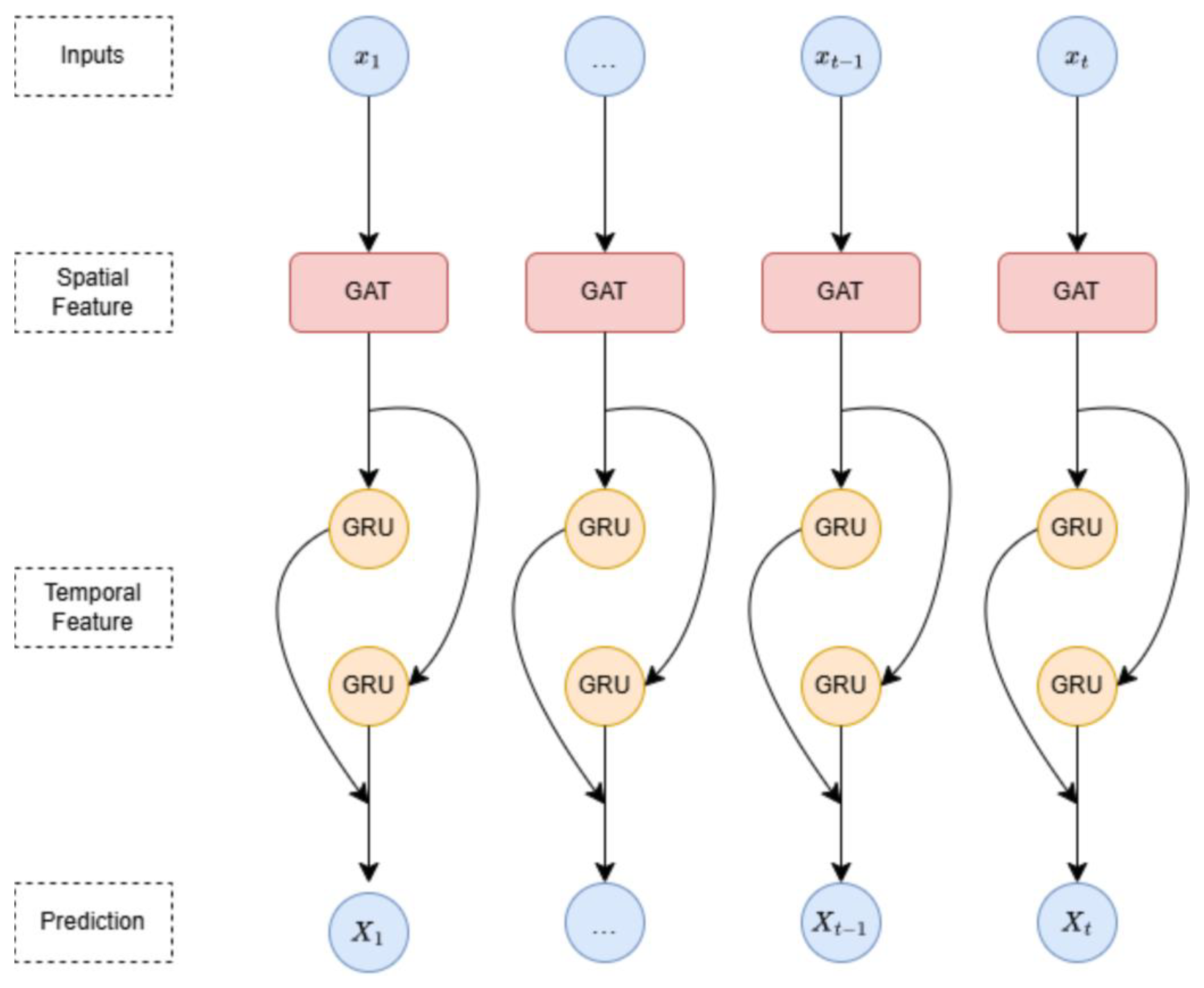
The first part of the model is the historical input data, which includes historical trajectory data with six features: time, altitude, speed, heading, longitude, and latitude. The second part of the model is the data preprocessing module, which cleans, detects, and handles outliers in the input historical trajectory data, performs data resampling, and normalizes the data to generate high-quality trajectory data for spatio-temporal graph construction. The third part of the model is the spatio-temporal feature fusion module, which inputs the trajectory data processed through data pre-processing into a graph attention network (GAT) to extract spatial features and utilize a graph attention network to capture and use the relationships between variables. Then, input the temporal sequence data into a temporal learning network (BiGRU) to capture the past and future dependencies of the temporal sequence data, and extract important temporal patterns from the temporal sequence data using TPA. The spatial and temporal feature extraction modules are layered sequentially to construct a comprehensive spatio-temporal integrated neural network. The fourth part of the model is the training and prediction module, which takes the fused spatio-temporal features as input and passes them through a GRU network. This network then converts these features into target prediction features using a fully connected layer, enabling fine-grained prediction of four-dimensional trajectories. The final part outputs the predicted time, altitude, longitude, and latitude data. The model framework is shown in Figure 1.

3. Data Processing

3.1. Data Sources

A standard flight within traditional civil aviation is divided into seven distinct operational phases: takeoff, climb, departure, cruise, arrival, approach, and landing. The original trajectory data consists of discrete points, which may contain missing, unreasonable, or duplicate data points. The data in this study is sourced from the VarFlight website’s Automatic Dependent Surveillance-Broadcast (ADS-B) system. ADS-B is a satellite-based air traffic management surveillance technology that transmits aircraft status information (such as latitude, longitude, altitude, airspeed, and heading) via a data link to other authorized users for surveillance and flight monitoring.
Taking into account the differences in the management of different types of aircraft during flight, the full trajectory data of China Eastern Airlines’ MU5102, MU5104, MU5106, MU5108, MU5112, MU5114, MU5120, MU5122, and MU5124 flights from Beijing Capital International Airport to Shanghai Hongqiao International Airport were selected. The time span was selected from 1 March 2025 to 31 May 2025, with a total of 521,482 historical trajectory data and 788 historical flights. Multiple trajectory points of a flight contain the following features, as shown in Table 1. The three-dimensional visualization of the original trajectory data is shown in Figure 2.

3.2. Data Preprocessing

3.2.1. Outlier Detection and Processing

The original trajectory data contains some outliers significantly different from other data points in the dataset. These outliers may significantly affect the experiment’s predictive accuracy. A neural network-based algorithm, Autoencoder [12], is used for outlier detection of data.
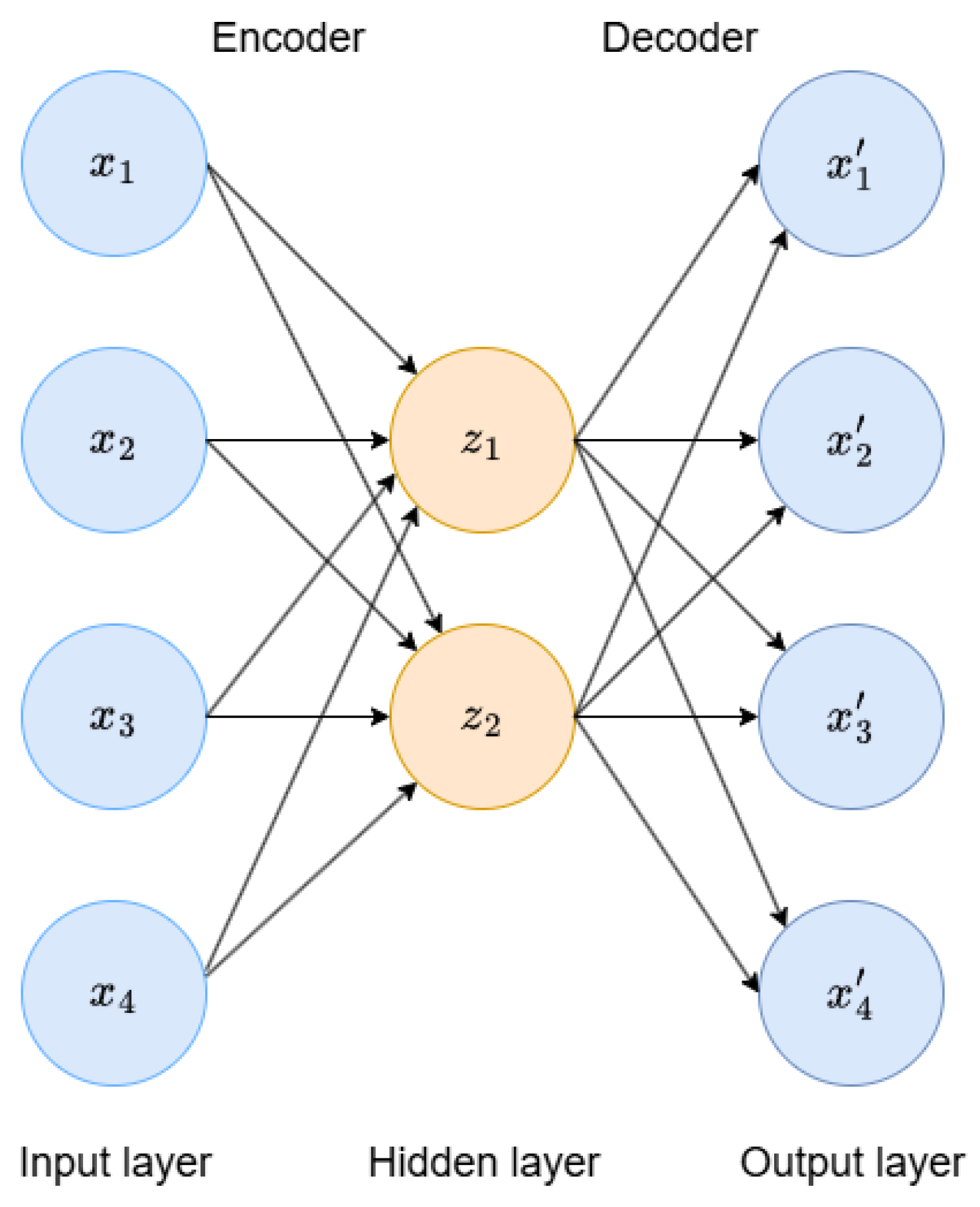
An autoencoder is an unsupervised method for data dimension reduction and feature representation, consisting of an encoder and a decoder. The structure of an autoencoder is shown in Figure 3:
The layer containing the sample x is the input layer, and the intermediate hidden layers represent the encoding of x. The calculation method is as follows:
z = f W 1 x + b 1
The output of the autoencoder is the reconstructed data:
x = f W 2 z + b 2
In Formulas (1) and (2), W 1 , W 2 , b 1 , and b 2 are the parameters of the autoencoder network, obtained through gradient descent training.
As shown in Figure 3, in the encoder part, the input data (altitude, speed, longitude, latitude, and heading) are linearly transformed into 16 dimensions, input into the Input layer, and the linear transformation results are nonlinearized using the ReLU activation function. Then, the 16 dimensions are further linearly transformed into 8 dimensions, input into the Hidden layer, and the ReLU activation function is applied again to achieve dimension reduction. In the decoder part, the 8-dimensional data from the Hidden layer is linearly transformed back to 16 dimensions, and a ReLU activation function is applied. Then the data is linearly transformed back to a 5-dimensional feature space to reconstruct the data. The mean squared error (MSE) is used as the loss function. Through multiple rounds of training, the autoencoder can reconstruct standard samples well. The reconstruction error of each sample is calculated, and the 95th percentile is used as the threshold to mark samples exceeding this threshold as outliers. For the selected outliers, we apply the moving average smoothing method [13]. We set a window size of 5 for the same-day data and replace outliers with the average of surrounding data points to generate a smoothed feature column, thereby improving data quality and the accuracy of subsequent model predictions.

3.2.2. Data Resampling

In real-world collected trajectory data, the duration between successive points varies. Effective trajectory forecasting often depends on equally spaced time-series data for optimal performance. The altitude, longitude, and latitude features relative to time are processed using cubic spline interpolation [14], i.e., resampling the time series data into a time series with a time interval of 10 s, and constructing the cubic spline interpolation function as shown in Formula (3):
S i x = a i + b i x x i + c i x x i 2 + d i x x i 3
In Formula (3), x x i , x i + 1 , i = 0 , 1 , 2 , , n 1 , a i , b i , c i , and d i are the coefficients to be determined.
Construct a cubic spline interpolation function in two dimensions. The first dimension is the time dimension, where the original data’s time series is resampled to a 10 s interval. The time dimension is the independent variable that determines the interpolation points in the spatial dimension. The second dimension is the spatial dimension (x, y, z), which constructs a cubic spline interpolation function S i x for each spatial dimension. The time points in the time series are used as nodes x i = t i (i = 0, 1, 2, …, n), and use the corresponding x-coordinate values as y i = x i to determine the cubic polynomial S i t for each interval t i , t i + 1 , where t is the time variable. By ensuring that the interpolation conditions are satisfied at the original data points and satisfying the continuity conditions for the first and second derivatives at the internal nodes, a system of equations is established to determine the coefficients a i ,   b i ,   c i ,   d i for each interval. Based on the above cubic spline interpolation process, starting from the initial time t i of the original time series, a new time point is generated every 10 s until the last original time point t n .
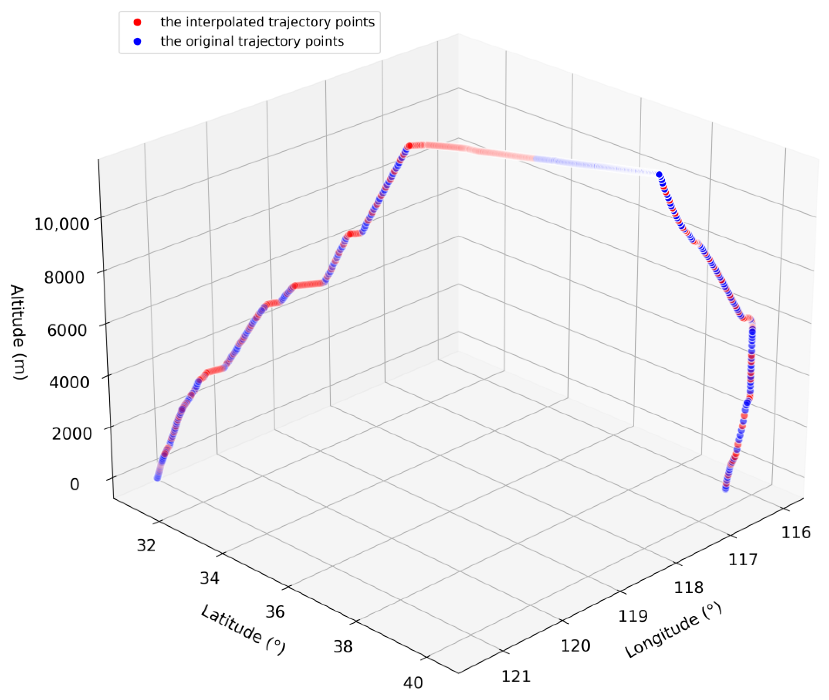
Following outlier detection and processing, cubic spline interpolation was used to resample the trajectory data to high-quality 10 s intervals. A visualization of a single processed full trajectory is shown in Figure 4. The blue trajectory points represent the original trajectory, while the red points denote the interpolated trajectory. Evidently, the reconstructed trajectory effectively addresses trajectory outliers and temporal intervals.

3.2.3. Processing of the Time Column

To better capture and utilize the time-dependent relationships in the time series, the time dimension of the trajectory sequence was feature-engineered by replacing the original time column with time differences relative to the daily start time, providing a complete time-difference information data frame for model training and evaluation.

3.3. Data Normalization Processing

Four-dimensional trajectory sequences consist of multiple features. This experiment normalizes the preprocessed data using a scaling method to eliminate the effects of units and magnitude. Map data with different feature values to the range 0–1 for processing. The normalization formula is shown in Formula (4) [15]:
x n e w = x x m i n x m a x x m i n
where x is the feature value to be normalized, x m a x is the maximum value of a feature in the trajectory data, x m i n is the minimum value of a feature, and x n e w is the normalized feature value.

4. GAT-BiGRU-LSTM Prediction Model

4.1. Problem Definition

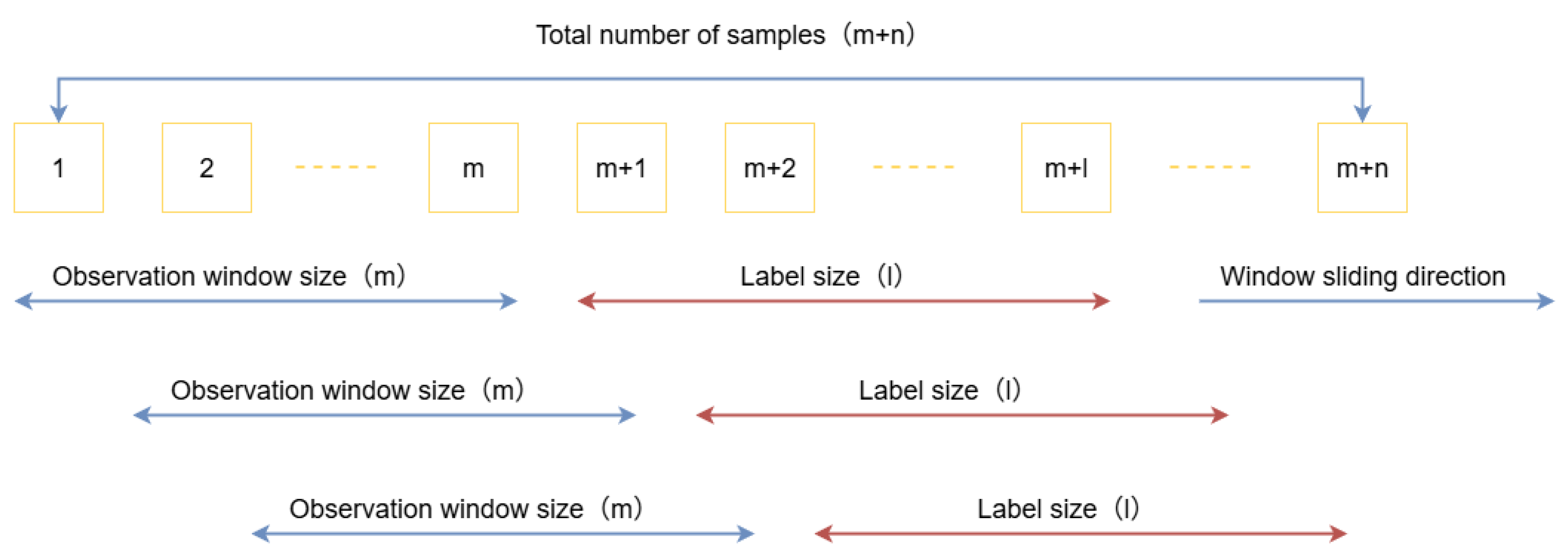
At its core, trajectory prediction is a multi-input, multi-output experiment. It involves predicting the aircraft’s trajectory features for the next few time steps based on a historical time series of inputs. The historical input sequence is called the observation window, and the subsequent time steps are called labels. In the time series, a specific window divider uses a sliding window to move along the data direction, generating the data and labels for training.
Figure 5 illustrates the design of the sliding window, which contains m + n samples in total. The blue line represents the observation window region for sliding training data, and the red line represents the label region for sliding labels, both of which slide along the window’s direction until the data’s end. Each sliding operation yields a training data set, where each trajectory point contains multi-dimensional features: Time, Altitude, Speed, Longitude, Latitude, and Heading. In this experiment, the observation window size and label size are iterated through different values [16], as follows:
Observation window (seq_lengths) = [10, 20, 30, 40, 50]
Labels (forecast_lengths) = [1, 2, 3, 4, 5]
By evaluating the overall performance metrics across all features, we select the optimal observation window size and label size to achieve high-precision four-dimensional trajectory prediction.

4.2. Prediction Model

4.2.1. Construction of a Spatio-Temporal Graph

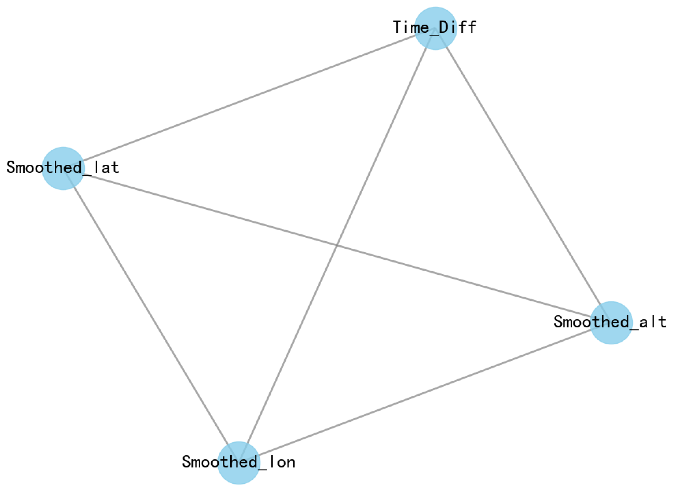
The spatio-temporal graph is represented by the graph-theoretic notation “ G t = V , E t , A t ,” where V denotes the set of nodes, represents the set of edges at time t, and A t denotes the adjacency matrix [17] at time t. The spatio-temporal graph constructed in this experiment is a static undirected graph. The four-dimensional trajectory feature variables from the preprocessed trajectory sequence are used as nodes, namely Time_Diff, Smoothed_lat, Smoothed_alt, and Smoothed_lon, to construct an undirected graph structure. This structure represents the relationships between these features, reflecting the spatio-temporal associations among different features, and lays the foundation for the subsequent construction of the STGNN model. The spatio-temporal graph structure is shown in Figure 6.

4.2.2. Spatial Learning Networks (GAT)

The Graph Attention Network (GAT) uses an attention mechanism to assign different weights to each node in the graph based on the features of its neighboring nodes, capturing more complex relationships between nodes and thereby improving the accuracy of model predictions [18]. GAT captures the relationships between nodes in the graph. It applies a multi-head attention mechanism to each node’s features to extract the trajectory data’s spatial features. The specific steps for implementing the Graph Attention Network are outlined below.
First, calculate the attention coefficients. For vertex i, calculate the similarity coefficients between its neighboring nodes j and itself.
e i j = a W h i , W h j
In Formula (5), W h i denotes the linear transformation of nodes i and j using shared parameters W and h i , followed by concatenating the transformed results and mapping the concatenated features to real numbers a. Then the attention coefficients are normalized so that the attention weights of all neighbor nodes are added to 1, so as to ensure that the information of all neighbor nodes can be reasonably integrated into the target node i. The normalization process is shown in Formula (6):
α i j = s o f t m a x j e i j = exp e i j k N i   exp e i k
In Formula (6),   N i represents a neighbor node of node i in the graph.
The complete attention coefficient calculation is shown in Formula (7):
α i j = exp L e a k y R e L U a T W h i W h j k N i   e x p L e a k y R e L U a T W h i W h k
In Formula (7), || represents the vector concatenation operation, and LeakyReLU is the activation function.
Then, perform weighted aggregation. Based on the normalized attention coefficients α i j , the feature vectors h j of the neighboring nodes of node i are weighted and summed to obtain the new feature vector h i of node i.
h i = σ j N i   α i j W h j
In Formula (8), σ denotes the activation function.
A multi-head graph attention layer enhances the expressive power of the attention mechanism. The model can fully consider the correlations between nodes by learning multiple sets of varying attention mechanisms. The calculation is shown in Formula (9):
h i = | | k = 1 k σ j N i   α i j k W k h j
In Formula (9), || denotes the concatenation operation, k denotes the number of heads, α i j k denotes the attention coefficients calculated by the kth group of attention mechanisms, and W k denotes the corresponding linear transformation matrix.
The GAT extracts spatial features from the trajectory data. It can process three-dimensional input tensors containing trajectory data at different time steps and nodes. Then, a bidirectional attention mechanism is introduced to enable GAT to capture more complex relationships between nodes, outputting the spatial feature matrix of each node, S ( t ) , as shown in Formula (10). These features can then be used to construct the spatial learning network part of the spatio-temporal graph neural network (STGNN) for trajectory prediction.
S t = G A T h i t , X t
In Formula (10), h i t represents the feature vector of node i under the bidirectional attention mechanism, and X t represents the t-th trajectory point.

4.2.3. Temporal Learning Network (BiGRU)

To resolve the gradient vanishing challenge in traditional recurrent neural networks (RNNs), the gated recurrent unit (GRU) model [19] was developed as an enhanced RNN architecture incorporating a gating mechanism. Compared to long short-term memory recurrent neural networks (LSTMs), GRUs have fewer parameters and lower computational complexity and perform better when handling long-term dependencies.
GRUs primarily consist of an update gate and a reset gate. The update gate determines whether the current input should be updated relative to the current state information, thereby selecting more relevant information. The reset gate determines which past state information to retain, combining past states with the current input state. The specific model computation process is shown in Formulas (11)–(14):
z t = σ W z h t 1 , x t
r t = σ W r h t 1 , x t
h ~ t = tanh W r t h t 1 , x t
h t = 1 z t h t 1 + z t h ~ t
In Formulas (11)–(14), t denotes the time of the current state; z t denotes the update gate; r t denotes the reset gate; h ~ t denotes the candidate hidden state; h t denotes the final hidden state; h t 1 represents the hidden state of the previous time step; x t denotes the current state information; W z , W r , and W denote the weight matrices corresponding to different gates; σ denotes the sigmoid activation function; and denotes the dot product.
The bidirectional gated recurrent unit (BiGRU) [20] is introduced based on GRU to account for both forward and backwards information in time series. BiGRU consists of two independent GRUs, one processing sequence data in forward order and the other in reverse order. The model structure is shown in Figure 7:
For the forward GRU, the hidden layer state sequence is h 1 , h 2 , …, h 3 . Following the conventional GRU computation method, the hidden layer states are computed sequentially from the start position to the end position of the sequence data.
For backward GRU, the hidden layer state sequence is h t , h t 1 , …, h 1 , which is calculated in reverse order from the end position of the sequence data to the start position of the sequence data.
After obtaining the forward and backwards hidden layer state sequence data, BiGRU concatenates the forward hidden layer and backward hidden layer at each time step to get the final hidden state information h t .

4.2.4. Temporal Pattern Attention Mechanism (TPA)

By introducing the TPA [21] attention mechanism, the time features extracted by BiGRU are weighted and aggregated to highlight important temporal patterns, further enhancing the model’s prediction capabilities.
The TPA attention mechanism is used to process time series data. It introduces the concept of temporal patterns on top of the traditional attention mechanism to capture essential patterns and features in time series. In this experiment, the feature sequence matrix h t extracted from the final hidden states by BiGRU is passed to k one-dimensional CNN filters C j R 1 × w of length w . Each filter performs convolution on each feature of the m hidden states, generating a matrix H C R m × k with m rows and k columns. The convolution process is shown in Formula (15):
H i , j C = l = 1 w   H i , t w 1 + l × C j , T w + l
Then, the scoring function compares the final hidden states extracted by BiGRU ( h t ) with the scores, as shown in Formula (16). A weight is calculated for each row of H C , normalised, and activated via the Sigmoid function, allowing multiple time series to be considered simultaneously. The activation function is shown in Formula (17), which sums the rows of H C weighted by their corresponding weights to generate v t . The summation formula is shown in Formula (18). Finally, concatenate V t with h t and perform matrix multiplication to generate the final h t , as shown in Formula (19).
f H i C , h t = H i C W a h t
α i = s i g m o i d f ( H i C , h t )
v t = i = 1 n α i H i C
h t = W h h t + W v v t
In Formula (16), H i C is the i-th row of H C , and W a R k × m . In Formula (19), h t , h t R m , W h R m × m , and W v R m × k .

4.2.5. Spatio-Temporal Fusion Network Architecture

The spatio-temporal fusion network architecture integrates spatial and temporal learning networks into a complete STGNN. After preprocessing the trajectory data, spatial feature matrices are extracted using GAT ( S ( t ) ), and temporal features are extracted using BiGRU-TPA ( h t ). These are then stacked layer by layer to form feature vectors that combine spatio-temporal features ( H t ). The spatio-temporal fusion network architecture is shown in Figure 8.

4.2.6. Training and Prediction Module

The training prediction module in the STGNN model utilizes a single-layer GRU, which takes the feature vector H t of the fused spatio-temporal features as input to the GRU network layer to process the time series data. At every prediction step, the GRU processes both the input and the current hidden states, subsequently generating the output for the present time step together with an updated set of hidden states. Then, through a fully connected layer [22], the GRU output is converted into prediction results, which are stored in a list. A feedback mechanism uses the prediction results as input for the next time step, enabling multi-step prediction of future trajectory data.

5. Experimental Simulation

5.1. Experimental Environment and Model Parameter Settings

A GAT-BiGRU-TPA trajectory prediction model based on spatio-temporal graph neural networks was designed using the PyTorch 2.7.0 deep learning framework. Input data comprised historical trajectory data points from nine flights departing Beijing Capital International Airport for Shanghai Hongqiao International Airport, with a 10 s data interval. These trajectory data encompass aircraft phases including take-off, climb, departure, cruise, approach, and landing. This experiment conducts predictive analysis on the full trajectory data points. The experimental methodology flowchart is illustrated in Figure 9. The trajectory points are split into 70% for training, 15% for validation, and 15% for testing. The model’s input data comprises six-dimensional features: time, altitude, speed, heading, longitude, and latitude. The model outputs the altitude, longitude, and latitude features for the next time step.
The spatial learning network component processes spatial information in the data, employing a GAT layer with an output feature dimension of 8 and two attention heads to learn feature representations across different spatial domains. The temporal learning network uses BiGRU to extract temporal information from the data, with an input feature dimension of 64 and an output feature dimension of 32. A TPA module further fuses temporal information, generating attention weights through linear transformation and the tanh activation function. Finally, in the prediction stage, a unidirectional GRU layer is used with input and output feature dimensions of 64, followed by a fully connected layer to map the GRU output to the four predicted feature dimensions (time, longitude, latitude, and altitude). Since different input observation window sizes and future label lengths yield different results during model training, a grid search is conducted for observation window and label sizes, with the observation window size set to [10, 20, 30, 40, 50] and the label size set to [1, 2, 3, 4, 5]. The hardware and software configuration for the experiment is shown in Table 2. The model parameters are set as shown in Table 3.

5.2. Evaluation Metrics for Model Error

The root mean square error (RMSE) and mean absolute error (MAE) are used as evaluation metrics for error [23], where RMSE is the square root of the mean of the squares of the differences between the actual values and the predicted values. It measures the average magnitude of the errors between predicted and actual values, amplifying the differences between larger errors. The calculation is shown in Formula (20). MAE is the average of the absolute differences between the actual and predicted values, reflecting the true error. It assigns equal weights to all mistakes and is unaffected by extreme outliers. The calculation is shown in Formula (21). The smaller the values of RMSE and MAE, the better the model’s fitting performance.
R M S E = 1 n i = 1 n   ( y i y ^ i ) 2
M A E = 1 n i = 1 n   y i y ^ i
In Formulas (20) and (21), n denotes the total sample count, y i indicates the truth value for the i-th sample, and y ^ i signifies its corresponding predicted value.

5.3. Comparison with the Baseline Model

Four commonly used neural network models—BiGRU model, BiLSTM model [24], Attention + LSTM model [25], and Attention + GRU + LSTM model [26]—were selected as benchmark models. These benchmark models were compared with the model proposed in this experiment (GAT-BiGRU-TPA) to highlight the effectiveness of the proposed model. To ensure the fairness of the comparison experiment, the same proportion of training, validation, and test sets was used for both the experimental and benchmark models, and a fixed random seed was employed. The results of the trajectory prediction error evaluation indicators for different observation windows, along with the experimental model’s labels, are shown in Table 4. Table 5 shows the average values of the overall error evaluation indicators of the trajectory features of the experimental model.
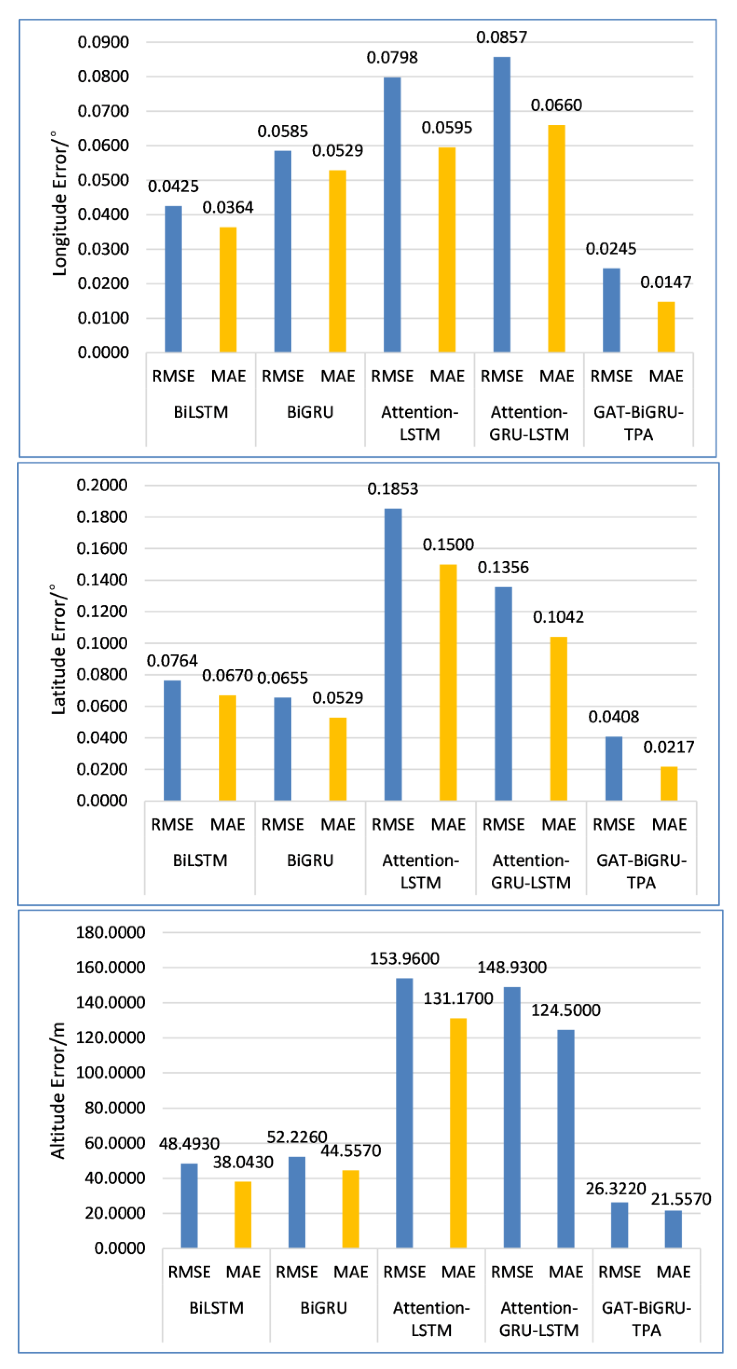
As shown in Table 4 and Table 5 above, the error evaluation metrics RMSE and MAE for the experimental model’s trajectory features (longitude, latitude, and altitude) are presented for different observation windows and labels. The optimal model parameters of the experimental model are obtained as follows: For an observation window of 30 and 4 labels, the overall average error evaluation metrics are RMSE = 2.9245 and MAE = 2.8852. To validate the efficacy of this experimental model, a new trajectory data set was selected for comparative trajectory prediction experiments across different models. For the GAT-BiGRU-TPA model’s optimal parameters—specifically predicting the trajectories of 4 future trajectory points after inputting 30 historical trajectory points—the overall mean prediction error on target features was compared against the baseline model. The specific comparison results are presented in Table 6 below. To present the comparison results more intuitively, a bar chart is plotted as shown in Figure 10.
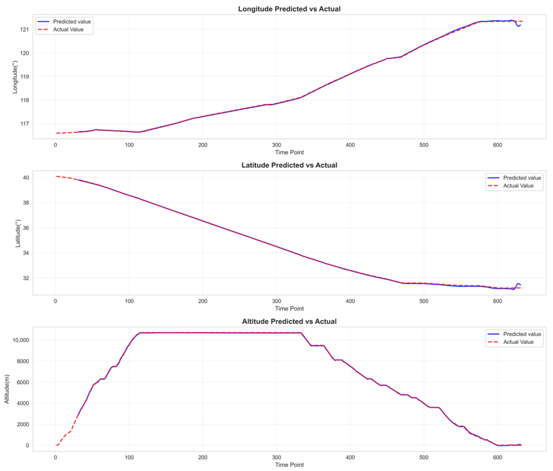
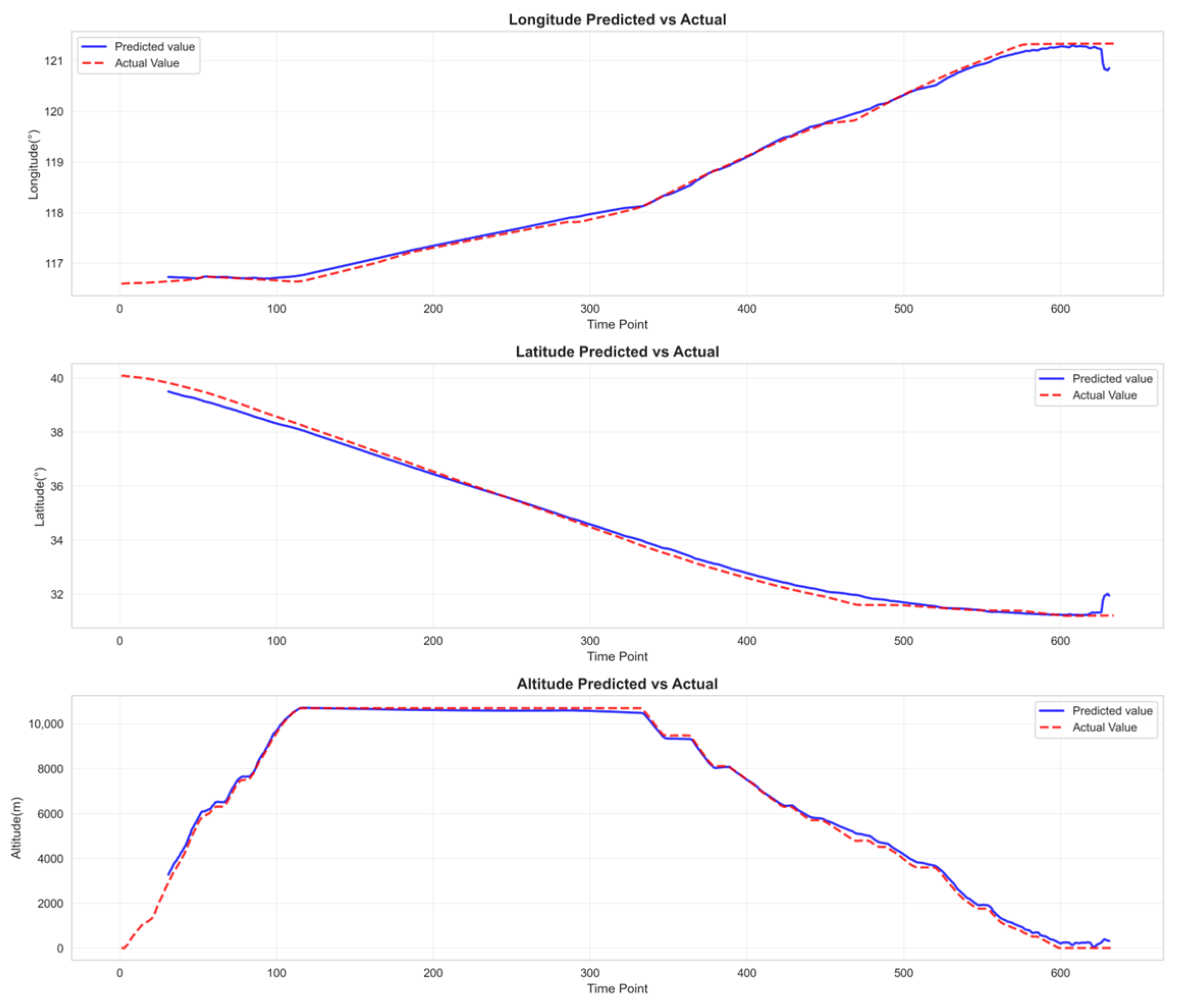
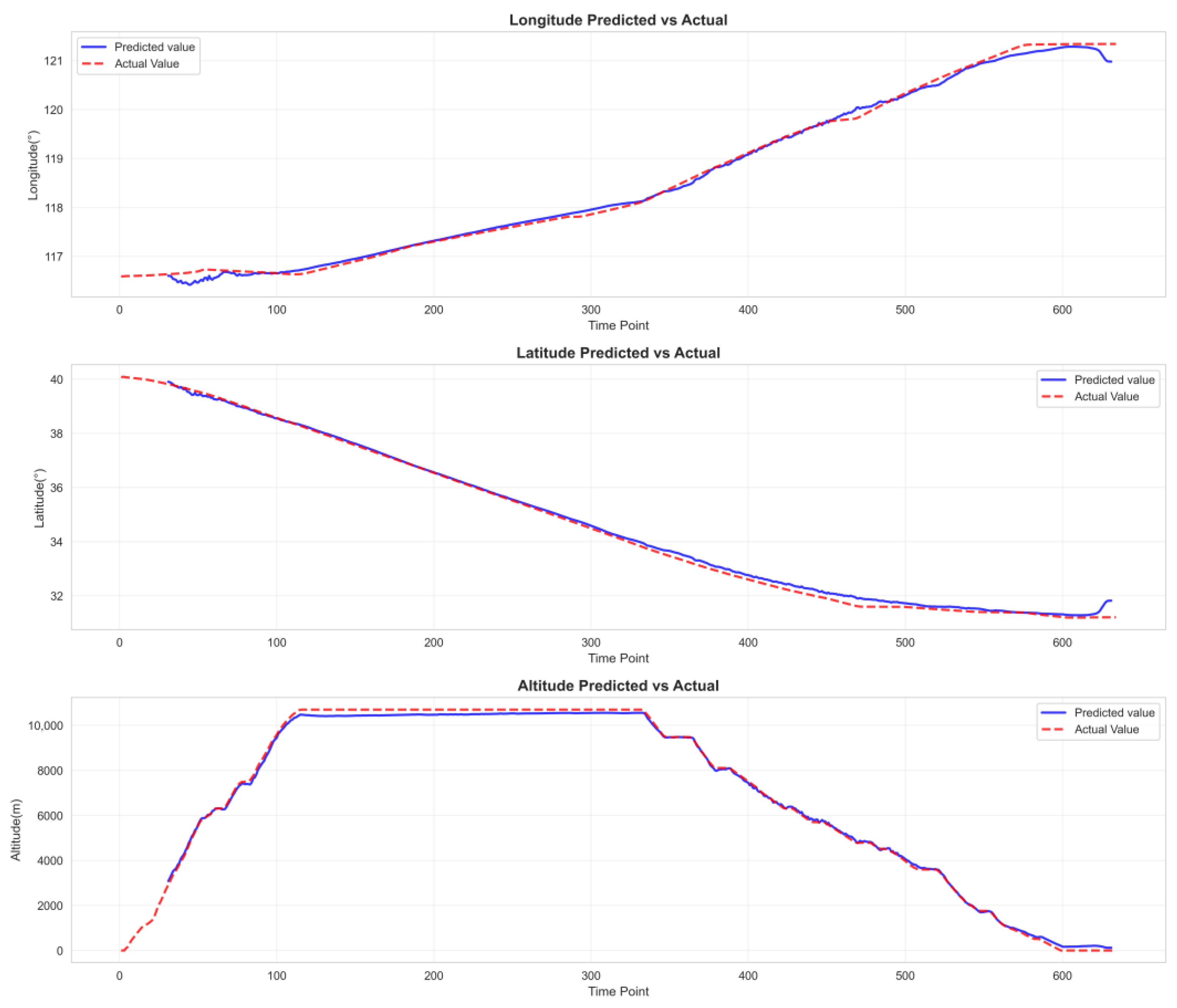
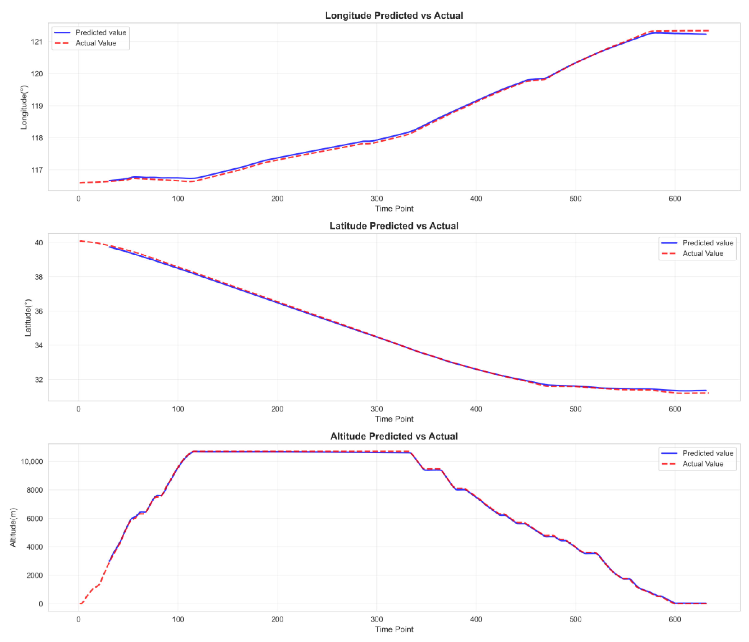
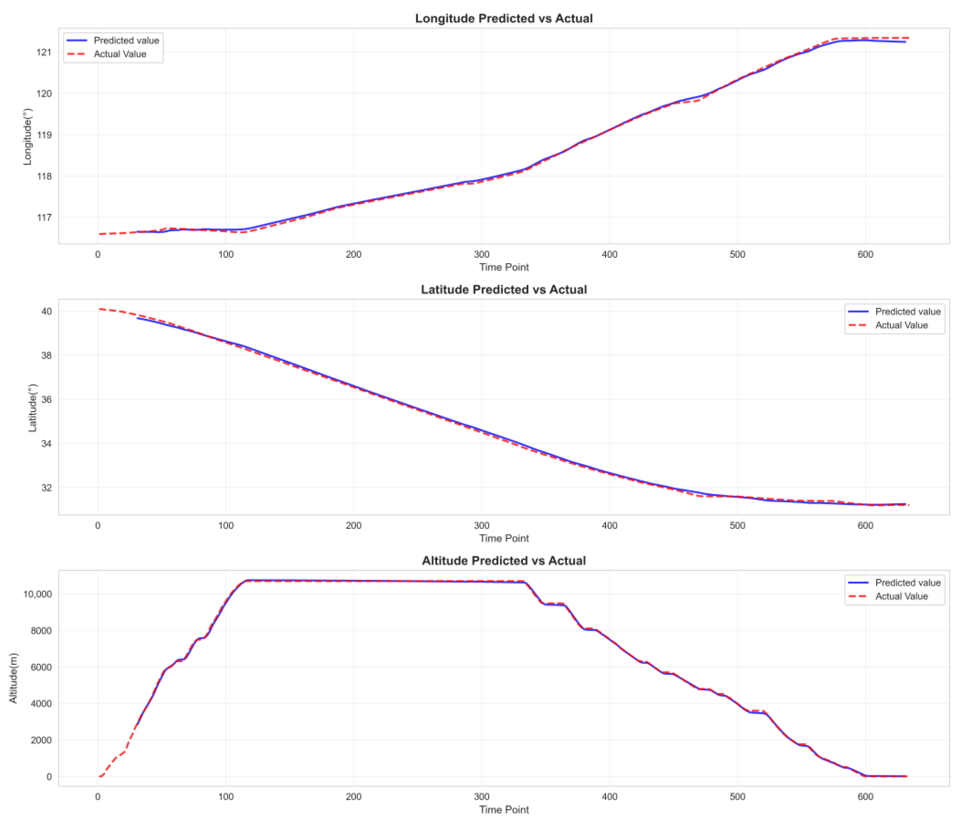
Table 5 clearly demonstrates that the experimental model (GAT-BiGRU-TPA) achieves the lowest prediction error metrics—RMSE and MAE—and the highest prediction accuracy when the observation window is set to 30 and the label count is 4. Compared to the optimal baseline model BiLSTM, the experimental model GAT-BiGRU-TPA reduces RMSE by 45.72% and MAE by 43.40%. Figure 9 demonstrates that our experimental model (GAT-BiGRU-TPA) exhibits lower errors than the baseline model across longitude, latitude, and altitude. Notably, the evaluation metrics for altitude feature predictions are significantly smaller than those of the baseline model, indicating superior predictive performance of our experimental model. Figure 11, Figure 12, Figure 13, Figure 14 and Figure 15 present the fitted curves of predicted versus actual values for target features across different models. The experimental model (GAT-BiGRU-TPA) demonstrates the best fitting performance, further validating its effectiveness.
Based on the results of the RMSE and MAE evaluation metrics, alongside the fitted images of predicted and actual values across the aforementioned experimental models, it is evident that the proposed prediction model exhibits lower prediction errors compared to current mainstream models, yielding more accurate results for target feature prediction. To a certain extent, the prediction outcomes can mitigate collision risks between multiple aircraft, thereby providing a means to ensure the safe and stable operation of air traffic management.

5.4. Quantification of Uncertainty in Predictive Models

In real-world air traffic management (ATM), trajectory prediction must account for multiple uncertainties, including weather, traffic, and aircraft performance. As this experimental model outputs predictions for individual trajectory points, confidence intervals are added to the trajectory predictions to quantify uncertainty, thereby enabling the results to inform ATM decision-making.
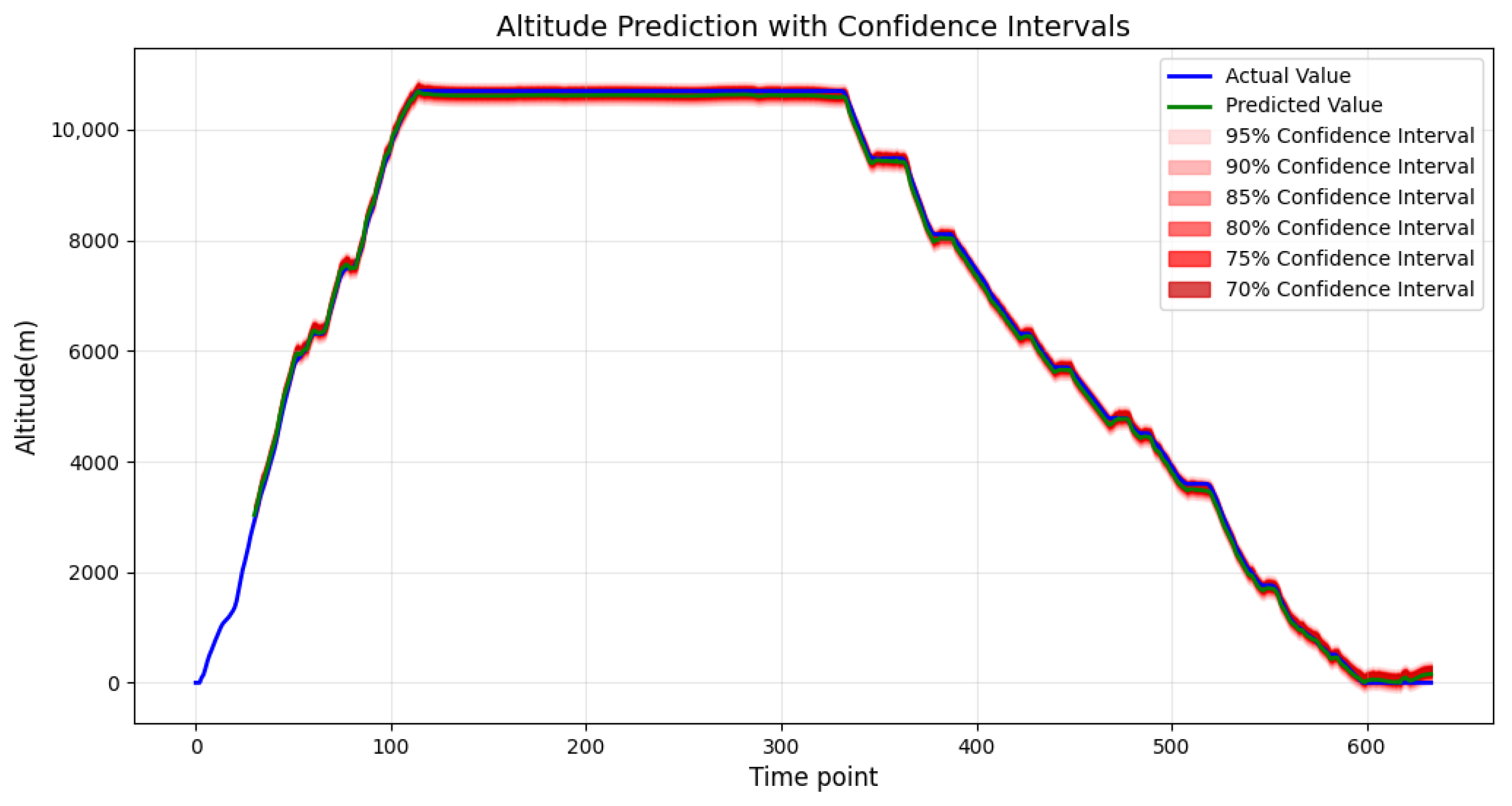
Estimate confidence intervals using residual quantiles. Employ the trained GAT-BiGRU-TPA model to predict the test set, calculating the predicted residuals for the longitude, latitude, and altitude features—that is, the difference between actual and predicted values—as shown in Formula (22). Perform quantile analysis on the residuals for each feature to determine the residual boundaries corresponding to different confidence levels (70%, 75%, 80%, 85%, 90%, 95%). Then, overlay these residual boundaries onto the predicted values of the new trajectory to obtain the confidence interval for each prediction point. The calculation process is shown in Formula (23):
= y a c t u a l y ^ p r e d
C I α = [ y ^ p r e d + q l o w , y ^ p r e d + q h i g h ]
In Formulas (22) and (23), y a c t u a l denotes the actual trajectory value, y ^ p r e d denotes the predicted trajectory value, q l o w denotes the lower quantile of residuals, l o w = 1 α 2 , q h i g h denotes the upper quantile of residuals, l o w = 1 α 2 , α denotes the confidence level.
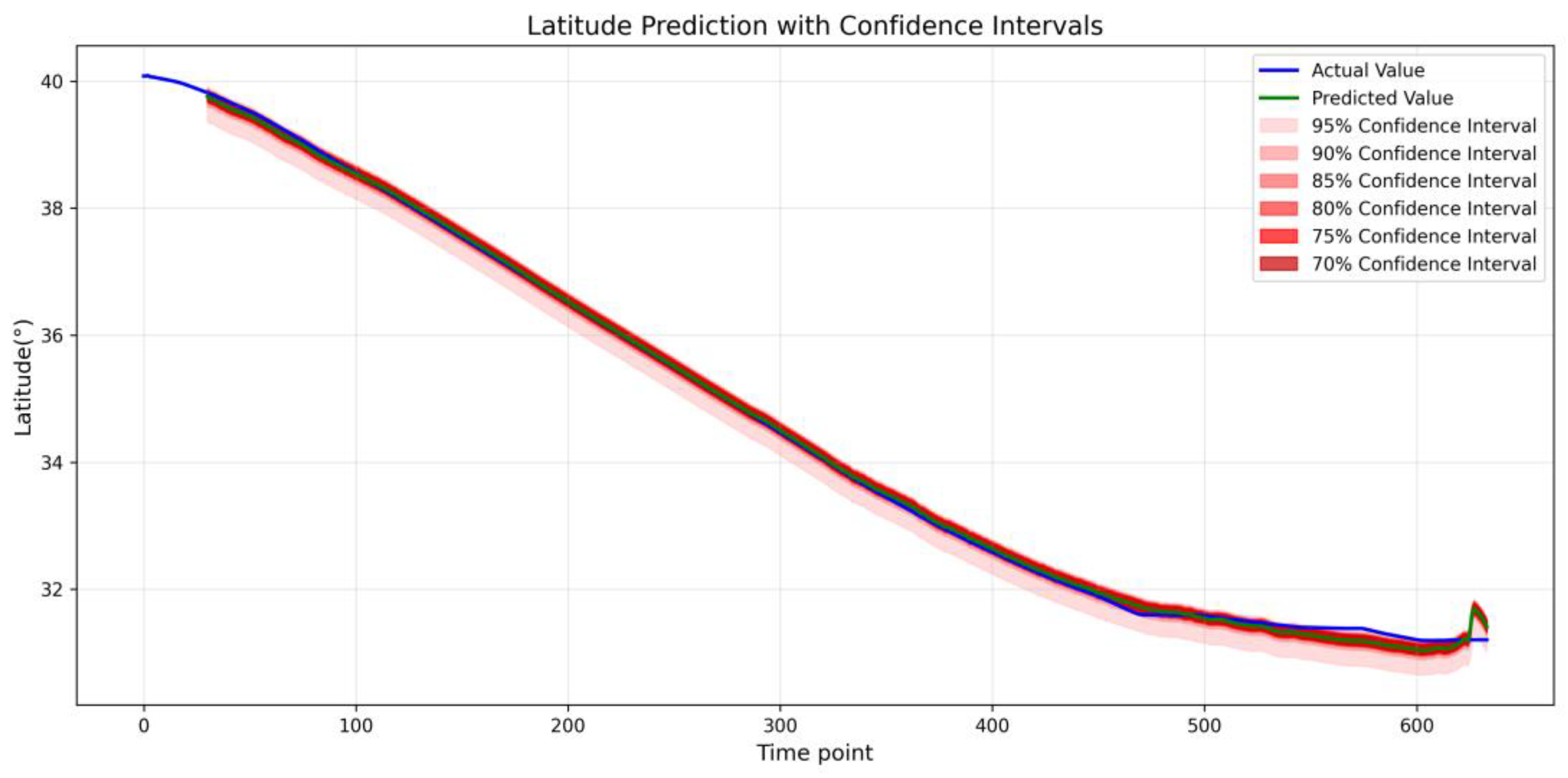
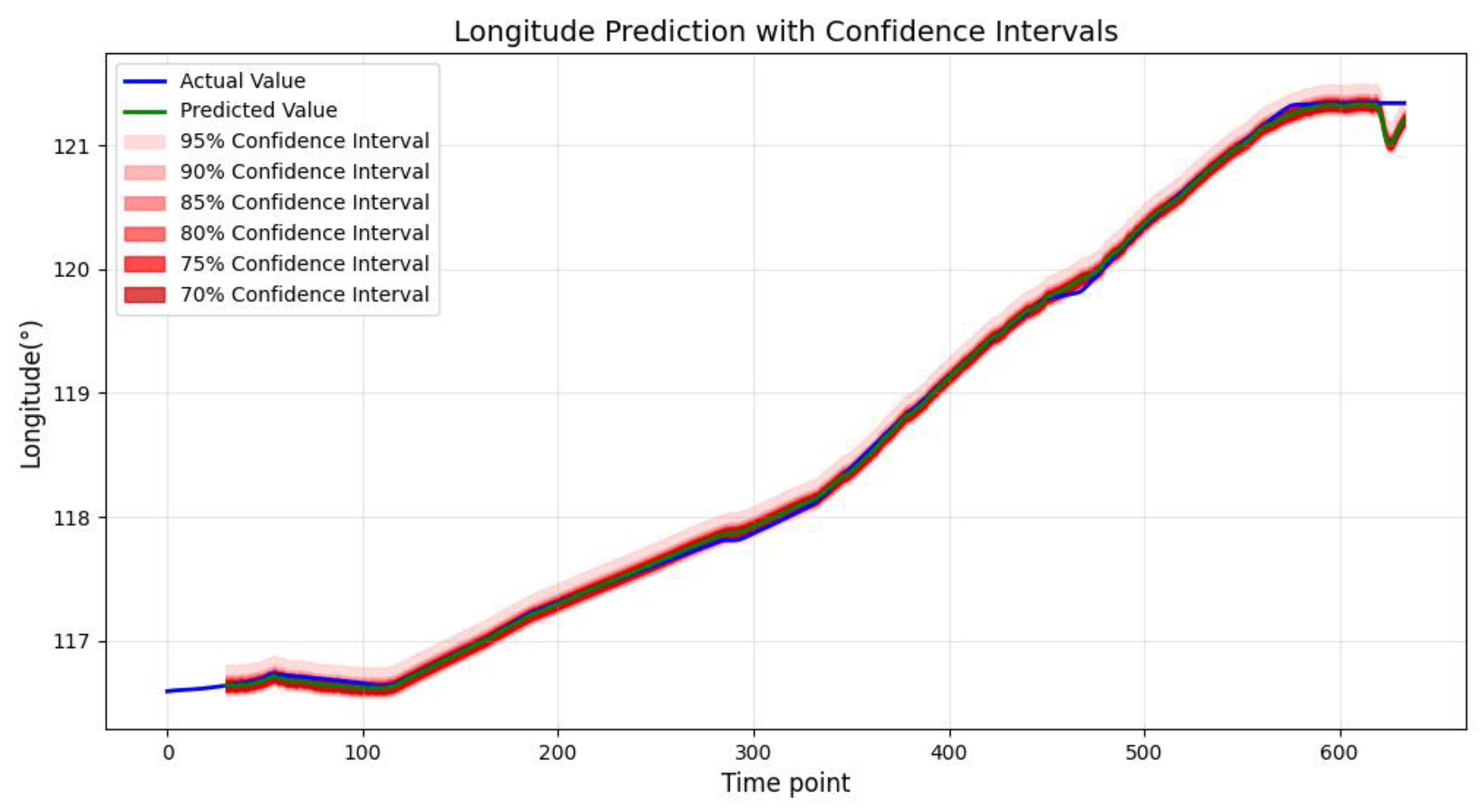
Figure 16, Figure 17 and Figure 18 present an uncertainty analysis of trajectory point predictions using residual quantiles, where the solid blue line denotes actual observations and the solid green line represents model predictions. The predicted results generally align well with the overall trend of actual values. The red regions respectively indicate multiple confidence intervals at 95%, 90%, 85%, 80%, 75%, and 70%, intuitively reflecting the range of model prediction uncertainty. As the trajectory points change, the confidence intervals of the predicted values fluctuate in width but remain broadly stable overall. This indicates that the model effectively captures the trend of actual values across different trajectory points. These results demonstrate that residual quantiles exhibit good fitting performance when handling complex datasets, while simultaneously assessing prediction reliability through uncertainty intervals.

5.5. Analysis of Prediction Results Under Different Flight States

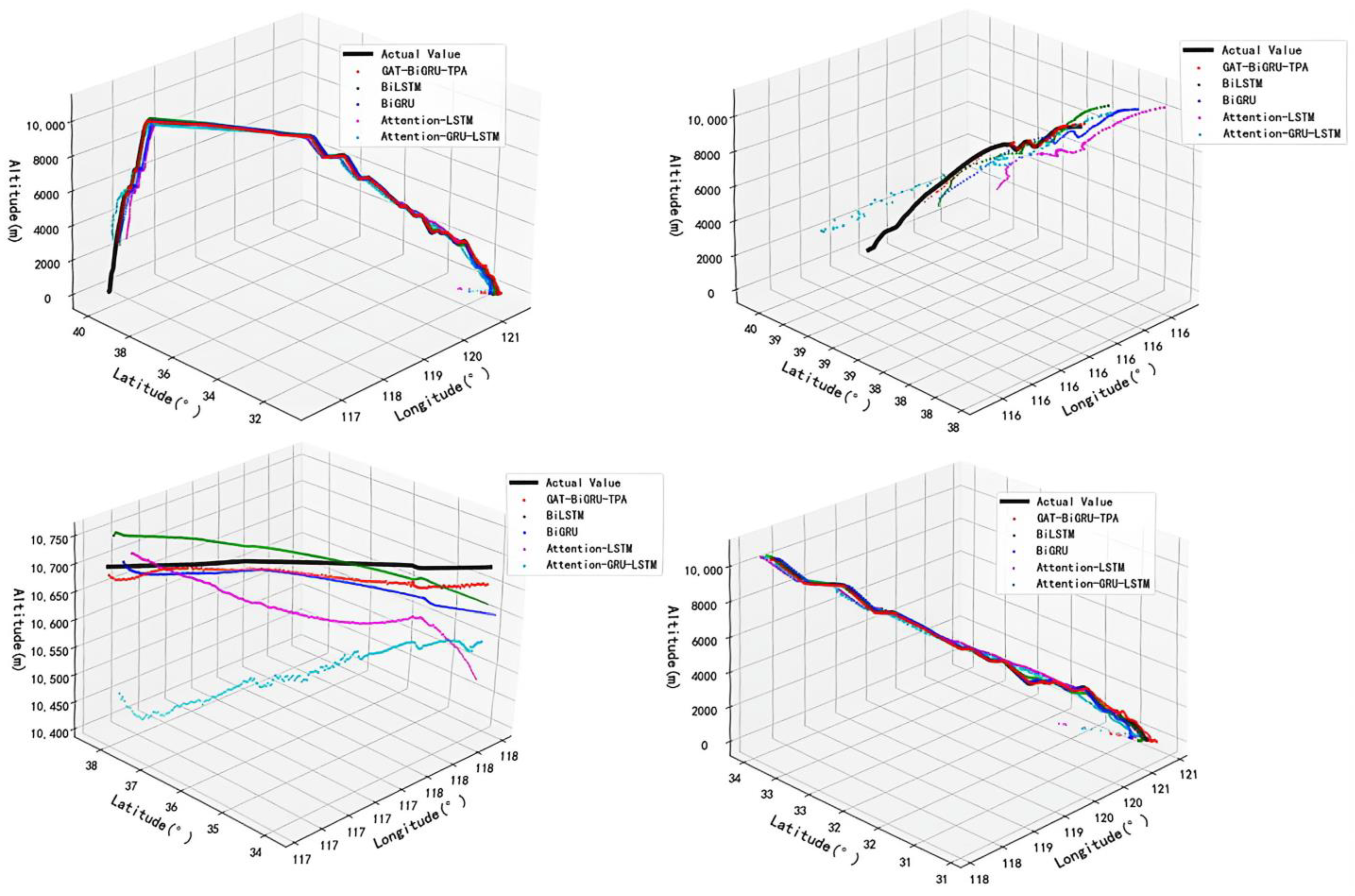
The newly selected trajectory data were loaded into five distinct experimental models: BiGRU, BiLSTM, Attention-LSTM, Attention-GRU-LSTM, and GAT-BiGRU-TPA. With an observation window size of 30 and a label size of 4, the predictive performance of these five models under different flight states was evaluated. As depicted in Figure 19, three-dimensional visualizations of predicted trajectories for different models are shown for the entire trajectory, the departure climb phase, the cruise phase, and the approach descent phase. Detailed error metrics for each phase are presented in Table 7.
In Figure 19, different colours denote trajectory points predicted by distinct models: the black segment represents the actual trajectory; the red segment indicates the trajectory predicted by the model under examination; the green segment shows the trajectory predicted by the BiLSTM model; the blue segment displays the trajectory predicted by the BiGRU model; the purple segment depicts the trajectory predicted by the Attention-LSTM model; and the cyan segment illustrates the trajectory predicted by the Attention-GRU-LSTM model. During the aircraft departure climb phase, the experimental model demonstrates the most favourable fit between its predicted trajectory and the actual trajectory. As shown in Table 7, during this phase, the experimental model achieves a 48.65% reduction in RMSE and a 50.12% decrease in MAE compared to the optimal benchmark model—the BiGRU model. The effectiveness of the experimental model is particularly evident during the aircraft’s cruise phase, where the Attention-GRU-LSTM model exhibits the poorest fitting performance. As shown in Table 7, during the cruise phase, compared to the optimal benchmark model—the BiLSTM model—the experimental model achieves a 30.42% reduction in RMSE and a 25.01% decrease in MAE. During the aircraft’s approach descent phase, the flight attitude undergoes significant changes within a short timeframe. In this complex flight scenario, the baseline model’s predicted trajectory generally aligns with the actual trajectory. However, the experimental model’s predicted trajectory closely matches the actual trajectory, demonstrating superior predictive performance. As shown in Table 7, during the approach descent phase, compared to the optimal baseline model—the BiLSTM model—the experimental model achieved a 45.78% reduction in RMSE and and a 46.68% reduction in MAE.
In summary, the STGNN-based GAT-BiGRU-TPA trajectory prediction model demonstrates robust performance across the entire trajectory, including departure climb, cruise, and approach descent phases. It accurately reflects the aircraft’s state during different flight stages while exhibiting low prediction error.

6. Conclusions

This experiment employs a four-dimensional trajectory prediction model based on the STGNN framework, which integrates GAT, BiGRU, and TPA layers to form a comprehensive spatio-temporal fusion neural network. By comparing this model with certain experimental models mentioned in the introduction, it not only addresses the issues of vanishing gradients and exploding gradients inherent in traditional experimental models but also effectively extracts the spatially interdependent information between each feature within the trajectory data. While simultaneously highlighting critical temporal patterns within the trajectory data to achieve deep spatio-temporal feature integration. Furthermore, uncertainty quantification analysis is applied to the experimental results, extending beyond conventional single-point trajectory prediction. By employing residual quantiles to establish confidence intervals for predictions, the model enhances the reference value and safety of its outputs for practical ATM decision-making. Additionally, the predicted outcomes can serve as a foundation for subsequent multi-aircraft conflict detection, providing reliable basis for conflict assessment among multiple aircraft. The conclusions validated through experimentation are presented as follows:
  • By combining the autoencoder and moving average smoothing method for outlier detection and handling, a high-quality trajectory time series is obtained, reducing the model’s prediction error and improving its prediction accuracy.
  • By using GAT and BiGRU as the spatial feature extraction network and temporal feature extraction network, respectively, the model can fully extract the spatial and temporal features of four-dimensional trajectory data. Additionally, the TPA attention mechanism is integrated to extract important temporal patterns in the trajectory data, increasing the model’s focus on critical feature timings and improving prediction accuracy.
  • After thoroughly considering different observation windows and labels, we compared the RMSE and MAE values of the model predictions corresponding to various observation windows (10, 20, 30, 40, 50) and labels (1, 2, 3, 4, 5). We selected the optimal experimental parameters for the four-dimensional trajectory data in this experiment: observation window = 30 and labels = 4.
  • Under an observation window of 30 and a label of 4, the model proposed in this experiment was compared with traditional trajectory prediction models including BiLSTM, BiGRU, Attention-LSTM, and Attention-GRU-LSTM. Compared to the optimal baseline model BiLSTM, the overall average RMSE for longitude, latitude, and altitude decreased by 45.72%, while the MAE decreased by 43.40%.
  • Transcending conventional single-trajectory point forecasting, the residual quantile method provides confidence intervals for forecast outcomes, intuitively reflecting the scope of model prediction uncertainty. The overall stable trend results effectively evaluate the reliability of the forecasting model.
  • Analysis of the prediction results from different models under various flight conditions indicates that the experimental model exhibits lower prediction errors than the baseline model across all phases of the trajectory, demonstrating favourable predictive performance.
However, the dataset employed for model training and validation in this experiment solely encompasses full trajectory data from various flights operated by a single airline on the Beijing–Shanghai route. Given this singular data source, future research into 4D trajectory prediction will explore collaborations with multiple airlines to gather route data covering diverse aircraft types and broader geographical regions. This will enable the model to learn from a wider range of flight scenarios, thereby further enhancing prediction accuracy. Moreover, numerous unpredictable factors may influence trajectories, such as adverse weather conditions and air traffic congestion. Consequently, future work will incorporate multi-source heterogeneous data to enhance the model’s generalization capability and practical efficiency, thereby advancing the real-world application of predictive models within actual Air Traffic Management systems. In subsequent experiments, we plan to utilise the prediction results from the 4D trajectory prediction model designed in this study to further assess collision risks among multiple aircraft within complex airspace. This will provide more detailed implementation methods for ensuring the safe and stable operation of air traffic management environments.

Author Contributions

Conceptualization, Y.L. and H.C.; methodology, H.C.; software, H.C.; validation, H.C., Y.L., X.M. and Q.G.; formal analysis, Y.L.; investigation, Y.L.; resources, Y.L.; data curation, H.C.; writing—original draft preparation, H.C.; writing—review and editing, H.C., X.M. and Q.G.; visualization, H.C.; supervision, Y.L.; project administration, Y.L.; funding acquisition, Y.L. All authors have read and agreed to the published version of the manuscript.

Funding

This research was funded by the Science and Technology Project of the China Civil Aviation Air Traffic Management Bureau in North China (grant number: 202002) and Tangshan Applied Basic Research Program (grant number: 25130209B).

Data Availability Statement

The trajectory data used in this study are available from https://www.space-track.org/ (accessed on 18 August 2025). The trajectory data used in this study can be obtained from https://flightadsb.variflight.com/(accessed on 4 November 2025).

Acknowledgments

We sincerely thank https://flightadsb.variflight.com/ (accessed on 4 November 2025) for providing the trajectory data, which is the primary data source for the 4D track prediction experiment.

Conflicts of Interest

The authors declare no conflicts of interest.

Abbreviations

The following abbreviations are used in this manuscript:
STGNNSpatio-Temporal Graph Neural Network
GATGraph Attention Network
BiGRUBidirectional Gated Recurrent Unit
TPATemporal Pattern Attention
GRUGated Recurrent Unit
BiLSTMBidirectional Long Short-Term Memory
RMSERoot Mean Square Error
MAEMean Absolute Error
ICAOInternational Civil Aviation Organization
TBOTrajectory-Based Operations
CNNConvolutional Neural Networks
LSTMLong Short-Term Memory
Seq2SeqSequence-To-Sequence
TCNTemporal Convolutional Network
ADS-BAutomatic Dependent Surveillance-Broadcast

References

  1. Ma, L.; Meng, X.; Wu, Z. Data-Driven 4D Trajectory Prediction Model Using Attention-TCN-GRU. Aerospace 2024, 11, 313. [Google Scholar] [CrossRef]
  2. Zeng, W.; Chu, X.; Xu, Z.; Liu, Y.; Quan, Z. Aircraft 4D Trajectory Prediction in Civil Aviation: A Review. Aerospace 2022, 9, 91. [Google Scholar] [CrossRef]
  3. Ma, L.; Tian, S. A Hybrid CNN-LSTM Model for Aircraft 4D Trajectory Prediction. IEEE Access 2020, 8, 134668–134680. [Google Scholar] [CrossRef]
  4. Sahadevan, D.; M, H.P.; Ponnusamy, P.; Gopi, V.P.; Nelli, M.K. Ground-Based 4d Trajectory Prediction Using Bi-Directional LSTM Networks. Appl. Intell. 2022, 52, 16417–16434. [Google Scholar] [CrossRef]
  5. Jia, P.; Chen, H.; Zhang, L.; Han, D. Attention-LSTM Based Prediction Model for Aircraft 4-D Trajectory. Sci. Rep. 2022, 12, 15533. [Google Scholar] [CrossRef]
  6. Luo, A.; Luo, Y.; Liu, H.; Du, W.; Wu, X.; Chen, H.; Yang, H. An Improved Transformer-based Model for Long-term 4D Trajectory Prediction in Civil Aviation. IET Intell. Transp. Syst. 2024, 18, 1588–1598. [Google Scholar]
  7. Shi, Q.Y.; Zhao, W.T.; Han, P. GTA-Seq2Seq multi-step 4D trajectory prediction model based on spatio-temporal feature extraction. J. Beijing Univ. Aeronaut. Astronaut. 2024, 1–16. [Google Scholar] [CrossRef]
  8. Li, H.; Si, Y.; Zhang, Q.; Yan, F. 4D Track Prediction Based on BP Neural Network Optimized by Improved Sparrow Algorithm. Electronics 2025, 14, 1097. [Google Scholar] [CrossRef]
  9. Zhao, Y.D.; Sun, M.Z.; Wang, X.H.; Ke, Y.C. Research on 4D trajectory prediction based on multi-task learning method. J. Beijing Univ. Aeronaut. Astronaut. 2025, 1–14. [Google Scholar] [CrossRef]
  10. Lu, Y.; Chen, S.; Zhang, X.; Pan, X.; Gang, Y.; Wang, C. A Quantum-Enhanced Heuristic Algorithm for Optimizing Aircraft Landing Problems in Low-Altitude Intelligent Transportation Systems. Sci. Rep. 2025, 15, 21606. [Google Scholar] [CrossRef]
  11. Hu, Y.; Yao, Y.; Chen, J.; Wang, Z.; Jia, Q.; Pan, Y. Solving Scalable Multiagent Routing Problems with Reinforcement Learning. IEEE Trans. Neural Netw. Learn. Syst. 2025, 36, 19604–19618. [Google Scholar] [CrossRef]
  12. Liu, G.; Fan, Y.; Zhang, J.; Wen, P.; Lyu, Z.; Yuan, X. Deep Flight Track Clustering Based on Spatial–Temporal Distance and Denoising Auto-Encoding. Expert Syst. Appl. 2022, 198, 116733. [Google Scholar] [CrossRef]
  13. Wang, C.; Jiang, X.F.; Wang, S.M. Research on the quantum effect traffic prediction algorithm oriented towards intuitive reasoning. J. Xidian Univ. 2025, 52, 152–162. [Google Scholar]
  14. Jia, H.; Yang, Y.; An, J.; Fu, R. A Ship Trajectory Prediction Model Based on Attention-BILSTM Optimized by the Whale Optimization Algorithm. Appl. Sci. 2023, 13, 4907. [Google Scholar] [CrossRef]
  15. He, H.Q.; Shi, X.S.; Liu, H.H.; Hui, K.H. Multi-flight Trajectory in Terminal Area Based on Improved Spatio-temporal Model Forecasting Method. J. Beijing Univ. Aeronaut. Astronaut. 2025, 1–16. [Google Scholar] [CrossRef]
  16. Jatesiktat, P.; Lim, G.M.; Kuah, C.W.K.; Ang, W.T. Unsupervised Phase Learning and Extraction from Quasiperiodic Multidimensional Time-Series Data. Appl. Soft Comput. 2020, 93, 106386. [Google Scholar] [CrossRef]
  17. Jin, G.; Liang, Y.; Fang, Y.; Shao, Z.; Huang, J.; Zhang, J.; Zheng, Y. Spatio-Temporal Graph Neural Networks for Predictive Learning in Urban Computing: A Survey. IEEE Trans. Knowl. Data Eng. 2024, 36, 5388–5408. [Google Scholar]
  18. Veličković, P.; Cucurull, G.; Casanova, A.; Romero, A.; Liò, P.; Bengio, Y. Graph Attention Networks. arXiv 2018, arXiv:1710.10903. [Google Scholar] [PubMed]
  19. Zeng, X.; Gao, M.; Zhang, A.; Zhu, J.; Hu, Y.; Chen, P.; Chen, S.; Dong, T.; Zhang, S.; Shi, P. Trajectories Prediction in Multi-Ship Encounters: Utilizing Graph Convolutional Neural Networks with GRU and Self-Attention Mechanism. Comput. Electr. Eng. 2024, 120, 109679. [Google Scholar]
  20. Huang, J.; Ding, W. Aircraft Trajectory Prediction Based on Bayesian Optimized Temporal Convolutional Network–Bidirectional Gated Recurrent Unit Hybrid Neural Network. Int. J. Aerosp. Eng. 2022, 2022, 2086904. [Google Scholar] [CrossRef]
  21. Shih, S.-Y.; Sun, F.-K.; Lee, H. Temporal Pattern Attention for Multivariate Time Series Forecasting. Mach. Learn. 2019, 108, 1421–1441. [Google Scholar] [CrossRef]
  22. Zou, Y.Q.; Zhang, W.S.; Yuan, Y.; Zhao, B.C.; Qiao, Y.F. Traffic Speed Prediction of Road Network based on GCN and GRU Neural Network. Highway 2025, 70, 261–268. [Google Scholar]
  23. Li, S.M.; Song, S.N.; Wang, H.Y.; Wang, D.Y.; Zhao, M. Refined prediction of terminal area traffic congestion based on multimodal spatiotemporal feature fusion. J. Beijing Univ. Aeronaut. Astronaut. 2024, 1–15. [Google Scholar] [CrossRef]
  24. Liu, X.; Wei, W.; Li, Y.; Gao, Y.; Xiao, Z.; Lin, G. Trajectory Prediction and Visual Localization of Snake Robot Based on BiLSTM Neural Network. Appl. Intell. 2023, 53, 27790–27807. [Google Scholar] [CrossRef]
  25. Xue, H.; Huynh, D.Q.; Reynolds, M. A Location-Velocity-Temporal Attention LSTM Model for Pedestrian Trajectory Prediction. IEEE Access 2020, 8, 44576–44589. [Google Scholar] [CrossRef]
  26. Zafar, N.; Haq, I.U.; Chughtai, J.-R.; Shafiq, O. Applying Hybrid LSTM-GRU Model Based on Heterogeneous Data Sources for Traffic Speed Prediction in Urban Areas. Sensors 2022, 22, 3348. [Google Scholar] [CrossRef] [PubMed]
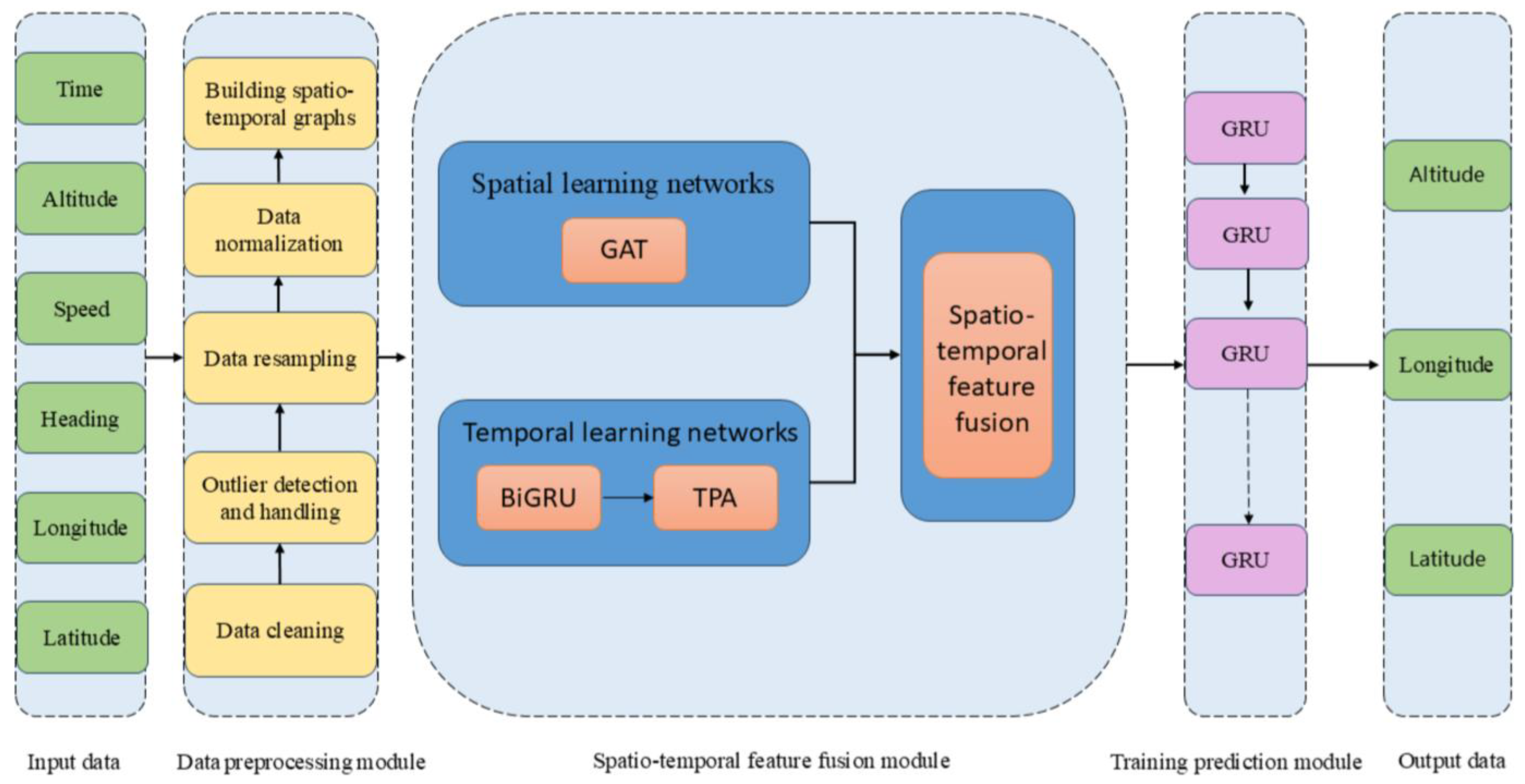
Figure 1. Model framework diagram.
Aerospace 12 00999 g001
Figure 2. Trajectory visualization diagram.
Aerospace 12 00999 g002
Figure 3. Autoencoder network structure diagram.
Aerospace 12 00999 g003
Figure 4. Visualization of preprocessed trajectory.
Aerospace 12 00999 g004
Figure 5. Sliding window.
Aerospace 12 00999 g005
Figure 6. Spatio-temporal graph.
Aerospace 12 00999 g006
Figure 7. BiGRU network structure diagram.
Aerospace 12 00999 g007
Figure 8. Spatio-temporal fusion diagram.
Aerospace 12 00999 g008
Figure 9. Experimental method flowchart.
Aerospace 12 00999 g009
Figure 10. Comparison of prediction errors of target features among different models.
Aerospace 12 00999 g010
Figure 11. GAT-BiGRU-TPA target features prediction fitting curve diagram.
Aerospace 12 00999 g011
Figure 12. Attention-LSTM target feature prediction fitting curve diagram.
Aerospace 12 00999 g012
Figure 13. Attention-GRU-LSTM target feature prediction fitting curve diagram.
Aerospace 12 00999 g013
Figure 14. BiGRU target feature prediction fitting curve diagram.
Aerospace 12 00999 g014
Figure 15. BiLSTM target feature prediction fitting curve diagram.
Aerospace 12 00999 g015
Figure 16. Multi-confidence Intervals for Altitude Prediction Based on Residual Quantile Estimates.
Aerospace 12 00999 g016
Figure 17. Multi-confidence Intervals for Latitude Prediction Based on Residual Quantile Estimates.
Aerospace 12 00999 g017
Figure 18. Multi-confidence Intervals for Longitude Prediction Based on Residual Quantile Estimates.
Aerospace 12 00999 g018
Figure 19. Trajectory fitting curves for different models during distinct flight phases.
Aerospace 12 00999 g019
Table 1. Multiple waypoints for a single flight.
FlightTrajectory PointTimeLongitudeLatitudeAltitudeSpeedHeading
MU5102during the departure phase1 March 2025
08:04:19
116.57140.091646274.096354
MU5102during the cruise phase1 March 2025
08:26:50
116.79538.218711,308892.664166
MU5102during the approach phase1 March 2025
09:42:00
121.33231.2631290233.352176
Table 2. Experimental hardware and software configuration.
Hardware and Software ConfigurationConfiguration NameConfiguration Information
Hardware configurationProcessor13th Gen Intel® Core™ i7-13850HX 2.10 GHz
Graphics cardNVIDIA RTX 3500 Ada Generation Laptop GPU
Memory32 GB
Software configurationProgramming languagePython 3.10
Programming softwarePycharm 2023.1.2
Foundational frameworkPytorch2.7.0 + cuda12.6
Table 3. Model parameters.
ParameterSetting
GAT spatial output dimension8
Number of GAT attention heads2
BiGRU Time Hidden Layer Dimension32
TPA activation functiontanh
GRU prediction head hidden layer dimension64
OptimizerAdam
Learning rate0.001
Observation window (seq_lengths)[10, 20, 30, 40, 50]
Label (forecast_lengths)[1, 2, 3, 4, 5]
Table 4. Error evaluation index of labels corresponding to different observation windows in the GAT-BiGRU-TPA model.
GAT-BiGRU-TPA
RMSEMAE
1234512345
Longitude error/°100.04080.07190.10280.09280.06340.02230.05490.08320.07290.0360
200.04750.04240.07290.06650.26430.03100.01590.05210.04460.2274
300.05210.07340.06430.05200.26280.04060.05820.04150.02130.2252
400.04080.04230.26270.05150.05850.02050.01440.21020.01860.0249
500.04600.06060.04830.05750.29260.02760.04860.02120.03410.2659
Latitude error/°100.03990.08920.07820.09530.11460.01890.06930.05300.07210.0782
200.06770.04380.10590.08850.30260.05880.01180.08030.05970.2614
300.06970.09990.08680.05950.30230.06250.08970.06100.02320.2596
400.06540.04360.32880.05750.06330.05660.01100.28920.01920.0223
500.05460.06000.05790.08120.34340.03870.04540.03000.06530.2834
Altitude error/m1045.09816.64248.12431.24290.72245.09016.59848.09631.20790.720
2053.26254.29027.48329.82912.46053.26054.26827.40329.82712.456
3055.42070.03048.1718.662067.15055.41269.89748.1698.611367.149
4045.0768.812139.32817.42946.42445.0648.794539.32616.92646.414
5020.59368.23149.57224.61152.51320.50968.20249.52424.59752.510
Table 5. Average overall error of the four-dimensional trajectory for the GAT-BiGRU-TPA model.
GAT-BiGRU-TPA
RMSEMAE
1234512345
Overall error average1015.0605.601016.10210.47730.30015.0445.574116.07710.45130.278
2017.79218.1259.22069.99464.342317.78318.0999.17849.97714.3149
3018.51423.40116.1072.924522.57218.50523.34816.0902.885222.545
4015.0612.966113.3065.846115.51515.0472.940013.2755.654515.487
506.897922.78416.5598.249917.7166.858622.76516.5258.232017.687
Table 6. Error evaluation metrics corresponding to optimal model parameters of different models.
BiGRUBiLSTMAttenton-LSTMAttention-GRU-LSTMGAT-BiGRU-TPA
Best model parametersObservation window = 30
Labels = 4
Observation window = 30
Labels = 4
Observation window = 30
Labels = 4
Observation window = 30
Labels = 4
Observation window = 30
Labels = 4
RMSE17.45016.20451.40749.7178.7959
MAE14.88812.71743.79341.5587.1979
Table 7. Error evaluation metrics for different models across distinct flight phases.
BiGRUBiLSTMAttention-LSTMAttention-GRU-LSTMGAT-BiGRU-TPA
RMSEMAERMSEMAERMSEMAERMSEMAERMSEMAE
Departure climb 21.59518.21024.90821.41063.08153.75943.49737.93111.0899.0826
Cruising15.68513.57311.2579.689633.81829.75869.56067.8027.83297.2664
Approach descent 17.32014.87716.03912.39457.73650.99430.56423.7598.69696.6086
Disclaimer/Publisher’s Note: The statements, opinions and data contained in all publications are solely those of the individual author(s) and contributor(s) and not of MDPI and/or the editor(s). MDPI and/or the editor(s) disclaim responsibility for any injury to people or property resulting from any ideas, methods, instructions or products referred to in the content.