Article

Dynamic Adaptive UAV Path Planning Based on Three-Dimensional Environments

1
College of Civil Aviation, Nanjing University of Aeronautics and Astronautics, Jiangjun Road No. 29, Nanjing 211106, China
2
State Key Laboratory of Air Traffic Management System, Nanjing 210007, China
*
Author to whom correspondence should be addressed.
Aerospace 2025, 12(11), 1000; https://doi.org/10.3390/aerospace12111000 (registering DOI)
Submission received: 28 September 2025 / Revised: 6 November 2025 / Accepted: 6 November 2025 / Published: 8 November 2025
(This article belongs to the Section Aeronautics)

Abstract

Sampling-based algorithms are pivotal for high-dimensional UAV path planning, especially in 3D urban environments. The Rapidly-Exploring Random Tree (RRT) suffers from inadequate sampling methods and a single, fixed sampling policy, which lead to elongated paths and higher computational cost. To address this, we propose a Dynamic Adaptive DACS-RRT* algorithm that builds a dynamic, bidirectional sampling space and fuses low-discrepancy Halton sampling with bridge (narrow-passage) sampling, fundamentally tailoring the sampling process to urban settings. We further construct an adaptive, coordinated sampling strategy that dynamically adjusts between straight-to-goal and frustum-cone expansions by computing their probabilities, thereby overcoming the limitations of a single strategy and strengthening directional guidance. After generating a path, we perform multi-objective smoothing to make UAV trajectories better suited to urban environments. Through simulations in three distinct urban scenarios—and in comparison with five baseline algorithms—DACS-RRT* shows improvements in path length, convergence time, node count, iteration count, obstacle clearance, and turning angle, further validating its practicality in urban settings.

1. Introduction

As the low-altitude economy accelerates and on-demand delivery continues to surge, unmanned aerial vehicles (UAVs) show substantial promise for last-mile logistics in urban environments. Compared with ground transportation, low-altitude air corridors are immune to congestion and enable direct routing, offering time-sensitive supplemental capacity during peak hours, post-disaster emergencies, and in island or mountainous regions [1].
UAV path planning algorithms are generally divided into four categories: Graph search-based methods [2], which compute the shortest path from a start to a goal. However, urban environments are often unstructured, and increasing dimensionality raises computational complexity. Sampling-based graph methods, which generate discrete nodes via random sampling and build a graph for path search, are well suited to high-dimensional, complex settings. Representative examples include RRT [3] and PRM [4], intelligent optimization methods, inspired by natural phenomena or biological behaviors, which typically use swarm cooperation or iterative optimization to seek optimal solutions. Major approaches include genetic algorithms [5], ant colony optimization [6], particle swarm optimization [7], and the grey wolf optimizer [8], machine learning-based methods, which enable data-driven, adaptive decision-making—particularly effective for unknown obstacles, unstructured scenarios, and multi-objective optimization.
To address the low search efficiency and overly long paths of sampling-based RRT algorithms, this paper proposes a 3D UAV path-planning method—Dynamic Adaptive RRT* for urban delivery. Building on an urban environment model, we dynamically adjust the sampling region to reduce the generation of low-value samples. Within the adjusted region, Halton sampling is fused with bridge sampling to produce more uniformly distributed, higher-quality samples. Under a goal-bias strategy, we compute extension probabilities and, with certain probabilities, employ goal-biased straight-to-goal extension (GB) and frustum-cone (truncated cone) sampling; random expansion serves as the baseline, forming a complete expansion scheme. After tree expansion, a PSO-based multi-objective optimization refines the path, followed by interpolation-based smoothing, enabling UAV path planning in urban settings.
This paper makes the following contributions:
(1)
We propose dynamically adjusting the sampling space before expansion. Compared with using the global space, this dynamic adjustment narrows the sampling domain and reduces invalid samples and futile expansions. Guided by search progress and the urban modeling context, we shrink or re-define the sampling region so that samples concentrate in areas more likely to yield feasible paths, thereby reducing low-value points.
(2)
We replace purely random sequences with a Halton–Bridge hybrid sequence that is more uniform, comprehensive, and better aligned with urban models, thereby generating more reasonable samples in 3D space. This fundamentally addresses the inherent under-sampling and over-sampling issues of traditional RRT. As the cornerstone of sampling-based planning, producing well-distributed samples is key to RRT efficiency. Although prior work tackles this indirectly via surrogate strategies, our approach fuses low-discrepancy Halton sequences with Bridge sampling to place samples within gaps between obstacles—enabling entry into narrow corridors—and thus fundamentally resolves the “narrow passage” challenge in urban environments, demonstrating superiority over pseudo-random sampling.
(3)
We introduce a complete, dynamically switchable multi-expansion scheme. Building on RRT*, we coordinate three strategies—goal-biased straight-to-goal extension, frustum-cone (cross-sectional cone) extension, and random extension—and switch among them based on probabilities and conditions. This balanced policy markedly improves rapid convergence, obstacle-avoidance capability, and global solvability for UAV planning in urban environments.
(4)
We propose a path-smoothing strategy that performs multi-objective optimization on the generated path, considering path length, collision cost, safety distance, and smoothness. Using PSO-based path optimization, we globally adjust the route to reduce its length. On this basis, we then apply interpolation-based smoothing to connect piecewise linear waypoints into a smooth curve, making the trajectory more suitable for UAV flight in urban models. The combination ensures both global optimality of the path and practical operability for UAVs in urban environments.
The paper is structured as follows. Section 3 describes the modeling of urban obstacle environments and presents the framework of the Dynamic Adaptive RRT* algorithm. Section 4 provides a comparative analysis of planning performance between the proposed method and four baseline algorithms, validating the effectiveness of Dynamic Adaptive RRT* in urban settings. Finally, we offer recommendations for future research and discuss potential directions for subsequent work.

2. Related Work

Swarm intelligence optimization algorithms, noted for strong global search and parallelism, are widely applied to UAV trajectory planning [9]. Chai et al. [10] proposed a hybrid algorithm that combines a simplified Grey Wolf Optimizer with an improved symbiotic organisms search (HSGWO-MSOS) for UAV path planning, balancing global exploration and local exploitation; simulations show it outperforms traditional methods. Jiang et al. [11] presented a 3D UAV path-planning approach that integrates an improved Grey Wolf Optimizer (GWOLC) with a POMDP-based collision-avoidance strategy: feasible trajectories are generated by GWOLC, while MCTS and an information particle filter tree (IPFT) handle collision avoidance. Gu [12] introduced an improved RIME algorithm (IRIME), which enhances initial population diversity via an ice-crystal diffusion mechanism, boosts global exploration with a high-altitude condensation strategy, and prevents premature convergence through a lattice-weaving strategy, formulating path planning as a multi-constraint optimization problem. Yang et al. [13] (2025b) proposed an improved DBO algorithm based on a landmark operator (LODBO), employing a tent map to diversify initial solutions, a landmark factor to broaden the search range, and an adaptive factor to strengthen global search capability.
Graph search algorithms are widely used in UAV path planning due to their simplicity and ability to handle various constraints. Han et al. [14] proposed an indoor UAV path-planning method based on spatial grid partitioning that reduces modeling complexity while improving planning efficiency and path feasibility, effectively resolving “dead zones” in complex indoor settings and outperforming existing methods in experiments. Yuan et al. [15] introduced an improved Lazy Theta* algorithm. For stealth UAV penetration under integrated air-defense systems, Zhang et al. [16] proposed an enhanced A* algorithm that combines bidirectional sector expansion with variable step-size search, together with a minimum radar cross-section (RCS) strategy to achieve static threat avoidance and dynamic replanning; simulations show superior performance in computational efficiency, path cost, and safety, significantly boosting SUAV survivability. Addressing path planning for a dual–quadrotor cooperative transport system, Rao et al. [17] presented an APF-A* algorithm that integrates artificial potential fields with A*, enabling a leader–follower transport strategy and an optimized heuristic to maintain safe spacing; both simulations and flight tests demonstrate substantial gains in search efficiency and path safety. For UAV path planning, Chen et al. [18] built UAV and region models and formulated the search space as a MILP problem, then improved the A* evaluation function and node-selection strategy to generate optimal trajectories.
As a key direction in UAV path planning, sampling-based algorithms demonstrate strong adaptability and efficiency in complex environments. Lin [19] designed and implemented a closed-loop RRT and three of its improvements, enabling real-time generation of collision-free trajectories for UAVs that avoid dynamic obstacles such as commercial aircraft across diverse scenarios, with effectiveness verified through simulations and flight tests. Obermeyer [20] modeled a fixed-wing UAV reconnaissance task against static ground targets as a polygon-visit Dubins traveling salesman problem, and proposed two sampling-based roadmap algorithms that solve efficiently while guaranteeing asymptotic optimality, making them suitable for online planning and highly scalable. Persson [21] extended the classic A* algorithm to the domain of sampling-based motion planning, proposing an improved method with probabilistic completeness and convergence; through multiple optimization strategies, the approach efficiently produces reliable, high-quality solutions for high-dimensional planning problems.

3. Dynamic Adaptive RRT* Algorithm

Section 3 focuses on urban obstacle modeling and the Dynamic Adaptive RRT* algorithm. Urban obstacle modeling is detailed in Section 3.1. Section 3.2 outlines the overall framework of Dynamic Adaptive RRT*, followed by: Section 3.3 on dynamically adjusting the sampling space; Section 3.4 on fusing Halton and Bridge sequences; Section 3.5 on the goal-biased expansion strategy system; and Section 3.6 on PSO-based optimization and interpolation smoothing.

3.1. Environmental Modeling

When performing transport missions in urban airspace, UAVs encounter a wide variety of obstacles. To reduce onboard computation and improve path-planning efficiency, we first model complex buildings. The experimental scenario is set within a bounded 3D space W = [ 0.2000 ] × [ 0.2000 ] × [ 0.1000 ] , which contains multiple geometric obstacles to simulate UAV path planning in complex environments. Obstacles are defined parametrically as analytic geometric primitives, comprising the following two categories:
Cube: Defined by the center coordinates ( c x , c y , c z ) and edge lengths ( d x , d y , d z ) , denoted as [ c x , c y , c z ; d x , d y , d z ] . Its occupied spatial region is given by Equation (1):
c x d x / 2 , c x + d x / 2 × c y d y / 2 , c y + d y / 2 × c z d z / 2 , c z + d z / 2
Cylinder: Symmetric about the z -axis, defined by center c x , c y , c z , radius r , and height h , denoted as { c x , c y , c z , r , h } . Its occupied spatial region is Equation (2):
{ ( x , y , z ) ( x c x ) 2 + ( y c y ) 2 } r 2 , | z c z | h / 2
In the experimental environment, multiple obstacles are deployed, most of which are rectangular boxes. These obstacles are arranged across different layers and orientations in space, forming a complex 3D blocking structure: obstacles appear at the bottom, along the sides, and in the mid-levels; local areas are connected by narrow corridors; and some regions feature mixed distributions that include cylinders. As a result, the path-planning process must contend with typical challenge scenarios such as narrow passages and dead ends. For ease of visualization and collision checking, all obstacles are rendered via parametric functions, and intersections between points/paths and obstacles are determined using analytic geometric conditions. This modeling approach ensures scene reproducibility while keeping computational costs low, making it suitable for repeated comparative experiments. We simulate rectangular prisms and cylinders as urban building obstacles. The 3D urban environment model is shown in Figure 1.

3.2. Dynamic Adaptive RRT* Algorithm Framework

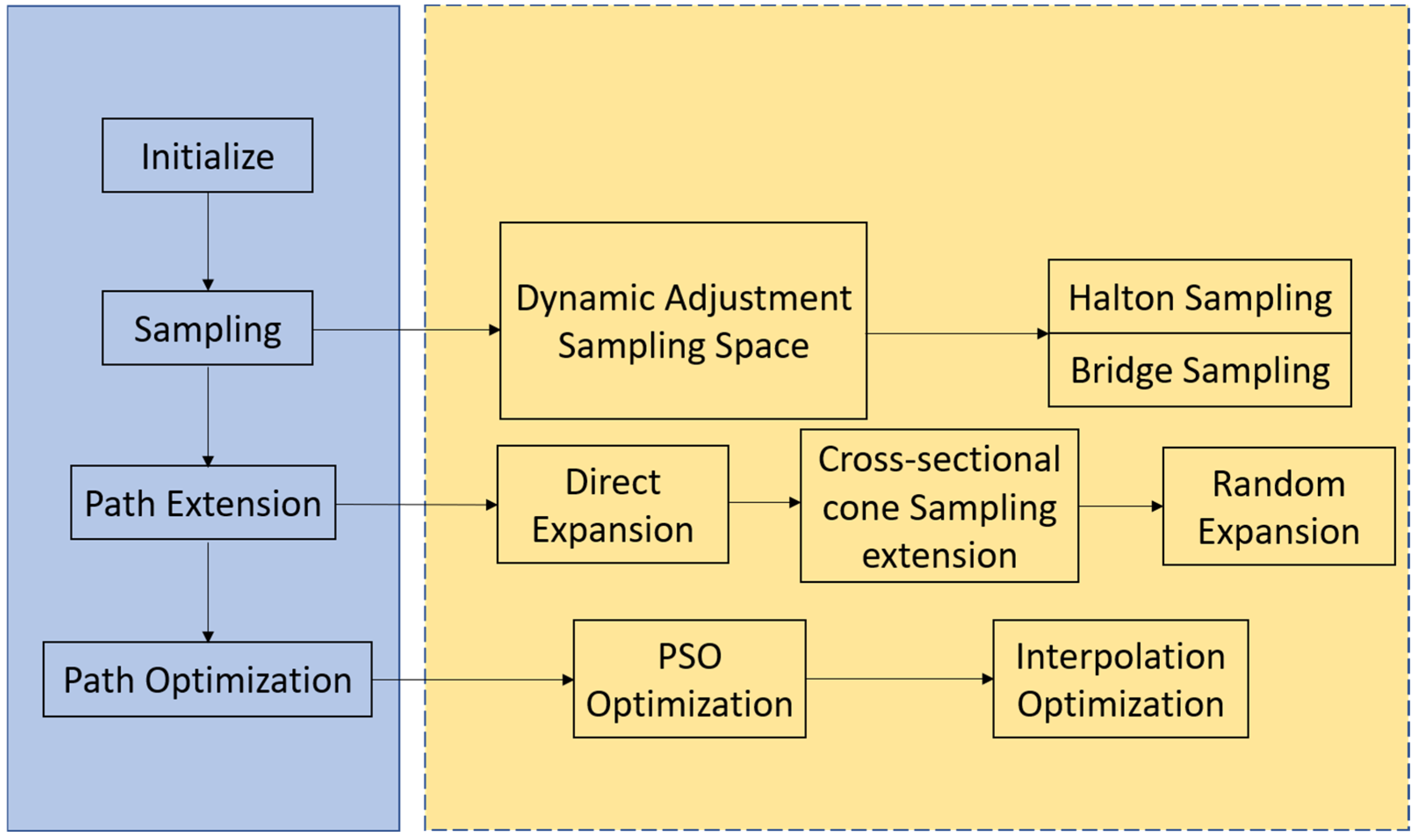
This section presents the flowchart of the Dynamic Adaptive RRT* algorithm. The flowchart is shown in Figure 2.
The blue modules denote the basic pipeline: “Initialization,” “Sampling,” “Path Expansion,” and “Path Optimization.” The yellow modules are the enhanced components. The core idea is to dynamically adjust the sampling space, establish samples via a fusion of Halton and Bridge sampling, construct a layered expansion scheme, and improve the path-optimization stage. The expansion scheme progresses in stages—from goal-biased (GB) straight-to-goal expansion, to frustum-cone (cross-sectional cone) sampling expansion, and finally to random expansion. For path optimization, we first apply multi-objective PSO and then perform interpolation-based smoothing.

3.3. Dynamic Adjustment of Sampling Space

Uniform sampling over the entire space wastes many samples in regions unrelated to the current direction of progress. A fixed-size sampling domain, on the other hand, struggles to balance “rapid long-range exploration” with “fine-grained refinement near the goal,” and tends to stall in narrow gaps or cluttered areas, causing repeated trial-and-error. To address this, we design a dynamically adjusted sampling space during planning: random samples are confined to an axis-aligned window that slides along the start–goal direction, and the window’s scale adapts to search progress and failure feedback. This mechanism significantly reduces invalid sampling and accelerates tree growth in open areas; it actively shrinks near the connection/goal phase to facilitate rewiring and reconnection; and it temporarily enlarges after consecutive expansion failures to bridge narrow passages—thereby improving convergence speed, node utilization, and overall success rate.
Let the start and goal be s , g R 3 , and define the baseline distance d 0 as the absolute distance between them. At the t -th expansion, let the frontier nodes of the two trees—TA grown from the start and TB grown backward from the goal—be q t A and q t B , respectively. We define a normalized progress measure that varies with t: the closer we are to the goal endpoint, the smaller this progress measure becomes. The formulas for q t A and q t B are given in Equation (3).
r t A = q t A g 2 d 0 , r t B = q t B s 2 d 0 , r t A / B 0,1 .
To enable the sampling window to shrink adaptively with progress and to relax automatically when the search stalls, we introduce a dynamic shrinkage index α t and a rollback factor γ t .
Let η t [ 0,1 ] denote the stage-wise completion level, and use an exponential mapping to smoothly interpolate over [ α m i n , α m a x ] . The formulas for dynamic shrinkage index α t are given in Equation (4):
α t = c l i p ( α m i n + ( 1 η t ) h e x p ( α m a x α m i n ) , α m i n , α m a x )
where h e x p > 0 controls the nonlinearity: when η t is large, α t increases slightly, driving the window to shrink more quickly.
The side length of the sampling window is scaled based on the reference distance between the start and end points. First, it is scaled according to the “progress-related radius term (with adaptive exponent) × scheduling coefficient,” and then clipped to the allowed minimum and maximum size range to avoid being too small, which could lead to degeneration, or too large, which could result in ineffective search.
As the search gradually approaches the target (or the starting point), this radius term decreases rapidly, causing the window to shrink monotonically and focus on the connecting region. When consecutive search failures occur, a temporary enlargement strategy is employed to escape local traps; when progress stagnates, the shrinkage rate is increased to enhance focus. Additionally, after a successful expansion, the window is slightly relaxed to maintain necessary exploratory behavior. The above adaptive updates dynamically balance between “shrinking and relaxing,” suppressing oscillations while ensuring both convergence speed and global exploration.
Intuitively, treat the feasible corridor around the straight start–goal line as a reference three-dimensional volume. As the two trees get closer, the linear size of the sampling window scales with the current separation between the trees relative to the start–goal distance. Because volume is the product of three linear dimensions, the window’s volume therefore shrinks roughly with the cube of that ratio. In practical terms, if the inter-tree distance is halved, the window volume drops to about one-eighth. The radius term with exponent α t follows the same cubic-contraction behavior. The process of axis-aligned sliding window is as follows:
Along the three coordinate axes, a cuboid corridor is formed by taking the smaller value of the start and end points on each axis as the lower bound and the larger value as the upper bound, aligned with the line connecting the start and end points and aligned with the axes. Two types of advancing windows are generated within this corridor, both of which are aligned with the coordinate axes and always constrained within the aforementioned corridor. During operation, the two windows advance toward each other synchronously, alternating for sampling and expansion.
(1)
Start-side advancing window: Using the current frontier node of the start tree as a reference, the window center moves forward along the start-to-goal direction; its size scales proportionally with the ‘remaining distance from the start tree to the goal’—the smaller the distance, the tighter the window, guiding forward expansion from the start side.
(2)
Goal-side advancing window: Defined symmetrically with the above, using the current frontier of the goal tree as a reference. The window center advances backward along the start-to-goal direction; its size scales proportionally with the ‘remaining distance from the goal tree to the start point’ and is used for backward expansion from the goal side.
To suppress window jitter, this paper uses exponential moving average (EMA) to smooth the original window, ensuring that the lower bound is less than or equal to the upper bound.
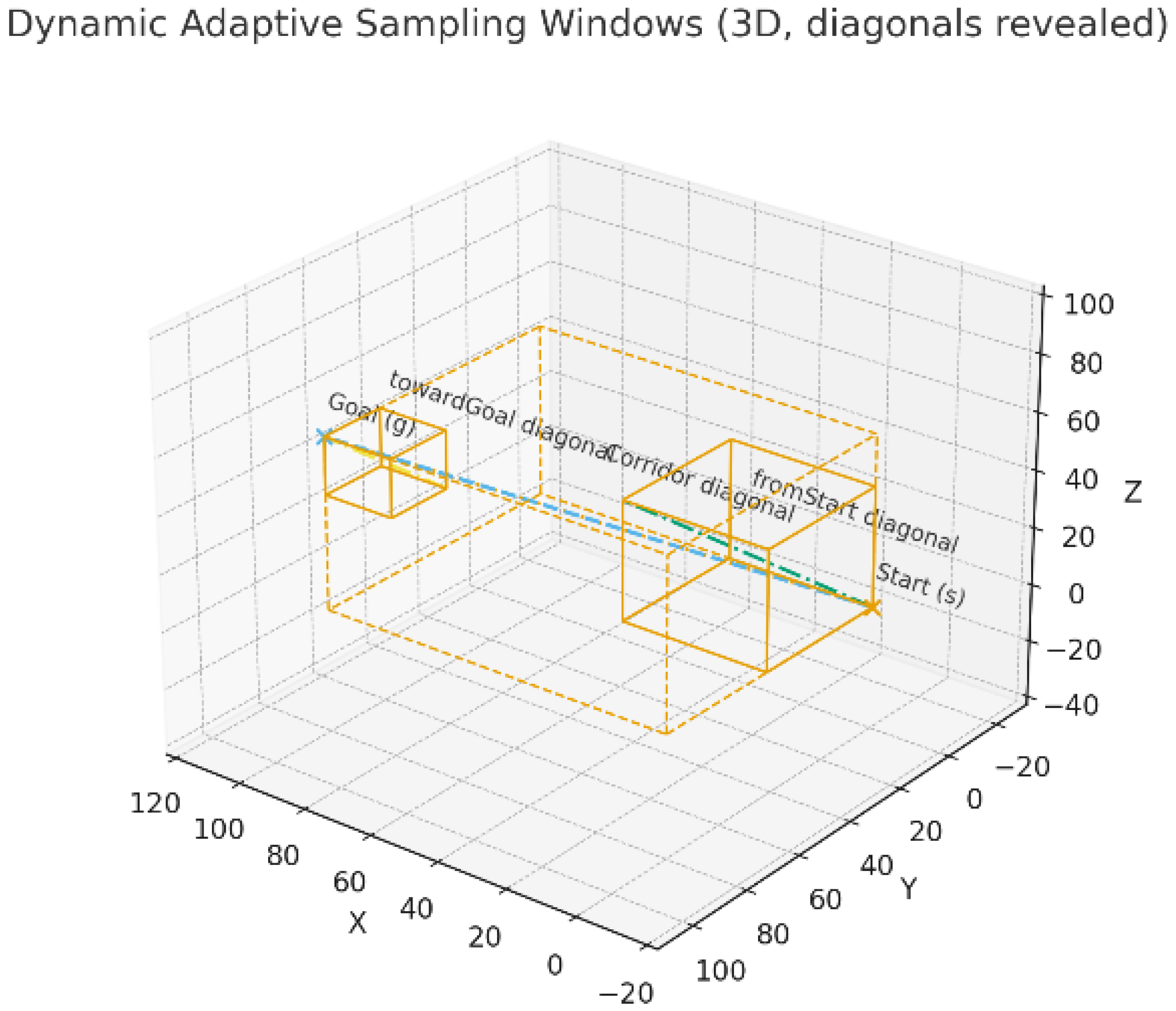
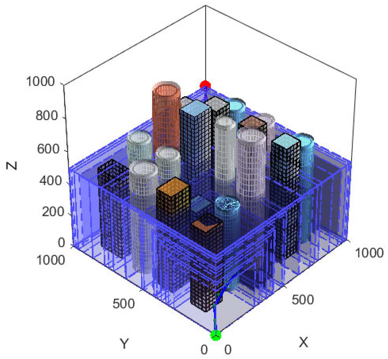
The sampling space diagram is shown in the figure below. The workspace in Figure 3 is 120 × 120 × 100   m 3 (axes in meters). Start: ( 10 , 20 , 5 )   m ; goal: ( 100 , 80 , 10 )   m . Orange boxes: adaptive windows (initially 40 × 40 × 40   m 3 ) sliding along the start–goal corridor and shrinking according to Equation (4). The workspace in Figure 4 is a cubic region of X , Y , Z [ 0,1000 ]   m . Rectangular and cylindrical obstacles represent urban buildings, randomly distributed with base sizes between 50 and 150 m and heights ranging from 200 m to 800 m. The blue translucent box denotes the feasible free space dynamically adjusted during sampling (see Section 3.3). The green and red markers indicate the start and goal points, respectively. All coordinates are expressed in meters.

3.4. Hybrid Sampling

Traditional RRT uses pseudo-random sampling [22], which leads to sampling voids in some regions and redundant sampling in others. These deficiencies cause repeated exploration of certain areas and failed exploration elsewhere, slowing the algorithm’s convergence. To address this, within the dynamic adaptive sampling window, we propose a parallel hybrid of low-discrepancy Halton sampling and “bridge” (narrow-gap) sampling. In each iteration, candidate samples are generated: A proportion follows the Halton branch, while the remaining proportion follows the Bridge branch. The two candidate sets are merged and scored/ranked using a unified multi-objective cost J ( · ) ; the top candidates are then used to attempt one RRT* “extend + collision-check + rewire” step. This design simultaneously ensures coverage and corridor penetration, significantly reducing the time to the first feasible path in most scenarios and yielding more uniform, comprehensive path planning tailored to urban UAV models.

3.4.1. Halton Sampling

Halton sampling [23], thanks to its uniform coverage and low-discrepancy properties, generates a low-discrepancy sequence in the unit hypercube. With a finite number of samples, Halton sampling is closer to a “uniform distribution” than purely random sampling, yielding more stable coverage over large search domains. This paper adopts two refinements: (1) reduce sequence correlations via base scrambling and leapfrogging to improve robustness; (2) add slight jitter to balance low discrepancy with mild randomness, avoiding systematic striping near high-dimensional geometric boundaries. The following formula slightly perturbs the Halton point within the unit cube and then “scales/translates” it to the current sampling box, producing a realized sample.
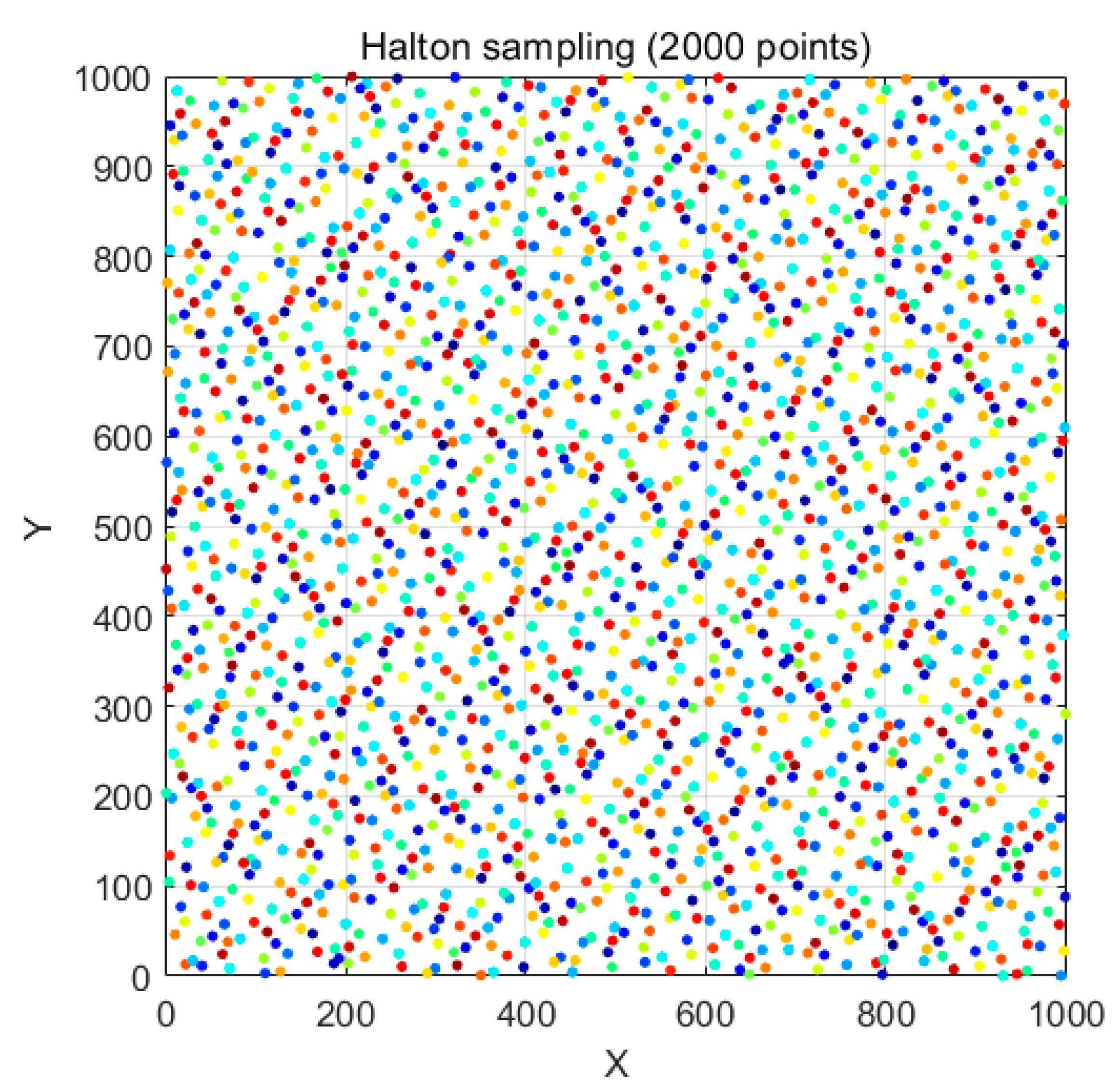
Compared with random sampling, the Halton branch is highly efficient in wide-open regions without narrow passages. Coupled with the EMA-smoothed dynamic window, it continually concentrates samples within the corridor that is most likely to yield a solution. The sampling comparison is shown in Figure 5 below. Figure 5 shows that a total of 2000 points were sampled uniformly on a horizontal plane. It highlights the significant variability of the random sequence—some areas have dense samples, while others have sparse samples. All coordinates are in meters. Figure 6 shows that points are generated using a low-discrepancy Halton sequence with prime bases (2,3), producing a quasi-uniform distribution with improved spatial homogeneity and reduced void regions.

3.4.2. Bridge Sampling

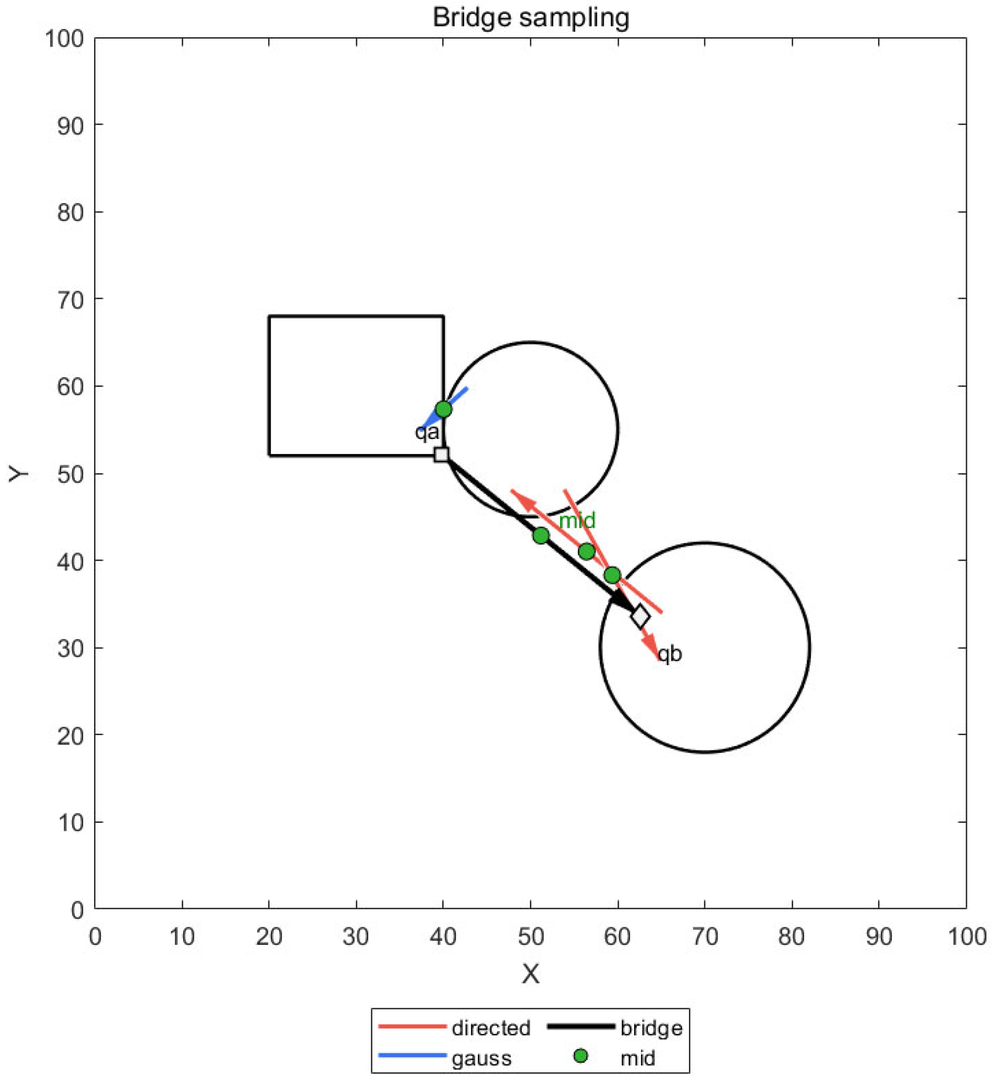
Unlike the Halton branch, the Bridge branch [24] samples by selecting two end points q a ,     q b on opposite sides of an obstacle, with their midpoint lying in free space. This midpoint typically lies near the obstacle’s medial axis, i.e., a high-value region within a narrow passage. We design a “midpoint test + endpoint generation” strategy for this branch.
During endpoint generation for the Bridge branch, we adopt three modes: directed extrapolation, undirected extrapolation, and a hybrid scheme.
Directed extrapolation: Randomly choose an obstacle and sample a point q a inside it. Push outward from the obstacle’s center in the centrifugal direction to obtain q b , and then perform the bridging sampling test again. Directed outward pushing can achieve a higher acceptance rate and more stable positioning when the obstacle shape is relatively regular.
Undirected extrapolation: Use the mean μ of the most recent failed midpoint and the obstacle center, draw a Gaussian sample around μ , and then extrapolate outward.
The two endpoints generated by the three Bridge-branch modes lie in free space around the obstacle midpoint, which can markedly improve the likelihood of a UAV passing through narrow urban corridors.
The bridge sampling schematic is shown in Figure 7 below. It shows the white circles denote the sampled endpoints q a , q b , the green dot in between is the midpoint that satisfies the criterion, the black segment represents the bridge, the red arrow indicates directed extrapolation, and the blue arrow indicates undirected extrapolation.

3.4.3. Multi-Objective Cost Ranking

The above sampling process supplies the planner with many expansion candidates, but naively iterating through them would lead to excessive, unproductive collision checks and low-quality attempts. Given the inherent trade-offs among objectives such as “proximity to the goal,” “obstacle clearance,” and “steering smoothness (or energy use/passability),” we introduce a multi-objective cost schedule after sampling. Concretely, we first unify units and normalize each metric, then combine them via weights into a composite cost function to rank and filter the candidate set. During expansion, candidates are tried in descending order of this schedule; once the first feasible candidate is found, we stop—reducing computation while tending to produce shorter, safer, and smoother local updates.
For the merging of the Halton branch and the Bridge branch, this paper proposes a multi-objective cost ranking J · . The two branch candidates are merged into the set Q = q , using the following multi-objective cost ranking. The formula is as follows:
J q = w g q g + w r e p ϕ ( d ( q ) ; d 0 ) + w c 1 m a x d q , ε + w h ( 1 c o s θ ( q ) )
Here, d ( q ) denotes the clearance, and ϕ ( · ) takes the form of a smooth repulsive force such as m a x { 0 , ( 1 d d 0 ) 2 } . θ ( q ) represents the angle between the direction of the parent edge and the vector ( q q n e a r ) . The weights w g , w r e p , w c , w h respectively reflect the trade-offs among target attraction, obstacle avoidance, safety distance, and heading smoothness. w g encourages sampled points to approach the sub-goal; w r e p , w c jointly encourage keeping clearance while avoiding sticking too close to obstacles; w h reduces backtracking samples, guiding the UAV to sample along the forward direction.

3.5. Target Bias Expansion Strategy

In sampling-based planners (RRT* and its bidirectional variants), biasing samples toward the goal can significantly reduce the time to the first feasible path. However, a fixed bias can become overly optimistic or lead to reckless, straight-line attempts in complex environments—especially those with narrow gaps or dense obstacles. To address this, we propose an adaptive goal bias based on recent statistics: when “straight-to-goal” attempts show higher success rates within a recent window, we increase the proportion of goal-directed samples; when attempts repeatedly fail, we reduce the bias and switch to frustum-cone sampling to skirt obstacles. If both strategies fail, we fall back to a safeguard of purely random expansion.

3.5.1. Adaptive Target Bias Model

The proposed adaptive goal bias [25] computes a sliding-window success rate before goal-directed sampling, and then—based on that rate—uses one of two goal-bias expansion strategies with a certain probability. We set upper and lower bounds on this probability to avoid extremes. With this auto-tuned probability, each of the two trees independently makes dynamic trade-offs, so that goal-directed samples are less likely to be trapped by obstacles.
In each goal-biased round, we first attempt a straight-to-goal expansion. If a feasible segment is found, we record a success; otherwise, it is marked as a failure—though if the straight-to-goal attempt was not used in that round, no mark is needed. After marking each round, we use the recent history of marks to set the probability for the next round. To prevent extreme values, we bound this probability by 0 < p m i n < p m a x < 1 . The start-tree and goal-tree probabilities are independent and do not interfere with each other. To handle varying terrain conditions, we introduce a terrain parameter γ to aid probability tuning: for concave or conservative terrain, set γ > 1 ; in open areas, set γ < 1 . This design helps modulate the sensitivity of the probability. Let the window length be W , and let the number of valid samples in the most recent window be m t [ 1 , W ] . The success rate s t is defined by the following formula:
s t = 1 m t j I t a j , s t [ 0,1 ]
p g , t = p m i n + ( p m a x p m i n ) s t γ [ p m i n , p m a x ]
s t = 0 p g , t = p m i n
s t = 1 p g , t = p m a x
Formula (6) defines the calculation method for s t . The value of a j depends on the outcome of each round of target bias: 1 if successful, 0 otherwise. Formula (7) sets the upper and lower bounds for the success rate, while Formulas (8) and (10) correspond to the boundary calculations for the success rate.

3.5.2. Direct Pointing Extension

Straight-to-goal expansion [26] means that in each expansion round, we prioritize—with a certain probability—extending directly toward the goal (or toward the frontier node of the opposite tree), rather than performing a standard random expansion. The core aim is to rapidly shrink the distance to the goal or the opposite tree and complete the connection as early as possible, while gracefully falling back to a more robust exploration mode when attempts fail. The specific steps of straight-to-goal expansion are as follows:
Step 1. Select the parent node: In the current tree, choose the node most conducive to approaching the goal—the node closest to the goal.
Step 2. Calculate step size: Extend a small step from the parent node in the direction “pointing toward the target,” with the step size not exceeding the set expansion step size.
Step 3. Determination and Update: When the newly inserted node satisfies the path requirement, update the tree structure; when it does not satisfy the path requirement, switch to the cross-sectional cone candidate sampling expansion.
Typically, when facing open terrain, drones achieve greater efficiency with direct-pointing extended sampling, offering faster convergence and enhanced stability. However, urban environments are generally complex and feature numerous obstacles, making subsequent cross-sectional cone sampling a more suitable approach.

3.5.3. Cross-Sectional Conical Sampling Extension

When “Directed Goal-Seeking” expansion fails, immediately reverting to global random expansion causes efficiency to plummet. The idea behind sectional cone candidate sampling is to maintain the overall “toward-target” direction while selecting several “more promising” candidate points within a local sector (conical shell) around that direction. These points are then connected in order of multi-objective cost from best to worst. This approach avoids minor protrusions/edges of nearby obstacles without losing the global tendency to “rapidly approach the target.” The sectional cone sampling expansion samples candidates within an axis-aligned sectional cone centered at q n g and oriented along the u —axis. After scoring candidates based on proximity to the target, distance from obstacles, and minimal turning angle, segment tests are performed sequentially. The first feasible expansion is adopted. The specific implementation of sectional cone candidate sampling expansion is detailed below.
Step 1. Determine the axis: Using the parent node to be expanded as the vertex, take the direction pointing toward the global target as the central axis of the cone.
Step 2. Establish section coordinates: Select any two unit vectors perpendicular to the axis as the coordinate axes e 1 , e 2 of the conical section, which are mutually orthogonal to the central axis.
Step 3. Set geometric dimensions: Height shall not exceed twice the tree height nor exceed the straight-line distance from the parent node to the target; bottom radius is typically 1–2.5 times the step length; lower section segment position is set at half the height; opening size increases linearly with height.
Step 4. Distribute points uniformly within the cross-sectional cone: Take samples inside the cone, ensuring the sampling remains as uniform as possible in terms of volume.
Step 5. Basic Filtering: Directly eliminate candidates that extend beyond the workspace boundaries or fall within obstacles.
Step 6. Candidate Scoring and Ranking: Each candidate point is scored based on its distance from the target point, distance from obstacles, and steering angle. Points are assigned comprehensively. Points are better, ranking higher, and extending stride length earlier.
Step 7. Sequential Line Connection: Starting from the candidate with the highest score, extend a new point along its direction by only one step length. Perform a segment feasibility check (no collision and within boundaries). Accept and connect to the tree upon encountering the first feasible candidate. If all attempts fail, determine that this round of cone candidates is unsuccessful and revert to the random strategy.
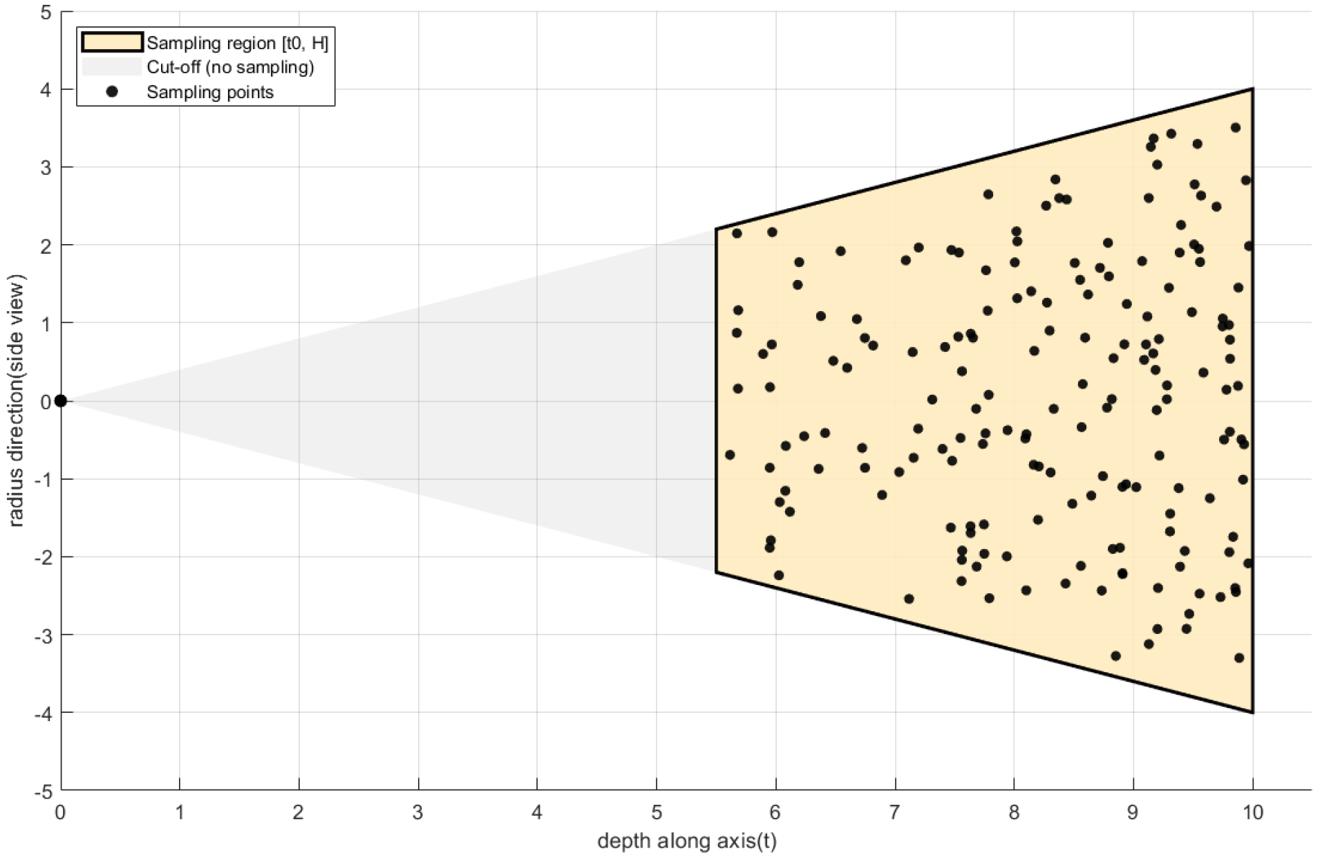
The cross-sectional cone sampling is shown in the Figure 8 below. The local sampling region is a truncated cone with an axial depth of L = 10   m , an entrance radius of r 1 = 1   m , and an exit radius of r 2 = 4   m , corresponding to a half-angle of approximately 12.6 . Black dots denote 200 randomly generated candidate points within the cone cross-section, used for local extension during the adaptive expansion process. The gray area indicates the feasible sampling corridor along the forward direction of the current node. Axes are expressed in meters.
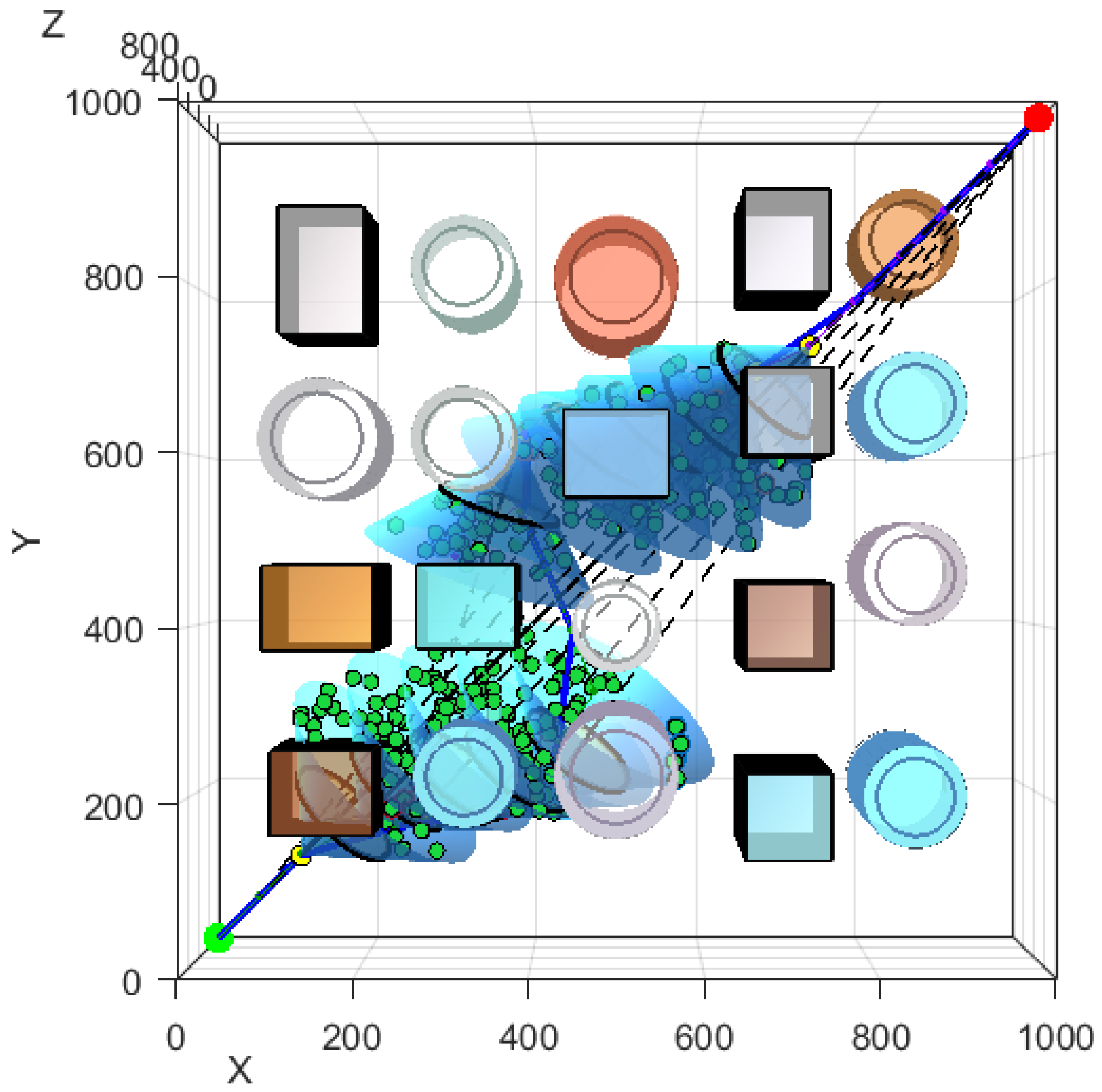
Another picture (Figure 9) illustrates multiple bidirectional cross-sectional cone sampling between target points under urban modeling conditions. The global environment is defined as X , Y , Z = 1000 , 1000 , 800   m , containing multiple cuboid obstacles representing buildings with heights of 200–600 m. Blue translucent clusters represent the feasible sampled points within successive truncated-cone regions generated along the expanding branch of the tree. The start and goal positions are shown by the green and red spheres, respectively. The adaptive cone parameters are L = 80   m , r 1 = 10   m , r 2 = 50   m ; All coordinates are expressed in meters.
Direct pointing expansion is the fastest and most aggressive, but has the poorest obstacle avoidance performance. Cross-sectional conical candidate sampling expansion can directly bypass obstacles while maintaining obstacle avoidance capabilities on top of straight-line expansion. However, both methods are easily blocked by large obstacles. Furthermore, they remain goal-oriented and cannot achieve full spatial coverage. Therefore, random expansion is required as a fallback to ensure an infinite number of iterations will eventually find a path. Coordinating these three methods enables both rapid pathfinding and improved obstacle avoidance.

3.6. Multi-Objective Path Optimization

Although path expansion enables rapid generation of feasible paths in complex 3D environments, the initial solution often suffers from redundant detours, jagged turns, insufficient clearance, and may fail to meet practical system requirements for velocity/acceleration continuity. To address this, this paper introduces a two-stage “planning-optimization” process after path expansion: First, within the start/end corridor constraints, particle swarm optimization (PSO) performs global fine-tuning of internal waypoints along the discrete trajectory, balancing the composite objectives of “minimum length, collision penalty, obstacle clearance, and second-order smoothness.” Subsequently, distance-threshold-driven interpolation refinement and cubic B -spline smoothing re-parameterization convert the discrete polygon into a C 2 -continuous executable trajectory, with safety re-evaluation performed on the spline. Experiments demonstrate that this two-stage strategy significantly shortens path length, increases minimum clearance, reduces maximum turning angle, and enhances trajectory dynamic trackability without compromising feasibility.

3.6.1. Multi-Objective Path Optimization Modeling

Given an initial discrete path, output a feasible polyline P = [ P 1 , P 2 , , P n ] , where only the intermediate control points P 2 , , P n 1 are optimized. In the three-dimensional state, the path is unfolded in sequence into decision variables and stacked as x = v e c ( P 2 , , P n 1 ) R 3 ( n 2 ) , with the endpoints P 1   and P n kept fixed. Each dimension is bounded by constraints x [ l , u ] R ( n 2 ) .
A multi-objective function is defined with the combined goals of minimum path length, collision penalty, obstacle clearance, and second-order smoothness, expressed as follows Formula (10):
J x = w L i = 1 n 1 p ~ i + 1 p ~ i + w C t = 1 n 1 1 c o l l p ~ i , p ~ i + 1 · C c o l l +   w S λ S i = 1 n 1 ψ ( d m i n ( P ¯ i , P ¯ i + 1 ) ) + w S m κ i = 2 n 1 p ~ i 1 2 p ~ i + p ~ i + 1 2
where p ~ i + 1 p ~ i denotes the Euclidean distance between adjacent points; the indicator 1 coll = 1 means that the segment [ p ~ i , p ~ i + 1 ] intersects with an obstacle, and the penalty coefficient C coll is set much larger than 1; the function d m i n ( · ) represents the minimum external distance from a segment to an obstacle; the soft constraint potential function for the minimum safety distance is defined as ψ ( d ) = λ s m a x { 0 , d 0 d } 2 ; κ is the smoothness scale; p ~ i 1 2 p ~ i + p ~ i + 1 2   is the second-order difference smoothing term, equivalent to a discrete regularization of curvature. This suppresses sharp corners and high-frequency oscillations while providing a good initial value for subsequent spline fitting. The overall multi-objective function promotes a trend toward continuous optimization while retaining strong penalties for rigid safety constraints.

3.6.2. PSO Optimization Path

Particle Swarm Optimization (PSO) is an evolutionary computation method based on swarm intelligence. It uses the behavior of hummingbirds as a model, simulating the process of a flock of birds searching for food to solve complex optimization problems, which can effectively improve computing efficiency and accuracy. The basic idea of PSO is to regard the optimization problem within the feasible domain as a set of particles, where each particle represents a potential optimal solution. These particles move through the solution space according to certain rules, and through iterative updates, they eventually converge to one or more optimal solutions.
Based on the standard PSO algorithm, this paper improves the process of searching for the optimal solution with the following modifications:
  • In the standard PSO, the individual learning factor, social learning factor, and inertia weight are fixed. In this work, success rate and population diversity are introduced as feedback to adaptively adjust the solving speed of the PSO algorithm online.
  • When stagnation in the search for the optimal solution is detected, a subset of particles is randomly selected and redirected to continue exploring for the optimum.
  • During the particle search process, once an obstacle is encountered, it is immediately marked to prevent repeated searches in the same region.
Improved PSO steps are as follows:
Step 1. Set the swarm size M , Initialize particle positions by applying small random perturbations or tangential adjustments to the original polyline; initialize velocities to 0.
Step 2. Compute the objective value J ( x p t ) for each particle, and update the Optimal individual and global optimality. The position and velocity of the p -th particle in generation t are denoted by ( x p t , v p t ) , optimal individual is represented by ( p B p t , f B p t ) , global optimality is represented by ( g B t , g f t ) .
Step 3. Introduce feedback signals
  s t = 1 M p = 1 M 1 { J ( x p t + 1 ) < f B p t } ,   d t = 1 d j = 1 d s t d ( { x p , j t + 1 } p = 1 M ) m a x ( u j l j , ε ) [ 0 , )
s t reflects whether the particles are gradually improving during the search process, while d t reflects whether the particles are overly crowded or too dispersed.
Step 4. Modify the inertia weight and learning factors for the next generation. The specific update Formulas (11)–(14) are as follows:
e S = s * s t , e D = d * d t
ω t + 1 = c l i p ( ω t + a ω e D + b ω e S ,   [ ω m i n , ω m a x ] )
c t + 1 = c l i p ( c t + α c ( e D + e S ) , [ c 1 , m i n , c 1 , m a x ] )
c 2 , t + 1 = c l i p ( c 2 , t α 2 ( e D + e S ) , [ c 2 , m i n , c 2 , m a x ] )
At the same time, a state-driven mechanism is introduced in the improved algorithm, so that when a particle encounters an obstacle, it can immediately return to the exploration state.
Step 5. Particle velocity update:
v p t + 1 = ω t v p t + c 1 , t r 1 ( p B p t x p t ) + c 2 , t r 2 ( g B t x p t )
Step 6. Particle position update
x p t + 1 = c l i p ( x p t + v p t + 1 , l , u )
where r 1 , r 2 ~ U ( [ 0,1 ] d ) , denotes the Hadamard (element-wise) product, c l i p enforces the boundary constraints.
Step 7. When the generation limit or a relative improvement criterion is reached, output the best discrete path.
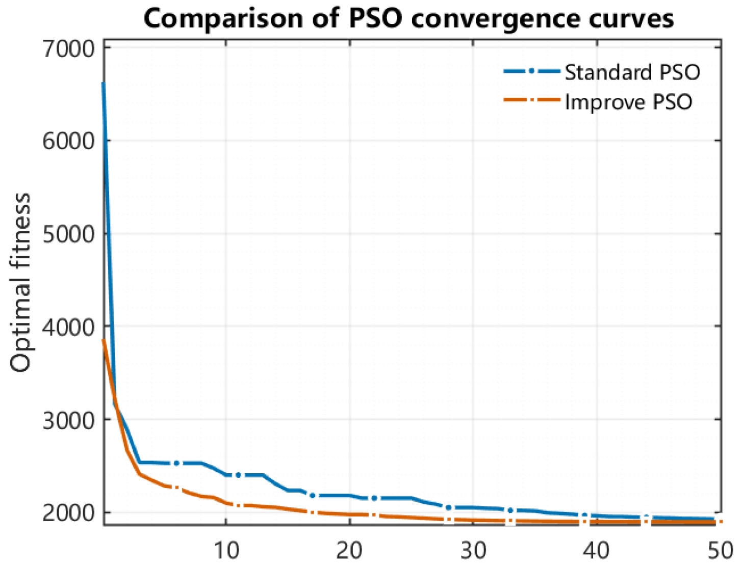
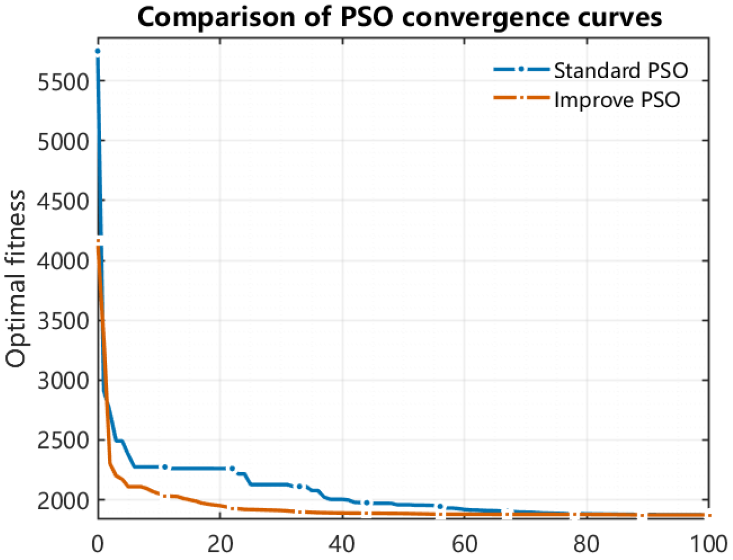
Figure 10 shows the convergence curve of PSO within 50 iterations: the dashed line represents the standard PSO, and the dash-dotted line represents the improved PSO. The vertical axis denotes the best fitness (objective function value), where lower values are better. The horizontal axis represents the number of iterations, the inertia weight decreases linearly from 0.9 to 0.4, and the cognitive and social coefficients are set as c 1 = c 2 = 2.0 . The improved PSO integrates an adaptive feedback mechanism to dynamically adjust inertia weight based on swarm diversity. The fitness value corresponds to the multi-objective cost defined in Equation (10). Figure 11 presents the convergence comparison under the same experimental setup for 100 iterations. Experimental setup is identical to that in Figure 10. Both figures adopt the same initialization and parameter ranges. The improved PSO converges faster, achieves lower final values, and exhibits a smoother process. The horizontal axis represents the number of iterations.
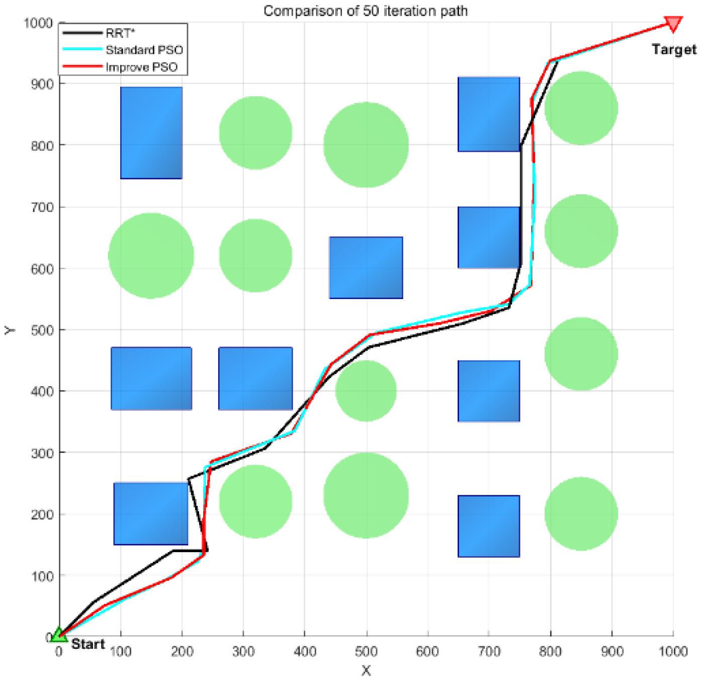
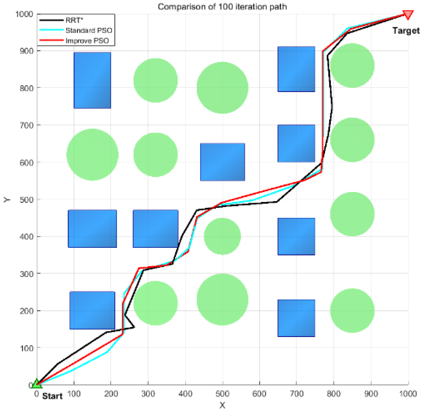
Based on the improved PSO algorithm, we generated path plots for RRT*, standard PSO, and improved PSO under 50 and 100 iterations, as shown in Figure 12 and Figure 13. It compares the planar paths obtained by the three algorithms after 50 iterations in the same obstacle environment: RRT* (black), standard PSO (blue), and improved PSO (red). The global environment is defined as X , Y , = 1000 , 1000   m . The start point is located at the lower-left corner and the goal at the upper-right corner; green circles and blue rectangles denote obstacles. It uses the same settings as Figure 13, but with 100 iterations. The red path is overall shorter and smoother, while maintaining a larger safety margin around obstacles.
These results demonstrate that, under the same iteration budget, the improved PSO converges faster, produces shorter and smoother paths, and preserves larger safety margins near obstacles. As the number of iterations increases, the standard PSO gradually approaches the improved performance, but still exhibits sharp turns in certain bottleneck segments. RRT* provides a reliable feasible initial solution, but is inferior in terms of final path quality and smoothness.

3.6.3. Interpolation Optimization Path

The PSO path optimization has already shortened the discrete polyline, increased clearance from obstacles, and reduced turning angles. However, the resulting path is still not suitable for UAV flight in urban environments due to its insufficient sampling density and lack of continuity, which hinder UAV control and tracking. Therefore, on top of Improved PSO algorithm, a two-step interpolation optimization is applied:
(1)
Apply linear interpolation with a distance threshold to densify long segments (gap-filling), thereby improving geometric resolution and the reliability of safety evaluation.
(2)
Use a cubic B-spline to smooth and re-parameterize the densified polyline, producing a C 2 -continuous executable trajectory, followed by a secondary safety check along the spline.
The interpolation optimization procedure is as follows:
Step 1. Interpolation densification.
The long segments of the polyline output by PSO are densified according to a “length threshold.” Let the PSO output polyline be P = p 1 , , p n , p i R 3 . For the i-th segment, compute its length   L i = P i + 1 P i . Given a threshold d m a x , the following rule is applied:
If L i d m a x ,   keep the segment unchanged;
If L i > d m a x , insert k i interpolation points within the interval, with parameters t i j , generating interpolated points p i , j . This produces the densified path P ~ .
When choosing d m a x , factors such as collision detection step size, control frequency, and maximum velocity must be considered. Linear interpolation densification with a distance threshold ensures that dense detection points are added within long segments, leading to more reliable safety evaluation, more uniform knot distribution for subsequent spline fitting, improved stability, and reduced sharp corners.
Step 2. Cubic B-spline smoothing.
Each of the three components x , y , z is fitted separately into a continuous curve using a cubic B-spline. For segments close to obstacles, hard interpolation is applied to ensure that clearance margins are not “smoothed out.” For other segments, a least-squares fit with light regularization is used to obtain a smooth shape. This yields a continuous, time-parameterizable trajectory curve. The cubic B-spline is expressed as Formula (17):
C ( u ) = j N j , 3 ( u ) P j , u [ 0,1 ]
where N j , 3 is the cubic basis function and P j   are the control points. Chord-length parameterization is used to assign u , with endpoint clamping applied at both ends.
Step 3. Post-smoothing collision check.
A fixed-step collision check is performed along the spline curve. After obtaining the smoothed trajectory, each segment is inspected; if local obstacle penetration is detected, the smoothing weight of that segment is reduced. This ensures that the final trajectory maintains both smoothness and accuracy.
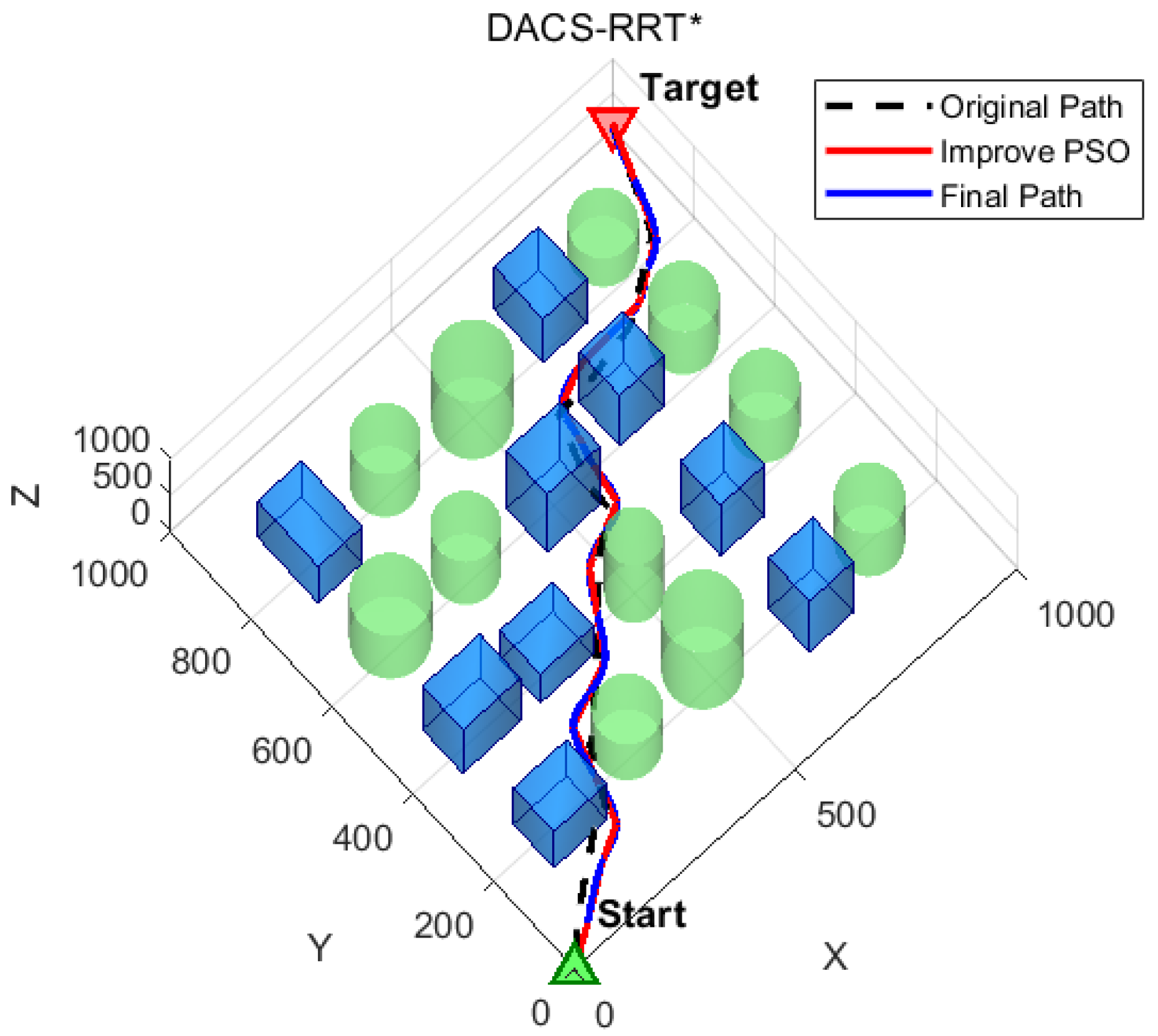
Figure 14 shows a comparison of DACS paths. The global environment is defined as X , Y , Z = 1000 , 1000 , 1000   m Green cylinders and blue cubes represent obstacles; the black dashed line indicates the original feasible polyline generated by RRT*; the red line shows the polyline optimized by PSO; and the blue line represents the final smoothed trajectory (cubic B-spline with secondary safety recheck). The start point is located at the lower left and the target at the upper right.
The “interpolation densification + cubic B-spline” post-processing upgrades the discrete polyline generated by PSO into a continuous, clearance-sufficient, and time-parameterizable executable trajectory without sacrificing feasibility. By applying a segment-length threshold and adaptive resolution control, it significantly reduces the risk of “leap-over” missed detections. The cubic B-spline employs chord-length parameterization with endpoint clamping, using “hard interpolation” near obstacles and “least-squares + regularization” fitting elsewhere to balance safety and smoothness. A secondary safety recheck and local rollback strategy ensure that the final trajectory maintains the same level of safety as the original feasible path. Experimental results demonstrate that this post-processing consistently reduces maximum turning angles and curvature, maintains or shortens total path length, and improves both minimum clearance and tracking smoothness.

3.7. Theoretical Properties and Analytical Discussion

The proposed DACS-RRT* algorithm is an adaptive extension of the classical RRT* framework. While RRT* has been mathematically proven to be probabilistically complete and asymptotically optimal [27], the dynamic and adaptive modifications introduced here—namely, (1) dynamic adjustment of sampling space, (2) hybrid Halton–Bridge sampling, and (3) adaptive goal-bias and conical expansion—necessitate an analytical discussion to confirm that these theoretical properties are preserved.
(1)
Probabilistic completeness.
RRT* achieves probabilistic completeness because its sampling process covers the entire free configuration space X f r e e with nonzero probability. In DACS-RRT*, although the sampling region dynamically adjusts, it always remains a subset of X f r e e that gradually shifts toward the goal while maintaining coverage of feasible corridors. The Halton–Bridge hybrid sampling still ensures that every region of X f r e e retains a nonzero probability of being sampled. Therefore, given infinite iterations n , the probability that DACS-RRT* finds a feasible path, if one exists, converges to one.
(2)
Asymptotic optimality.
Asymptotic optimality of RRT* follows from its rewiring mechanism, which ensures that the cost of the best path monotonically decreases and converges to the global optimum. DACS-RRT* preserves the same rewiring principle and cost-update rule. Under the same assumptions as RRT*, the adaptive expansion only modifies how new nodes are proposed, not how connections are optimized. The multi-objective local ranking merely biases sampling toward high-quality candidates, accelerating convergence without changing the underlying optimality property.
(3)
Convergence characteristics.
The dynamic sampling window and adaptive goal-bias control influence convergence speed but not convergence direction or guarantee. Empirical evidence (Section 4) confirms that convergence is significantly faster than standard RRT*, and the variance of planning time remains extremely low. Theoretically, since each adaptive rule is bounded and reversible (expansion can always revert to uniform random sampling), the Markov chain of node generation remains ergodic over X f r e e , satisfying the sufficient condition for convergence to a globally optimal tree.
While a rigorous mathematical proof is beyond the present scope, the above analysis shows that DACS-RRT* satisfies the same sufficient conditions for probabilistic completeness and asymptotic optimality as RRT*. The introduced adaptive mechanisms modify the sampling efficiency rather than the reachability or rewiring principles, thus maintaining the theoretical properties of the base algorithm.

4. Analysis and Verification of the Dynamic Adaptive RRT* Algorithm

4.1. Parameter Settings and Fairness of Comparison

To ensure a fair comparison, all baseline algorithms (RRT*, RRT-Connect, GB-RRT*, BI-RRT*, and BAI-RRT*) were implemented using consistent frameworks and parameter initialization. The step size, neighbor radius, maximum iteration limit, and collision-check resolution were identical across all algorithms.
Each algorithm’s key hyperparameters (e.g., goal bias, step size multiplier, informed sampling radius) were tuned through grid search to achieve near-optimal performance under the same environment. For instance, the goal bias of GB-RRT* and BAI-RRT* was tested in the range [0.1, 0.4], and the value yielding the shortest average path length across three trials was selected. The same tuning protocol was applied to DACS-RRT*, ensuring no method was unfairly advantaged.
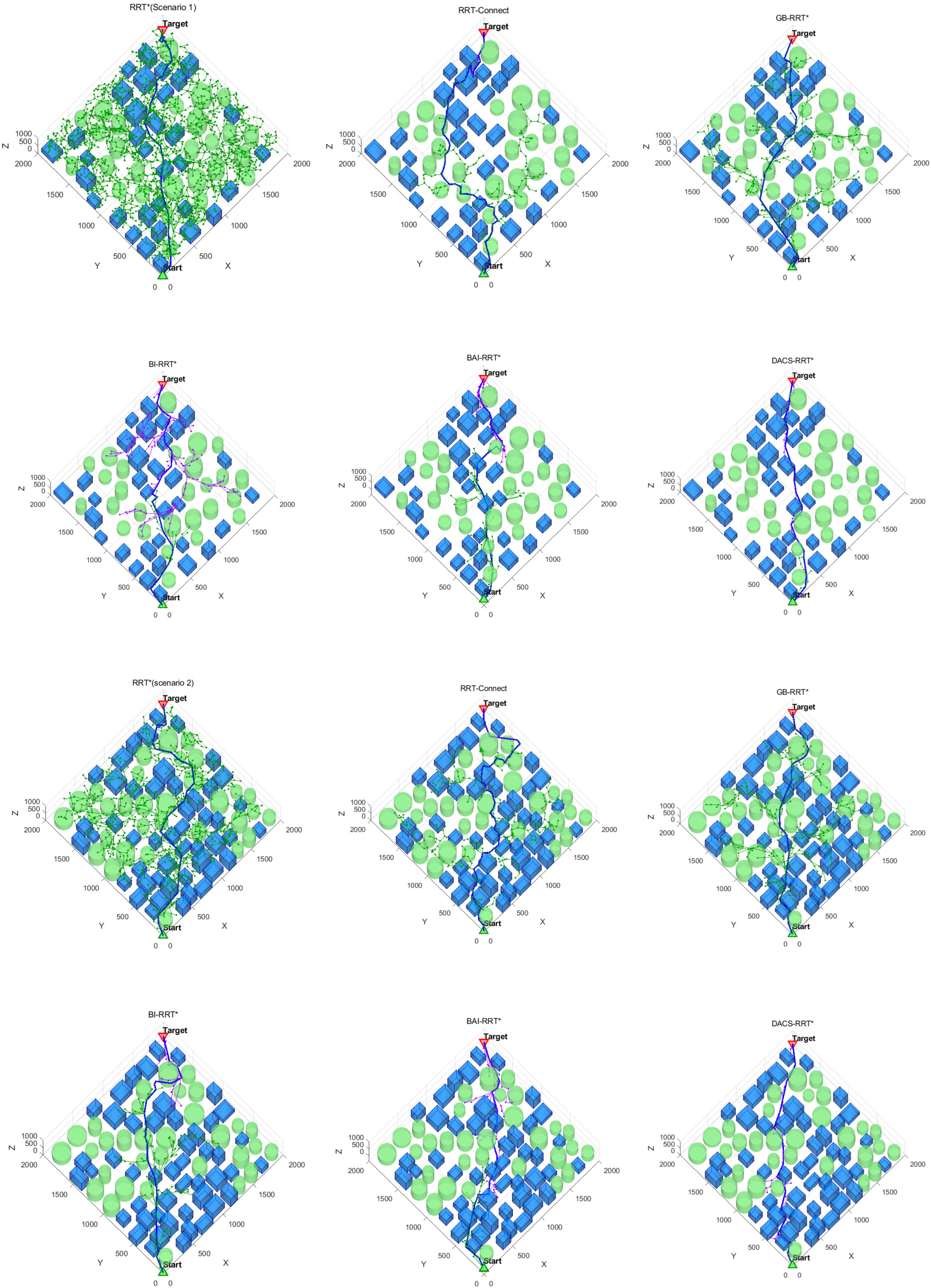
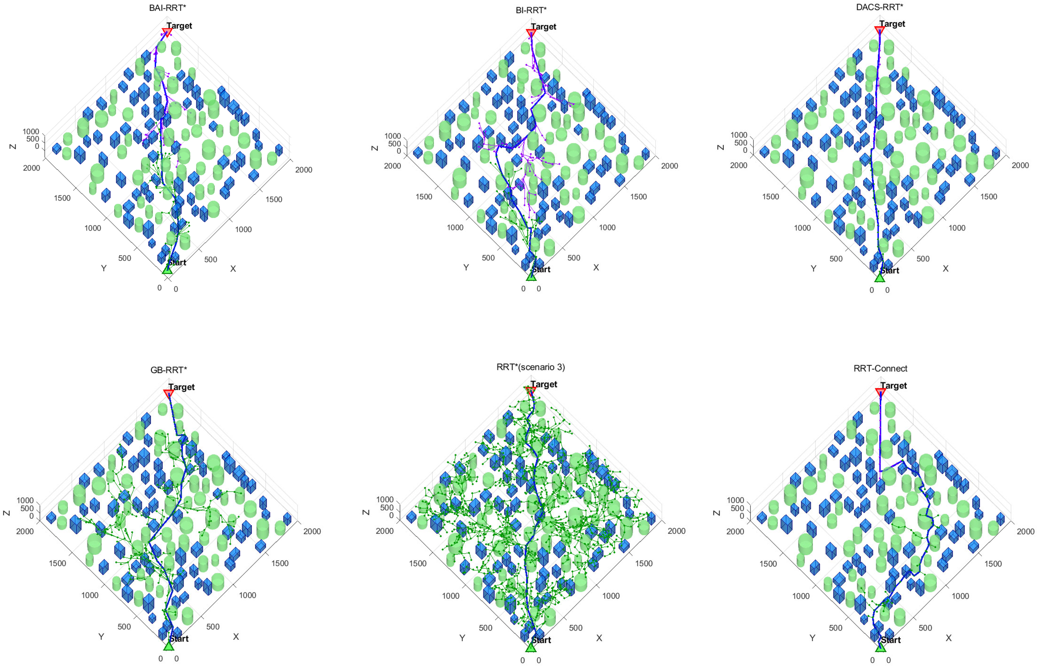
This study provides a comparative analysis between five baseline algorithms—RRT*, RRT-Connect, GB-RRT*, BI-RRT*, and BAI-RRT*—and the proposed DACS-RRT* algorithm. MATLAB 2024a was used as the software platform, and three different urban modeling scenarios were designed for evaluation:
Scenario 1: Moderate number of obstacles with medium density.
Scenario 2: Moderate number of obstacles with increased density.
Scenario 3: Increased number of obstacles with medium density.
We use procedurally generated urban blocks to control obstacle density, corridor width (narrow-passage presence), and height heterogeneity across three difficulty levels (sparse → medium → dense). This ensures paired, reproducible comparisons under identical budgets for all planners. In all three scenarios, the UAV takes off from the green-marked starting point and lands at a red-marked target point, navigating through clusters of urban buildings. For each algorithm—RRT*, RRT-Connect, GB-RRT*, BI-RRT*, BAI-RRT*, and the proposed DACS-RRT*—independent runs were performed 200 times in each scenario. Performance metrics were calculated as the average of the best 20 runs to reduce the impact of random error.
Notes on baseline algorithms:
RRT* is a Rapidly Expanding Random Tree algorithm that incorporates parent node policies. RRT-connect is a bidirectional Rapidly Expanding Random Tree algorithm. GB-RRT* is a goal-biased Rapidly Expanding Random Tree algorithm. BI-RRT* is a bidirectional informed Rapidly Expanding Random Tree algorithm. BAI-RRT* is a bidirectional adaptive informed Rapidly Expanding Random Tree algorithm.
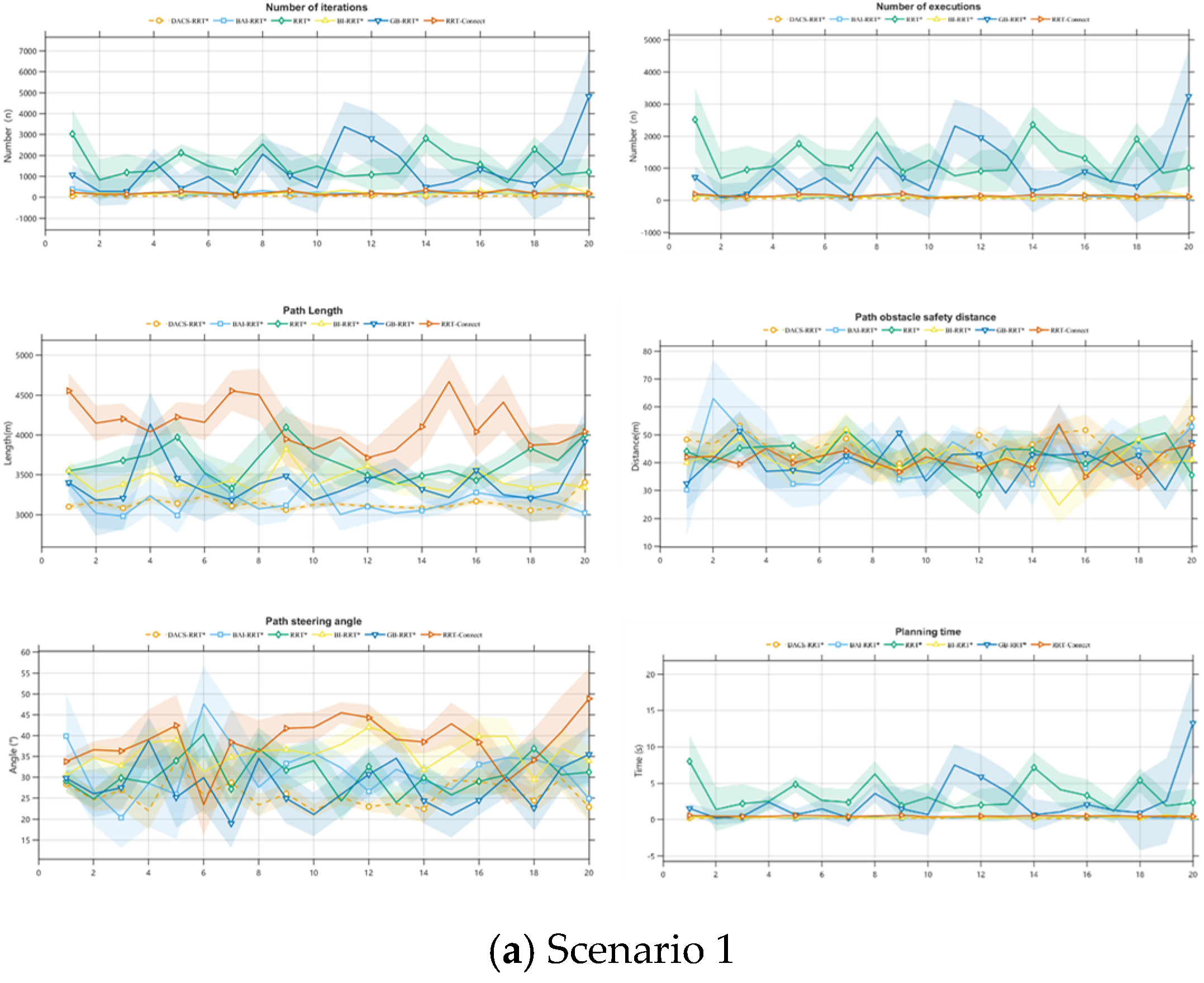
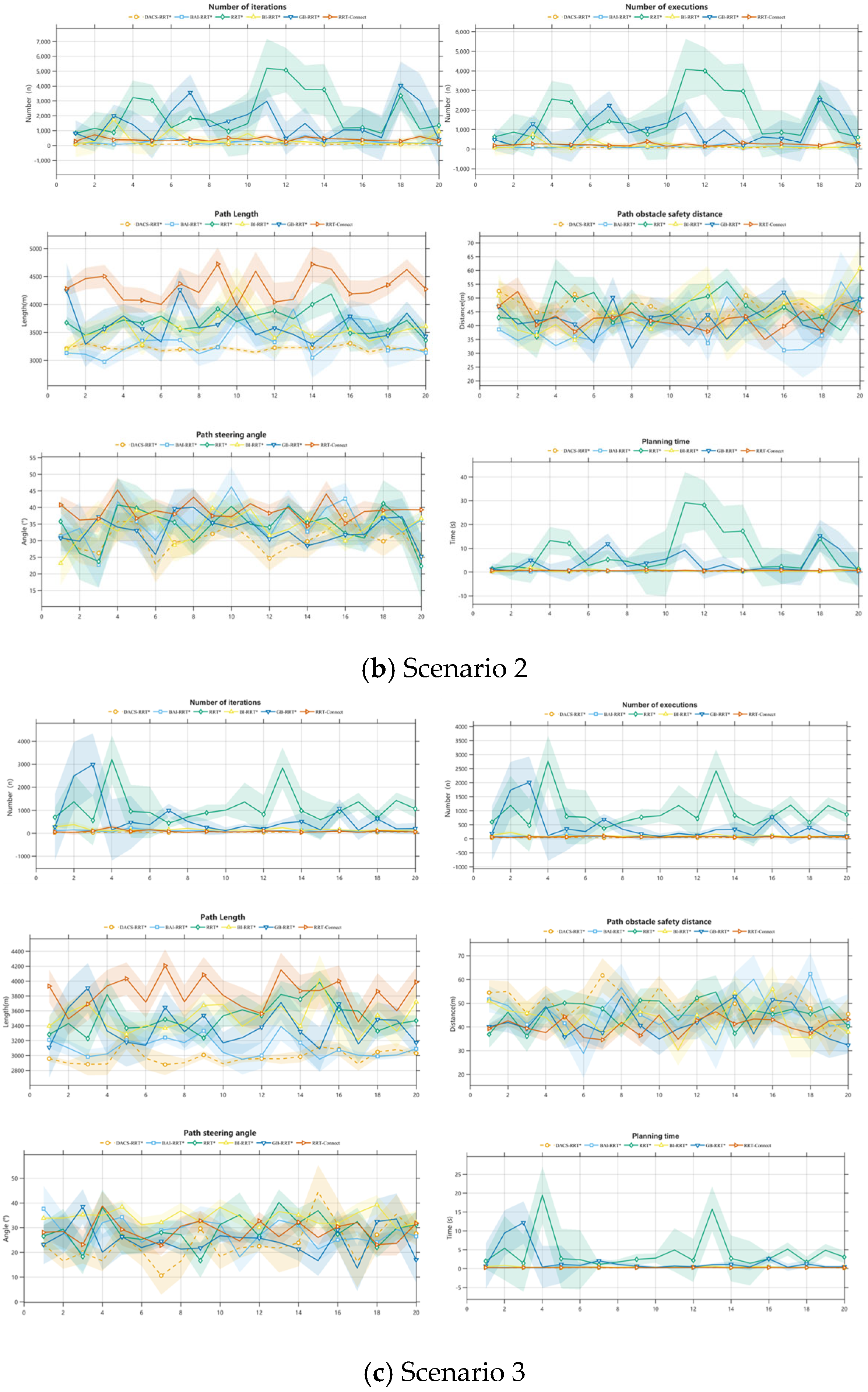
In the three randomized complex scenarios, we conducted 20 independent repeated experiments for all six algorithms (RRT*, RRT-Connect, GB-RRT*, BI-RRT*, BAI-RRT*, and DACS-RRT*), measuring planning time, path length, node count, iterations, average clearance distance, and average turning angle.

4.2. Computational Complexity Analysis

The computational complexity of RRT*-based algorithms primarily depends on the number of nodes n and the nearest-neighbor search process. For a uniform sampling distribution, the standard RRT* exhibits an average-case time complexity of: O ( n l o g n ) , due to the use of incremental nearest-neighbor queries and rewiring steps.
For the proposed DACS-RRT*, the dynamic sampling window and hybrid sampling introduce a constant-factor overhead in each iteration, but do not change the overall order of complexity. The adaptive selection of candidate samples (Halton–Bridge mixture) increases per-iteration computation by O ( k ) , where k is the number of candidates (typically ≤ 20). Hence, the total complexity remains: O ( k n l o g n ) O ( n l o g n ) , which is asymptotically equivalent to RRT*, with only a small constant-factor increase.
According to the experimental data in Section 4.3, the average time per iteration of DACS-RRT* is measured at 0.0046 s, while the standard RRT* is 0.0042 s, indicating that the adaptive operation improves convergence efficiency without significant computational overhead.

4.3. Experimental Results Analysis

From the overall cross-scenario results, DACS-RRT* consistently outperformed others in terms of efficiency, path quality, and stability. Its average planning time was only 0.273 s, representing a 94.8% reduction compared with RRT* and 90.4% compared with GB-RRT*, and also outperforming RRT-Connect, BI-RRT*, and BAI-RRT* by 45.2%, 38.3%, and 18.8%, respectively.
In terms of path quality, the average path length of DACS-RRT* was 3111 m, which was 24.0% shorter than RRT-Connect and 14.1% shorter than RRT*. It also reduced path length by over 10% compared with GB-RRT* and BI-RRT*, demonstrating its capability to traverse feasible corridors with lower cost under complex obstacle constraints.
Alongside improvements in efficiency and path quality, resource consumption was significantly reduced: compared with RRT*, node count and iteration count decreased by 95.0% and 95.9%, respectively (by 91.5% and 94.3% relative to GB-RRT*). Substantial reductions were also observed when compared with RRT-Connect, BI-RRT*, and BAI-RRT*. This directly reflects the effective suppression of redundant exploration during the search process.
From a geometric and controllability perspective, DACS-RRT* also demonstrates advantages in both safety margins and trackability. On average, the obstacle clearance distance increased by 13.4%/10.0%/9.7% compared with RRT-Connect, BI-RRT*, and BAI-RRT*, respectively (and by 13.3% compared with GB-RRT*), leaving larger safety buffers without sacrificing efficiency. Meanwhile, the average turning angle was reduced by 24.7%/23.2%/15.8% relative to the above three algorithms, resulting in smoother curves and gentler control, which is beneficial for downstream trajectory tracking and energy management.
In terms of stability, the variance of planning time for DACS-RRT* across the three scenarios remained as low as 0.003–0.005, significantly below that of RRT* and GB-RRT*. Variances in path length, node count, and iteration count were also smaller. Over 50 runs, the polylines and shaded bands exhibited almost no sharp spikes, reflecting strong robustness and reproducibility against random initialization and local perturbations.
From an engineering application perspective, DACS-RRT* consistently compressed the average planning time below 0.35 s in all three complex environments, while significantly reducing memory and computational overhead. This indicates readiness for online replanning and deployment on embedded platforms, ensuring both real-time performance and resource efficiency. The low variance further implies lower cost for parameter transfer and scenario adaptation. Scenario-specific results reinforce these findings:
Scenario 1: DACS-RRT* achieved average values of 0.222 s/3137 m 55.8 nodes, while RRT* and GB-RRT* showed not only larger means but also significantly greater variances.
Scenario 2: All methods exhibited increased planning times, yet DACS-RRT* maintained the shortest time (0.305 s) and a relatively short path (3215 m). In contrast, the time variance of RRT* surged dramatically to 78.79.
Scenario 3: RRT-Connect tended to pass through narrow gaps with higher costs in long connections, producing an average path length 1.29× that of DACS-RRT*. Meanwhile, DACS-RRT* sustained superior performance with a planning time of 0.295 s, a path length of 2980 m, and a smaller turning angle of 23.56°.
Although the degree of improvement varied with obstacle distribution structures, the overall pattern of being “faster, shorter, more stable, and safer” remained consistently in favor of DACS-RRT*.
Figure 15 is a visual comparison of the six planners across the three types of environments. RRT* and its goal-biased variants exhibit significant exploration redundancy and path backtracking when facing concave boundaries and dead ends. RRT-Connect and BI-RRT* accelerate convergence, but generate sharp turns and wall-hugging segments in narrow passages. In contrast, DACS-RRT* consistently produces sparser and more directionally oriented tree structures across all three environments, resulting in fewer polyline segments, smoother corners, and a central-axis bias within long narrow corridors, enabling early deflection when passing through dead ends. Collectively, these characteristics highlight its enhanced robustness under complex geometric constraints and topological traps.
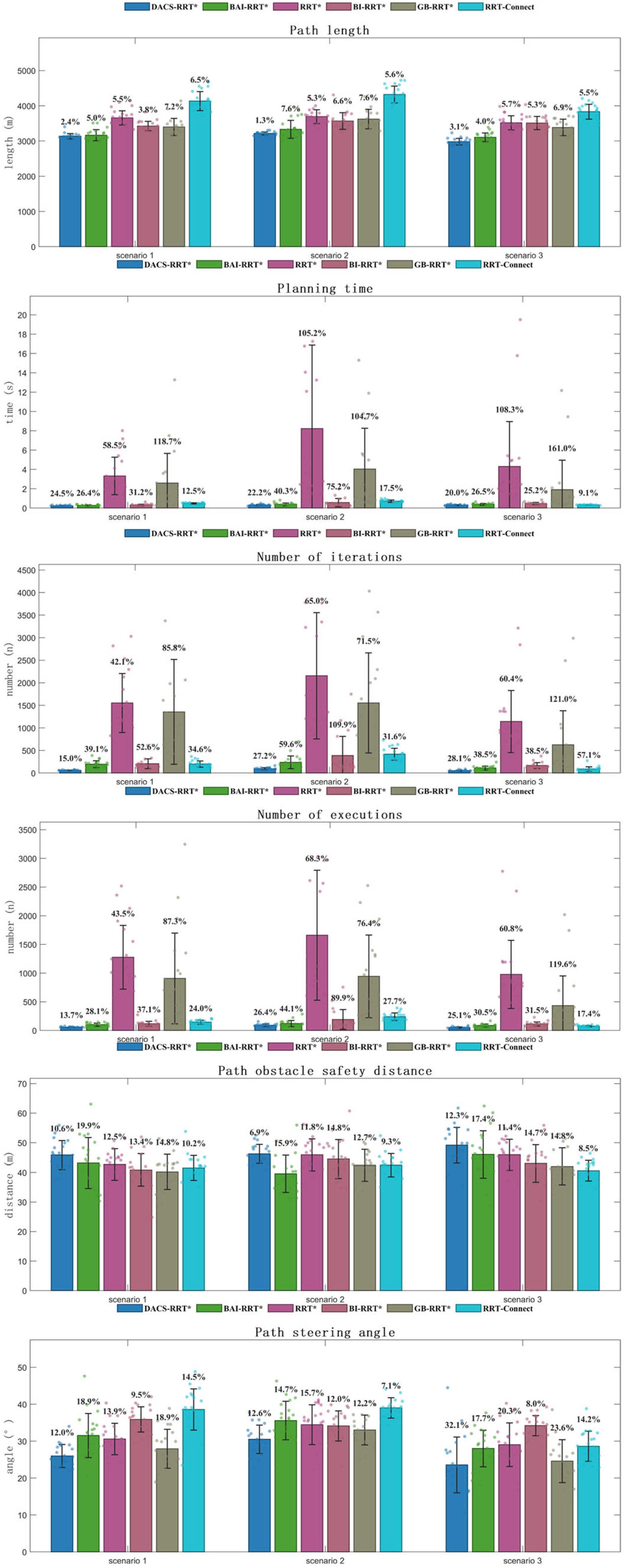
This paper presents line-plot comparisons of six performance metrics for six algorithms across the three scenarios (columns). As shown in Figure 16. The comparisons show that DACS-RRT* reaches stable low values earlier for quality metrics such as path length, clearance, and turning angle, while maintaining smaller peaks and smoother convergence trajectories in terms of node count and runtime. In contrast, several baselines exhibit prolonged plateaus, step-like rebounds, and sharp fluctuations under narrow-passage and trap conditions. These results, reflected in the curve patterns, validate the effectiveness and generalizability of DACS-RRT* in bottleneck traversal and trap avoidance.
This paper shows a bar chart comparing the coefficient of variation (calculated as the ratio of overall standard deviation to mean—CV) of six algorithms under the same scenario, across six performance metrics. As shown in Figure 17. Error bars denote standard deviation across trials; numbers above bars are CV (SD/Mean, %). Lower CV indicates higher robustness.
This paper presents the average values of path length, node count, iteration count, runtime, clearance distance, and turning angle for the six algorithms across three different scenarios, with results calculated as the mean of the best 20 runs. As shown in Table 1. The runtime includes the search time, the time spent on PSO optimization, and the time for interpolation smoothing. The PSO optimization phase takes up less than about 25% of the total runtime, while interpolation smoothing takes less than about 3% of the total runtime. These stages consistently improve path length, clearance, and heading smoothness at a small and predictable cost.
For each metric and scenario, we annotate the bars with CV = SD/Mean (in %), where smaller values indicate more stable outcomes. Across all scenarios, DACS-RRT* consistently attains the lowest or among the lowest CVs for path length (≈3–6%) and shows markedly lower variability in iteration counts (≈15–30%), whereas several baselines exhibit high to extreme variability (e.g., RRT* reaching ≈468% in Scenario 2, GB-RRT*/BI-RRT* often ≈70–100%+). Safety distance and steering angle likewise show first-tier CVs for DACS-RRT*, indicating stable obstacle clearance and smooth heading changes. These results demonstrate that the proposed method is not only superior on averages but also robust to stochasticity, with substantially reduced dispersion across trials.
The above performance advantages do not stem from aggressive tuning of a single hyperparameter, but rather from coupled improvements at the algorithmic level. When “direct-to-goal” attempts fail, DACS-RRT* does not revert to blind global sampling; instead, it performs volume-uniform sampling within a conical section aligned with the goal direction. Candidate segments are then prioritized based on a multi-criteria score—goal distance, obstacle clearance, and turning cost—before feasibility checking. This “directional candidate set + feasibility prioritization” enables rapid extension toward the most likely feasible next step near occlusions and concavities, thereby reducing backtracking and wasted exploration.
At the same time, the sliding-window-driven adaptive goal bias automatically adjusts the frequency of direct-to-goal attempts based on recent success rates: in reachable phases, it aggressively biases toward the goal, while in obstructed phases, it reduces the bias frequency. This maintains a dynamic balance between exploration and exploitation, thereby compressing the variance of planning time to extremely low levels. In parallel, Halton-Bridge global sampling and adaptive contraction of sampling spaces near the goal and start jointly ensure both global coverage and local acceleration, improving the success rate and speed of bidirectional tree connection. Finally, during the insertion and rewiring stages, a composite scoring scheme—integrating goal distance, clearance, and turning cost—combined with RRT*’s rewiring mechanism, makes it easier to lock onto “the better among feasible options.”
Together, these mechanisms transform the search process from “random trial-and-error” into a goal-oriented, obstacle-aware, and quality-controlled exploration framework. As a result, the algorithm systematically reduces time, node count, and iteration cost, while simultaneously improving path length, clearance margins, and smoothness—all without adding implementation complexity or parameter-tuning burden.
Overall experimental results show that, when applied to UAV urban transportation environments, DACS-RRT* significantly improves the efficiency of UAV path planning.

5. Summary and Outlook

Facing complex 3D obstacle environments, this paper proposes a dynamic adaptive framework, DACS-RRT* (Dynamic-Adaptive Conical-Sampling RRT*), and achieves coordinated optimization across the three layers of sampling–extension–post-processing.
The algorithm dynamizes the sampling-space construction process, adaptively contracting or rolling back according to search progress, and suppresses oscillations with exponential moving averages. This enables “domain-shrinking and density-increasing” sampling, significantly reducing invalid probes and redundant reconnections. By integrating Halton and Bridge sampling, it balances global coverage with narrow-passage penetration. When a direct-to-goal attempt fails, a truncated conical candidate region is used, and candidate directions are prioritized based on a multi-criteria score—goal distance, obstacle clearance, and turning cost—so that more feasible and higher-quality directions are attempted first. The success rate of direct-to-goal expansions, tracked with a sliding window, is used as feedback to adaptively regulate goal bias online, maintaining a dynamic balance between exploration and exploitation and avoiding long-term stagnation in bottleneck areas. On globally feasible polylines, path quality is further refined using PSO-based multi-objective optimization (length, clearance, smoothness), followed by cubic B-spline smoothing with a secondary clearance check to ensure continuity and safety.
Across three representative scenarios and multiple baselines, DACS-RRT* demonstrates consistent advantages in six metrics: planning time, path length, node count, iteration count, average clearance, and average turning angle. Qualitative comparisons across 18 path plots further highlight its stable characteristics, such as “straight trunks with small-angle corrections,” “one-pass entry into narrow corridors,” and “early alignment in terminal phases,” indicating that the method achieves a strong balance among efficiency, path quality, and stability. All baseline algorithms were fairly tuned and tested under identical hardware and parameter settings. Theoretical and empirical complexity analyses confirm that the proposed DACS-RRT* maintains the same asymptotic complexity as RRT*, while significantly improving convergence speed and stability.
Although the proposed design adapts well to UAV path planning in urban transportation, this study does not delve deeply into the problem of multi-UAV cooperative path planning. Future work should investigate collaborative planning strategies for multiple UAVs.
The proposed DACS-RRT* algorithm exhibits near-linear computational growth with respect to the number of sampling nodes for nearest-neighbor search and rewiring operations. Each iteration includes constant-time local sampling and collision checking due to the analytical geometry model of obstacles. In large-scale or multi-UAV scenarios, parallelization of sampling and collision detection can be leveraged to maintain tractable runtime. For example, the sampling, nearest-neighbor, and PSO-based path refinement modules are naturally parallelizable and suitable for GPU or distributed execution. However, the current implementation assumes a static 3D environment. When dynamic obstacles or real-time mission replanning are introduced, computational latency may increase significantly because continuous map updates and tree pruning are required. Future work will therefore focus on hierarchical or incremental DACS-RRT* structures, enabling asynchronous updates and cooperative multi-UAV coordination under dynamic obstacle conditions.

Author Contributions

Conceptualization, Z.D. and M.H.; methodology, Z.D. and M.H.; software, P.Z.; data curation, Z.D. and J.Y.; writing—original draft preparation, Z.D.; writing—review and editing, Z.D. and M.H.; visualization, Z.D. All authors have read and agreed to the published version of the manuscript.

Funding

This research was funded by the National Natural Science Foundation of China (No. 52542206).

Data Availability Statement

The original contributions presented in the study are included in the article, further inquiries can be directed to the corresponding author.

Acknowledgments

We thank the State Key Laboratory of Air Traffic Management System for supporting this research.

Conflicts of Interest

The authors declare no conflicts of interest.

References

  1. Gao, Y.; Wang, X.; Zheng, D. Research on method for predicting risk of aircraft flight conflict in airport terminal. China Saf. Sci. J. 2017, 27, 157. [Google Scholar]
  2. Zhang, C.; Liu, H.; Tang, Y. Quantitative evaluation of Voronoi graph search algorithm in UAV path planning. In Proceedings of the 2018 IEEE 9th International Conference on Software Engineering and Service Science (ICSESS), Beijing, China, 23–25 November 2018; IEEE: New York, NY, USA, 2018; pp. 563–567. [Google Scholar]
  3. Yang, F.; Fang, X.; Gao, F.; Zhou, X.; Li, H.; Jin, H.; Song, Y. Obstacle avoidance path planning for UAV based on improved RRT algorithm. Discret. Dyn. Nat. Soc. 2022, 2022, 4544499. [Google Scholar] [CrossRef]
  4. Li, W.; Wang, L.; Zou, A.; Cai, J.; He, H.; Tan, T. Path planning for UAV based on improved PRM. Energies 2022, 15, 7267. [Google Scholar] [CrossRef]
  5. Silva Arantes, J.D.; Silva Arantes, M.D.; Motta Toledo, C.F.; Júnior, O.T.; Williams, B.C. Heuristic and genetic algorithm approaches for UAV path planning under critical situation. Int. J. Artif. Intell. Tools 2017, 26, 1760008. [Google Scholar] [CrossRef]
  6. Konatowski, S.; Pawłowski, P. Ant colony optimization algorithm for UAV path planning. In Proceedings of the 2018 14th International Conference on Advanced Trends in Radioelecrtronics, Telecommunications and Computer Engineering (TCSET), Lviv-Slavske, Ukraine, 20–24 February 2018; IEEE: New York, NY, USA, 2018; pp. 177–182. [Google Scholar]
  7. Roberge, V.; Tarbouchi, M.; Labonté, G. Comparison of parallel genetic algorithm and particle swarm optimization for real-time UAV path planning. IEEE Trans. Ind. Inform. 2012, 9, 132–141. [Google Scholar] [CrossRef]
  8. Shi, J.; Tan, L.; Zhang, H.; Lian, X.; Xu, T. Adaptive multi-UAV path planning method based on improved gray wolf algorithm. Comput. Electr. Eng. 2022, 104, 108377. [Google Scholar] [CrossRef]
  9. Phung, M.D.; Ha, Q.P. Safety-enhanced UAV path planning with spherical vector-based particle swarm optimization. Appl. Soft Comput. 2021, 107, 107376. [Google Scholar] [CrossRef]
  10. Qu, C.; Gai, W.; Zhang, J.; Zhong, M. A novel hybrid grey wolf optimizer algorithm for unmanned aerial vehicle (UAV) path planning. Knowl.-Based Syst. 2020, 194, 105530. [Google Scholar] [CrossRef]
  11. Jiang, W.; Lyu, Y.; Li, Y.; Guo, Y.; Zhang, W. UAV path planning and collision avoidance in 3D environments based on POMPD and improved grey wolf optimizer. Aerosp. Sci. Technol. 2022, 121, 107314. [Google Scholar] [CrossRef]
  12. Gu, T.; Zhang, Y.; Wang, L.; Zhang, Y.; Deveci, M.; Wen, X. A comprehensive analysis of multi-strategic RIME algorithm for UAV path planning in varied terrains. J. Ind. Inf. Integr. 2025, 43, 100742. [Google Scholar] [CrossRef]
  13. Yang, L.; Zhang, X.; Li, Z.; Li, L.; Shi, Y. A LODBO algorithm for multi-UAV search and rescue path planning in disaster areas. Chin. J. Aeronaut. 2025, 38, 103301. [Google Scholar] [CrossRef]
  14. Han, B.; Qu, T.; Tong, X.; Jiang, J.; Zlatanova, S.; Wang, H.; Cheng, C. Grid-optimized UAV indoor path planning algorithms in a complex environment. Int. J. Appl. Earth Obs. Geoinf. 2022, 111, 102857. [Google Scholar] [CrossRef]
  15. Yuan, M.S.; Zhou, T.L.; Chen, M. Improved lazy theta∗ algorithm based on octree map for path planning of UAV. Def. Technol. 2023, 23, 8–18. [Google Scholar] [CrossRef]
  16. Zhang, Z.; Jiang, J.; Wu, J.; Zhu, X. Efficient and optimal penetration path planning for stealth unmanned aerial vehicle using minimal radar cross-section tactics and modified A-Star algorithm. ISA Trans. 2023, 134, 42–57. [Google Scholar] [CrossRef] [PubMed]
  17. Rao, J.; Xiang, C.; Xi, J.; Chen, J.; Lei, J.; Giernacki, W.; Liu, M. Path planning for dual UAVs cooperative suspension transport based on artificial potential field-A* algorithm. Knowl.-Based Syst. 2023, 277, 110797. [Google Scholar] [CrossRef]
  18. Chen, J.; Li, M.; Yuan, Z.; Gu, Q. An improved A* algorithm for UAV path planning problems. In Proceedings of the 2020 IEEE 4th Information Technology, Networking, Electronic and Automation Control Conference (ITNEC), Chongqing, China, 12–14 June 2020; IEEE: New York, NY, USA, 2020; Volume 1, pp. 958–962. [Google Scholar]
  19. Lin, Y.; Saripalli, S. Sampling-based path planning for UAV collision avoidance. IEEE Trans. Intell. Transp. Syst. 2017, 18, 3179–3192. [Google Scholar] [CrossRef]
  20. Obermeyer, K.J.; Oberlin, P.; Darbha, S. Sampling-based path planning for a visual reconnaissance unmanned air vehicle. J. Guid. Control Dyn. 2012, 35, 619–631. [Google Scholar] [CrossRef]
  21. Persson, S.M.; Sharf, I. Sampling-based A* algorithm for robot path-planning. Int. J. Robot. Res. 2014, 33, 1683–1708. [Google Scholar] [CrossRef]
  22. Ding, J.; Zhou, Y.; Huang, X.; Song, K.; Lu, S.; Wang, L. An improved RRT* algorithm for robot path planning based on path expansion heuristic sampling. J. Comput. Sci. 2023, 67, 101937. [Google Scholar] [CrossRef]
  23. Zhong, H.; Cong, M.; Wang, M.; Du, Y.; Liu, D. HB-RRT: A path planning algorithm for mobile robots using Halton sequence-based rapidly-exploring random tree. Eng. Appl. Artif. Intell. 2024, 133, 108362. [Google Scholar] [CrossRef]
  24. Wang, L.; Jones, D.E.; Meng, X.L. Warp bridge sampling: The next generation. J. Am. Stat. Assoc. 2022, 117, 835–851. [Google Scholar] [CrossRef]
  25. Xi, Y.; Shen, W.; Zhang, W.; Liu, J.; Liu, Q.; Shi, H. A real-time dynamic path planning method combining artificial potential field method and biased target RRT algorithm. J. Phys. Conf. Ser. 2021, 1905, 012015. [Google Scholar]
  26. Yang, L.; Zheng, N.; Yang, J.; Chen, M.; Chen, H. A biased sampling strategy for object categorization. In Proceedings of the 2009 IEEE 12th International Conference on Computer Vision, Kyoto, Japan, 29 September–2 October 2009; IEEE: New York, NY, USA, 2009; pp. 1141–1148. [Google Scholar]
  27. Karaman, S.; Frazzoli, E. Sampling-based algorithms for optimal motion planning. Int. J. Robot. Res. 2011, 30, 846–894. [Google Scholar] [CrossRef]
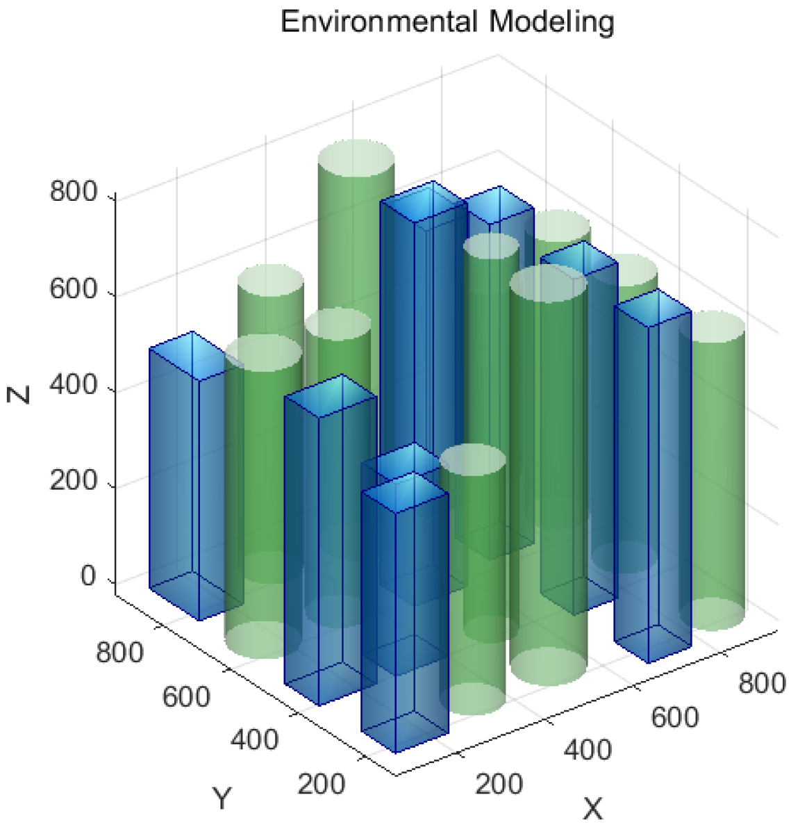
Figure 1. Environmental Modeling Diagram.
Aerospace 12 01000 g001
Figure 2. Dynamic Adaptive RRT* Algorithm Flowchart.
Aerospace 12 01000 g002
Figure 3. Dynamic adaptive sampling windows.
Aerospace 12 01000 g003
Figure 4. Schematic diagram of the dynamic sampling space.
Aerospace 12 01000 g004
Figure 5. Random 3D sampling.
Aerospace 12 01000 g005
Figure 6. Halton 3D sampling.
Aerospace 12 01000 g006
Figure 7. Bridge sampling diagram.
Aerospace 12 01000 g007
Figure 8. Side-view of truncated cone sampling.
Aerospace 12 01000 g008
Figure 9. Adaptive truncated cone sampling extension demonstration.
Aerospace 12 01000 g009
Figure 10. Comparison of PSO convergence curves after 50 iterations.
Aerospace 12 01000 g010
Figure 11. Comparison of PSO convergence curves after 100 iterations.
Aerospace 12 01000 g011
Figure 12. Comparsion of 50 iteration path.
Aerospace 12 01000 g012
Figure 13. Comparsion of 100 iteration path.
Aerospace 12 01000 g013
Figure 14. Comparison of DACS-RRT* paths.
Aerospace 12 01000 g014
Figure 15. Path graphs of different algorithms.
Aerospace 12 01000 g015aAerospace 12 01000 g015b
Figure 16. (ac) Line charts using different algorithms.
Aerospace 12 01000 g016aAerospace 12 01000 g016b
Figure 17. Bar charts of different algorithms.
Aerospace 12 01000 g017
Table 1. Specific data for different algorithms.
EnvironmentAlgorithm TypePath Length/mNode Count/nIterations/nTime/sDistance/m Turn   Angle / °
Scenario 1DACS-RRT*3136.8655.7556.750.2245.8425.96
BAI-RRT*3164.25101.70195.850.2643.1531.51
RRT*3656.541276.601551.653.3242.6630.57
BI-RRT*3425.29117.30206.350.3040.8435.89
GB-RRT*3398.16906.901354.252.5940.1927.93
RRT-Connect4133.55144.00198.650.4841.5138.58
Scenario 2DACS-RRT*3215.0589.9593.650.3146.2330.49
BAI-RRT*3332.82120.60237.550.3839.5335.57
RRT*3692.091660.302155.708.2245.9034.45
BI-RRT*3567.19191.40386.650.5644.4734.12
GB-RRT*3623.24942.951553.254.0342.3733.01
RRT-Connect4320.97239.95417.050.7142.4339.02
Scenario 3DACS-RRT*2980.1449.4050.550.2949.1523.56
BAI-RRT*3105.1585.90109.300.3846.0427.99
RRT*3515.96977.051141.554.3045.9329.04
BI-RRT*3511.71113.30166.350.4643.0034.20
GB-RRT*3406.80584.05837.803.4241.9324.94
RRT-Connect3831.9174.8088.050.3140.5828.61
Disclaimer/Publisher’s Note: The statements, opinions and data contained in all publications are solely those of the individual author(s) and contributor(s) and not of MDPI and/or the editor(s). MDPI and/or the editor(s) disclaim responsibility for any injury to people or property resulting from any ideas, methods, instructions or products referred to in the content.