A Scheduling Model for Optimizing Joint UAV-Truck Operations in Last-Mile Logistics Distribution

Abstract

This paper investigates the joint scheduling problem of unmanned aerial vehicles (UAVs) and trucks for community logistics, where UAVs act as service providers for last-mile delivery and trucks serve as mobile storage platforms for drone deployment. To address the complexity of decision variables, this paper proposes a three-stage solution scheme that divides the problem into the following: (1) UAV mission set generation via clustering, (2) truck-drone route planning, and (3) collaborative scheduling via a Mixed-Integer Linear Programming (MILP) model. The MILP model, solved exactly using Gurobi, optimizes truck movements and drone operations to minimize total delivery time, representing the core contribution. In the experimental section, to verify the correctness and effectiveness of the proposed Mixed-Integer Linear Programming (MILP) model, comparative experiments were conducted against a heuristic algorithm based on empirical intuitive decision-making. The solution results of experiments with different scales indicate that the joint scheduling model outperforms the scheduling strategies based on empirical experience across various scenario sizes. Additionally, multiple experiments conducted under different parameter settings within the same scenario successfully demonstrated that the model can stably be solved without deteriorating results when parameters change. Furthermore, this study observed that the relationship between the increase in the number of drones and the decrease in the total consumed time is not a simple linear relationship. This phenomenon is speculated to be due to the periodic patterns exhibited by the drone scheduling sequence, which align with the average duration of individual tasks.

1. Introduction

In China, most communities are independent and enclosed areas. The roads within the community are narrow, making it difficult for trucks to pass. In addition, trucks in central urban districts face strict speed limits, which further diminishes their operational efficiency. Therefore, the current logistics delivery model is that each community has its own dedicated station, where customers pick up their packages. Actually, this is not a door-to-door service. Drone delivery is a new method for achieving door-to-door service. The integration of long-distance truck transportation and short-distance drone delivery for door-to-door service in Chinese communities presents a joint scheduling problem. In this setup, the truck serves as a mobile platform for drone takeoff and landing. At each waypoint, which represents the center of gravity of the mission set, the truck can either move or wait. The center of gravity is defined as the geometric center of the customer cluster, calculated using the mean latitude and longitude of the customers. This problem involves numerous decision variables, including the truck’s route, stopping points, schedule, drone allocation, drone routes (which may differ in start and end locations), and drone scheduling. As a result, constructing and solving an overall optimization model becomes highly complex. To address this integrated challenge, three key aspects must be determined: the drone task set, the truck route, and the cooperative execution between drones and the truck. The process begins with identifying the drone task set and their execution times. Next, the truck’s route is determined. Based on the known execution and endurance times of each drone, the model allocates drones and calculates their travel times to each truck waypoint after completing tasks. This enables the system to decide whether the truck should proceed to the next station or remain at its current position. The primary objective is to minimize the total delivery time as much as possible.

Due to the fact that establishing a collaborative relationship (joint scheduling) between drones and trucks is the main optimization problem, this paper proposes a solution process pattern that divides the problem into three stages. Joint scheduling is the primary scheduling that determines the main part of optimization (the third stage). The division of distribution areas based on drone loading capacity and the planning of drone and truck routes are secondary parts of optimization (first and second stages). This article will achieve a more efficient collaborative relationship with drones by deciding whether to move or wait for trucks. This will help improve the optimization performance of the model and greatly reduce complexity. This solving method, although unable to obtain an optimized solution, can obtain quasi optimal or near optimal solutions. Because in the first stage, the division of drone delivery areas based on the number of communities, geographical location, and drone loading capacity ensures macro level optimization, in the second stage, truck and drone path planning is used to achieve micro level path optimization, and in the third stage, the adjustment of truck movement further enhances the optimization degree. In summary, it can be applied to solve practical problems in the joint transportation or distribution of trucks and drones, and has certain application value.

In the early stages of UAV involvement in logistics and distribution, UAVs are primarily viewed as auxiliary tools. For example, Murray and Chu examined the use of a single-flight UAV to assist truck delivery based on the Traveling Salesman Problem (TSP) [1]. Ferrández et al. compared the improvements in delivery time and energy consumption between collaborative and independent modes of operation for trucks and UAVs [2]. Contrary to static parking node assumptions, Marinelli et al. proposed a MILP model for dynamic drone dispatch/recovery during truck movement (not limited to fixed nodes), laying the foundation for on-the-fly coordination [3].

With the foundational model for solving the UAV-truck collaborative delivery problem established, researchers have refined scenario settings and optimized solution algorithms. Bouman et al. introduced an exact solution method for the UAV-truck traveling salesman problem (TSP-D) using dynamic programming [4]. Agatz et al. further improved Bouman’s work by developing heuristic algorithms based on local search and dynamic programming for fast path prioritization and cluster secondary [5]. Boysen et al. refined scenarios by considering the number of UAVs per truck and whether UAV takeoff and landing points are identical [6]. Ha et al. proposed a greedy randomized adaptive search procedure that delivered higher solution quality than Murray’s improved 2015 algorithm with local search [7]. Keeney and R. L. divided the problem into three subproblems and proposed a corresponding three-stage model [8]. Yurek and Ozmutlu developed an iterative, decom-position-based algorithm that assigns UAV delivery points using pre-established truck routes as the baseline [9].

As research progressed, scholars addressed the UAV-truck collaborative delivery problem based on the Vehicle Routing Problem (VRP) and began improving the efficiency of solving large-scale problems. Wang and Sheu solved the problem by incorporating constraints on UAV endurance and takeoff/landing points into the traditional VRP modeling approach [10]. To tackle the challenge of convergence to optimal solutions in large-scale problems, Sacramento et al. proposed an adaptive large neighborhood search metaheuristic algorithm [11]. Schermer et al. developed a VRP-D (Vehicle Routing Problem with Drones) model by introducing the Drone Assignment and Scheduling Problem (DASP) scheduling model [12]. Additionally, Schermer et al. proposed a heuristic algorithm based on variable neighborhood search and tabu search to enhance the efficiency of solving large-scale VRP-D problems [13].

Starting in 2020, drones increasingly became the primary agents for delivery tasks, with multi-drone delivery and single-flight visits to multiple demand points becoming key topics. Murray and Raj expanded their 2015 Flying Sidekick TSP model by increasing the number of drones collaborating with a single truck, introducing the m-FSTSP (Multiple Flying Sidekicks TSP) model [14]. Moshref-Javadi et al. proposed a model based on the Traveling Repairman Problem (TRP), allowing trucks to deploy multiple drones for delivery operations [15]. Liu et al. developed a model where drones are the main delivery agents, capable of serving multiple customer points per trip without requiring vehicles to wait at fixed points [16]. Vu et al. examined logistics problems where drones can be launched from warehouses or trucks and proposed a metaheuristic algorithm to enhance the solving speed for large-scale problems [17]. Masmoudi et al. improved the existing VRP-D model to allow drones to deliver multiple packages per trip and proposed an adaptive multi-start simulated annealing metaheuristic algorithm for solving it [18]. Zeng et al. studied the route coordination problem where drones visit multiple designated locations and periodically meet trucks for battery replacement, establishing the Nested-VRP model and solving it with a neighborhood heuristic algorithm [19]. Freitas et al. proposed an improved mixed-integer programming (MIP) formulation for solving Murray’s FSTSP model, achieving improved results in over 80% of cases [20]. Rave et al. developed a tactical planning model that combines truck-only, drone-only, and truck-drone collaborative delivery methods based on delivery demand distribution [21]. Ndiaye et al. proposed a variable neighborhood search metaheuristic algorithm for the FSTSP model, accelerating the solving speed for medium to large-scale problems [22].

For UAV-truck coordinated delivery, solution approaches can be categorized into direct optimization and dividing the problem into several subproblems for solving. The direct optimization approach typically employs a Mixed-Integer Linear Programming (MILP) model, solved via exact solvers or heuristic algorithms. This approach, rooted in TSP/VRP frameworks, faces challenges in solving efficiency as node/arc numbers increase, due to exponential growth in network complexity. In contrast, decomposition-based methods split the problem into truck routing and drone routing subproblems, linked by a scheduling model. These methods often assume static truck positions or use heuristic algorithms for scheduling, leading to suboptimal solutions and limited practical applicability. The joint scheduling model proposed herein is a MILP framework solved exactly by Gurobi, addressing the limitations of both approaches. Unlike decomposition methods, it optimizes truck-drone coordination dynamically. The three-stage solution method presented in this paper leverages the computational speed advantages of decomposition-based approaches when dealing with large-scale demand distributions, while also incorporating the benefits of integrated optimization methods for constructing and optimizing the collaborative relationship between UAVs and trucks. This method can be regarded as a balanced solution that optimizes both solution speed and the effective coordination of UAV-truck collaboration.

In summary, the community logistics solution proposed in this paper aims to minimize total delivery time, taking into account drone endurance and payload limitations, and is based on the community-distributed nature of urban logistics demand. The following assumptions are made in solving the problem:

• Trucks do not retrace their routes.
• Drones only deliver packages at customer nodes and do not pick up items.
• Trucks serve as the sole platform for cargo storage and drone launch and recovery.
• Delivery point locations and weights are known in advance, with no new delivery demands arising during the process.
• Both drone flight speed and truck travel speed are constant.
• The community airspace is fully open to drones without restrictions, allowing safe direct flights to demand points.

The paper is organized as follows: Section 2 covers model development, with Section 2.1 focusing on the generation of drone mission sets and release point locations, Section 2.2 on the truck and drone route planning and Section 2.3 on the establishment of the drone-truck collaborative model. Section 3 presents experiments and discussions, while Section 4 provides the conclusion.

2. Mathematical Programming Formulation

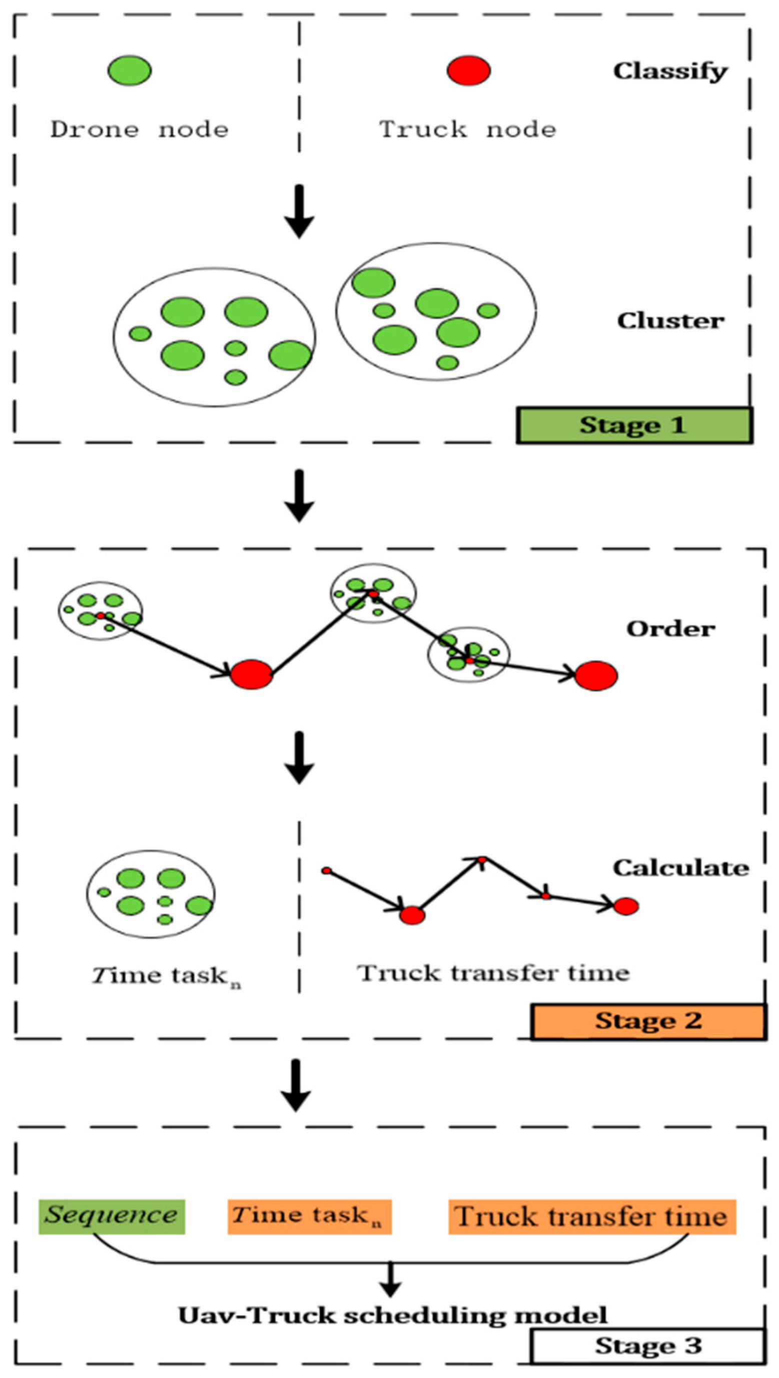
To address the terminal logistics distribution problem, this paper presents a three-stage solution scheme for UAV-truck collaborative delivery, integrating weight-based categorization, geographic clustering, and joint scheduling. The workflow is as follows:

Stage 1: Categorize items into truck-deliverable (over payload limit) and drone-deliverable (within payload limit) based on weight.

Stage 2: Cluster drone-deliverable demand points using K-means, with cluster centroids as truck release nodes, and determine truck routing via GIS-based sequencing.

Stage 3: Optimize UAV-truck coordination through a Mixed-Integer Linear Programming (MILP) model, scheduling drone missions and truck movements to minimize total delivery time. The collaborative logic across stages is visualized in Figure 1, highlighting how task duration (Stage 1–2 outputs) and operational sequences drive joint scheduling decisions (Stage 3).

The chapter details:

• Section 2.1: Task Set Generation: Clustering methodology for demand points;
• Section 2.2: Task Execution Sequencing: Truck routing and drone path planning;
• Section 2.3 (core work): Joint Scheduling Model: MILP formulation for dynamic coordination.

2.1. Generation of UAV Mission Sets and Release Point Locations

The operational limitations of UAVs are primarily constrained by their industrial load capacity and the range of their power supply. Additionally, the number of demand points that can be serviced by a single UAV release is also limited. In this paper, UAVs are firstly classified into multiple UAV delivery mission sets based on their delivery capacity limitations and the geographic distribution characteristics of the demand points. The generation of UAV mission sets is a process that can be outlined as follows: initial classification is conducted, followed by the implementation of clustering.

Initially, demand points are categorized based on the delivery weight and the drone payload limit $W_{max}$. Points exceeding the payload limit are designated as truck delivery points $d_i=0$, while those within the limit are classified as drone delivery points $d_i=1$.

Subsequently, the K-means algorithm is employed to group demand points into multiple drone delivery mission sets, with cluster centroids serving as drone release points. As a matter of intuitive experience, it can be roughly assumed that the weights of the individual tasks to be delivered close to maximum drone capacity $W_{max}$, and the initial number of clusters (mission sets) is approximated by using the upper bound of quotient of the total demanded weight ($N\ast \overline{w_i}$) divided by the UAV’s industry load limit $W_{max}$ rounded upwards, as in (1). Given that delivery points are distributed across gated communities, the final number of clusters $m\prime$ must satisfy $m\prime \ge \sum h$, where $\sum h$ is the total number of communities, ensuring each community $h$ is assigned at least one cluster point (As in (2) and (3)).

$$m=⌈{\displaystyle \frac{N\ast \overline{w_i}}{W_{max}}}⌉$$

(1)

$$\sum _k{h}_k\ge 1 \forall h$$

(2)

$$m\prime -\sum h\ge 0$$

(3)

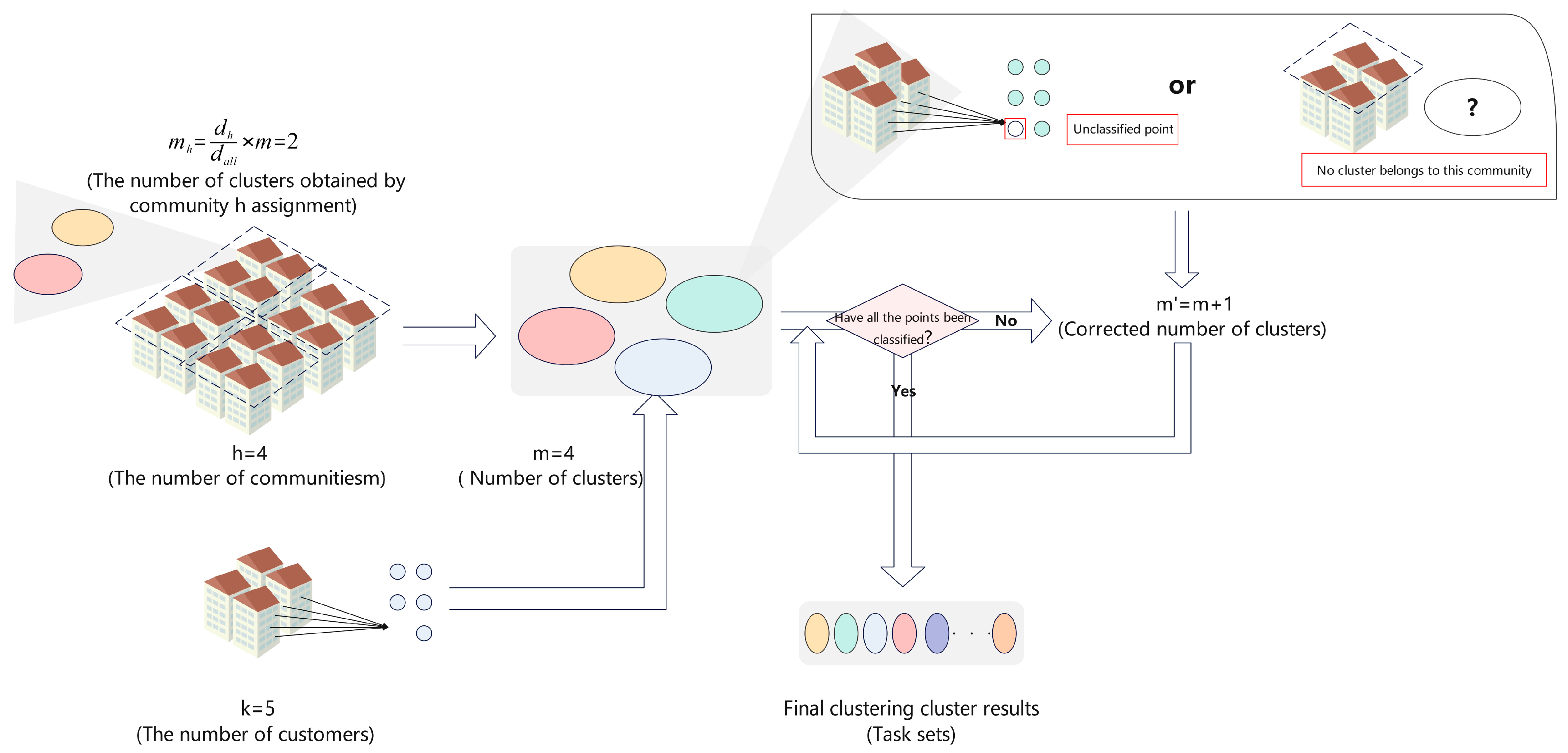
The value of $m$ is the initial number of clusters derived under the assumption of equal delivery weight at each customer node. However, in reality, weights vary across points and are distributed across gated communities. When grouping points into $m$ clusters, some points may remain non-clustered due to overweight items, exceeding flight range, or belonging to separate communities. To address this, we introduce an iterative clustering mechanism: Perform initial clustering based on pre-solved parameters. If non-clustered points exist, increment the cluster count by 1. Repeat clustering until all points are assigned, ensuring the final cluster count $m\prime$ satisfies Equation (3) ($m\prime \ge \sum h$, where $\sum h$ is the number of communities). The diagram in Figure 2 illustrates the clustering concept mentioned above.

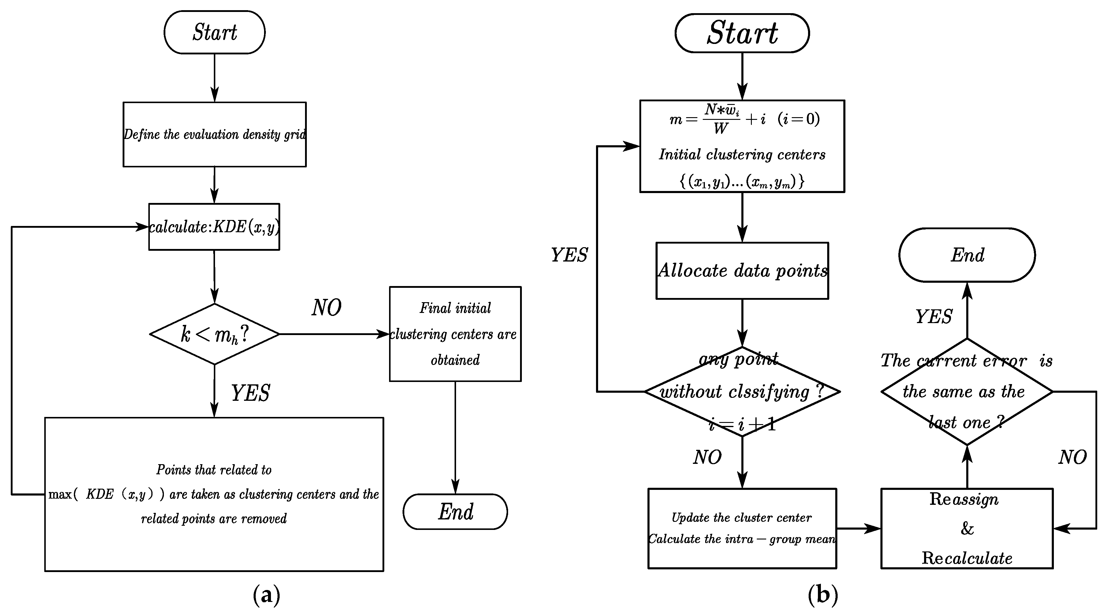
When initializing cluster centers, the number of clusters is first allocated based on the proportion of delivery points within a community relative to the total number of points $m_h$. To effectively reduce the sensitivity of clustering results to the choice of initial centers, the method of initializing K-means cluster centers using the maximum density approach based on Kernel Density Estimation (KDE) is employed. KDE is a parameter-insensitive density estimation method that is used to estimate the density of a distribution of customer points. The clustering algorithm prioritizes points with the highest KDE values (x, y) as cluster centers, selecting nodes surrounded by the densest point distributions. After the initialization of the number of clusters, the K-means algorithm is used for demand clustering.

The initialization workflow is illustrated in Figure 3a, while the full K-means process is shown in Figure 3b.

Let $m_x$ represent the x-coordinate and $m_y$ represent the y-coordinate of the task set $m$, which contains $n$ demand points (distribution points). The drone release point for task set $m$ is defined as the “center of gravity”, calculated by Equation (4).

$$(m_x,m_y)=({\displaystyle \frac{{\sum }_{i=1}^n{w}_i\ast x_i}{{\sum }_{i=1}^n{w}_i}},{\displaystyle \frac{{\sum }_{i=1}^n{w}_i\ast y_i}{{\sum }_{i=1}^n{w}_i}})$$

(4)

2.2. Path Planning for Truck Paths and Drone Paths

In this subsection, the UAV-truck delivery problem is divided into two interdependent subproblems: truck routing on ground networks and drone mission scheduling in airspace. To resolve these subproblems and their interconnections, we develop two models:

PART 1: A geographic routing model leveraging GIS APIs to compute truck travel times between pre-scheduled nodes.

PART 2: A shortest-path model using the Floyd-Warshall algorithm to optimize drone flight paths within mission sets.

These models provide foundational data (truck arrival times, drone mission durations) for the joint scheduling model in Section 2.3.

2.2.1. Calculation of Truck Node Passing Time

In this study, it is assumed that the trucks will pass through each point in a sequential manner in order to be allocated. In both academia and industry, ground path planning for trucks is a well-studied problem with established solutions. Here, truck travel times between nodes are derived using a two-step approach: Pre-sort nodes geographically (north-to-south, west-to-east ordering); Invoke a GIS mapping API (Google Maps Platform) to retrieve real-world road travel times for the pre-sorted sequence. The details are shown as follows:

Step 1: $P_D$ denotes points where trucks stop to release drones, while $P_T$ indicates points requiring truck deliveries. Since the main objective of this paper is to propose a joint scheduling model, we simplify the process in this section. Specifically, given the block-by-block nature of urban delivery, the two types of points are arranged sequentially from north to south and west to east. In this context, “Node” refers to the points that the truck sequentially passes through after the planning phase, while $P_D$ and $P_T$ represent the delivery attributes associated with these points. The northwesternmost point is designated as waypoint 1, forming a sequence of nodes for truck visitation, as shown in Figure 4.

Step 2: Invoke the route planning interface provided by the navigation map API, restricting the vehicle type to small and medium-sized trucks, to export the travel time between each truck point. Truck delivery time is cumulative to the time taken by the truck to leave point $P_T$ and travel to the next node.

Through the data processing in this subsection, the truck-related decision variables in the joint model are replaced by their arrival times at waypoints, specifically the variable $t_j$ defined in Section 2.3.

2.2.2. Solving for Drone Mission Time

The problem of solving the drone path is a classic shortest path problem in graph theory. In this paper, the problem is formulated as a graph network model. The model employs $a_{ij}$, 0–1 decision variable, where 1 indicates traversal of arc $(i,j)$ and 0 indicates no traversal. $d_{ij}$ represents the Euclidean distance between points $i$ and $j$. $S_m$ denotes the set of all points in the nth set, and $A_n$ represents the set of all arcs in the nth set.

$$\begin{array}{c}min{\displaystyle \sum _{(i,j)\in A_n}}{d}_{ij}\ast a_{ij}\\ {\displaystyle \sum _{j\in S_m}}{a}_{ij}-{\displaystyle \sum _{j\in S_m}}{a}_{ji}=\left\{\begin{array}{c}-1, i=s\\ 0, i\ne s \mathrm{and} i\ne t\\ 1, i=t\end{array}\right.\end{array}$$

(5)

In Equation (5), $s$ and $t$ denote the source node and destination node, respectively. In the context of our research problem, the truck’s path is pre-determined and fixed. As a result, the order in which the UAV services customer nodes between two consecutive truck nodes is also pre-determined, based on the spatial proximity to the truck’s movement direction. The problem we are solving for the UAV on each segment of the path is a shortest path problem through a fixed sequence of nodes. Under this problem definition, the optimal UAV path is simply the sequence of shortest paths between each pair of adjacent nodes. The Floyd algorithm is used to calculate the shortest path distances between all pairs of nodes in the graph.

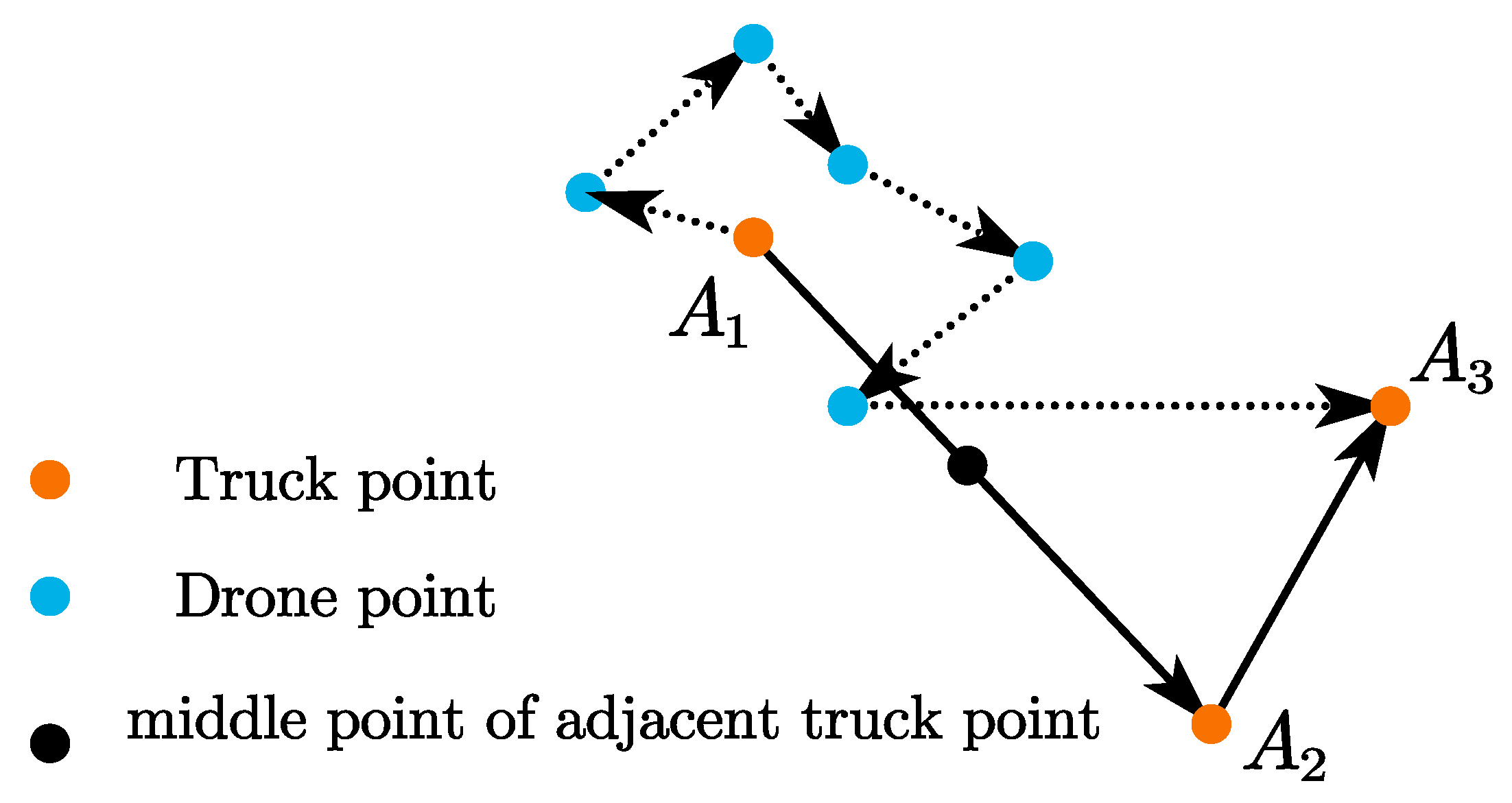
As shown in Figure 5, orange nodes represent truck routes, blue nodes denote drone flight paths, and black nodes signify midpoints. The dashed line represents the UAV’s flight path, while the solid line represents the truck’s route. Notably, the flight time from the last demand node to midpoint $t$ is omitted from the total mission time to focus on operational efficiency.

After computing the shortest total flight distance $d_m$ for task set $\mathrm{m}$, the horizontal flight time is derived as $d_m/V_d$, where $V_d$ is the drone’s constant flight speed. This time excludes vertical operations (takeoff, landing and delivery). To account for these, an average time $\mathit{\Delta }T$ (per node) is introduced. $\mathit{\Delta }T$ is a tunable parameter representing the total ground operation time, ensuring that the model considers the duration required to implement the planned interactions between the UAV and the truck. The adjusted duration is calculated as $\mathrm{n}\times \Delta \mathrm{T}$, where $n$ is the number of nodes in the task set. Thus, the total task duration ${\mathrm{T}\mathrm{i}\mathrm{m}\mathrm{e} \mathrm{t}\mathrm{a}\mathrm{s}\mathrm{k}}_{\mathrm{m}}$ for task set $\mathrm{m}$ is composed of two parts: the horizontal flight duration and the adjusted duration, as shown in Equation (6).

$${Time task}_m={\displaystyle \frac{d_m}{V_d}}+\mathrm{n}\ast ∆\mathrm{T}$$

(6)

2.2.3. Solving the Projected Recovery Nodes for Drones

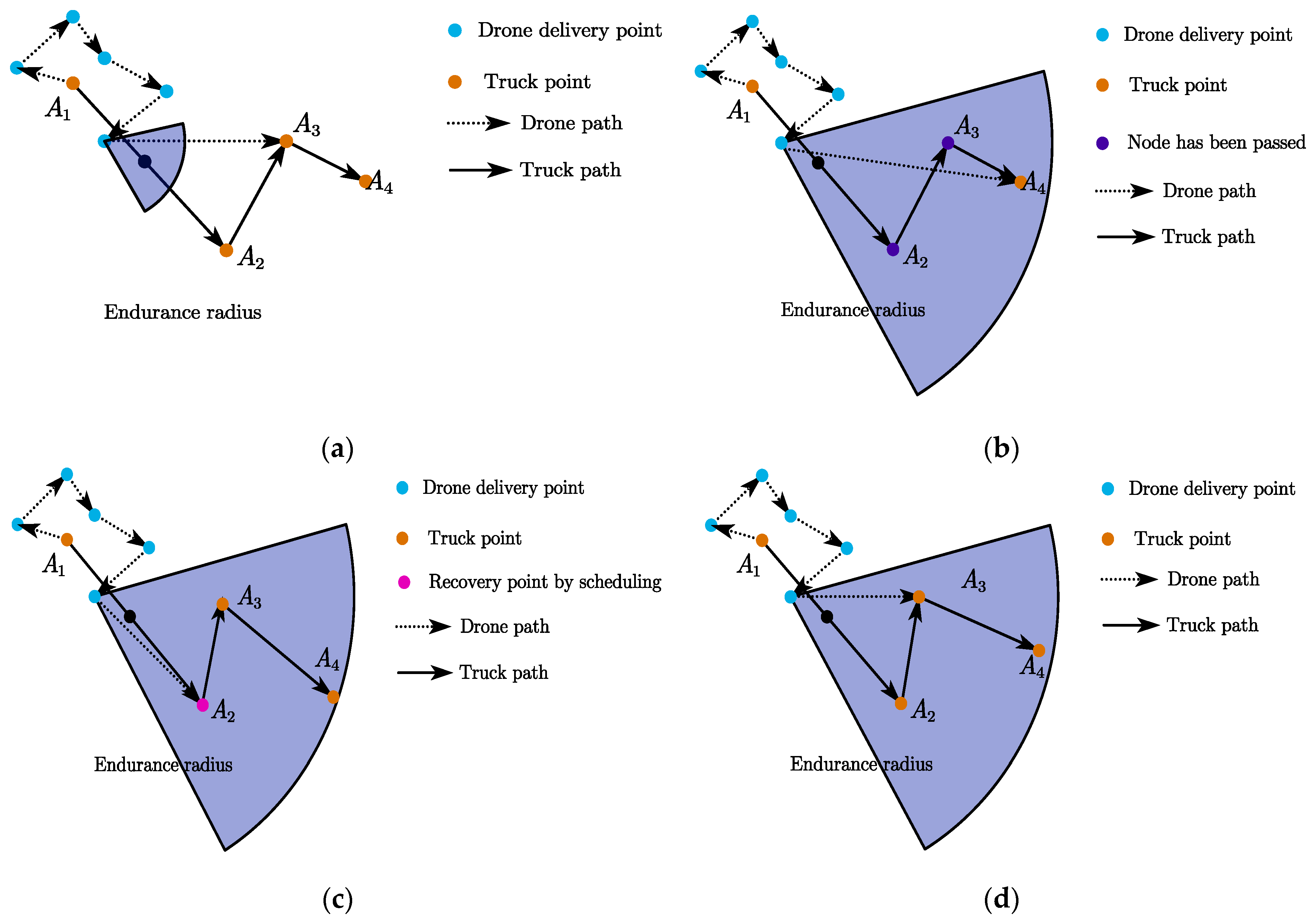
Upon task completion, drone recovery nodes are classified into two categories: the current release node or subsequent truck nodes. Given the model’s assumptions (no truck route reversal and no access to departed nodes), four recovery scenarios arise:

(a) No Subsequent Nodes Available

If no subsequent truck nodes lie within the drone’s remaining flight range, the drone recovers at the current release node. Figure 6b–d assume the drone detects subsequent nodes within its range.

(b) Truck Departed from Nearest Node

If the truck has left the nearest node by the drone’s task completion time, the drone must select an alternative recovery node where the truck is present or enroute. As shown in Figure 6b, after task completion, the truck has departed nodes $A_2$ and $A_3$, leaving only $A_4$ within range, so the drone flies to $A_4$.

(c) Scheduled Recovery Node Override

When subsequent nodes exist but scheduling dictates a specific recovery point, the drone prioritizes the assigned node over the nearest option. In Figure 6c, despite $A_3$ being closer, the drone is directed to recover at $A_2$ for operational coherence.

(d) Autonomous Recovery Selection

In the absence of scheduled points, the drone autonomously chooses the nearest accessible node or a subsequent node that avoids truck waiting. As illustrated in Figure 6d, if $A_3$ is nearest or $A_2$ requires truck waiting, the drone selects $A_3$ to minimize delays.

Based on the four potential operational scenarios outlined above, it is clear that, regardless of the type of node where the UAV performs recovery, coordination with the truck is essential. Since the sequence of node visits is predetermined and remains unchanged when new nodes are introduced, the essence of truck-UAV coordination lies in optimizing the truck’s waiting strategy and operational scheduling. This involves determining when and where to deploy and recover the UAV. To address this dynamic UAV-truck collaboration problem, a unified MILP model is proposed in Section 2.3. The MILP model introduced in this paper does not rely on specific scenario rules. Instead, it makes comprehensive decisions by simultaneously considering the truck’s route schedule, the UAV’s flight endurance, and the objective of minimizing total task time. This ensures a globally optimal solution, rather than a short-sighted, rule-based choice.

2.3. Drone-Truck Collaboration Model

The model proposed in this section treats the pre-determined truck traversal sequence as a series of task operations, enabling the joint scheduling of UAVs and trucks. This UAV-truck joint scheduling problem involves numerous parameters and variables, which can result in dimensionality and complexity issues that hinder model development and solution.

The key challenge in joint scheduling lies in coupling the UAV and truck in both time and space. To address this, key UAV parameters, such as flight capability, are converted into time metrics, facilitating system-level optimization. From a practical perspective, particularly in low-altitude logistics systems, time is often the primary optimization objective due to several driving factors. First, from an operational eco-nomic standpoint, the UAV’s limited endurance makes transport time a critical determinant of energy consumption and operational costs. Therefore, the most time-efficient path is inherently the most energy-efficient. Second, in terms of service quality, timely deliveries are a core indicator of service reliability, especially in time-sensitive scenarios like urgent deliveries or emergency logistics. This is particularly true for high-priority goods such as fresh produce or medical supplies. Furthermore, the low-altitude environment itself underscores the importance of time optimization. UAVs leverage their speed advantage by avoiding ground congestion, while the complex low-altitude airspace and safety regulations require careful path planning that minimizes uncertainty during flight. This ensures optimal system throughput and response time. Thus, prioritizing time optimization is crucial for enhancing the efficiency, reliability, and economic viability of low-altitude logistics systems.

In light of these considerations, this study establishes a scheduling model with time as the unified dimension for all parameters and decision variables. The objective is to minimize the total execution time of all tasks, which not only aligns with the goal of improving logistics efficiency but also serves as a critical lever for enhancing the economic, reliability, and overall effectiveness of low-altitude logistics systems.

2.3.1. Definitions and Model Descriptions

Sets:
$N_i$:	Set of nodes to be visited by trucks (mission sets).
${At}_{p,j}$:	Set of time cost for trucks to pass between points.
${Ad}_{p,j}$:	Set of time cost for drones to pass between points.
$D_j$:	Set of number of drones required for set $j$.
$T_j$:	The execution time of the task set $j$
$E:$	Initial endurance power value of the drone.
$D_n$:	the set of drones
Variable:
$x_{i,j}$:	Whether drone $i$ performs task $j$, 1 if yes, 0 otherwise.
$t_j$:	Truck arrival time at node $j$.
$s_j$:	When task $j$ was actually executed.
$a_{i,j}$:	Whether drone $i$ is released before node $j$, yes is 1, otherwise 0.
$e_{i,j}$:	Corrected power of drone $i$ at node $j$.
${es}_{i,j}$:	The earliest available time for drone $i$ to reach node $j$.
${r1}_{i,j}$:	Whether UAV i’s current charge can perform task $j-1$ and fly to point $j$ to be recovered, yes is 1, otherwise 0.
${r2}_{i,j}$:	Whether drone i’s current power level is sufficient to perform the whole task $j-1$, yes is 1, otherwise 0.

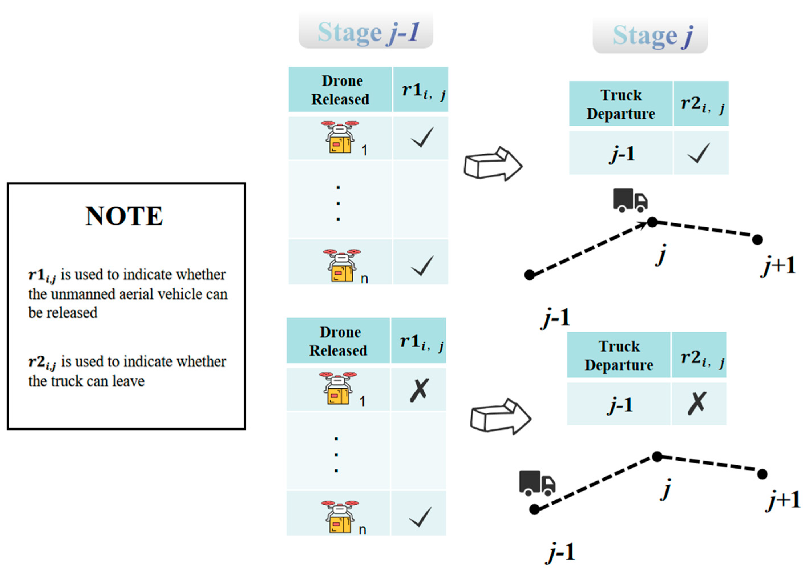
Based on the definitions of ${r1}_{i,j}$ and ${r2}_{i,j}$ in the model, the scheduling logic of the model is now explained with reference to stage $j$ and in conjunction with Figure 7. As depicted in the figure, the position of the truck at stage $j$ is determined by whether all the released drones can fly to the next node $j$ after completing their tasks. If all the released drones are able to proceed to node $j$, the truck is allowed to depart from node $j-1$ and move to node $j-1$. Otherwise, the truck must stay at node $j-1$ to wait for the return of the drones.

2.3.2. Model

$Minimize \underset{j\in N_i}{\max }{s}_j$
s.t	${\displaystyle \sum _{i=1}^k}{x}_{i,j}\ge D_j$	$\forall j\in Node$	(7)
	${\displaystyle \sum _{i=1}^k}{x}_{i,j}\le D_j$	$\forall j\in Node$	(8)
	${es}_{i,j}\ge \left({es}_{i,p}+T_p+{Ad}_{p,j}\right)\ast x_{i,p}$	$\forall i\in \mathrm{D}\mathrm{n},\mathrm{j},\mathrm{p}\in Node,\mathrm{p}<\mathrm{j}$	(9)
	${es}_{i,j}\ge t_{j-1}$	$\forall i\in \mathrm{D}\mathrm{n},\mathrm{j}\in \mathrm{N}\mathrm{o}\mathrm{d}\mathrm{e}$	(10)
	$s_j\ge {es}_{i,j}\ast x_{i,j}$	$\forall i\in \mathrm{D}\mathrm{n},\mathrm{j}\in \mathrm{N}\mathrm{o}\mathrm{d}\mathrm{e}$	(11)
	$s_j\ge t_j$	$\forall i\in \mathrm{D}\mathrm{n},\mathrm{j}\in \mathrm{N}\mathrm{o}\mathrm{d}\mathrm{e}$	(12)
	$t_j\ge s_{j-1}+{At}_j$	$\forall i\in \mathrm{D}\mathrm{n},\mathrm{j}\in \mathrm{N}\mathrm{o}\mathrm{d}\mathrm{e}$	(13)
	$t_j\ge s_{j-1}+{At}_j+T_{j-1}\ast {r1}_{i,j-1}\ast x_{i,j-1}$	$\forall i\in \mathrm{D}\mathrm{n},\mathrm{j}\in \mathrm{N}\mathrm{o}\mathrm{d}\mathrm{e}$	(14)
	$t_j\ge {es}_{i,j-1}+{Ad}_{j-1,j}-M\times (1-x_{i,j})$	$\forall i\in \mathrm{D}\mathrm{n},\mathrm{j}\in \mathrm{N}\mathrm{o}\mathrm{d}\mathrm{e}$	(15)
	$a_{i,j}\ge a_{i,j-1}$	$\forall i\in \mathrm{D}\mathrm{n},\mathrm{j}\in \mathrm{N}\mathrm{o}\mathrm{d}\mathrm{e}$	(16)
	$a_{i,j}\ge {\displaystyle \frac{1}{j}}\ast {\displaystyle \sum _{p=j+1}^n}{x}_{i,p}$	$\forall i\in \mathrm{D}\mathrm{n},\mathrm{j}\in \mathrm{N}\mathrm{o}\mathrm{d}\mathrm{e}$	(17)
	$a_{i,j}\le {\displaystyle \sum _{p=j+1}^n}{x}_{i,p}$	$\forall i\in \mathrm{D}\mathrm{n},\mathrm{j}\in \mathrm{N}\mathrm{o}\mathrm{d}\mathrm{e}$	(18)
	$e_{i,j}=E_i+{\displaystyle \sum _{p=1}^{j+1}}{(t}_p-s_{p-1})\ast (1-a_{i,p})$	$\forall i\in \mathrm{D}\mathrm{n},\mathrm{j}\in \mathrm{N}\mathrm{o}\mathrm{d}\mathrm{e}$	(19)
	$e_{i,j-1}-{es}_{i,j-1}-T_{j-1}-{Ad}_{j-1,j}+M\ast {r1}_{i,j}\ge 0$	$\forall i\in \mathrm{D}\mathrm{n},\mathrm{j}\in \mathrm{N}\mathrm{o}\mathrm{d}\mathrm{e}$	(20)
	$e_{i,j-1}-{es}_{i,j-1}-T_{j-1}-{Ad}_{j-1,j}-M\ast \left(1-{r1}_{i,j}\right)\le 0$	$\forall i\in \mathrm{D}\mathrm{n},\mathrm{j}\in \mathrm{N}\mathrm{o}\mathrm{d}\mathrm{e}$	(21)
	$e_{i,j-1}-t_{j-1}-T_{j-1}-{Ad}_{j-1,j}+M\ast {r1}_{i,j}\ge 0$	$\forall i\in \mathrm{D}\mathrm{n},\mathrm{j}\in \mathrm{N}\mathrm{o}\mathrm{d}\mathrm{e}$	(22)
	$e_{i,j-1}-t_{j-1}-T_{j-1}-{Ad}_{j-1,j}-M\ast \left(1-{r1}_{i,j}\right)\le 0$	$\forall i\in \mathrm{D}\mathrm{n},\mathrm{j}\in \mathrm{N}\mathrm{o}\mathrm{d}\mathrm{e}$	(23)
	$e_{i,j}-{es}_{i,j}-T_j+M\ast {r2}_{i,j}\ge 0$	$\forall i\in \mathrm{D}\mathrm{n},\mathrm{j}\in \mathrm{N}\mathrm{o}\mathrm{d}\mathrm{e}$	(24)
	$e_{i,j}-{es}_{i,j}-T_j-M\ast \left(1-{r2}_{i,j}\right)\le 0$	$\forall i\in \mathrm{D}\mathrm{n},\mathrm{j}\in \mathrm{N}\mathrm{o}\mathrm{d}\mathrm{e}$	(25)
	$e_{i,j}-t_j-T_j+M\ast {r2}_{i,j}\ge 0$	$\forall i\in \mathrm{D}\mathrm{n},\mathrm{j}\in \mathrm{N}\mathrm{o}\mathrm{d}\mathrm{e}$	(26)
	$e_{i,j}-t_j-T_j-M\ast \left(1-{r2}_{i,j}\right)\le 0$	$\forall i\in \mathrm{D}\mathrm{n},\mathrm{j}\in \mathrm{N}\mathrm{o}\mathrm{d}\mathrm{e}$	(27)
	$x_{i,p}\le 1-{r2}_{i,j}$	$\forall i\in \mathrm{D}\mathrm{n},\mathrm{j},\mathrm{p}\in \mathrm{N}\mathrm{o}\mathrm{d}\mathrm{e},\mathrm{p}\ge \mathrm{j}-1$	(28)
	${es}_{i,p}\ge M\ast {r2}_{i,p}$	$\forall i\in \mathrm{D}\mathrm{n},\mathrm{j},\mathrm{p}\in \mathrm{N}\mathrm{o}\mathrm{d}\mathrm{e},\mathrm{p}>\mathrm{j}$	(29)
	${es}_{i,j}\ge {es}_{i,j-1}$	$\forall i\in \mathrm{D}\mathrm{n},\mathrm{j}\in \mathrm{N}\mathrm{o}\mathrm{d}\mathrm{e}$	(30)
	${es}_{i,0}\le 0$	$\forall i\in \mathrm{D}\mathrm{n}$	(31)
	$s_0\le 0$		(32)
	${r1}_{i,0}\le 0$	$\forall i\in \mathrm{D}\mathrm{n}$	(33)
	${r2}_{i,0}\le 0$	$\forall i\in \mathrm{D}\mathrm{n}$	(34)
	$x_{i,j}, a_{i,j}, {r1}_{i,j}, {r2}_{i,j}\in \{0, 1\}$	$\forall i\in \mathrm{D}\mathrm{n},\mathrm{j}\in \mathrm{N}\mathrm{o}\mathrm{d}\mathrm{e}$	(35)
	${es}_{i,j}, s_j, t_j, e_{i,j}\ge 0$	$\forall i\in \mathrm{D}\mathrm{n},\mathrm{j}\in \mathrm{N}\mathrm{o}\mathrm{d}\mathrm{e}$	(36)

The model comprises a total of 33 constraints, explained as follows. Equations (7) and (8) differentiate between truck and drone delivery points. For truck delivery points, the value of ${\mathrm{D}\mathrm{r}\mathrm{o}\mathrm{n}\mathrm{e}\text{\_}\mathrm{n}\mathrm{e}\mathrm{e}\mathrm{d}}_j$ is set to 0, while for drone delivery points, the necessary number of drones must be released to meet demand. Equations (9) and (10) impose constraints on the earliest service time for each drone at a node. If the drone is detached from the truck platform upon arrival, its earliest available time is calculated based on its task execution status. If it remains on the truck, the time aligns with the truck’s arrival at the node. The earliest execution time for subsequent tasks $s_j$ is constrained by Equations (11) and (12) to accommodate both truck and drone conditions. Equations (13) and (15) constrain the truck’s arrival time at nodes. Ideally, the truck can leave immediately after releasing the drone, as per Equation (13). However, if the drone’s battery only suffices for the current node’s task, the truck must wait to recover the drone, as per Equation (14). Equation (15) enforces that if drone $i$ is assigned to node $j$, the truck must remain at node $j$ until the drone arrives, ensuring synchronization between truck movements and drone operations. Equations (16)–(19) correct for drone battery usage. During the truck-bound phase before release, the drone’s battery does not deplete. Thus, the first release node must be identified to adjust the battery level by adding back the amount deducted for the in-transit period. Equations (20)–(23) assess whether a drone can continue to the next adjacent node after completing a task at node $j$. If not, the current node task can be executed, but the truck must wait for recovery (as per Equation (14)). For drone $i$, task execution start time is constrained by both the drone’s earliest arrival and the truck’s earliest arrival, addressed by Equations (20) and (21) from the drone’s perspective and Equations (22) and (23) from the truck’s perspective. Equations (24)–(27) evaluate whether a drone can execute only the current node’s task. If not, Equation (28) ensures that the task is not assigned to drone $i$. Equations (29) and (30) provide logical coordination constraints: Equation (28) sets the arrival time at subsequent nodes to infinity for low-battery drones, while Equation (30) ensures that each drone’s subsequent node visit time is not earlier than the preceding node. Equations (31)–(34) assign initial values to model variables. Equations (35) and (36) define variable constraint types: $x_{i,j},{r1}_{i,j},{r2}_{i,j}$ are binary decision variables, while ${es}_{i,j},s_j$ are continuous variables. The value of big M should be a sufficiently large constant, typically set as multiples of large values such as 100 or 1000.

3. Experiment and Discussion

This chapter presents the experimental sections of the paper. Section 3.1 validates the rationality of the joint scheduling model for UAV-truck logistics delivery, which was proposed in this study. Section 3.2 conducts a multi-scale simulation experiment using the joint scheduling model with fixed truck and UAV parameters to further assess the model’s performance. Section 3.3 presents large-scale simulation experiments based on the current mainstream UAV parameter settings. Together with Section 3.2, these experiments demonstrate the robustness and generalizability of the model.

3.1. Model Plausibility Testing Experiment

3.1.1. Introduction to Experimental Methods

To comprehensively evaluate the correctness and performance of the Mixed Integer Linear Programming (MILP) model proposed in this paper, three representative heuristic algorithms were selected as benchmark methods: the Greedy Heuristic, Adaptive Large Neighborhood Search (ALNS), and Tabu Search. Below is a brief description of each algorithm:

(1)

Greedy Heuristic

The Greedy Heuristic employs a myopic decision-making mechanism, prioritizing the UAV with the earliest ready time among the currently executable tasks at each node for task allocation, without performing global optimization. The algorithm traverses the task nodes in the order of the truck’s pre-scheduled route, making local optimal decisions at each node. When multiple UAVs have the same ready time, the UAV with the greater remaining battery is preferred. If the remaining battery is the same, the UAV with the smaller index number is selected.

(2)

ALNS

ALNS is a metaheuristic algorithm that explores the solution space by adaptively selecting destruction and repair operators. The destruction operators include random removal, worst removal, and Shaw removal, each removing a proportion of tasks (e.g., q ∈ [10%, 40%]) in different ways. The repair operators include greedy insertion and Regret-2 Insertion, which are used to reinsert tasks to optimize the objective function. The algorithm uses an adaptive weight mechanism that dynamically adjusts the selection probability of operators based on the quality of the solutions produced (such as global optimal solutions or improved solutions). Additionally, it accepts new solutions probabilistically through a simulated annealing criterion, balancing exploration and exploitation.

(3)

Tabu Search

Tabu Search is a metaheuristic algorithm whose core lies in maintaining a tabu list to prohibit reverse operations recently performed, thus avoiding cyclic search and escaping local optima. The algorithm defines neighborhood operations (such as swaps and relocations) to explore the solution space. During the search process, the algorithm employs a “desperation criterion”: if a tabu move leads to a new solution that is better than the global optimum, the move is accepted as an exception.

Since both ALNS and Tabu Search are well-established frameworks for solving Mixed Integer Programming (MIP), their implementation processes are widely known. However, the Greedy Heuristic varies more depending on the specific problem being solved. Therefore, this paper provides pseudocode for the Greedy Heuristic specifically designed for this problem, as shown in Algorithm 1.

Algorithm 1 Pseudocode for the Greedy Heuristic Programming

Initialize the Duration, T-time, D-time objects.

Load data from Excel to corresponding objects (Node, Arc_d, Arc_t, Time_task, Drone_need, Drones, ED) Create a Truck object (truck_location, truck_time), including initializing internal Drone objects (drone_id, battery, max_battery, route, current_time, current_location, accumulated_energy). For each task_node in task_sequence:    If the current point is not the last point (end_node):     Calculate the required power based on task duration (Time_task[task_node]) and drone recovery time     available_drones = get_available_drones(task_node)      For each drone in available_drones:        ready_time = calculate_ready_time(drone, task_node)     Sort available_drones by:       1. ready_time (ascending)       2. If ready_time is equal: drone.battery (descending)       3. If drone.battery is equal: drone.drone_id (ascending)     If available_drones is not empty:       best_drone = available_drones[0]       move_truck_to_next_node(task_node):         truck_time += Arc_t[task_node]         truck_location = task_node       best_drone.execute_task(truck_location, truck_time, task_node, task_duration, Arc_d):         If drone.current_time < truck_time:           charge_time = truck_time − drone.current_time           potential_battery = drone.battery + charge_time           If potential_battery >= current_task_energy:             drone.battery = min(potential_battery, drone.max_battery)             drone.accumulated_energy = 0.0         drone.battery -= current_task_energy         drone.accumulated_energy = energy_consumed         drone.current_time = completion_time         drone.current_location = task_node         drone.route.append(task_node)     else:       Warning: No available drone for task_node For each drone flight:    If on the truck (first task in route):     The arrival time at the task point is the same as the truck    else:     Arrival time = drone.current_time + Arc_d[prev_task][task_node]    If released to perform a task:     The drone battery decreases over time when out from truck until it is recovered again     drone.battery -= (flight_distance + task_duration)     drone.accumulated_energy += (flight_distance + task_duration) Calculate objective function:    For each drone:     return_time = drone.get_return_time(end_node, Arc_d)    max_return_time = max(return_times) Output the total waiting time for drones on the truck and the task completion duration

The MILP model is solved exactly using Gurobi 11.0.3, while Greedy Heuristic, ALNS and Tabu Search are implemented in Python 3.9. The experimental environment is as follows: operating system, Windows 11.0 (22631.2) on a 64-bit Windows platform; CPU model, 12th Gen Intel(R) Core (TM) i9-12900H; and Gurobi Optimizer version 11.0.3 build v11.0.3rc0.

3.1.2. Preliminary Validation Through Small-Scale Experiments

To validate the MILP model, a small-scale case study is designed, comparing solutions from the two strategies (Exact Solution and Greedy Heuristic). In the $A_d$ matrix below, the first and seventh columns represent dummy nodes for initial and terminal states. Drone access restrictions to certain nodes are enforced by setting prohibitively large values $M$ for infeasible arcs. Experimental parameters for the small-scale validation are as follows.

$$A_T=\left[0, 0, 0.4, 0.4, 0.4, 0.4, 0 \right]$$

$$T_n=\left[0, 1, 2, 1, \mathrm{1,1}, 0 \right]$$

$$D_n=\left[\mathrm{0,1},\mathrm{1,1},\mathrm{1,1},0\right]$$

$$Arc\_drone=\left[\begin{array}{c} 0 \\ M\\ M\\ M\\ M\\ M\\ M\end{array}\begin{array}{c} 0\\ 0\\ M\\ M\\ M\\ M\\ M\end{array}\begin{array}{c} M\\ 0.2\\ 0\\ M\\ M\\ M\\ M\end{array}\begin{array}{c}M\\ 0.4 \\ 0.2\\ 0\\ M\\ M\\ M\end{array}\begin{array}{c}M\\ 0.7\\ 0.7\\ 0.6\\ 0\\ M\\ M\end{array}\begin{array}{c} M\\ 1.4\\ 1.2\\ 1\\ 0.4\\ 0\\ M\end{array}\begin{array}{c} M\\ M\\ M\\ M\\ M\\ 1\\ 0\end{array}\right]$$

In line with the above experimental conditions, a further breakdown of the experimental condition setup will make two assumptions about UAV power recovery. (a) the case where the default drone power can be restored instantaneously upon arrival at the platform, (b) the case where the truck is not unable to provide power restoration services for the drone. Experimental results are summarized in

Table 1. Parameter table for model test case answers.

Case	Drone	Method	Task List	Objective Function Value
Case1	1	MILP	1 → 3 → 5	3.5
		Greedy (Heuristic)	1 → 3 → 4
	2	MILP	2 → 4	3.6
		Greedy (Heuristic)	2 → 5
Case2	1	MILP	1 → 2 → 4 → 5	5.3
		Greedy (Heuristic)	1 → 2 → 4 → 5
	2	MILP	3	5.3
		Greedy (Heuristic)	3

and Figure 8. In particular, Figure 8a illustrates the results for scenario (a) discussed previously, while Figure 8b shows the results for scenario (b).

The MILP model performs better than the current optimal dynamic programming algorithm under loose experimental settings while is consistent with it under tighter settings. In the case of relaxed decision conditions (Figure 8a), the combination of locally optimal solutions is not globally optimal, and the pursuit of the earliest current mission execution will most likely sacrifice the overall time efficiency. In the case of using the MILP model to solve the case, there will be a critical node situation whose execution time cannot be further advanced, for the node’s predecessor node of other UAVs scheduling the task execution time will obtain a more relaxed decision environment. In the case of following the local optimum, the current decision is not affected by the subsequent nodes, even if a node time cannot be advanced, because the decision process is always following the current optimum, and thus each node’s decision has no posteriority. However, in the case of hard decision conditions (Figure 8b), there are not too many decision possibilities, and then the local optimal solution is also the global optimal solution.

Based on the results, it can be seen that the model in Section 2.3 can correctly solve the UAV-truck cooperative scheduling problem. Meanwhile, it can be seen that in the case where the demand is known and there is no explicit requirement on the delivery time of each demand point, the MILP scheme is better than the dynamic planning scheme of both the total solving time and the actual operational flexibility.

3.1.3. Validation Through Multi-Scale Experiments

After validating the model’s correctness through small-scale experiments, this study designed three experimental scenarios to comprehensively assess the model’s performance across different logistics distribution contexts: sparse distribution (Case 1), dense distribution (Case 2), and mixed distribution (Case 3). The sparse distribution scenario represents rural deliveries, where nodes are widely dispersed, tasks are simple, but distances are long. The dense distribution scenario, on the other hand, represents urban deliveries, where nodes are closely packed, but tasks are more complex. The mixed distribution scenario reflects suburban deliveries, incorporating both densely populated and sparsely distributed areas.

Table 2. Detailed Parameter Comparison Table for the Three Experimental Scenarios.

Case	Number of Mission Sets	Mission Time Range	Average Mission Time	Distance Range	Average Distance
1	25	[0.80, 2.50]	1.19	[0.00, 9.00]	2.94
2	25	[1.50, 3.50]	2.02	[0.00, 3.40]	1.07
3	25	[0.50, 4.00]	1.78	[0.00, 8.20]	2.55

For details of the experimental OD matrix, please refer to Supplementary Materials in the attachment.

provides a detailed comparison of the parameters for the three experimental scenarios, while

Table 3. Summary Table of Multi-Scale Validation Experiments.

Case	Method	Objective Function Value	Optimal Gap (%)	Iterations per Node	Iterations per Node	Time of Optimal Solution Discovery	Solver Runtime of the Optimizer (s)
1	MILP	18.40	0.00	1 (B&B Node Count)	-	-	0.11
	Greedy	29.90	62.50	25	-	-	<0.01
	ALNS	29.20	60.87	531	54	0.03 s (7.0%)	1.21
	Tabu Search	29.10	58.15	379	76	0.20 s (1.0%)	19.78
2	MILP	25.50	0.00	1,698,187 (B&B)	-	-	38.61
	Greedy	31.05	21.76	25	-	--	<0.01
	ALNS	30.40	19.22	500	51	0.00 s (0.0%)	0.38
	Tabu Search	30.25	18.63	302	61	0.21 s (1.3%)	15.26
3	MILP	22.80	0.00	187,451 (B&B)	-	-	7.77
	Greedy	34.45	51.10	25	-	-	<0.01
	ALNS	34.25	49.12	803	81	0.53 s (40.3%)	0.41
	Tabu Search	33.80	48.25	303	61	0.45 s (1.2%)	15.69

summarizes the experimental conditions. Finally,

Table 4. Detailed Statistical Information Table for Gurobi Solver.

Case	Objective Function Value	MIP Gap	B&B Node Count	Gap with Optimal Heuristic Solution Value
1	18.40	0.54%	1	58.15%
2	25.50	1.96%	1,698,187	18.63%
3	22.80	1.32%	187,451	48.25%

presents detailed statistical information for the Gurobi solver.

In terms of solution quality, Gurobi achieves the optimal solution in all three scenarios (MIP Gap < 2%). The objective function values are reduced by 36.7% in the sparse scenario, 18.6% in the dense scenario, and 48.2% in the mixed scenario, compared to the optimal heuristic solutions. This confirms the effectiveness of the MILP model, demonstrating that it is well-constructed and exhibits good numerical stability. Among the heuristic algorithms, the Greedy algorithm is the fastest (<0.01 s) but provides the poorest solution quality, with gaps ranging from 21.76% to 62.50%. ALNS performs best in the dense scenario, with a gap of 19.22%, but its gap in the mixed scenario increases to 49.12%. Tabu Search offers slightly better overall performance, but in the sparse scenario, the gap remains as high as 58.15%. Notably, the differences between algorithms are generally smaller in the dense scenario, as the limited feasible domain reduces the variation in scheduling strategies.

In terms of computational efficiency, Gurobi’s solution times are 0.11 s, 74.71 s, and 8.92 s for the sparse, dense, and mixed scenarios, respectively, with corresponding branch-and-bound node counts of 1, 1,698,187, and 187,451. The significant increase in computational complexity in the dense scenario is due to the small inter-node distances and long task times, which lead to a large number of feasible UAV scheduling solutions, thereby expanding the size of the branch-and-bound tree. Among the metaheuristic algorithms, ALNS solves quickly (0.40–1.32 s), with an average iteration time of 0.76–1.64 milliseconds. In contrast, Tabu Search requires significantly more time (16.66–37.55 s), with each iteration taking 51.07–123.92 milliseconds due to the overhead from neighborhood evaluation and tabu list maintenance.

In summary, Section 3.1.2 and Section 3.1.3 systematically validate the model’s correctness and performance through small- and medium-scale experiments. For correctness, the consistency between the manually derived results and the model’s solutions in small-scale cases confirms its accuracy. Regarding effectiveness, the medium-scale experiments show that the exact method significantly outperforms various heuristic algorithms in terms of solution quality. In terms of robustness, the model consistently finds optimal solutions across the three distinct scenarios. Finally, for scalability, the model can solve medium-scale problems (25 task nodes and 2 UAV sets) to optimality within 75 s, establishing a foundation for subsequent application-based experiments.

3.2. Multi-Scale Application Experiments

This chapter designs four experiment scales: small, medium, medium-large, and large. In the community terminal logistics scenario, the truck speed is set to 30 km/h. UAV parameters reference the Fengyi Fangzhou 150 model, with a maximum payload of 50 kg and cruising speed of 72 km/h. Specific experimental parameters are listed in

Table 5. Parameter table for four scales of experimental base setup.

Size	Total Task Points	Total Number of Mission Sets	UAV Parameters		Truck
small	10~100	10	velocity	72 km/h	30 km/h
medium	15~150	15
medium large	20~200	20	load capacity	50 kg	/
Large	25~250	25

For details of the experimental OD matrix, please refer to Supplementary Materials in the attachment.

, and results from 27 experimental runs are visualized in Figure 9.

In Figure 9, the green dashed line denotes the drone saturation threshold, separating results into two regions:

Below the line: Regions where drone count $\mathrm{k}<\mathrm{k}*$, and each additional drone significantly reduces the final task’s earliest completion time (${\mathrm{T}}_{\mathrm{end}}$).

Above the line: Regions where $\mathrm{k}\ge \mathrm{k}*$, indicating diminishing returns–additional drones no longer substantially decrease total task duration.

Analysis shows that as $\mathrm{k}$ increases beyond $\mathrm{k}*$, the marginal improvement in ${\mathrm{T}}_{\mathrm{end}}$ progressively declines, approaching less than 1% relative reduction.

As shown in

Table 6. Final Task Point Execution Time Advance Improvement Scale.

Total Number of Mission Sets	Number of Drones
	$∆\mathit{t}\left(\mathit{f}\mathit{i}\mathit{n}\mathit{a}\mathit{l}\right)<0.2\mathit{h}$	$∆\mathit{t}\left(\mathit{f}\mathit{i}\mathit{n}\mathit{a}\mathit{l}\right)<0.1\mathit{h}$
10	5	5
15	6	7
20	7	7
25	7	8

, the number of UAVs required to achieve $∆t\left(final\right)<0.1h$ remains fixed at around seven groups, even as the problem size increases. While this plateau reflects the law of diminishing returns in multi-UAV deployment, it also stems from how the experimental parameters mirror community-logistics characteristics—namely, nearly uniform task execution times and only slight variation in travel times. These conditions induce a cyclic structure across any seven adjacent nodes, enforcing a fixed service sequence for each UAV and thereby capping overall efficiency gains despite significant problem-scale growth.

3.3. Multi-Instance Test Experiment

In Section 3.2, the Fengyi Fangzhou 150 drone was used as a baseline case for preliminary experiments in a simulated urban community area of Nanjing. To further validate the joint scheduling model’s generalizability, large-scale experiments were conducted with one truck and two drones across 250 customer points distributed in a metropolitan logistics zone [5 km × 5 km], using three mainstream logistics drones: China Post’s Fangzhou 150, JD.com’s JDX-20 and SF Express’s PW.Orca.

Table 7. Final Task Point Execution Time Advance Improvement Scale.

Drone Models	Loading Capacity	Velocity	Total Number of Mission Sets
Fangzhou 150	50 kg	72 km/h	6
PW.Orca	15 kg	130 km/h	18
JDX-20	10 kg	98 km/h	25

Notice: For details of the experimental OD matrix, please refer to Supplementary Materials in the attachment.

lists the payload, speed, and endurance parameters for each drone. Figure 10 depicts cross-drone task allocation and truck routing across the geographic zone, with Figure 10a–c showing detailed spatial distributions for the Fangzhou 150, PW.Orca, and JDX-20, respectively. Quantitative outcomes are summarized in

Table 8. Final Task Point Execution Time Advance Improvement Scale.

Drone Models	Drone	Task List	Objective Function Value	Solver Runtime of the Optimizer
Fangzhou 150	1	2 → 4 → 6	6.17 h	0.10 s
	2	1 → 3 → 5
PW.Orca	1	1 → 3 → 5 → 6 → 8 → 9 → 11 → 13 → 16 → 18	6.6 h	0.46 s
	2	2 → 4 → 7 → 10 → 12 → 14 → 15 → 17
JDX-20	1	1 → 4 → 7 → 8 → 10 → 13 → 15 → 17 → 19 → 21 → 23 → 25	6.7694 h	0.85 s
	2	2 → 3 → 5 → 6 → 9 → 11 → 12 → 14 → 16 → 18 → 20 → 22 → 24

.

Drone parameter variations (payload, flight speed) directly influence task set partitioning and truck routing decisions, altering the joint scheduling model’s input parameters. Experimental results highlight the model’s robustness: it maintains solution feasibility across diverse parameter configurations, with adjustments primarily reflecting numerical changes in outputs rather than degradation in solution quality.

4. Conclusions

This paper addresses the drone-truck collaborative scheduling problem in community-based demand scenarios. Existing methodologies predominantly build on two classic optimization frameworks: the Vehicle Routing Problem with Drones (VRPD) and Traveling Salesman Problem (TSP), often transformed into VRP with Drone Delivery (VRPDD) or multi-Drone TSP (TSP-mD) models that enforce constraints via graph-theoretic edge/node traversal rules. However, these approaches suffer from combinatorial explosion in complex networks and scalability limitations for large-scale problems. Since the VRPD problem was initially considered a special case of vehicle scheduling, this paper focuses on scheduling optimization to solve the truck–drone collaborative delivery problem. A three-stage optimization model for community terminal logistics is proposed, featuring adaptability to both dense urban and sparse suburban operation point distributions. Comparative experiments validate the model’s feasibility, demonstrating superior solution quality over heuristic baselines and highlighting its practical utility in multi-agent scheduling contexts.

Notably, the current model incorporates several simplifying assumptions to maintain focus on the core scheduling mechanism, including predetermined truck routes without backtracking, simplified platform service times and capacity, constant speed and deterministic operating conditions. These choices, while enabling a tractable and insightful analysis of cooperative logistics, highlight specific limitations in real-world applicability, such as the exclusion of route reversals and concurrent operational constraints.

Meanwhile, although this research establishes a robust scheduling framework, real-world community logistics entail granular constraints such as zone-specific delivery agreements and drone airspace authorization protocols. Future work will focus on integrating these operational nuances into an enhanced model and optimizing solution efficiency for large-scale implementations. In addition, we plan to extend the current deterministic framework to handle stochastic elements commonly encountered in dynamic environments, as illustrated in Figure 11. Potential extensions will address:

• Demand uncertainty: via robust optimization or scenario-based approaches;
• Weather impacts: using chance constraints or real-time weather API integration;
• Drone battery uncertainty: through stochastic battery consumption models;
• Travel time variability: by incorporating buffer times or contingency strategies;
• Actual deployment differences: by establishing a more refined service time model and deck capacity constraints.