Reduced-Order Modeling and Active Subspace to Support Shape Optimization of Centrifugal Pumps

Abstract

This study presents a reduced-order modeling framework for the shape optimization of a centrifugal pump. A database of CFD solutions is generated using Latin Hypercube Sampling over five design parameters to construct a reduced-order model based on proper orthogonal decomposition with radial basis function interpolation. The model predicts the flow field at the impeller–diffuser interface and pump outlet, enabling the estimation of impeller torque and total pressure rise. The active subspaces method is applied to reduce the dimensionality of the input space from five to four modified parameters. The sensitivity of the ROM is assessed with respect to further dimensionality reductions in the parameter space, POD mode truncation, and adaptive sampling. The model is then used to perform pump shape optimization via a quasi-Newton method, identifying the combination of the parameters that minimizes the impeller torque while satisfying a constraint on the head. The optimal result is validated through CFD analysis and compared against the Pareto front generated by a genetic algorithm. The work highlights the potential of model-order reduction techniques in centrifugal pump optimization.

1. Introduction

Centrifugal pumps are fluid machines employed in a broad spectrum of different applications, ranging from industrial processes to aerospace systems. They play a pivotal role in emerging technologies, such as hydrogen-powered aircraft fuel systems [1]. In this field, their development is considered an enabling technology due to the lack of knowledge related to cryogenic pumps in aeronautics [2]. In fact, although a large amount of different ${\mathrm{LH}}_2$ pumps have been fabricated in the rocket industry [3], a pump suitable for an aircraft requires rather different features, including lower flow rates and much longer continuous reliable operation and lifetime [2]. Moreover, the absence of widely recognized standards specific to liquid hydrogen in aviation further complicates the development process. Current airworthiness regulations do not account for hydrogen as fuel [4], and the only existing guidelines in the aerospace sector pertain to the space industry—such as NASA documentation on ${\mathrm{LH}}_2$ safety [5] and pump design criteria [6,7]. Consequently, optimizing centrifugal pump performance has become of utmost importance in current aerospace engineering research.

However, this task is far from straightforward: the design process of a centrifugal pump is characterized by competing objectives that must be carefully balanced. Starting from operational requirements (i.e., delivering a certain flow rate at a specific pressure), the choice of the pump architecture is constrained by both mechanical and hydrodynamic considerations [6]. For example, higher rotational speeds are desirable because they lead to a smaller size of the pump. Moreover, for most centrifugal designs—typically those operating within a moderate range of specific speeds, before transitioning to mixed or axial flow configurations—increasing the rotational speed (with the flow rate and head per stage being fixed) also increases the hydraulic efficiency of the pump [7], that is, the ratio of hydraulic power to shaft power. In contrast, rotational speed is limited by several factors, including shaft critical speed, bearing operating life requirements, maximum allowable tip speeds, and suction performance [6].

Also, reducing the axial length is a key objective to achieve a more lightweight and cost-effective machine. However, sufficient space must be preserved within the flow path to allow the fluid to change direction efficiently [8].

Classical design guidelines based on empirical correlations can be applied for preliminary sizing [8,9], yielding an initial configuration that may serve as a reference for further refinements. While such methods provide a practical starting point, a variety of advanced optimization techniques have been developed to improve pump performance, including genetic algorithms applied to parallel pump systems [10], particle swarm optimization approaches [11], and shape optimization with the artificial bee colony algorithm [12].

To effectively apply such optimization strategies and compare alternative design solutions, it is essential to generate high-fidelity data. Such data can be obtained either through dedicated experimental campaigns or via computational fluid dynamics (CFD) simulations. While CFD offers a cost-effective and time-saving alternative to physical testing, it nonetheless remains computationally intensive, even when leveraging domain periodicity—where applicable—to reduce the computational effort. To address this limitation, one possible solution is the use of surrogate models trained on a limited set of expensive CFD simulations. Examples include artificial neural networks (as in Refs. [10,11] and in Ref. [13], in conjunction with other surrogate models) and reduced-order models (ROMs); among the various model reduction techniques, one of the most widely employed is proper orthogonal decomposition (POD) [14].

The POD approach provides an optimal (in the least-square sense) orthonormal basis for a given set of experimental data [14]; in other words, it enables the identification of the most significant features within a dataset derived from experiments or simulations [15]. For this reason, proper orthogonal decomposition found its first applications in fluid dynamics, more specifically in the field of turbulence, as an attempt to uncover deterministic structures hidden within the apparently random behavior of the flow [16]. The pioneering work by Lumley [17] laid the foundation for a broad research area that had inspired numerous studies over the years [18,19], including those of Sirovich [20]. In addition, POD has also been employed in conjunction with high-fidelity models through domain-decomposition strategies in incompressible flow simulations, as in Ref. [21]. Beyond fluid mechanics, proper orthogonal decomposition has found widespread application in diverse fields such as pattern recognition [22], control design [23], and structural damage identification [24]. More recently, it has been applied to the design and optimization of turbomachinery [25,26].

In the present paper, a reduced-order model based on proper orthogonal decomposition is employed to find the optimal combination of some of the design parameters of a hydrogen centrifugal pump for aeronautical applications. A design of experiments (DoE) based on Latin hypercube sampling (LHS) is conducted on five different geometric parameters (Section 2): by running a CFD analysis for each geometry in the database, the high-fidelity data for the reduced-order model are created (Section 3). Prior to building the ROM across all five input parameters, the dimensionality of the problem is assessed and potentially reduced using the active subspaces technique (Section 4). Eventually, the error on ROM prediction is quantified (Section 5), as well as the impact of further dimensionality reductions in the input space, POD mode truncation, and database refinement (Section 6). Finally, the model is iteratively queried by a gradient-based algorithm to evaluate torque and head at each design configuration, enabling the identification of the optimal parameter set that minimizes impeller torque subject to a minimum head requirement (Section 7).

Other recent studies on the optimization of centrifugal pumps for aerospace applications rely on models that estimate global performance metrics—such as head or efficiency—using response surface methods [27,28], analytical formulations [29], or artificial neural networks [30]. In contrast, the proposed ROM-based approach enables fast and accurate prediction of head and torque by reconstructing the full flow field in critical regions of the domain, such as the diffuser outlet and the impeller–diffuser interface, thus providing deeper physical insight into the optimal geometry selection. Moreover, the identification of an active subspace within the input parameter space further enhances the computational efficiency of the model compared with high-fidelity simulations.

2. Problem Overview

The high pressure ${\mathrm{LH}}_2$ pump for aeronautical applications proposed by Brewer [1] is selected as the case study for the following optimization process. The machine is a two-stage centrifugal pump delivering a flow of 386 L/min, with a head rise of about 7510 m rotating at 50,000 rpm. The rotational speed at design point and the number of stages are kept fixed, because they result from complex mechanical and fluid dynamic trade-offs, as discussed in Section 1. Additionally, a maximum radial envelope for the impeller–diffuser assembly is also defined, which will determine a constraint for the extension of the computational domain for the high-fidelity simulations. Based on the technical drawings provided by Brewer, this maximum envelope is here set to 140 mm.

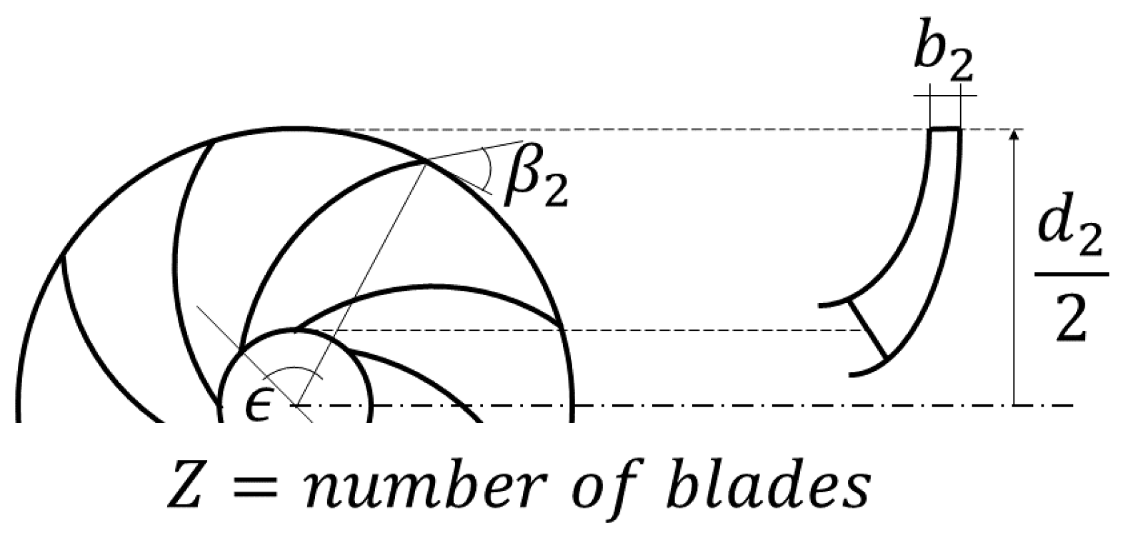
An initial database comprising 100 distinct geometries is generated. Each configuration includes an impeller and a radial diffuser with an outer diameter of 140 mm, while varying in the following five parameters: impeller diameter $d_2$, impeller blade exit width $b_2$, impeller exit blade angle ${\beta }_2$, impeller blade wrap angle $ϵ$, and number of impeller blades Z. These parameters are among the most relevant geometric quantities that define the shape of a centrifugal pump impeller, as discussed in Ref. [9]. All these quantities are shown in Figure 1:

The goal of the optimization process is to identify the combination of these parameters that minimizes the impeller torque—thus minimizing the shaft power, given the fixed design rotational speed—while providing at least the same head rise in Brewer’s pump. In this preliminary design, the diffuser is assumed to be vaneless, which enables the exploitation of the periodicity of the impeller to reduce the computational domain and, consequently, the cost of the CFD simulations. Conversely, a vaned diffuser typically requires a different periodicity than that of the impeller blades to avoid pressure pulsations [9], thereby preventing any domain reduction if unsteady rotor–stator interactions need to be accurately captured. Finally, the assumption of a vaneless diffuser does not limit the optimization process since all the five selected parameters are related solely to the impeller geometry; the presence of the diffuser allows taking into account the effect on head of total pressure losses downstream of the impeller. These losses vary under off-design conditions—which are beyond the scope of the present on-design optimization—but the vaneless diffuser has the advantage of being insensitive to variations in flow incidence [9], which typically occur when the flow rate deviates from its nominal value.

To determine the range of variation in all the selected parameters, i.e., the parameter space, the classical design guidelines mentioned in Section 1 can be used as a starting point. These guidelines are based on empirical correlations, typically expressed as functions of the specific speed of the pump. This parameter, in its adimensional form, is defined as

$${\Omega }_S={\displaystyle \frac{\omega ·\sqrt{Q}}{{(g·H_{stage})}^{3/4}}}$$

(1)

where $\omega$ is the rotational speed of the pump, Q is the volumetric flow rate, g is the gravitational acceleration, and $H_{stage}$ is the head per stage. The latter quantity is related to the stage total pressure rise $\Delta P_{T,stage}$ (i.e., the difference between total pressure at the outlet of the stage and that at the inlet) as follows:

$$H_{stage}={\displaystyle \frac{\Delta P_{T,stage}}{\rho ·g}}$$

(2)

where $\rho$ is the density of the fluid. Karassik [8] provides the following formula for the “typical” pressure coefficient as a function of ${\Omega }_S$:

$$\psi ={\displaystyle \frac{0.4}{{\Omega }_S^{1/4}}}$$

(3)

The pressure coefficient is defined as [8]

$$\psi ={\displaystyle \frac{g·H_{stage}}{{\omega }^2·{\displaystyle \frac{d_2^2}{4}}}}$$

(4)

For the case under study, ${\Omega }_S=0.158$ and $\psi =0.635$; by combining Equations (3) and (4), the resulting impeller diameter is $d_2=92$ mm. Consequently, the value range for the optimization of $d_2$ is chosen as $\pm 5\%$ of the value obtained by applying the classical design guidelines provided by Karassik [8]. An analogous relation to Equation (3) is also provided for the flow coefficient, namely [8]

$$\varphi =0.1715·\sqrt{{\Omega }_S}$$

(5)

The flow coefficient is defined as

$$\varphi ={\displaystyle \frac{c_{m2}}{U_2}}={\displaystyle \frac{c_{m2}}{\omega ·{\displaystyle \frac{d_2}{2}}}}$$

(6)

where $U_2$ is the blade tangential velocity at the impeller outlet and $c_{m2}$ is the flow meridional velocity at the same flow station; the latter quantity can be related to the blade exit width $b_2$ through the following expression:

$$c_{m2}={\displaystyle \frac{Q}{\pi ·d_2·b_2·\lambda }}$$

(7)

where $\lambda$ is a dimensionless blockage coefficient that accounts for the effect of the thickness of the blades and the presence of boundary layers on the surfaces of the flow passages [8]. By combining Equations (1) and (4)–(7), it is possible to write [8]

$${\displaystyle \frac{b_2}{d_2}}=0.5·{\displaystyle \frac{{({\Omega }_S·\psi )}^{3/2}}{0.343·\pi ·\lambda }}$$

(8)

For the case under study, by considering $\lambda =0.85$ as a typical value [8], the initial guess for the exit blade width is about $b_2=1.6$ mm. The range for the optimization of $b_2$ is selected by varying the value of $b_2/d_2$ obtained from Equation (8) by $\pm 10\%$.

Finally, for the remaining three parameters, the investigated intervals are chosen based on typical values reported in the literature. The outlet angle ${\beta }_2$ is varied between 25° and 40°, within the range observed in actual pump designs listed in Ref. [6]. The wrap angle is explored within 120° and 150°, in agreement with the values recommended in Ref. [9]. Lastly, for the number of blades—being the only discrete parameter—only two values, five and six, are considered, as they are among the most commonly employed in centrifugal pumps according to Guelich [9]. The complete range of variation in the selected design parameters is summarized in

Table 1. Range of variation in the selected design parameters for subsequent optimization.

Design Variables	${\mathit{d}}_2$ [mm]	${\mathit{b}}_2$ [mm]	${\mathit{\beta }}_2$ [°]	$\mathit{ϵ}$ [°]	Z
Upper bound	96.61	1.84	40	150	6
Lower bound	87.41	1.36	25	120	5

.

As anticipated in Section 1, the selected parameter space is then sampled by means of Latin hypercube sampling (LHS), which is an alternative technique to random sampling that simultaneously stratifies the parameter space on all input dimensions [31]. That is, the range of variation in each input variable is divided into a specified number of smaller intervals of equal probability, and the algorithm ensures that each interval is represented by a point in the resulting database [32]. For the discrete parameter—the number of blades, which could be either five or six—LHS was also applied initially, and the resulting continuous values were subsequently mapped to discrete numbers using a thresholding approach. A first database of 100 different points is generated, each consisting of a different combination of the design parameters; such a database is graphically displayed in Figure 2.

The resulting sample points are employed to perform a design of experiments (DoE), generating high-fidelity data through computational fluid dynamics (CFD) simulations; this topic is discussed in Section 3.

3. High-Fidelity Simulations

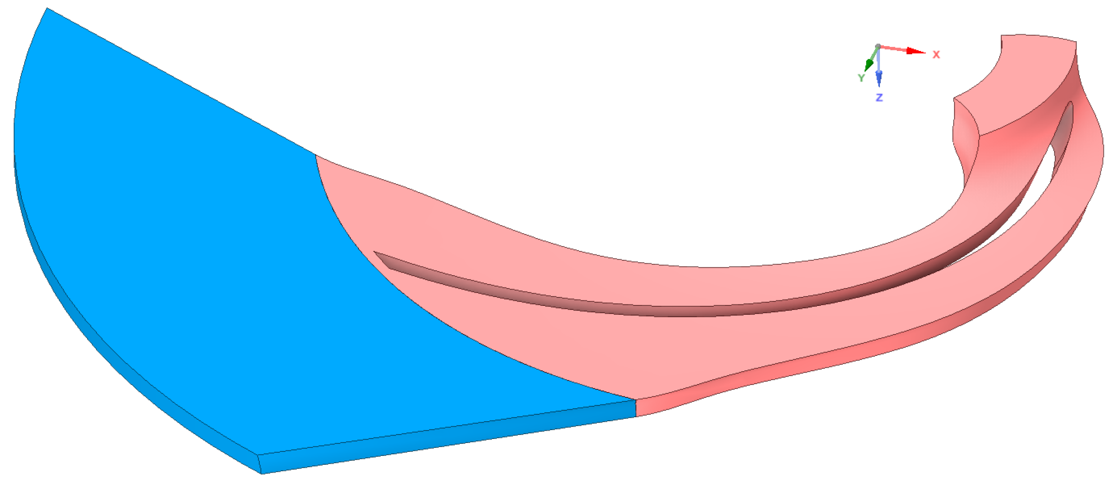
As outlined in Section 2, for each point in the database, the calculation domain consists of a periodic segment of an impeller and a vaneless diffuser. All the geometries are generated by means of the commercial software CFturbo (version 2022 R1.0): an example is displayed in Figure 3. The simulations are performed using Ansys Fluent under steady-state conditions employing the frozen rotor approach. While the impeller–diffuser interaction is inherently unsteady, steady-state simulations offer substantial computational savings and are widely employed in centrifugal pump optimization studies involving impeller–diffuser or impeller–volute configurations [33,34]. The frozen rotor method computes the flow field at a fixed relative angular position between rotating and stationary domains [9], which can introduce inaccuracies when strong rotor–stator interactions are present—particularly in the case of vaned diffusers. However, in the present study, the diffuser is vaneless, and the resulting geometric symmetry makes the relative position between impeller and diffuser not significant. For all these reasons, the steady-state approach appears appropriate for the intended preliminary optimization. The Reynolds-Averaged Navier–Stokes (RANS) equations are solved with the Spalart–Allmaras turbulence model. Boundary conditions include total pressure at the inlet and mass flow rate at the outlet, with values consistent with those reported by Brewer [1]; the fluid is treated as incompressible. This approximation is justified by the preliminary nature of the optimization, which requires a compromise between accuracy and computational efficiency for rapid design space exploration. However, the subsequent ROM framework is fully adaptable to more refined CFD models that account for density and temperature variations in the cryogenic fluid, as it relies solely on the output data extracted from high-fidelity simulations. Finally, a pressure-based solver with a coupled scheme is selected, along with second-order spatial discretization.

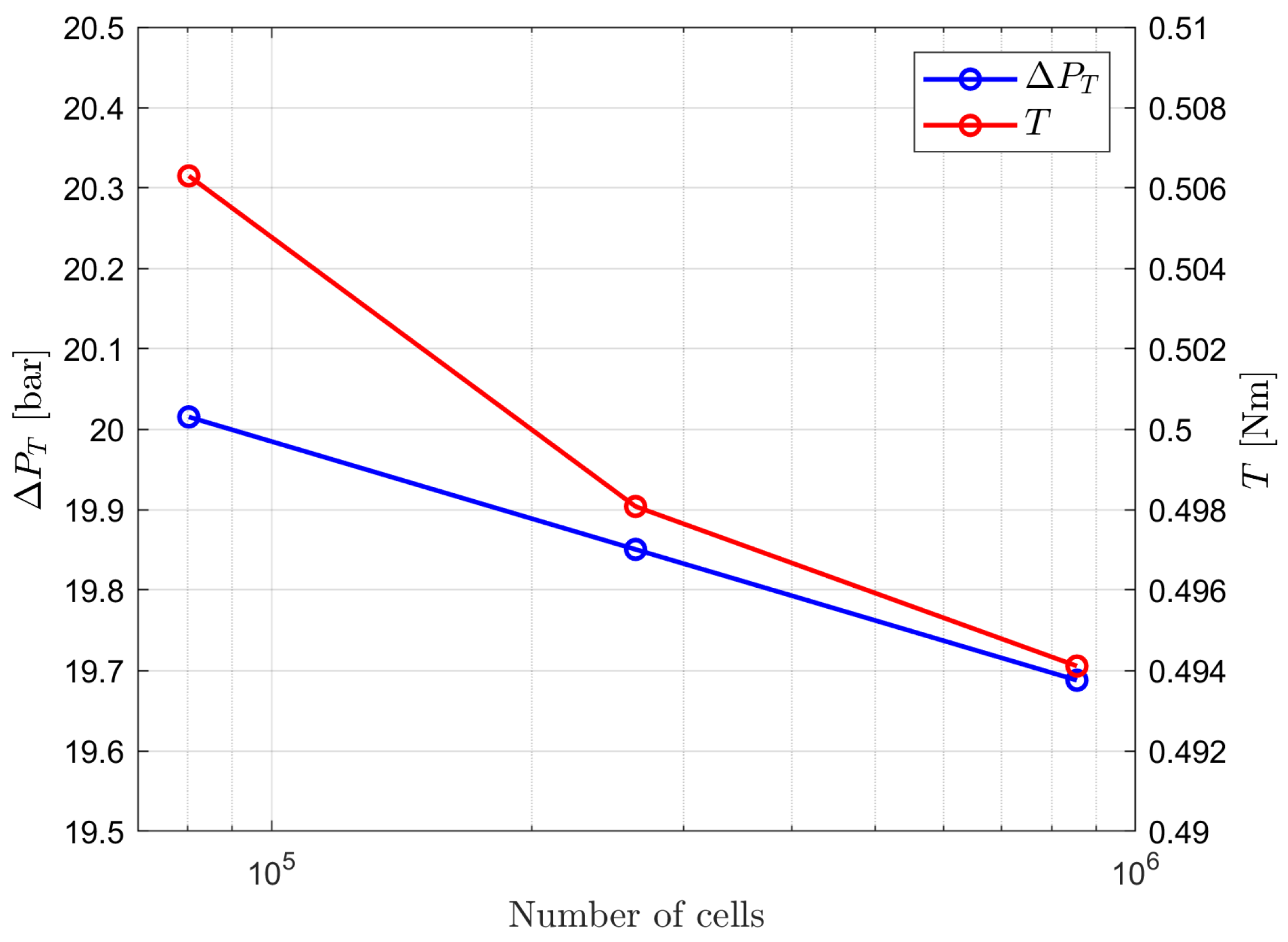
A mesh sensitivity analysis is conducted to determine an appropriate grid resolution for the CFD calculations. The test case is selected as the point in the database closest to the center of the parameter space, which is considered representative of all the geometries under study. Three different mesh sizes are compared by evaluating the variation in total pressure rise $\Delta P_T$ and impeller torque T (calculated over the single periodic sector), as shown in Figure 4.

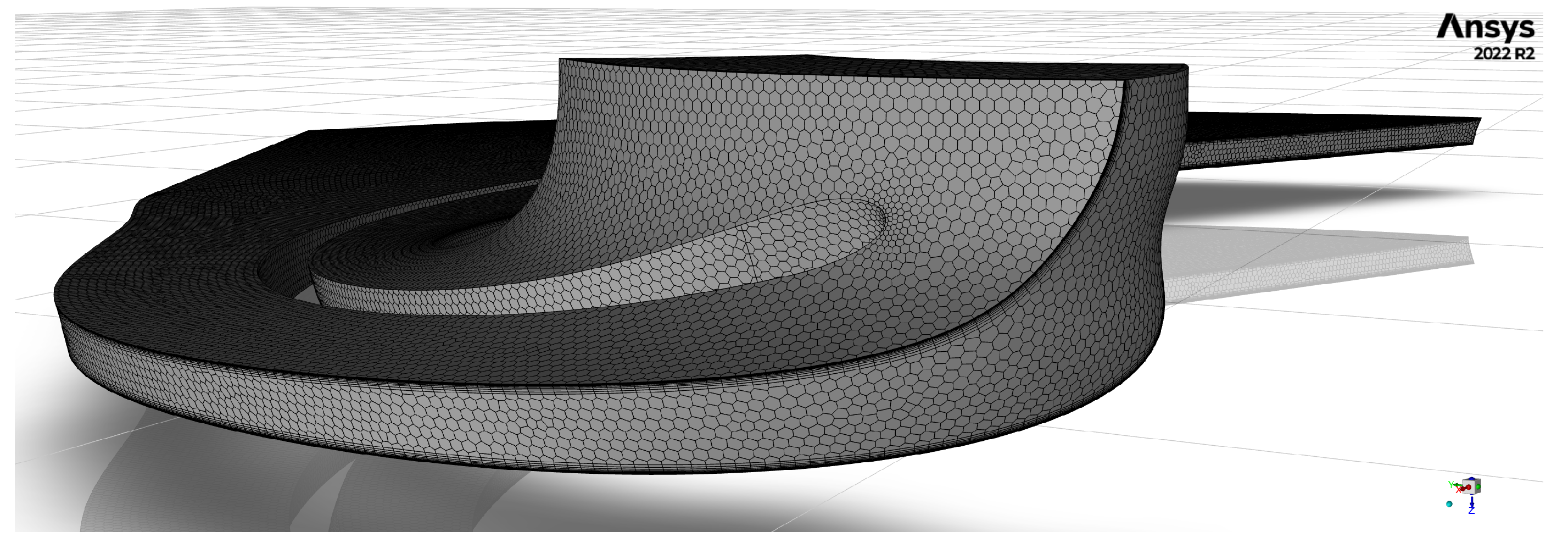
As illustrated in Figure 4, both the impeller torque and the total pressure rise show minimal variations (about $2\%$) across meshes spanning from 80,000 to 850,000 cells. Based on this analysis, the finest mesh is selected for all the subsequent simulations, as it provides improved boundary layer resolution while maintaining a reasonable computational cost (a steady simulation on this mesh requires approximately 10 min of wall-clock time on a 64-core machine equipped with Intel Xeon Gold 6338 processors). For the other geometries in the database, which differ in size, the same grid element dimensions are preserved. The computational mesh is polyhedral and includes 10 inflation layers along the walls with a growth rate of 1.3. In critical regions such as the leading edge of the blade, the local $y^{+}$ varies approximately between 5 and 80. This range spans both the viscous sublayer and the logarithmic region. The Spalart–Allmaras turbulence model in Ansys Fluent has been extended with a $y^{+}$-insensitive wall treatment, which automatically blends the solution between these regions depending on the local $y^{+}$ value [35]. Although the viscous sublayer is not fully resolved throughout the domain and wall functions are applied, this approach is consistent with the implementation of the model in Fluent and appropriate for the preliminary optimization scope of the present work. In fact, the mesh enables accurate prediction of global performance metrics such as total pressure rise across the pump and impeller torque, which are primarily governed by the overall flow field and less sensitive to fine-scale near-wall resolution, as demonstrated by the mesh sensitivity analysis. A visualization of this mesh is provided in Figure 5.

At the end of the high-fidelity calculations, the total pressure and radial velocity fields at the outlet of the domain are extracted and remapped onto a common structured grid defined in non-dimensional angular and axial coordinates. This procedure ensures that data originating from different geometries are projected onto a unified spatial framework, enabling the construction of a reduced-order model based on consistent grid topology.

With this data, it is possible to calculate the mass-weighted average of total pressure at the outlet, which can be expressed as (in the case of constant density) [35]

$$P_{T4,avg}={\displaystyle \frac{{\sum }_{i=1}^{n_i}{P}_{T4,i}·A_{4,i}·\left|c_{m4,i}\right|}{{\sum }_{i=1}^{n_i}{A}_{4,i}·\left|c_{m4,i}\right|}}$$

(9)

where $P_{T4,i}$ is the total pressure value in the i-th cell at the outlet, $A_{4,i}$ is the area of the i-th cell at the outlet, $c_{m4,i}$ is the meridional velocity value in the i-th cell at the outlet, and $n_i$ is the total number of cells on the outlet surface.

Similarly, the radial and tangential velocity fields at the interface between the impeller and the diffuser are remapped onto a common grid to estimate the impeller torque. As discussed by Guelich [9], the torque can be computed either by integrating the pressure and viscous shear stresses over the rotating surfaces (blades, hub, and shroud), or by evaluating the change in angular momentum of the fluid between inlet and outlet. The former approach can be expressed in discretized vector form as

$$\mathbf{T}=\sum _{k=1}^{n_k}{\mathbf{r}}_k\times ({\sigma }_k·{\mathbf{n}}_k)A_k$$

(10)

where ${\mathbf{r}}_k$ is the position vector from the rotation axis to the center of the k-th surface element, $n_k$ is the number of surface elements on the rotating surfaces, ${\sigma }_k$ is the stress tensor on the k-th surface element (including pressure and viscous contributions), $A_k$ is its area, and ${\mathbf{n}}_k$ is the unit normal vector to the surface element. However, remapping the full pressure and wall shear stress distributions along the impeller blades and casing is significantly less practical for ROM construction than remapping the velocity field at the interface. Therefore, the approach based on the change in angular momentum is adopted in this work. Since the inlet flow is normal to the boundary, only the outlet velocity components contribute to the impeller torque. By neglecting the effect of shear stresses at the impeller–diffuser interface due to turbulent exchange of momentum, the torque can be approximated as [9]

$$T\approx \rho ·{\displaystyle \frac{d_2}{2}}·\sum _{j=1}^{n_j}{c}_{u2,j}·c_{m2,j}·A_{2,j}$$

(11)

where $c_{u2,j}$ is the tangential velocity value in the j-th cell at the interface, $c_{m2,j}$ is the meridional velocity value in the j-th cell at the interface, $A_{2,j}$ is the area of the j-th cell at the interface, and $n_j$ is the total number of cells on the interface surface. Even when shear stresses are neglected, Equation (10) still captures the dominant contribution to the torque, whose minimization is a key objective of the optimization process presented in this study. The validity of this assumption is confirmed for the optimal geometry discussed in Section 7.

The remapping procedure is carried out in such a way that the maximum relative error in the quantities specified by Equations (9) and (11) is less than $1\%$ across the entire database when mapping from the original grid to the structured grid.

Examples of remapped results obtained from the CFD calculations are displayed in Figure 6 and Figure 7. These snapshots are then employed to build reduced-order models capable of predicting the flow field within the chosen parameter range, both for the outlet section of the domain and for the interface between the impeller and the diffuser. As anticipated in Section 1, before building the ROMs on all five parameters, the potentiality of reducing the parameter space is explored through the active subspaces technique. This method is outlined in Section 4.

4. Active Subspaces

Many engineering problems involve numerous input parameters, making the computation of a desired output quantity (e.g., for optimization purposes) highly demanding. One possible approach to mitigate this complexity is to investigate whether a reduced set of input variables can still capture the essential behavior of the output function—that is, whether the dimensionality of the parameter space can be effectively reduced. A technique that enables such an analysis is the active subspaces method. This approach was introduced by Russi [36] and developed by Constantine [37]. It has found applications in various fields, including shape optimization in aerodynamics [38] and naval engineering [39], also in conjunction with reduced-order models.

Rather than selecting specific input variables as significant, the active subspaces method focuses on identifying influential directions within the entire input space. Each direction corresponds to a vector of weights that defines a linear combination of the original inputs. If the output of the model remains nearly constant when the inputs vary along one of these directions, that direction can be considered negligible for the purposes of the parameter study [37].

In other words, given a scalar real-valued function f of a vector $\mathbf{x}\in X$, with $X\subseteq {\mathbb{R}}^m$ representing the parameter space, the goal is to identify the orthogonal directions that best capture the variability of f within this space. To do so, the first step is the calculation of the covariance matrix $\mathbf{C}$ of the gradients of f; this matrix can be approximated as [38]

$$\mathbf{C}\approx {\displaystyle \frac{1}{M}}·\sum _{i=1}^M{\nabla }_{\mathbf{x}}{f}_i{\nabla }_{\mathbf{x}}{f}_i^T$$

(12)

where M is the number of sampling points where the gradient of f is evaluated. To identify the most relevant directions, the eigenvectors of $\mathbf{C}$ can be computed; since the covariance matrix is symmetric, it admits a real eigenvalue decomposition:

$$\mathbf{C}=\mathbf{W}\mathbf{\Lambda }{\mathbf{W}}^T$$

(13)

where $\mathbf{W}$ is the matrix of the eigenvectors and $\mathbf{\Lambda }$ is the diagonal matrix of the eigenvalues; both matrices are of dimension $m\times m$. At this point, it is possible to perform the desired dimensionality reduction: with the eigenvalues in decreasing order, $\mathbf{W}$ and $\mathbf{\Lambda }$ can be partitioned as follows:

$$\mathbf{\Lambda }=\left[\begin{array}{cc}{\mathbf{\Lambda }}_{\mathbf{1}}& 0\\ 0& {\mathbf{\Lambda }}_{\mathbf{2}}\end{array}\right],\mathbf{W}=\left[\begin{array}{cc}{\mathbf{W}}_1& {\mathbf{W}}_2\end{array}\right]$$

(14)

where ${\mathbf{\Lambda }}_{\mathbf{1}}$ contains the first n eigenvalues and ${\mathbf{W}}_1$ is made of the first n eigenvectors, with $n<m$. The rationale behind this partitioning is that smaller eigenvalues are associated with directions in which perturbations have less impact in changing the value of f. In this sense, ${\mathbf{W}}_1$ defines the active subspace of the input parameter space; it is thus possible to write

$$f\left(\mathbf{x}\right)\approx g\left({\mathbf{W}}_1^T\mathbf{x}\right)=g\left(\mathbf{y}\right)$$

(15)

where $\mathbf{y}\in {\mathbb{R}}^n$ is the input vector mapped to the active subspace; this resulting vector has a lower dimension compared with the starting vector $\mathbf{x}$.

In this paper, the dimensionality reduction in the parameter space is performed by means of the open source Python package ATHENA [40] (version 0.1.2); the five parameters under study are those listed in Section 2, within the upper and lower bounds outlined in Table 1. Since they are characterized by different orders of magnitude, they are all normalized in the range $[-1,1]$. The first scalar function investigated to assess the presence of an active subspace is the total pressure rise in the pump. This quantity is calculated from the inlet total pressure (which is imposed as a boundary condition) and the mass-weighted average of the outlet total pressure calculated as in Equation (9) from the CFD data. 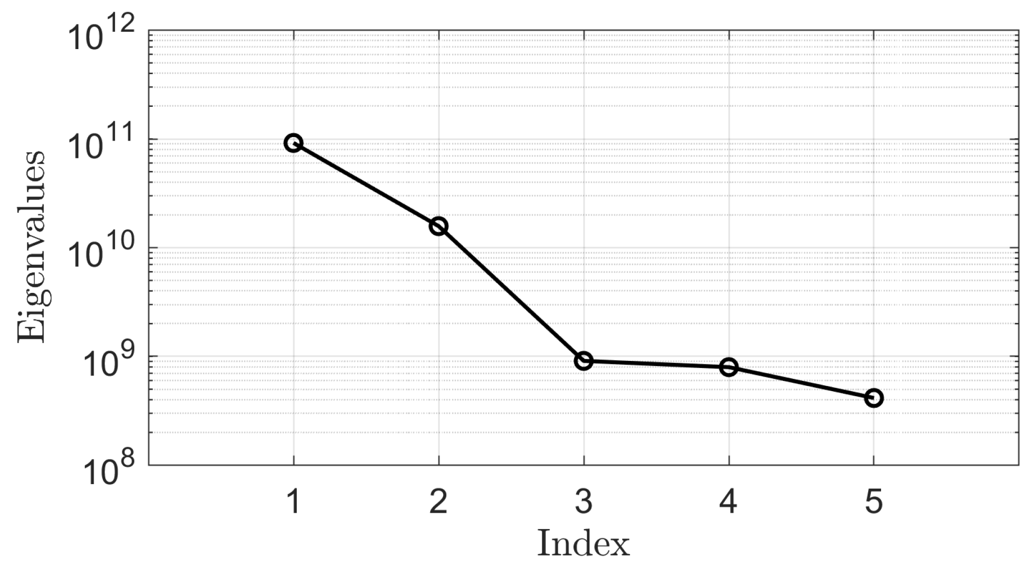The total pressure rise is evaluated for all geometries in the database described in Section 2 and graphically represented in Figure 2. The eigenvalues of the resulting covariance matrix are displayed in Figure 8.

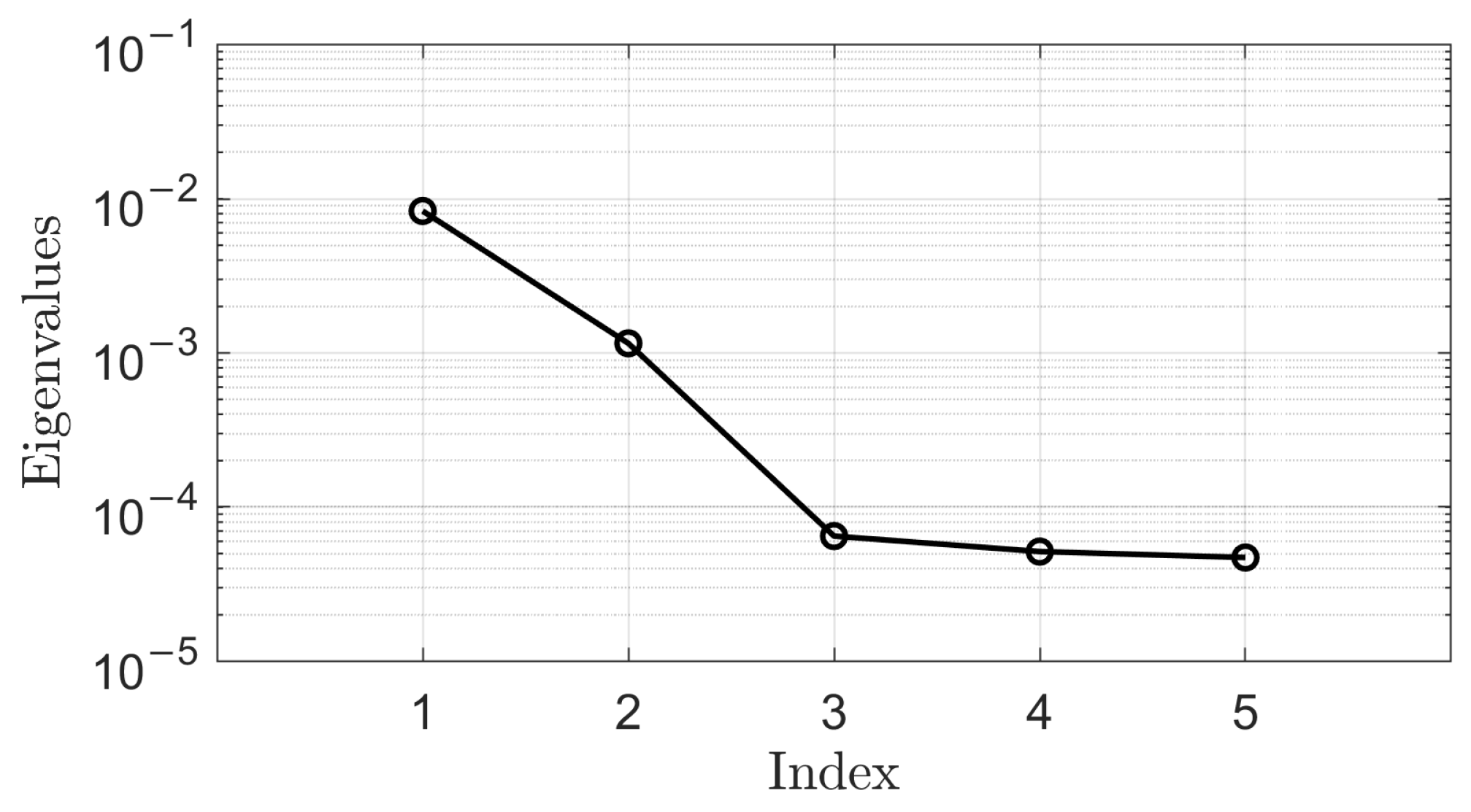
The same procedure is followed for the second scalar function under study, namely the impeller torque, as expressed in Equation (11); the result is shown in Figure 9.

By inspection of Figure 8, it appears that some eigenvalues are several orders of magnitude lower than others; the same consideration can also be performed for Figure 9. To quantify this visual observation, it is common practice to compare the sum of a selected subset of eigenvalues to the total sum, as stated in Ref. [37]. For example, considering the first four eigenvalues yields a ratio of $99.6\%$ for total pressure rise and $99.5\%$ for impeller torque. This means that active subspaces of dimensions lower than that of the original five-dimensional parameter space can be selected to calculate the total pressure rise and the impeller torque with reasonable accuracy. This reduction in dimensionality can be exploited to decrease the cost of the optimization problem. Since the choice of the dimension of the active subspaces is arbitrary, the effect of the size of the parameter vector on the prediction error of the ROM is investigated in Section 6.

5. Reduced-Order Model

While the active subspaces method allows reducing the dimension of the input space (in the case under study, the number of design parameters), the creation of a reduced-order model enables mitigation of the computational cost required for the outputs (i.e., the corresponding values of total pressure rise and impeller torque for each combination of the parameters). Model order reduction usually consists of two phases: in the offline phase, experiments or high-fidelity simulations are performed to gather the empirical data, also called snapshots, necessary to derive the ROM. In the subsequent online phase the ROM can provide significantly faster evaluations of the output quantities compared with the original full-order model (FOM) [21], which is represented by CFD in this study.

As anticipated in Section 1, in this work the reduced-order model is created based on the POD technique; more precisely, on proper orthogonal decomposition with interpolation (PODI) [41]. The central idea is to approximate the solution as an interpolation of the snapshots, each corresponding to a given combination of the input parameters. However, direct interpolation of the original, high-fidelity data can be computationally prohibitive: this is why model order reduction is employed [42]. Thanks to interpolation, the model is capable of also making predictions for a set of parameters that is not included in the initial database. In this paper, all these operations are carried out by means of the open source python library EZyRB [43] (version 1.3.0).

During the offline phase, high-fidelity data—namely the remapped flow fields obtained from CFD simulations, as shown in the examples of Figure 6 and Figure 7—are obtained and stored in the snapshot matrix $\mathbf{S}$. If $n_s$ is the number of snapshots (here, $n_s=100$) and $n_x$ is the number of points in which a flow variable of interest (e.g., total pressure) is evaluated, it is possible to write

$$\mathbf{S}=\left[\begin{array}{c}{\mathbf{s}}_1\\ {\mathbf{s}}_2\\ ⋮\\ {\mathbf{s}}_{n_s}\end{array}\right]\mathrm{with}{\mathbf{s}}_i\in {\mathbb{R}}^{1\times n_x}$$

(16)

where every snapshot ${\mathbf{s}}_i$ corresponds to the field obtained by selecting specified values of the input parameters, contained in the vector ${\mathbf{\mu }}_i$. If $n_p$ is the number of input parameters, the parameter matrix can be written as

$$\mathbf{P}=\left[\begin{array}{c}{\mathit{\mu }}_1\\ {\mathit{\mu }}_2\\ ⋮\\ {\mathit{\mu }}_{n_s}\end{array}\right]\mathrm{with}{\mathit{\mu }}_i\in {\mathbb{R}}^{1\times n_p}$$

(17)

Four distinct ROMs are constructed as a function of the input parameters: two are designed to predict the total pressure and meridional velocity fields at the diffuser outlet—enabling the calculation of the total pressure rise in the pump, the inlet total pressure being fixed—while the remaining two estimate the meridional and tangential velocity fields at the impeller–diffuser interface, from which the impeller torque can be evaluated (as stated in Section 3).

For each of these quantities, singular value decomposition (SVD) is applied to the snapshots matrix:

$$\mathbf{S}=\mathbf{\Psi }\mathbf{\Sigma }{\mathbf{\Phi }}^T$$

(18)

Here, $\mathbf{\Psi }$ denotes the matrix whose columns ${\mathbf{\psi }}_i$ are the left singular vectors—commonly referred to as the POD modes—of the snapshots matrix. The high-fidelity solutions are projected onto this space, allowing them to be expressed as linear combinations of the modes. The corresponding weights in this combination are known as modal coefficients. For a given combination of the input parameters ${\mathit{\mu }}_k$ included in the matrix $\mathbf{P}$, the approximated and high-fidelity solutions (denoted with ${\mathbf{s}}_{reduced}$ and ${\mathbf{s}}_k$, respectively) are equal by construction [44]

$${\mathbf{s}}_k={\mathbf{s}}_{reduced}\left({\mathit{\mu }}_{\mathbf{k}}\right)=\sum _{i=1}^{n_s}{\alpha }_i\left({\mathit{\mu }}_{\mathbf{k}}\right){\mathit{\psi }}_i$$

(19)

Conversely, for a set of input parameters outside of those employed to build the ROM, the POD coefficients ${\alpha }_i$ can be interpolated to calculate the new reduced solution during the online phase. In the present work, this is achieved using radial basis function (RBF) interpolation with a thin plate spline kernel, setting the shape parameter (i.e., the parameter that scales the input to the RBF) equal to 1. Thus, the RBF has the following form:

$$RBF\left(r\right)=r^{2}log\left(r\right)$$

(20)

where r denotes the Euclidean distance between the evaluation point and the center of the RBF. In the aforementioned python library used in this work, the smoothing parameter is set to 0, resulting in exact interpolation through the points employed to build the ROM. All available data points are used (no neighbor restriction). Additionally, a linear polynomial term is automatically included in the interpolation, as required by the thin plate spline kernel to ensure that the problem is well-posed; this corresponds to setting the degree parameter to 1.

Finally, since the singular values ${\sigma }_i$ in matrix $\mathbf{\Sigma }$ associated with the POD modes quantify the contribution of each mode to the reconstruction of the snapshots, the expansion in Equation (19) can be truncated after retaining only the modes that ensure a prescribed level of information. This level can be measured using the relative information content (RIC) indicator, defined as follows (where $\tilde{n}$ denotes the number of retained modes) [21]:

$$RIC\left(\tilde{n}\right)={\displaystyle \frac{{\sum }_{i=1}^{\tilde{n}}{\sigma }_i^2}{{\sum }_{i=1}^{n_s}{\sigma }_i^2}},0\le \tilde{n}\le n_s$$

(21)

As anticipated in Section 4, the dimensionality reduction in the parameter space is also performed for the problem under study. Since, as previously discussed, the choice of the reduced parameter space is arbitrary, an initial reduction from the original five parameters to four modified parameters is considered. Specifically, with reference to Equation (14), the transformation matrix ${\mathbf{W}}_1$ is defined by selecting the first four columns of the matrix $\mathbf{W}$, which is of size $5\times 5$. The matrix ${\mathbf{W}}_1$ thus serves as the mapping from the original parameter space to the reduced one. In particular, because the application of active subspaces yields slightly different results when targeting the total pressure rise across the pump and the impeller torque, two distinct transformation matrices are constructed. One is used to obtain the transformed parameters for building the two ROMs at the outlet (from which the total pressure rise is computed), and the other is used to derive the parameters for the two ROMs at the interface (from which the torque is estimated). In this case, all POD modes are retained (i.e., RIC = 1, or in percentage form, RIC = $100\%$) in the construction of the reduced-order models, in order to preserve the full information content of the snapshot database and achieve the highest possible accuracy in the reconstruction of the flow field.

The accuracy of the reduced-order models is evaluated using the leave-one-out strategy [21]. In this approach, each sampling point is sequentially excluded from the database, and a new POD basis is constructed using the remaining high-fidelity data. This updated basis is then employed to approximate the excluded configuration, providing insight into the ability of the model to reconstruct the flow field from new combinations of the input parameters.

Figure 10 and Figure 11 show the results of the prediction of the reduced-order models with the leave-one-out strategy in the same points of the parameter space displayed in Figure 6 and Figure 7. Visually, the reconstructed fluid dynamic fields exhibit a strong resemblance to the original CFD solutions. To quantitatively assess this similarity, the root mean square error (RMSE) on the total pressure rise and impeller torque is calculated over all ROM predictions. For example, the RMSE on the impeller torque can be computed as follows:

$$\mathrm{RMSE}=\sqrt{{\displaystyle \frac{1}{n_s}}\sum _{i=1}^{n_s}{\left(T_i^{\mathrm{ROM}}-T_i^{\mathrm{CFD}}\right)}^2}$$

(22)

where $T_i^{\mathrm{ROM}}$ is the impeller torque calculated from Equation (11) based on the field predicted by the ROM at the i-th point of the database and $T_i^{\mathrm{CFD}}$ is the same quantity computed from the high-fidelity data of the CFD. With the ROMs built as described above, the resulting RMSE on total pressure rise is $0.6\%$ and that on torque is $2\%$, computed, respectively, with reference to the total pressure rise and torque values obtained from CFD simulations. A rigorous quantitative comparison with other models cited in Section 1 is inherently difficult due to the diversity of modeling strategies, pump geometries, operating conditions, and performance metrics adopted across studies. For instance, Ref. [29] employs an analytical model to estimate pump efficiency as a function of several geometric parameters, reporting an error below $5\%$. Ref. [13], on the other hand, uses a combination of surrogate models to predict input power for varying blade exit angles, achieving an error under $2\%$. However, neither of these approaches reconstructs the full flow field within the pump at critical locations, as the proposed ROMs do. This capability enables the derivation of global performance metrics from localized flow features, offering a physically grounded and computationally efficient alternative for design optimization.

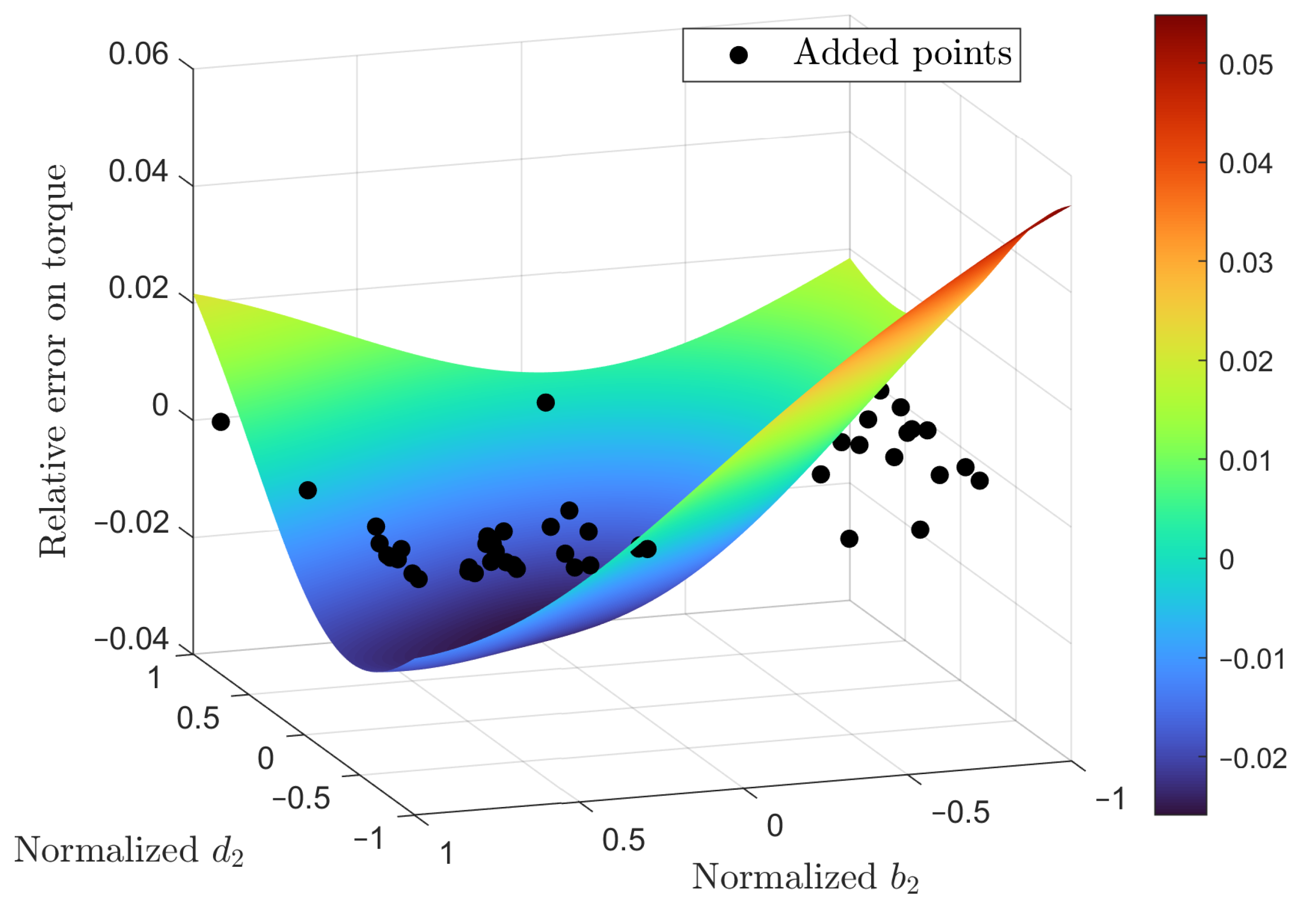
Finally, to assess the adequacy of the initial modeling choices—specifically, the use of four active parameters and a 100-snapshot database without POD mode truncation—Section 6 examines how further adjustments to the parameter space, modal content, and sampling strategy influence the predictive performance of the ROMs.

6. Impact of Parameter Space, Modal Truncation, and Adaptive Sampling

This section investigates how changes in the configuration of the reduced-order models affect their predictive accuracy for the problem under study. Three modifications are considered:

• a further reduction in the dimensionality of the parameter space;
• the truncation of POD modes based on a specified relative information content threshold;
• the enrichment of the snapshot database through adaptive sampling, aimed at improving the ability of the ROMs to capture flow behavior across the design space.

6.1. Effect of Further Dimensionality Reduction in the Parameter Space

The effect on ROM accuracy of reducing the dimensionality of the parameter space can be investigated by mapping the original five parameters onto a further lower-dimensional subspace consisting of only three modified parameters. This can be achieved by selecting the first three columns of the transformation matrix $\mathbf{W}$ of Equation (14), resulting in a reduced matrix ${\mathbf{W}}_1\in {\mathbb{R}}^{5\times 3}$. In this case, the RMSE for the total pressure rise remains unchanged at $0.6\%$, while that for the impeller torque increases to $6\%$, both expressed relative to the corresponding CFD values. This indicates a loss of accuracy for the latter quantity when using a more aggressive dimensionality reduction. As anticipated in Section 4, the selection of the active subspace dimension involves a trade-off between model accuracy and computational efficiency. This trade-off is inherently application-dependent and guided by the desired level of fidelity in the reduced-order model. In the context of this work, where the goal is to demonstrate the feasibility of pump optimization using ROMs coupled with active subspaces, the accuracy of torque prediction is critical. Therefore, the four-dimensional subspace is selected as it represents the minimal reduction that preserves high predictive accuracy ($2\%$ RMSE with respect to CFD), ensuring reliable optimization results while still achieving dimensionality reduction.

6.2. Effect of Modal Truncation Based on Relative Information Content

To evaluate the impact of modal truncation on the precision of the reduced-order models, four new ROMs are constructed by retaining only the number of POD modes required to capture $99.9\%$ of the relative information content. This approach significantly reduces the dimensionality of the reduced space while preserving the dominant structures of the flow. Applying the leave-one-out strategy, the resulting ROM yields RMSE values on total pressure rise and impeller torque ($0.6\%$ and $2.1\%$, respectively, relative to their CFD values) that are virtually unchanged compared with the full-mode ROMs. However, a qualitative analysis of the predicted flow fields reveals that the truncated model is less capable of reproducing localized features of the flow induced by changes in the input parameters. This limitation is illustrated in Figure 12. Compared with Figure 10, which presents the same ROM prediction without truncating the POD basis, it is evident that the overall magnitude and range of the total pressure values are preserved—reflected by the identical colorbar scales—thus confirming the quantitative reliability of the truncated model. Nonetheless, the visual appearance of the predicted flow field differs markedly: the truncated ROM tends to generate smoother, less-detailed structures that appear nearly indistinguishable from one another.

To further investigate the sensitivity of the ROM to modal truncation, additional models are built using more aggressive thresholds of $99.5\%$ and $99.0\%$ RIC. The RMSE on total pressure rise remains stable at approximately $0.6\%$ of its CFD value across all truncation levels, indicating that the dominant pressure features are well captured even with fewer modes. In contrast, the RMSE associated with impeller torque increases relative to the $2.1\%$ observed for the $99.9\%$ RIC model, reaching $4.1\%$ and $3.7\%$ for the $99.5\%$ and $99.0\%$ cases, respectively. This increase does not follow a strictly monotonic trend, suggesting that certain intermediate modes contribute less effectively to torque prediction than those retained at lower RIC values. The number of retained POD modes for each RIC threshold and flow variable is reported in

Table 2. Number of retained POD modes while applying the leave-one-out strategy for different RIC thresholds and flow variables.

	Number of Retained POD Modes
	RIC = 100%	RIC = 99.9%	RIC = 99.5%	RIC = 99%
Outlet total pressure	99	1	1	1
Outlet radial velocity	99	4	2	1
Interface radial velocity	99	7	4	2
Interface tangential velocity	99	3	1	1

. Since all error analyses discussed above are performed using the leave-one-out strategy, and the full dataset contains 100 snapshots, the number of POD modes used at RIC = 100% is 99. With reference to Table 2, the total pressure and radial velocity fields at the outlet are used to compute the total pressure rise in the pump, while the radial and tangential velocity fields at the impeller–diffuser interface are employed to estimate torque, as described in Section 3.

Beyond the aforementioned considerations on prediction error, the full-mode ROM is ultimately selected for optimization in Section 7. Although truncation yields comparable RMSE values for global quantities, it alters the spatial structure of the predicted fields in ways that may compromise the ability of the model to capture localized flow phenomena, potentially leading to suboptimal results.

6.3. Effect of Adaptive Sampling

The original sampling of the parameter space enabled a preliminary exploration aimed at constructing the reduced-order models. In this Subsection, the use of adaptive sampling is introduced in order to automatically refine the initial sampling where the ROM error is larger. To generate the refined database, a radial basis function interpolation is employed to estimate the error on the impeller torque predicted by the original ROM constructed using the four modified parameters with no truncation on POD modes. The RBF is used to interpolate the error, which was previously evaluated by means of the leave-one-out strategy at the original sampling points. The torque error is selected as the target metric for refinement, as its RMSE is higher than that on the total pressure rise. A new Latin hypercube sampling of 5000 points is generated within the parameter space, and the RBF is used to estimate the absolute error at each of these new locations. The points are then ranked according to the absolute value of the error, and the 50 configurations with the highest value are selected for inclusion in the refined database. To ensure diversity and avoid redundancy, a minimum distance criterion is imposed between the newly selected points and those already present in the initial database. The RBF of the error on torque is shown in Figure 13 as a function of normalized values of $d_2$ and $b_2$ in the range $[-1,1]$, with the other three original parameters being fixed. Moreover, the added points are also represented in the normalized $d_2-b_2$ plane.

The transformation matrix for the reduced space with four parameters ${\mathbf{W}}_1\in {\mathbb{R}}^{5\times 4}$ is kept the same as that of Section 5. All ROMs are constructed following the same procedure described above. The leave-one-out strategy is then applied on the refined database consisting of 150 points, in order to assess potential improvements in the predictive capabilities of the model.

Despite the increased number of snapshots, the performance of the ROMs does not exhibit a significant enhancement: the RMSE on total pressure rise remains at $0.6\%$, while the RMSE on impeller torque slightly decreases, becoming equal to $1.9\%$, both computed relative to their respective CFD values. Given the negligible improvement observed when increasing the snapshot database from 100 to 150 samples, and considering the already satisfactory accuracy of the original reduced-order models, the latter are used for carrying out the optimization procedure for the pump, which is the topic of Section 7. This choice ensures computational efficiency while maintaining reliable predictions of the flow field, without requiring a substantially larger sampling effort.

7. Optimization

This section focuses on optimizing the pump geometry by building upon the reduced-order models previously developed using POD with RBF interpolation, and by leveraging the dimensionality reduction achieved through the active subspaces method. As outlined in Section 2, the test case is the ${\mathrm{LH}}_2$ centrifugal pump described by Brewer [1]. The design variables under investigation—$d_2$, $b_2$, ${\beta }_2$, $ϵ$, and Z—are explored within the bounds specified in Table 1. Prior to being input into the ROM, these variables are normalized in the range $[-1,1]$ and then projected onto the four-dimensional parameter space defined in Section 4. The optimization goal is to determine the set of input parameters that minimizes the impeller torque, while satisfying a constraint on the head rise. Specifically, the target head is set to half the value of Brewer’s two-stage pump (i.e., 3755 m at 50,000 rpm and 386 L/min), reflecting the fact that the computational domain includes only a single stage, as illustrated in Figure 3.

The optimization is performed using the Dakota software suite [45] (version 6.22), employing a quasi-Newton method. This algorithm estimates gradients via finite differences, while second-order finite differences serve as an approximation for the Hessian matrix. Both the objective function and the constraint are evaluated using a Python-based analysis driver script, which interfaces with the reduced-order models.

The design variable Z, which can assume only two discrete values within the parameter space, is treated separately to ensure compatibility with the gradient-based optimization algorithm. Specifically, the optimization is performed independently for each fixed value of Z, allowing the remaining continuous variables to be optimized without introducing discontinuities. To mitigate the risk of convergence to local minima, five distinct initial points in the parameter space are generated using Latin hypercube sampling. The resulting optimal values of the design parameters are summarized in

Table 3. Results of the quasi-Newton optimization algorithm.

Design Variables	${\mathit{d}}_2$ [mm]	${\mathit{b}}_2$ [mm]	${\mathit{\beta }}_2$ [°]	$\mathit{ϵ}$ [°]	Z
Best value	96.61	1.79	28.51	137.52	6

.

With the exception of the blade number Z, which is a discrete variable restricted to two admissible values within the design space, $b_2$, ${\beta }_2$ and $ϵ$ exhibit optimal configurations located well within the bounds defined in Table 1. The optimal value of the blade outlet angle ${\beta }_2$ within its admissible range confirms the physical consistency of the model. Specifically, when all other parameters are fixed at their respective optimal values, a lower ${\beta }_2$ fails to meet the target head, while a higher one exceeds the minimum head requirement but increases torque—undesirable for efficiency. This balance supports the reliability of the ROM in capturing key hydraulic trade-offs.

In contrast, the impeller outlet diameter $d_2$ reaches the upper limit of its prescribed range, suggesting that the true optimum may lie beyond the current design space. This observation highlights a potential direction for future exploration, possibly involving an extended parameter domain. However, any extension of the $d_2$ range must also account for non-fluid dynamic constraints: a larger diameter implies higher tip speed, increased rotating mass, and consequent effects on rotor dynamics and bearing loads.

Regarding the performance of the optimized pump geometry, the resulting configuration achieves a hydraulic head of 3755 m, consistent with the target value. The impeller torque, estimated by scaling the torque computed over the periodic sector by the total number of blades, is approximately 3.41 Nm. This corresponds to a hydraulic efficiency of about $85\%$. The relatively high efficiency can be attributed to the fact that the computational domain includes only the internal flow passages of the impeller and diffuser, excluding secondary flow paths and other loss-inducing components present in the complete machine. In particular, the model does not account for disk friction losses—drag losses generated by the side plates of shrouded impellers rotating in a fluid [46]. These losses are particularly significant in low-specific speed pumps [47], such as the one considered in this study. Moreover, secondary flow paths are neglected; their associated losses become non-negligible for pumps operating at low flow rates, as the main flow dimensions are comparable to those of the secondary channels. These simplifications are justified by the scope of the present study, which aims to perform a preliminary optimization of the impeller geometry and demonstrate the feasibility of reduced-order modeling for this purpose.

The accuracy of the results obtained via the quasi-Newton optimization method coupled with the ROMs is validated through a high-fidelity CFD simulation performed on the geometry defined by the optimal combination of design parameters. The simulation settings are consistent with those described in Section 3. The CFD results are computed directly on the original unstructured mesh, without remapping onto the structured grid used to construct the reduced-order models, and thus avoiding interpolation errors that could otherwise affect the comparison. The head obtained from the CFD simulation is 3748 m, exhibiting a deviation of less than $1\%$ compared with the prediction provided by the ROMs. As for the impeller torque, when computed from the high-fidelity CFD simulation using Equation (11), the resulting value is 3.58 Nm, corresponding to a relative error of $4.7\%$ with respect to the ROM prediction. This error is entirely attributable to ROM interpolation, as no POD mode truncation is applied. When frictional effects are additionally considered—i.e., torque is calculated using Equation (10)—the value increases to 3.66 Nm, and the corresponding ROM error rises to $6.8\%$. This error reflects both the interpolation error inherent to the ROM and the contribution from neglecting frictional effects. The limited increase in error upon inclusion of frictional contributions supports the assumption made in Section 3, namely that the dominant component of the torque is captured by Equation (11).

Finally, to further assess whether the quasi-Newton method has identified a global optimum, a multi-objective genetic algorithm (MOGA) is executed, once again using the Dakota software suite. The algorithm is tasked with minimizing the impeller torque and maximizing the head, by varying the design parameters within the bounds specified in Table 1. Genetic algorithms are generally more effective than gradient-based methods in exploring complex parameter spaces, albeit at the cost of a significantly higher number of function evaluations. Given the conflicting nature of the two objectives, the optimization yields a Pareto front—i.e., a set of non-dominated solutions for which improvement in one objective necessarily entails degradation in the other. This result is illustrated in Figure 14, while the main settings of the genetic algorithm are summarized in

Table 4. Main settings of the genetic algorithm for checking the solution of the quasi-Newton method.

Setting	Value
Population Size	50
Max. Function Evaluations	5000
Crossover Rate	0.8
Mutation Rate	0.1

.

As illustrated in Figure 14, the five-blade impeller does not meet the head requirement. On the other hand, with $Z=6$, the constrained optimum identified by the quasi-Newton method lies on the Pareto front. Specifically, among the solutions that yield a head of at least 3755 m, the quasi-Newton method correctly selects the one ensuring the minimum value of torque. Alternative solutions may satisfy the head constraint, but they result in higher impeller torque.

8. Conclusions

In this work, a comprehensive framework for the shape optimization of a centrifugal pump is developed by integrating high-fidelity CFD simulations, reduced-order modeling, and active subspaces. A database of snapshots is collected using Latin hypercube sampling over five geometric design parameters, enabling the construction of reduced-order models capable of predicting the fluid dynamic field at the impeller–diffuser interface and at the pump outlet. From these predictions, key performance metrics such as impeller torque and total pressure rise are derived. Furthermore, the use of POD provides more physical insights with respect to simpler methods based on response surfaces: indeed, the POD does not only provide the integral quantities, but it also reconstructs the flow field, allowing identification of the regions that are related to larger losses. The active subspaces method is employed to reduce the dimensionality of the input parameter space, and a sensitivity analysis is conducted to assess the performances of the ROMs in the case of further dimensional reductions in the input space and POD mode truncation. In addition, an adaptive sampling strategy driven by a leave-one-out error estimate is developed to automatically improve the prediction capabilities of the models. The ROMs are then used to perform geometry optimization via a quasi-Newton algorithm, identifying a set of the design parameters within the prescribed bounds that minimizes impeller torque while satisfying a constraint on the pump head. The correctness of the optimal solution obtained through this process is verified by performing a high-fidelity CFD simulation on the optimized geometry, and by comparing the quasi-Newton result with a multi-objective genetic algorithm, confirming that the identified design lies on the Pareto front and corresponds to a globally optimal trade-off between minimum torque and required head. The results demonstrate the effectiveness of the proposed methodology and highlight the potential of model order reduction strategies in the context of shape optimization for centrifugal pump applications.