Article

A Class of Pursuit Problems in 3D Space via Noncooperative Stochastic Differential Games

School of Astronautics, Harbin Institute of Technology, Harbin 150001, China
*
Author to whom correspondence should be addressed.
These authors contributed equally to this work.
Aerospace 2025, 12(1), 50; https://doi.org/10.3390/aerospace12010050
Submission received: 9 December 2024 / Revised: 31 December 2024 / Accepted: 10 January 2025 / Published: 13 January 2025

Abstract

:
This paper investigates three-dimensional pursuit problems in noncooperative stochastic differential games. By introducing a novel polynomial value function capable of addressing high-dimensional dynamic systems, the forward–backward stochastic differential equations (FBSDEs) for optimal strategies are derived. The uniqueness of the value function under bounded control inputs is rigorously established as a theoretical foundation. The proposed methodology constructs optimal closed-loop feedback strategies for both pursuers and evaders, ensuring state convergence and solution uniqueness. Furthermore, the Lebesgue measure of the barrier surface is computed, enabling the design of strategies for scenarios involving multiple pursuers and evaders. To validate its applicability, the method is applied to missile interception games. Simulations confirm that the optimal strategies enable pursuers to consistently intercept evaders under stochastic dynamics, demonstrating the robustness and practical relevance of the approach in pursuit–evasion problems.

1. Introduction

Motivation: The study of differential game theory has a long and rich history, beginning with the foundational work of Isaacs [1] in the mid-1950s. Over the decades, this field has found applications in diverse domains, such as aerospace, robotics, and control systems [2,3,4,5,6]. A central focus in this area has been the classical non-cooperative linear-quadratic differential game, characterized by linear dynamics and quadratic cost functions. Key advances include necessary and sufficient conditions for the existence of saddle points in deterministic two-player zero-sum differential games over finite time intervals [7]. In stochastic settings, the complexity increases due to uncertainties in system dynamics and decision-making processes. Recent studies have tackled challenges such as unknown system matrices for regulators and participants, leading to adaptive stability solutions for linear-quadratic stochastic differential games [8]. Despite these advances, multi-agent scenarios involving many pursuers and many evaders remain underexplored, particularly in stochastic differential games. Critical challenges include addressing solution uniqueness and quantifying the Lebesgue measure of barrier surfaces, both of which are fundamental to designing optimal strategies.
This paper aims to address these gaps by introducing a novel framework for stochastic differential games in three-dimensional spaces. Specifically, we focus on multi-agent interactions where pursuers and evaders operate under stochastic dynamics. The contributions of this paper are threefold. First, we model these interactions using stochastic differential equations, explicitly accounting for uncertainties to analyze their impact on game strategies. Second, we establish the uniqueness of solutions, ensuring the solvability of the proposed game model. Finally, we compute the Lebesgue measure of the barrier surface using precise mathematical tools, demonstrating its practical relevance in real-world applications such as missile interception.
Brief Summary of Prior Literature: Linear-quadratic differential games have long provided a theoretical foundation for understanding game dynamics under deterministic and stochastic conditions. For games over infinite time horizons, feedback Nash equilibria are well-established, with their existence linked to solutions of algebraic Riccati equations [9]. Extensions to stochastic systems on finite horizons have emphasized feedback information structures, with verification theorems for feedback Stackelberg Nash equilibria derived using fully nonlinear parabolic partial differential equations [10]. Additionally, coupled Riccati equations have been employed to establish local existence, uniqueness, and sufficient conditions for equilibrium solutions. Significant progress has been made in two-player stochastic differential games. For example, Stackelberg solutions under open-loop information structures have been investigated, with applications to mixed linear-quadratic games incorporating input constraints [11]. Similarly, studies on Stackelberg games with Markov jump-diffusion stochastic differential equations have utilized stochastic maximum principles to derive optimal solutions for both leaders and followers [12]. A notable development is the exploration of linear-quadratic Stackelberg differential games for Markov jump-diffusion systems. By formulating a general stochastic maximum principle, open-loop optimal strategies for leaders and followers are derived. The existence of an open-loop saddle point guarantees optimality for both players, as neither can unilaterally improve their outcomes. However, such studies often focus on scenarios involving a single controller in the optimization process. Extensions to multi-agent systems with Markov jump-diffusion dynamics have been investigated by Lv [13], Moon [14], Sun [15], and Zhang and Li [16]. These works analyze interactions between decision-makers under stochastic dynamics but primarily address two-player settings or assume specific structural simplifications.
Recent advancements in multi-agent stochastic differential games have introduced methods such as mean-field games [17] and mixed mean-field analysis [18] to address scenarios with numerous agents. While these approaches offer valuable insights, they often rely on open-loop solutions or simplifying assumptions, such as convex control sets. Feedback strategies, though explored in linear-quadratic frameworks [19], remain underutilized for multi-agent stochastic games involving bounded controls. Studies like [20] have applied the stochastic maximum principle to sequentially solve leader–follower problems, yielding open-loop Stackelberg equilibria. Adaptive strategies for mean-field stochastic differential game problems have been developed using techniques such as weighted least squares estimation, random regularization, and decreasing incentive methods [21]. Additionally, the state-feedback form of Nash equilibrium strategies has been constructed using coupled Riccati equations [22]. Sun and Yong [23] further investigated the properties of open-loop and closed-loop saddle points, while Yu [24] and Miller and Pham [25] extended these approaches to broader scenarios, including McKean–Vlasov stochastic differential equations and Markov jump-diffusion models [26]. Despite these contributions, the challenges of many-to-many stochastic interactions, solution uniqueness, and the impact of bounded controls remain open. This paper extends existing frameworks by employing forward–backward stochastic differential equations (FBSDEs) to model multi-agent interactions. Building on methods from [27,28], we incorporate bounded controls and multi-agent dynamics, addressing both the uniqueness of solutions and the computation of barrier surface measures.
In game theory, Nash equilibrium refers to a situation where all players make decisions simultaneously, and no player can improve their outcome by unilaterally changing their strategy, assuming others keep their strategies unchanged. This concept is widely used in non-hierarchical settings where players have equal decision-making power. On the other hand, Stackelberg equilibrium involves a hierarchical structure. In this scenario, one player (the leader) makes their decision first, while the other players (followers) observe this decision and respond optimally. This sequential decision-making process reflects many real-world scenarios, such as competition between a dominant firm and smaller firms in an industry. The comparison of Nash and Stackelberg Equilibria is shown in Figure 1.
Our work differs from studies by Laszlo and Lions, as well as Carmona, Delarue, and Rachepel, who explored ϵ -mean field games [29]. These works typically assume solvable Riccati equations, simplifying the construction of Stackelberg equilibria. While recent studies have proposed strategies for two-player zero-sum Stackelberg and Nash stochastic linear-quadratic (LQ) games, the relationship between these two types of games remains unclear [30]. Additionally, feedback information structures have been analyzed for Stackelberg games on finite horizons [31], with verification theorems derived from Hamiltonian functions. However, the solvability of Riccati equations remains an open question. Other studies incorporating linear-quadratic partial observation models [32] address correlated states and observation noise but primarily focus on two-player scenarios. In contrast, our study provides a comprehensive framework for addressing multi-agent stochastic differential games. By proving solution uniqueness and computing the Lebesgue measure of barrier surfaces, we address fundamental challenges in the field and broaden its applicability to systems with bounded controls and uncertain dynamics.
Contribution of this paper: Inspired by the above literature, we consider the pursuit problems via the non-cooperative stochastic differential game. The main contributions of this article focus on the following points:
1.
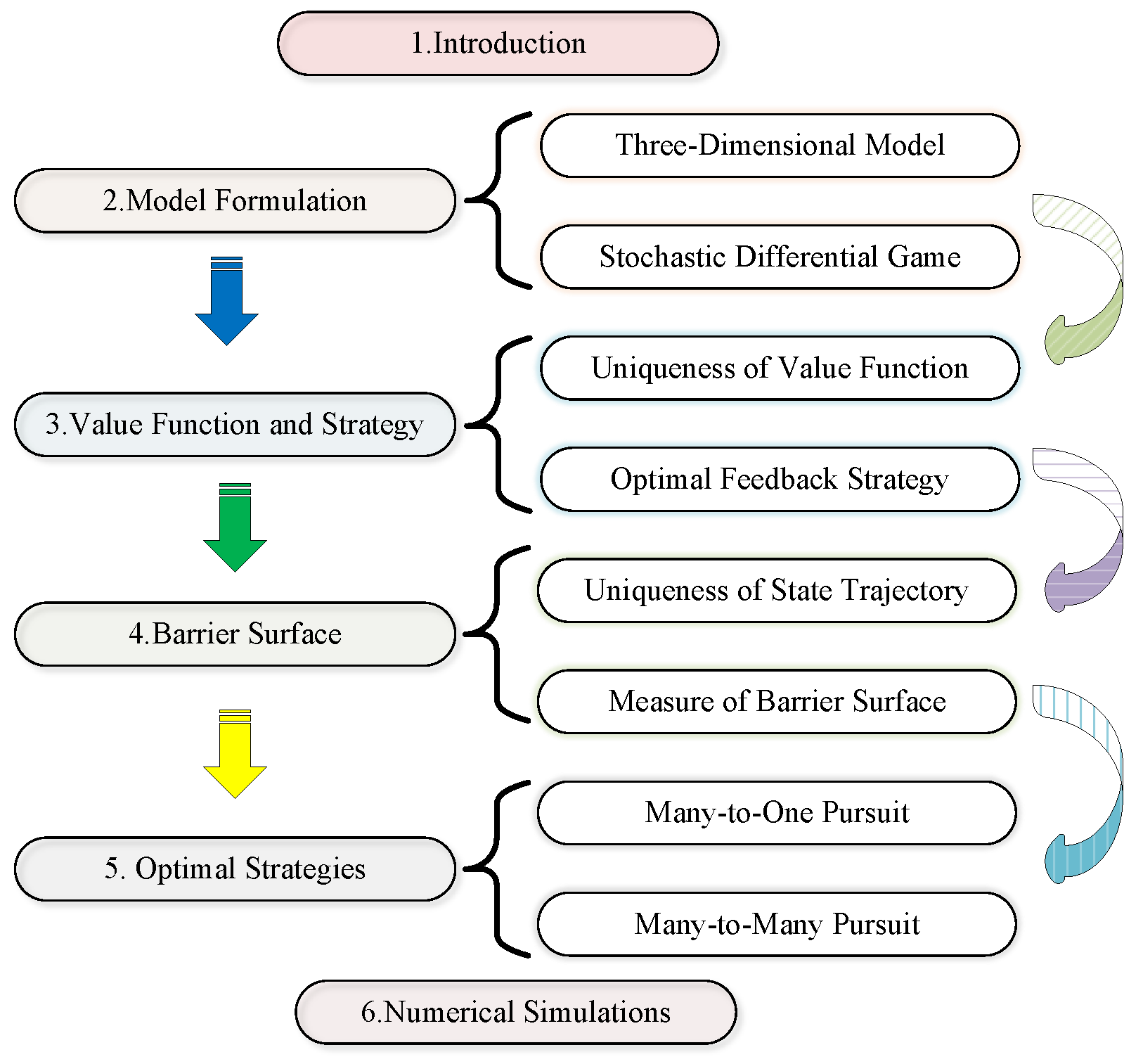
This work extends previous studies (e.g., Qi et al. (2024) in [10]) by addressing pursuit problems in many-to-one and many-to-many scenarios, with initial applications in missile interception. Building on the system dynamics introduced in Section 2.2, we derive the optimal strategies for high-dimensional systems through a system of partial differential equations.
2.
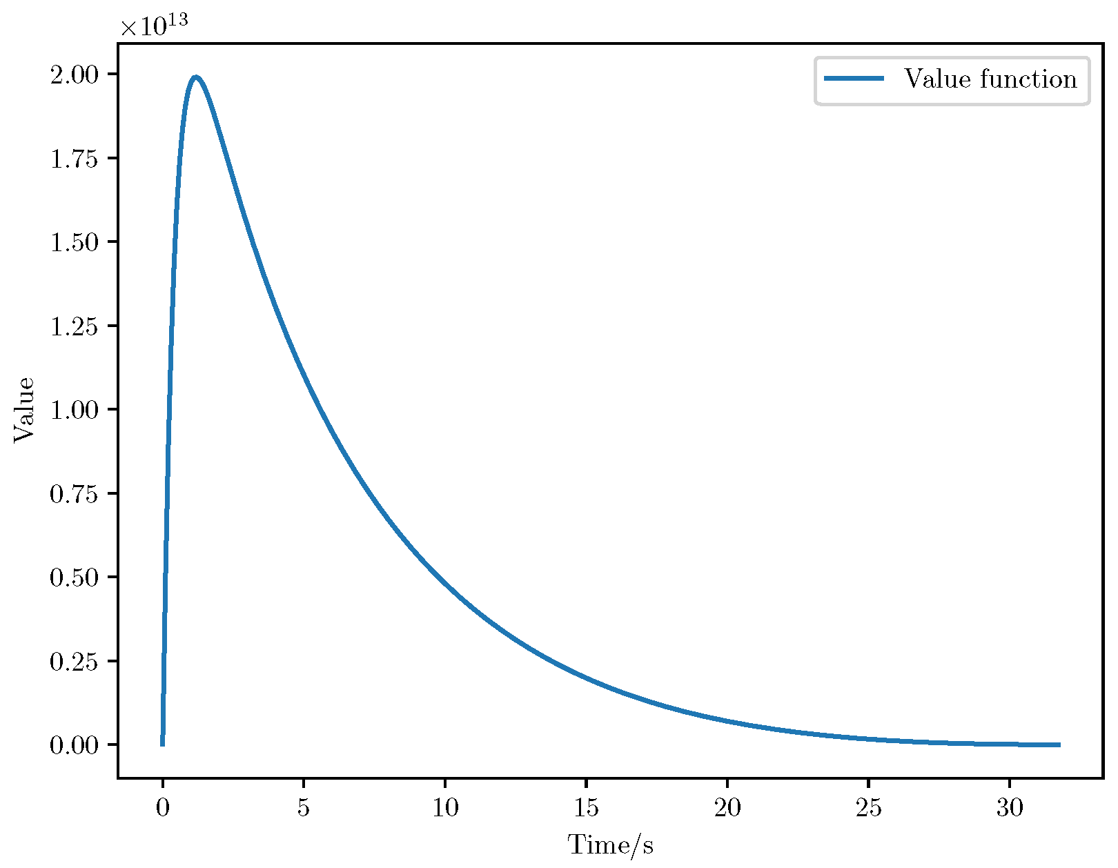
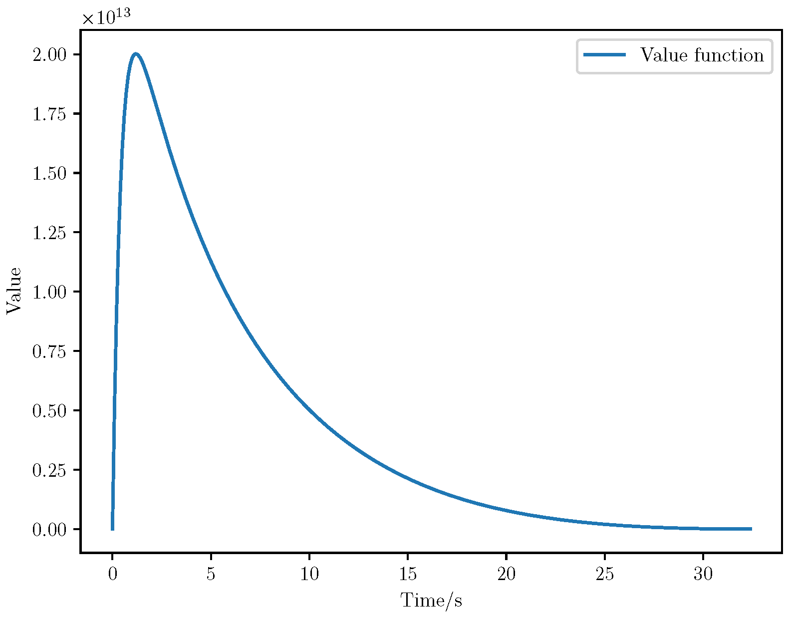
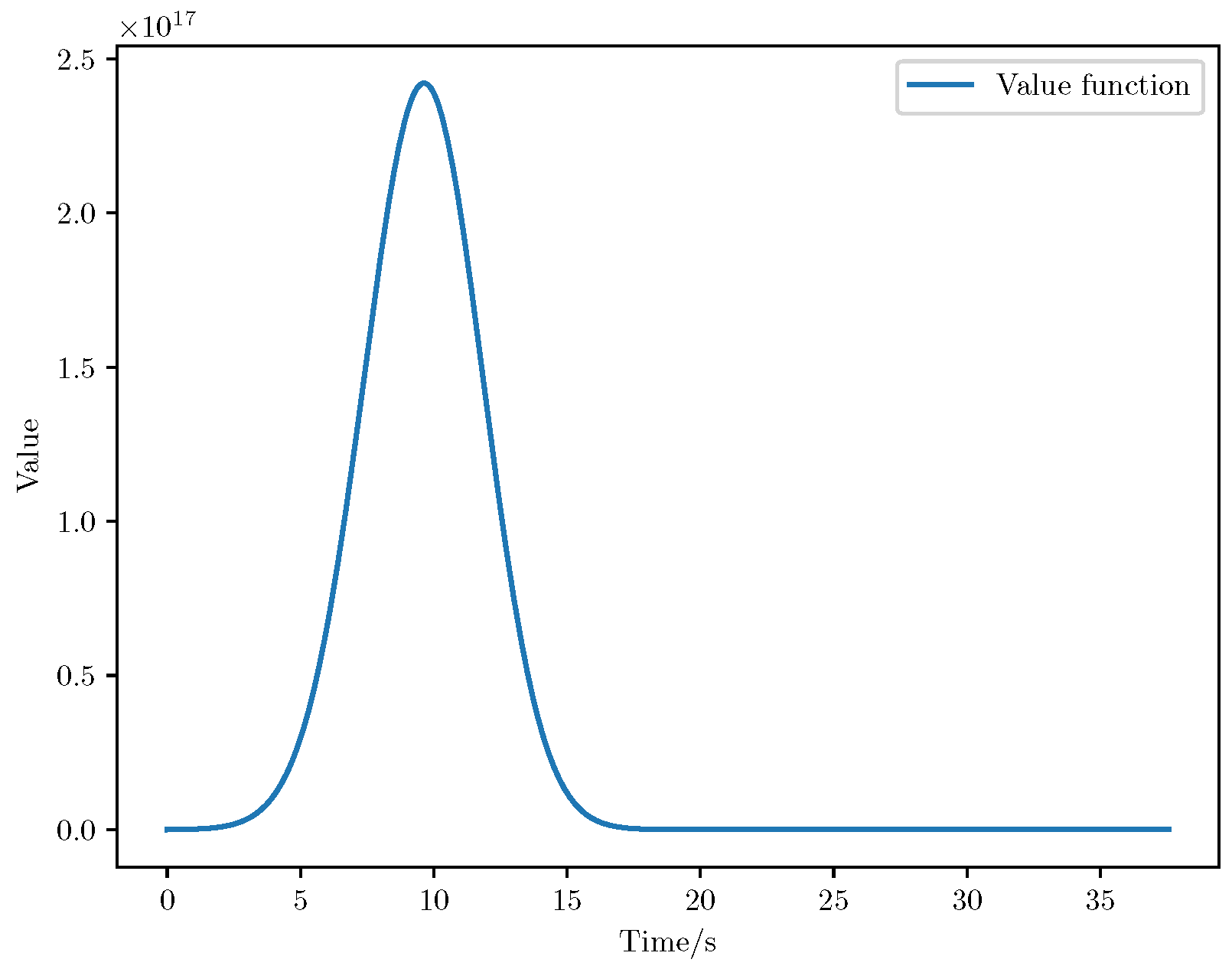
In Section 2 presents a rigorous analysis proving the uniqueness of the value function under bounded control inputs. A novel polynomial value function is introduced, which plays a critical role in ensuring the stability and scalability of the proposed framework.
3.
Leveraging the uniqueness of the value function, we further establish in Section 5 the uniqueness of state trajectories within the pursuit problem. Additionally, we analyze the barrier surface separating the pursuit region and the termination set, demonstrating that its Lebesgue measure is zero. This result is crucial for ensuring the feasibility of optimal strategies in practical scenarios.
The value function chosen in this paper is a polynomial, which differs significantly from the one-dimensional value function discussed in references [10]. This gap leads to distinct solutions and results in the formulation of forward–backward stochastic differential equations (FBSDEs) that are also different from those in [20] in prior works. Specifically, the polynomial nature of the value function necessitates a different approach to solving the system, involving matrix calculations and a more complex formulation of the backward differential equations. Additionally, the method proposed in this paper is applied to high-dimensional systems and, for the first time, is applied to missile interception problems, showcasing its versatility and effectiveness in real-world scenarios.
Through this novel approach, we establish the convergence and uniqueness of the state trajectory when both the pursuer and evader follow the optimal state feedback strategy. Furthermore, we demonstrate that the Lebesgue measure of the barrier surface, which separates the pursuit region from the termination set, is zero. These results, stemming from the novel polynomial form of the value function, contribute new insights to the field of non-cooperative linear-quadratic stochastic differential games.
Organization: The organization of this paper is as follows: In Section 2.1, we introduce a three-dimensional model of the pursuit problem. Based on this model, Section 2.2 formulates a high-dimensional stochastic differential game that incorporates the players’ control variables and the diffusion term of the state equation. In Section 3, we provide proof of the uniqueness of the value function and derive the expression for the optimal closed-loop state feedback strategy. In Section 4, based on the uniqueness of the state trajectory within the pursuit region, the Lebesgue measure of the barrier surface is zero, and the barrier surface consists of points where the rate of distance change is zero. In Section 5, we present optimal strategies for many-to-many pursuit problems. Finally, in Section 6, we validate the feasibility of the optimal strategies designed for many-to-one and many-to-many pursuit problems through numerical simulations. The mind map of this paper is shown in Figure 2.

2. Many-to-One Pursuits Problem in Stochastic Differential Games
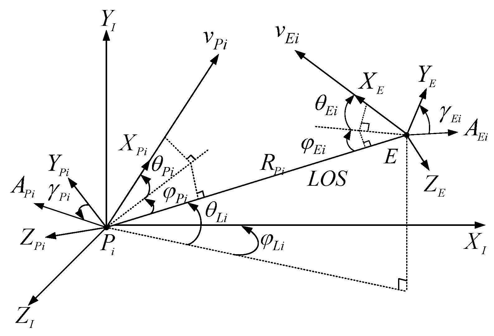
In this section, we will provide a fundamental definition of the many-to-one pursuit problem and present a mathematical model for stochastic differential games. Some assumptions are given.

2.1. Notation

The pursuers P i are collaboratively capturing an evader E i , and the evader is trying to evade the capture of the pursuers. The game is played in a three-dimensional space. Assume that both the pursuers and the evader are mass points with normal acceleration constraints. The direction of the velocity is adjusted by the normal acceleration. The direction of the acceleration is perpendicular to the direction of the velocity. The chase model between a pursuer and an evader is shown in Figure 3. From the above references, the non-linear differential equations are obtained based on the relationship between the pursuer P i and the evader E i in three dimensions [33], i.e.,
R ˙ P i = v E i cos θ E i cos φ E i v P i cos θ P i cos φ P i
R P i θ ˙ L i = v E i sin θ E i v P i sin θ P i
R P i φ ˙ L i cos θ L i = v P i cos θ P i sin φ P i v E i cos θ E i sin φ E i
θ ˙ P i = A y P i v P i + tan θ L i sin φ P i × ( v P i cos θ P i sin φ P i v E i cos θ E i sin φ E i ) R P i + cos φ P i ( v P i sin θ P i v E i sin θ E i ) R P i
φ ˙ P i = A z P i v P i cos θ P i + sin θ P i cos φ P i tan θ L i + v E i cos θ E i sin φ E i v P i cos θ P i sin φ P i R P i cos θ P i sin θ P i sin φ P i v E i sin θ E i v P i sin θ E i R P i cos θ P i v E i cos θ E i sin φ E i v P i cos θ P i sin φ P i R P i
θ ˙ E i = A y E i v E i + tan θ L i sin φ E i × v P i cos θ P i sin φ P i v E i cos θ E i sin φ E i R P i + cos φ E i v P i sin θ P i v E i sin θ E i R P i
φ ˙ E i = A z E i v E i cos θ E i + sin θ E i cos φ E i tan θ L i + v E i cos θ E i sin φ E i v P i cos θ P i sin φ P i R P i cos θ E i sin θ E i sin φ E i v E i sin θ E i v P i sin θ E i R P i cos θ E i v E i cos θ E i sin φ E i v P i cos θ P i sin φ P i R P i
The pursuit–evasion problem in three-dimensional space is modeled with multiple pursuers attempting to capture an evader. The notation used to describe the system dynamics is as follows in Table 1.

2.2. Problem Formulation

In this paper, Ω , F , F t t > 0 , P is a complete probability space, and W s is m-dimensional Brownian motion. For any initial time t > 0 , terminal time T > t , and the initial state x 0 R n , the filtration F t t > 0 is the natural filtration generated by the Brownian motion W ( s ) for t s T , augmented by all the P -null sets of F . According to Equations (1)–(7), we consider a stochastic differential game in a pursuit problem with control input constraints:
d x s = b s , x s + b u 1 x s u 1 s + b u 2 x s u 2 s + b v 1 x s v 1 s + b v 2 x s v 2 s ) d s + σ s , x s , u 1 s , u 2 s , v 1 s , v 2 s d W s , s t , T , x t = x t .
where x ( s ) R m × 1 is the system state with the initial condition x t , m = 5 n + 2 k , n is the number of pursuers, and k is the number of evaders. x = R P 1 , R P 2 , , θ L 1 , φ L 1 , θ L 2 , φ L 2 , θ P 1 , φ P 1 , θ P 2 , φ P 2 , θ E 1 , φ E 1 , T . u 1 ( s ) R n × 1 is the acceleration of pursuers in the velocity coordinate system of the y-axis. u 2 ( s ) R n × 1 is the acceleration of pursuers in the velocity coordinate system of the z-axis. v 1 ( s ) R k × 1 is the acceleration of evader in the velocity coordinate system of the y-axis. v 2 ( s ) R k × 1 is the acceleration of evader in the velocity coordinate system of the z-axis. W s R m × 1 , F t t > 0 , t s T is the standard Wiener process, b ( s , x ( s ) ) R m × 1 , b u 1 ( s , x ( s ) ) R m × n , b u 2 ( s , x ( s ) ) R m × n , b v 1 ( s , x ( s ) ) R m × 1 , b v 2 ( s , x ( s ) ) R m × 1 are real matrices. σ s , x s , u 1 s , u 2 s , v 1 s , v 2 s R m × m is the diffusion term of the system equation. The relevant parameters are illustrated using an example involving three pursuers and two evaders:
1. Matrix b u 1 :
b u 1 = 0 0 0 1 v P 1 0 0 0 0 0 0 1 v P 2 0 0 0 0 0 0 1 v P 3 0 0 0 Start of numbers ( 10 th row )
2. Matrix b u 2 :
b u 2 = 0 0 0 1 v P 1 cos ( θ P 1 ) 0 0 0 0 0 0 1 v P 2 cos ( θ P 2 ) 0 0 0 0 0 0 1 v P 3 cos ( θ P 3 ) 0 0 0 Start of numbers ( 11 th row )
3. Matrix b v 1 :
b v 1 = 0 0 1 v E 1 0 0 0 0 1 v E 2 0 0 Start of numbers ( 16 th row )
4. Matrix b v 2 :
b v 2 = 0 0 1 v E 1 cos ( θ E 1 ) 0 0 0 0 1 v E 2 cos ( θ E 2 ) 0 0 Start of numbers ( 17 th row )
5. Vector b:
b = v E 1 cos θ E 1 cos φ E 1 v P 1 cos θ P 1 cos φ P 1 , v E 1 cos θ E 1 cos φ E 1 v P 2 cos θ P 2 cos φ P 2 , v E 2 cos θ E 2 cos φ E 2 v P 3 cos θ P 3 cos φ P 3 , v E 1 sin θ E 1 v P 1 sin θ P 1 R P 1 , v P 1 cos θ P 1 sin φ P 1 v E 1 cos θ E 1 sin φ E 1 / R P 1 cos θ L 1 , v E 1 sin θ E 1 v P 2 sin θ P 2 R P 2 , v P 2 cos θ P 2 sin φ P 2 v E 1 cos θ E 1 sin φ E 1 / R P 2 cos θ L 2 , v E 2 sin θ E 2 v P 3 sin θ P 3 R P 3 , v P 3 cos θ P 3 sin φ P 3 v E 2 cos θ E 2 sin φ E 2 / R P 3 cos θ L 3 , tan θ L 1 sin φ P 1 ( v P 1 cos θ P 1 sin φ P 1 v E 1 cos θ E 1 sin φ E 1 ) R P 1 + cos φ P 1 ( v P 1 sin θ P 1 v E 1 sin θ E 1 ) R P 1 , sin θ P 1 cos φ P 1 tan θ L 1 + v E 1 cos θ E 1 sin φ E 1 v P 1 cos θ P 1 sin φ P 1 R P 1 cos θ P 1 sin θ P 1 sin φ P 1 v E 1 sin θ E 1 v P 1 sin θ E 1 R P 1 cos θ P 1 v E 1 cos θ E 1 sin φ E 1 v P 1 cos θ P 1 sin φ P 1 R P 1 , tan θ L 2 sin φ P 2 ( v P 2 cos θ P 2 sin φ P 2 v E 1 cos θ E 1 sin φ E 1 ) R P 2 + cos φ P 2 ( v P 2 sin θ P 2 v E 1 sin θ E 1 ) R P 2 , sin θ P 2 cos φ P 2 tan θ L 2 + v E 1 cos θ E 1 sin φ E 1 v P 2 cos θ P 2 sin φ P 2 R P 2 cos θ P 2 sin θ P 2 sin φ P 2 v E 1 sin θ E 1 v P 2 sin θ E 1 R P 2 cos θ P 2 v E 1 cos θ E 1 sin φ E 1 v P 2 cos θ P 2 sin φ P 2 R P 2 , tan θ L 3 sin φ P 3 ( v P 3 cos θ P 3 sin φ P 3 v E 2 cos θ E 2 sin φ E 2 ) R P 3 + cos φ P 3 ( v P 3 sin θ P 3 v E 2 sin θ E 2 ) R P 3 , sin θ P 3 cos φ P 3 tan θ L 3 + v E 2 cos θ E 2 sin φ E 2 v P 3 cos θ P 3 sin φ P 3 R P 3 cos θ P 3 sin θ P 3 sin φ P 3 v E 2 sin θ E 2 v P 3 sin θ E 2 R P 3 cos θ P 3 v E 2 cos θ E 2 sin φ E 2 v P 3 cos θ P 3 sin φ P 3 R P 3 , tan θ L 1 sin φ E 1 ( v P 1 cos θ P 1 sin φ P 1 v E 1 cos θ E 1 sin φ E 1 ) R P 1 + cos φ E 1 ( v P 1 sin θ P 1 v E 1 sin θ E 1 ) R P 1 , sin θ E 1 cos φ E 1 tan θ L 1 + v E 1 cos θ E 1 sin φ E 1 v P 1 cos θ P 1 sin φ P 1 R P 1 cos θ E 1 sin θ E 1 sin φ E 1 v E 1 sin θ E 1 v P 1 sin θ E 1 R P 1 cos θ E 1 v E 1 cos θ E 1 sin φ E 1 v P 1 cos θ P 1 sin φ P 1 R P 1 , tan θ L 3 sin φ E 2 ( v P 3 cos θ P 3 sin φ P 3 v E 2 cos θ E 3 sin φ E 3 ) R P 3 + cos φ E 2 ( v P 3 sin θ P 3 v E 2 sin θ E 2 ) R P 3 , sin θ E 2 cos φ E 2 tan θ L 3 + v E 2 cos θ E 2 sin φ E 2 v P 3 cos θ P 3 sin φ P 3 R P 3 cos θ E 2 sin θ E 2 sin φ E 2 v E 2 sin θ E 2 v P 3 sin θ E 2 R P 3 cos θ E 2 v E 2 cos θ E 2 sin φ E 2 v P 3 cos θ P 3 sin φ P 3 R P 3 ,
6. Pursuer Inputs u 1 and u 2 :
u 1 = A y P 1 A y P 2 A y P 3 , u 2 = A z P 1 A z P 2 A z P 3
7. Evader Inputs v 1 and v 2 :
v 1 = A y E 1 A y E 2 , v 2 = A z E 1 A z E 2
The cost function of the pursuers and the evader is as follows:
J ( u , v ) = E t T e t s c ( r ) d r x T C x + u T D u v T Δ v d s + e t T c ( r ) d r x T ( T ) R T x ( T )
where e t s c r d r is the discounting function, and c r is the function of time. C R m × m , D R 2 n × 2 n , Δ R 2 × 2 , R T R m × m , u = [ u 1 , u 2 ] T , v = [ v 1 , v 2 ] T , D = D 1 D 2 , Δ = Δ 1 Δ 2 , D , Δ is the orthogonal matrix.
Assumption 1. 
For the convenience of subsequent calculations of the cost function J u , v , it is assumed that [9]:
  • L s , x , u 1 , u 2 , v 1 , v 2 = x T C x + u T D u v T Δ v , g x = x s T R T x s . There exist positive constants C L , C g , and p 2 such that:
e t s c x r d r L s , x , u 1 , u 2 , v 1 , v 2 C L 1 + x p + u 1 p + u 2 p + v 1 p + v 2 p
e t s c x r d r g x C g 1 + x p
Assumption 2. 
It could be assumed that B = b + b u 1 u 1 + b u 2 u 2 + b v 1 v 1 + b v 2 v 2 , and σ is continuous and bounded. There exist positive constants C b , C u , C σ , C b σ such that [18]:
B s , x , u 1 , u 2 , v 1 , v 2 B s , y , u 1 , u 2 , v 1 , v 2 C b x y
B s , x , u 1 , u 2 , v 1 , v 2 B s , x , u ¯ 1 , u ¯ 2 , v ¯ 1 , v ¯ 2 C u u 1 u ¯ 1 p + u 2 u ¯ 2 p + v 1 v ¯ 1 p + v 2 v ¯ 2 p
σ s , x , u 1 , u 2 , v 1 , v 2 σ s , y , u 1 , u 2 , v 1 , v 2 C σ x y
B s , x , u 1 , u 2 , v 1 , v 2 + σ s , x , u 1 , u 2 , v 1 , v 2 C b σ 1 + x
where s [ t , T ] . x , y R n . The admissible control sets for pursuers and evader could be defined as follows:
U = u i u i t , T × R n × 1 , u i is uniformly locally Lipschitz continuous , u i ( s , x ) u i max , i = 1 , 2 .
ν = v i v i t , T × R n , v i is uniformly locally Lipschitz continuous , v i ( s , x ) v i max , i = 1 , 2 .
for all s t , T , L s , x , u 1 , u 2 , v 1 , v 2 and g ( x ) is continuously differentiable. In the missile interception model presented in this paper, we assume that the control inputs are bounded. Specifically, the trajectory control engine, which governs the missile’s movement, has an upper limit on its output, which is related to the normal acceleration. This assumption is crucial for modeling practical missile systems, where limitations on engine power and physical constraints on acceleration are common.
This assumption of bounded control inputs is supported by previous works in the field. For instance, references [34,35] provide theoretical justification for such constraints in control systems, while references [36,37] discuss their applicability to missile interception problems. Moreover, reference [38] highlights the impact of input constraints on system stability and performance, further validating the choice of this assumption in our model.

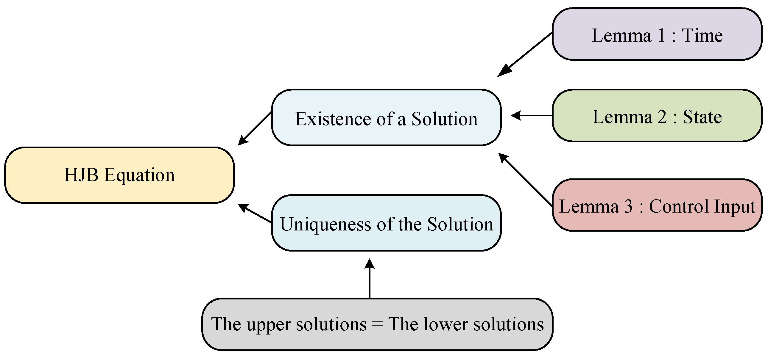
3. The Optimal Feedback Strategies

Definition 1. 
The triple strategy u i * , v i * U , ν , i = 1 , 2 is called to constitute a Nash equilibrium if the triple strategy is within the admissible control set, and if the following hold:
min u i * U J u 1 * , u 2 * , v 1 , v 2 min u i * U max v i * ν J u 1 * , u 2 * , v 1 * , v 2 * max v i * ν J u 1 , u 2 , v 1 * , v 2 *
for any s , x t , T × R m . In this context, the pursuer aims to minimize the profit function, whereas the evader seeks to maximize it.
min u U max v ν J = E t T e t s c ( r ) d r x T C s x + u T D u v T Δ v d s + e t T c ( r ) d r x ( T ) T R T x ( T )
For the second term of the cost function, A matrix p R m × m is a solution for the terminal term,
d p = α d s + β d W = A T p + ζ x E ( x ) d s + β d W
where p T = R T , α = A T p + ζ x E ( x ) , ζ ( x ) is a function that depends on the state, ζ ( 0 ) = 0 .   β is a stochastic diffusion term. Applying Itô’s Lemma to compute p T x T , x T
x T T R T x T = p T x T , x T = p t x t , x t + t T x T α x + x T p B + B T p x + 2 σ T β x + t r p σ σ T d s + t T x T β x + 2 σ T p x d W .
Combining (19) and (21), the following could be obtained:
J = E e t s c r d r t T x T C s x + u T D s u v T D s v d s + e t s c r d r x T R x = E e t s c r d r t T x T C s x + u T D s u v T D s v + x T α x + 2 B T p x + 2 σ T β x + t r p σ σ T d s + e t s c r d r t T β x T x + 2 p σ T x d W + e t s c r d r p t x t , x t .
The second term of the cost function (22) is equal to zero, and the third term is relative to the initial state, such that
J = E e t s c r d r t T x T C s x + u T D s u v T D s v d s + e t s c r d r x T R x = E t T e t s c r d r x T C s x + u T D s u v T D s v + x T α x + 2 B T p x + 2 σ T β x + t r p σ σ T d s .
In this paper, the H J B -equation for Ψ s , x = inf u i U sup v i ν J s , x becomes:
s Ψ + inf u i U sup v i ν 1 2 t r σ s σ * s x x 2 Ψ + b s , x Ψ + c Ψ + L = 0 , s t , T .
Theorem 1. 
the value function Ψ t , x C 1 , 2 t , T × R m is the classical solution of HJB, u i * , v i * U , ν , u i s , x u i max , v i s , x v i max , i = 1 , 2 . such that Ψ , s Ψ , x Ψ , x x 2 Ψ C Ψ 1 + x N , for some N 0 . If ( x * , u 1 * , u 2 * , v 1 * , v 2 * ) is an admissible pair at t , x , F c v = 1 2 t r σ s σ * s x x 2 Ψ + b s , x Ψ + c Ψ + L , such that u 1 * , u 2 * , v 1 * , v 2 * arg inf u i U sup v i n u F c v . For almost everywhere, s t , T . Then, the pair ( x * , u 1 * , u 2 * , v 1 * , v 2 * ) is optimal at t , x .
Proof. 
Based on Itô’s Lemma:
Ψ s , x = E Ψ T , x t T s Ψ + b , x Ψ + 1 2 t r σ s σ * s x x 2 Ψ d s
Then, the following could be obtained:
J t , x , u 1 * , u 2 * , v 1 , v 2 E g x T t T s Ψ L + F c v Ψ + Ψ d s J t , x , u 1 , u 2 , v 1 * , v 2 * .
If and only if F c v = Ψ , Ψ t , x = J t , x , u 1 , u 2 , v 1 , v 2 . If u 1 , u 2 , v 1 , v 2 = u 1 * , u 2 * , v 1 * , v 2 * , then the equation above gives: Ψ t , x = V t , x = J t , x , u 1 * , u 2 * , v 1 * , v 2 * , where value function V t , x is the viscosity solution of the HJB equation. It may be the case that a continuous first and second derivative C 1 , 2 does not exist. □
Step 1: the value function V t , x is the Lipschitz continuous function.
Proof. 
We introduce three Lemmas 1–3, to complete the proof. To prove that the value function is Lipschitz continuous, it is necessary to demonstrate that each input parameter of the value function satisfies the Lipschitz continuity condition. This step ensures the mathematical rigor of the subsequent solution process. While the numerical simulations in this paper are conducted within the R 3 space, the uniqueness of the value function as a solution holds true in higher-dimensional spaces as well. We provide a simplified overview of the lemmas used:
  • Lemma 1: Proves that time is Lipschitz continuous, ensuring stability with respect to temporal variations.
  • Lemma 2: Shows that the state is Lipschitz continuous, accounting for the relationship between states and dynamics.
  • Lemma 3: Demonstrates that the control inputs are Lipschitz continuous under bounded constraints, ensuring consistency of input–output relationships.
These lemmas collectively establish the Lipschitz continuity of the value function, providing a foundation for the uniqueness proof in both low- and high-dimensional spaces.
Lemma 1. 
For any s [ t , T ] , x 1 , x 2 R m , there exists C λ 1 , C λ 2 , such that:
inf u i U E C λ 1 x 1 x 2 p V t , x 1 , u 1 , u 2 , v 1 , v 2 V t , x 2 , u 1 , u 2 , v 1 , v 2 sup v i ν E C λ 2 x 1 x 2 p .
V t is Lipschitz continuous.
Proof. 
For any s [ t , T ] , we can obtain the following:
x 1 s = x 1 t + t s B s , x 1 d s + t s σ s , x 1 d W . x 2 s = x 2 t + t s B s , x 2 d s + t s σ s , x 2 d W .
Then,
x 1 s x 2 s = x 1 t x 2 t + t s B s , x 1 B s , x 2 d s + t s σ s , x 1 σ s , x 2 d W .
Taking expectations on both sides of the equation:
E x 1 ( s ) x 2 ( s ) E x 1 ( t ) x 2 ( t ) + t s C b x 1 x 2 d s
According to the Gronwall inequality, there exists a positive constant C b such that:
E x 1 s x 2 s E e C b s t x 1 t x 2 t
for any s t T , such that:
E x 1 s x 2 s E e C b T x 1 t x 2 t
ε > 0 , x 1 , x 2 R n , such that:
V t , x 2 , u 1 , u 2 , v 1 , v 2 + ε sup v i ν E t T e t s c r d r L s , x 1 , u 1 , u 2 , v 1 , v 2 d s + e t s c r d r g x T
V t , x 1 , u 1 , u 2 , v 1 , v 2 V t , x 2 , u 1 , u 2 , v 1 , v 2 ε sup v i ν E t T e t s c r d r L s , x 1 , u 1 , u 2 , v 1 , v 2 L s , x 2 , u 1 , u 2 , v 1 , v 2 d s + e t s c r d r g x 1 T e t s c r d r g x 2 T
There exist constants C L and C g , such that:
V t , x 1 , u 1 , u 2 , v 1 , v 2 V t , x 2 , u 1 , u 2 , v 1 , v 2 ε sup v i ν E t T C L x 1 x 2 p d s + C g x 1 T x 2 T p sup v i ν E C L e C b T x 1 x 2 p T + C g e C b T x 1 x 2 p sup v i ν E C λ x 1 x 2 p .
Similarly, we could obtain the following:
inf u i U E C λ 1 x 1 x 2 p V t , x 1 , u 1 , u 2 , v 1 , v 2 V t , x 2 , u 1 , u 2 , v 1 , v 2 sup v i ν E C λ 2 x 1 x 2 p
where C λ is a constant, which depends on T , C L , C b , C g . This completes the proof of Lemma 1. □
Lemma 2. 
For any x R m , V x is Lipschitz continuous. There exist constants k 1 , k 2 , such that:
inf u i U E k 2 1 + x P T V t 1 , x t 1 V t 2 , x t 1 sup v i ν E k 1 1 + x P T .
Proof. 
t 1 t 2 , t 1 , t 2 0 , T .
x t 2 x t 1 = t 1 t 2 B s , x d s + t 1 t 2 σ s , x d W
Then,
E x t 2 x t 1 = E t 1 t 2 B s , x d s .
We could obtain the following:
E B t , x , u 1 , u 2 , v 1 , v 2 B t , 0 , u 1 , u 2 , v 1 , v 2 E C b x , E B t , x , u 1 , u 2 , v 1 , v 2 E B t , 0 , u 1 , u 2 , v 1 , v 2 + C b x E max v i ν B t , 0 , u 1 , u 2 , v 1 , v 2 + C b x E M F + C b x ,
where M F : = max v i ν B 0 , u 1 , u 2 , v 1 , v 2 .
E min u i U B 0 , u 1 , u 2 , v 1 , v 2 C b x E B x , u 1 , u 2 , v 1 , v 2
where m F : = min u i U B 0 , u 1 , u 2 , v 1 , v 2 . Then, x R n , t 1 , t 2 0 , T .
V t 1 , x = inf u i U sup v i ν E t 1 t 1 + h e t s c r d r L s , x , u 1 , u 2 , v 1 , v 2 d s + V t 2 , x
where h = t 2 t 1 . The following could be obtained:
V t 1 , x t 1 V t 2 , x t 1 V t 2 , x t 2 V t 2 , x t 1 + sup v i ν E t 1 t 2 e t s c r d r L s , x , u 1 , u 2 , v 1 , v 2 d s E C λ x t 2 x t 1 p + sup v i ν E t 1 t 2 e t s c r d r L s , x , u 1 , u 2 , v 1 , v 2 d s          sup v i ν E C λ M F + C b x P T + M L + C M x P T sup v i ν E k 1 1 + x P T .
On the other hand, for any δ > 0 , such that:
V t 1 , x t 1 V t 2 , x t 1 + δ V t 2 , x t 2 V t 2 , x t 1 + inf u i U E t 1 t 2 e t s c r d r L s , x , u 1 , u 2 , v 1 , v 2 d s inf u i U E k 2 1 + x P T .
Then, let δ 0 . We can obtain the following:
inf u i U E k 1 + x P T V t 1 , x t 1 V t 2 , x t 1 sup v i ν E k 1 + x P T .
This completes the proof of Lemma 2. □
Then, we need to add a proof regarding the impact of bounded inputs on value functions.
Lemma 3. 
u 1 , u 2 , u ¯ 1 , u ¯ 2 U , u ¯ i = u max , v 1 , v 2 , v ¯ 1 , v ¯ 2 ν , v ¯ i = v max , there exist constants C L 1 , C L 2 , such that:
inf u i U E C L 1 e C u T T u 1 u ¯ 1 p + u 2 u ¯ 2 p + v 1 v ¯ 1 p + v 2 v ¯ 2 p V t , x , u 1 , u 2 , v 1 , v 2 V t , x , u ¯ 1 , u ¯ 2 , v ¯ 1 , v ¯ 2 sup v i ν E C L 2 e C u T T u 1 u ¯ 1 p + u 2 u ¯ 2 p + v 1 v ¯ 1 p + v 2 v ¯ 2 p .
Proof. 
s t , T , x R N , there exists a constant C L 1 , such that:
V t , x , u 1 , u 2 , v 1 , v 2 V t , x , u ¯ 1 , u ¯ 2 , v ¯ 1 , v ¯ 2 sup v i ν E t T e C e s L s , x , u 1 , u 2 , v 1 , v 2 L s , x , u ¯ 1 , u ¯ 2 , v ¯ 1 , v ¯ 2 d s sup v i ν E t T C L 1 1 + u 1 u ¯ 1 p + u 2 u ¯ 2 p + v 1 v ¯ 1 p + v 2 v ¯ 2 p d s sup v i ν E C L 1 e C u T T u 1 u ¯ 1 p + u 2 u ¯ 2 p + v 1 v ¯ 1 p + v 2 v ¯ 2 p .
Then, there exists a constant C L 2 , such that:
V t , x , u 1 , u 2 , v 1 , v 2 V t , x , u ¯ 1 , u ¯ 2 , v ¯ 1 , v ¯ 2 sup v i ν E t T e C e s L s , x , u 1 , u 2 , v 1 , v 2 L s , x , u ¯ 1 , u ¯ 2 , v ¯ 1 , v ¯ 2 d s sup v i ν E t T C L 1 + u 1 u ¯ 1 p + u 2 u ¯ 2 p + v 1 v ¯ 1 p + v 2 v ¯ 2 p d s sup v i ν E C L e C u T T u 1 u ¯ 1 p + u 2 u ¯ 2 p + v 1 v ¯ 1 p + v 2 v ¯ 2 p .
This completes the proof of Lemma 3. □
According to Lemmas 1–3, we can obtain the following:
V t 1 , x 1 , u 1 , u 2 , v 1 , v 2 V t 2 , x 2 , u ¯ 1 , u ¯ 2 , v ¯ 1 , v ¯ 2 V t 1 , x 1 , u 1 , u 2 , v 1 , v 2 V t 1 , x 2 , u 1 , u 2 , v 1 , v 2 + V t 1 , x 2 , u 1 , u 2 , v 1 , v 2 V t 2 , x 2 , u 1 , u 2 , v 1 , v 2 + V t 2 , x 2 , u 1 , u 2 , v 1 , v 2 V t 2 , x 2 , u ¯ 1 , u ¯ 2 , v ¯ 1 , v ¯ 2 .
Then, we could obtain the following:
inf u i U E C L 1 e C u T T u 1 u ¯ 1 p + u 2 u ¯ 2 p + v 1 v ¯ 1 p + v 2 v ¯ 2 p + C λ 1 x 1 x 2 p + k 1 1 + x P T V t 1 , x 1 , u 1 , u 2 , v 1 , v 2 V t 2 , x 2 , u ¯ 1 , u ¯ 2 , v ¯ 1 , v ¯ 2 sup v i ν E C L e C u T T u 1 u ¯ 1 p + u 2 u ¯ 2 p + v 1 v ¯ 1 p + v 2 v ¯ 2 p + C λ x 1 x 2 p + k 1 + x P T .
This completes the proof of step 1. □
Step 2: the value function V t , x is the unique viscosity solution of the H J B equation.
Proof. 
We assume that V 1 is a sub-solution. Let μ be the standard complete probability space: μ = Ω 1 , F , F s t , P , where W η is a Wiener process in the filtration probability space Ω , F , F s t , P . Here, F is the augmentation by P -sets, and F s t is the σ -algebra generated by W η .
J t , x , u 1 , u 2 , v 1 , v 2 = E t t + h e t s c r d r L s , x , u 1 , u 2 , v 1 , v 2 d s + E t + h T e t s c r d r L s , x , u 1 , u 2 , v 1 , v 2 d s + e t s c r d r g x T | F t + h T = E t t + h e t s c s d r L s , x , u 1 , u 2 , v 1 , v 2 d s + E E t + h T e t + h s c s d r L s , x , u 1 , u 2 , v 1 , v 2 d s + e t s c s d r g x T | F t + h T = E t t + h e t s c s d r L s , x , u 1 , u 2 , v 1 , v 2 d s + E e t + h s c r d r J u t + h , x , u 1 , u 2 , v 1 , v 2 + ς E t t + h L s , x , u 1 , u 2 , v 1 , v 2 d s + inf u i U e t + h T c r d r V 1 t + h , x , u 1 , u 2 , v 1 , v 2 .
Then, we can obtain the following:
inf u i U V 1 t , x , u 1 , u 2 , v 1 , v 2 E t t + h e t s c r d r L s , x , u 1 , u 2 , v 1 , v 2 d s + inf u i U e t + h T c r d r V t + h , x , u 1 , u 2 , v 1 , v 2 . inf u i U V 1 t , x , u 1 , u 2 , v 1 , v 2 inf u i U e t + h T c r d r V 1 t + h , x , u 1 , u 2 , v 1 , v 2 E t t + h e t + h T c r d r L s , x , u 1 , u 2 , v 1 , v 2 d s . E t t + h e C e s L s , x , u 1 , u 2 , v 1 , v 2 d s + inf u i U e t + h T c r d r V 1 t + h , x , u 1 , u 2 , v 1 , v 2 inf u i U V 1 t , x , u 1 , u 2 , v 1 , v 2 0 . inf u i U V 1 t , x , u 1 , u 2 , v 1 , v 2 inf u i U e t + h T c r d r V 1 t + h , x , u 1 , u 2 , v 1 , v 2 E t t + h e t + h s c r d r L s , x , u 1 , u 2 , v 1 , v 2 d s 0 .
For any t 0 , x 0 t , T × R n , and there exists Ψ 1 C 1 , 2 ( t , T × R n ) , with V 1 Ψ 1 attaining its maximum at t 0 , x 0 , we have:
e t + h T c r d r V 1 t , x e t + h T c r d r Ψ 1 t , x V 1 t 0 , x 0 Ψ 1 t 0 , x 0
where t 0 , x 0 t , T × R n .
e t 0 + h T c r d r V 1 t 0 + h , x 0 e t 0 + h T c r d r Ψ 1 t 0 + h , x 0 + h V 1 t 0 , x 0 Ψ 1 t 0 , x 0 .
Ψ 1 t 0 , x 0 e t 0 + h T c r d r Ψ 1 t 0 + h , x 0 + h V t 0 , x 0 e t 0 + h T c r d r V t 0 + h , x 0 .
Ψ 1 t 0 , x 0 e t 0 + h T c r d r Ψ 1 t 0 + h , x 0 + h E t 0 t 0 + h e t 0 s c r d r L s , x , u 1 , u 2 , v 1 , v 2 d s 0 .
Then, we can obtain the following:
inf u i U E 1 h t 0 t 0 + h e t 0 s c r d r s Ψ 1 e t 0 s c r d r B T x Ψ 1 e t 0 s c r d r 1 2 σ s T σ s x x 2 Ψ 1 1 e t 0 s c r d r Ψ 1 e t 0 s c r d r L d s 0 .
lim h 0 s Ψ 1 + inf u i U B T x Ψ 1 + 1 2 σ s T σ s T x x 2 Ψ 1 + C e Ψ 1 + L 0 .
where C e = lim h 0 e t 0 t 0 + h c r d r 1 h . Similarly, V 2 is a supersolution. For any t 0 , x 0 t , T × R m , there exists Ψ 2 C 1 , 2 ( t , T × R n ) , such that V 2 Ψ 2 attains a minimum at t 0 , x 0 , and we have V 2 t , x Ψ 2 t , x V 2 t 0 , x 0 Ψ 2 t 0 , x 0 . Then, we have the following: s Ψ 2 + sup v i ν ( B x Ψ 2 + 1 2 ( σ s T σ s ) T x x 2 Ψ 2 + C e Ψ 2 + L ) 0 . Next, we prove the existence of a unique solution V to ensure that the HJB equation has a unique solution. Let M : = sup t 0 , T { V 1 V 2 } . Assuming by contradiction that M > 0 , we construct the following function using the doubling variable technique: for ε , β , χ > 0 and 0 < m 1 < 1 .
Φ t 1 , x 1 , u 1 , u 2 , v 1 , v 2 , t 2 , x 2 , u 1 , u 2 , v 1 , v 2 = V 1 t 1 , x 1 , u 1 , u 2 , v 1 , v 2 V 2 t 2 , x 2 , u 1 , u 2 , v 1 , v 2 t 1 t 2 p + x 1 x 2 p p ε β 1 + x 1 p + 1 + x 2 p m 1 χ u 1 u 1 + u 2 u 2 + v 1 v 1 + v 2 v 2
where Φ is continuous and the last three terms of equation (54) are used to estimate the discontinuities. When
Φ ( t 1 , x 1 , u 1 , u 2 , v 1 , v 2 , t 2 , x 2 , u 1 , u 2 , v 1 , v 2 ) ,
then max x 1 , x 2 . Then, the following exists:
sup Φ t 1 , x 1 , u 1 , u 2 , v 1 , v 2 , t 2 , x 2 , u 1 , u 2 , v 1 , v 2 = Φ t ¯ 1 , x ¯ 1 , u ¯ 1 , u ¯ 2 , v ¯ 1 , v ¯ 2 , t ¯ 2 , x ¯ 2 , u ¯ 1 , u ¯ 2 , v ¯ 1 , v ¯ 2 .
According to the definition of M, there exists ( t ˜ , x ˜ , u ˜ 1 , u ˜ 2 , v ˜ 1 , v ˜ 2 ) , such that:
V 1 t ˜ , x ˜ , u ˜ 1 , u ˜ 2 , v ˜ 1 , v ˜ 2 V 2 t ˜ , x ˜ , u ˜ 1 , u ˜ 2 , v ˜ 1 , v ˜ 2 M 2
Then:
Φ t ¯ 1 , x ¯ 1 , u ¯ 1 , u ¯ 2 , v ¯ 1 , v ¯ 2 , t ¯ 2 , x ¯ 2 , u ¯ 1 , u ¯ 2 , v ¯ 1 , v ¯ 2 Φ t ˜ , x ˜ , u ˜ 1 , u ˜ 2 , v ˜ 1 , v ˜ 2 , t ˜ , x ˜ , u ˜ 1 , u ˜ 2 , v ˜ 1 , v ˜ 2 V 1 t ˜ , x ˜ , u ˜ 1 , u ˜ 2 , v ˜ 1 , v ˜ 2 V 2 t ˜ , x ˜ , u ˜ 1 , u ˜ 2 , v ˜ 1 , v ˜ 2 2 β 1 + x ˜ p m 1 χ u ˜ 1 u ˜ 1 + u ˜ 2 u ˜ 2 + v ˜ 1 v ˜ 1 + v ˜ 2 v ˜ 2 M 2 2 β 1 + x ˜ p m 1 .
There exist β R , such that β 1 + x ˜ p m 1 = M 8 . Then:
Φ t ¯ 1 , x ¯ 1 , u ¯ 1 , u ¯ 2 , v ¯ 1 , v ¯ 2 , t ¯ 2 , x ¯ 2 , u ¯ 1 , u ¯ 2 , v ¯ 1 , v ¯ 2 M 4 .
We can obtain the following:
V 1 t ¯ 1 , x ¯ 1 , u ¯ 1 , u ¯ 2 , v ¯ 1 , v ¯ 2 V 2 t ¯ 2 , x ¯ 2 , u ¯ 1 , u ¯ 2 , v ¯ 1 , v ¯ 2 M 4 β 1 + x ¯ 1 p + 1 + x ¯ 2 p m 1
V 1 and V 2 are bound, then there exists a constant C x , such that:
β 1 + x ¯ 1 p + 1 + x ¯ 2 p m 1 C x
According to this assumption, we can obtain the following:
t ¯ 1 t ¯ 2 p + x ¯ 1 x ¯ 2 p p ε V 1 t ¯ 1 , x ¯ 1 , u ¯ 1 , u ¯ 2 , v ¯ 1 , v ¯ 2 V 1 t ¯ 2 , x ¯ 2 , u ¯ 1 , u ¯ 2 , v ¯ 1 , v ¯ 2 + V 2 t ¯ 1 , x ¯ 1 , u ¯ 1 , u ¯ 2 , v ¯ 1 , v ¯ 2 V 2 t ¯ 2 , x ¯ 2 , u ¯ 1 , u ¯ 2 , v ¯ 1 , v ¯ 2
We assume the existence of a continuity modulus ω :
t ¯ 1 t ¯ 2 p + x ¯ 1 x ¯ 2 p p ε 2 ω t ¯ 1 t ¯ 2 + x ¯ 1 x ¯ 2 + u ¯ 1 u ¯ 1 + u ¯ 2 u ¯ 2 + v ¯ 1 v ¯ 1 + v ¯ 2 v ¯ 2
According to the state bounded, control inputs are strictly bounded, t ¯ 1 t ¯ 2 C ε , x ¯ 1 x ¯ 2 C ε . u ¯ 1 u ¯ 1 + u ¯ 2 u ¯ 2 + v ¯ 1 v ¯ 1 + v ¯ 2 v ¯ 2 4 C ε , we can obtain the following:
t ¯ 1 t ¯ 2 p + x ¯ 1 x ¯ 2 p p ε 2 ω 6 p ε ,
χ u 1 u 1 + u 2 u 2 + v 1 v 1 + v 2 v 2 4 χ C ε .
Next, we assume:
ϕ 1 = V 2 t 2 , x 2 , u 1 , u 2 , v 1 , v 2 + t 1 t 2 p + x 1 x 2 p p ε + β 1 + x 1 p + 1 + x 2 p m 1 + χ u 1 u 1 + u 2 u 2 + v 1 v 1 + v 2 v 2 .
ϕ 2 = V 1 t 1 , x 1 , u 1 , u 2 , v 1 , v 2 t 1 t 2 p + x 1 x 2 p p ε β 1 + x 1 p + 1 + x 2 p m 1 χ u 1 u 1 + u 2 u 2 + v 1 v 1 + v 2 v 2 .
Incorporateing the above Equations (62)–(64) into the Equations (65) and (66), the following could be obtained:
s ϕ 1 + inf u i U B T x ϕ 1 + 1 2 σ s T σ s T x x 2 ϕ 1 + C e V 1 + L = | t 1 t 2 | p 1 ε + C e V 1 ( t 1 ¯ , x 1 ¯ ) + B T | x 1 x 2 | p 1 ε + β m 1 1 + | x 1 | p + 1 + | x 2 | p m 1 1 p | x 1 | p 1 2 1 + | x 1 | p + 1 2 σ s T σ s T | x 1 x 2 | p 2 ( p 1 ) ε + β m 1 ( m 1 1 ) 1 + | x 1 | p + 1 + | x 2 | p m 1 2 p | x 1 | p 1 2 1 + | x 1 | p + β m 1 1 + | x 1 | p + 1 + | x 2 | p m 1 1 p ( p 1 ) | x 1 | p 2 2 1 + | x 1 | p p | x 1 | p 1 2 1 + | x 1 | p 2 + L 0 .
We could obtain the following:
s ϕ 2 + sup v i ν B x ϕ 2 + 1 2 σ s T σ s x x 2 ϕ + C e V 2 + L = | t 1 t 2 | p 1 ε + C e V 2 ( t 2 ¯ , x 2 ¯ ) + B T | x 1 x 2 | p 1 ε + β m 1 1 + | x 1 | p + 1 + | x 2 | p m 1 1 p | x 2 | p 1 2 1 + | x 2 | p + 1 2 σ s T σ s T | x 1 x 2 | p 2 ( p 1 ) ε + β m 1 ( m 1 1 ) 1 + | x 1 | p + 1 + | x 2 | p m 1 2 p | x 2 | p 1 2 1 + | x 2 | p + β m 1 1 + | x 1 | p + 1 + | x 2 | p m 1 1 p ( p 1 ) | x 2 | p 2 2 1 + | x 2 | p p | x 2 | p 1 2 1 + | x 2 | p 2 + L 0 .
Subtracting the above two Equations (67) and (68) yields the following:
C e V 1 ( t 1 ¯ , x 1 ¯ ) V 2 ( t 2 ¯ , x 2 ¯ ) + B T x 1 x 2 p 1 ε + β m 1 1 + x 1 p + 1 + x 2 p m 1 1 p x 1 p 1 2 1 + x 1 p + 1 2 ( σ s T σ s ) T x 1 x 2 p 2 ( p 1 ) ε + β m 1 ( m 1 1 ) 1 + x 1 p + 1 + x 2 p m 1 2 p x 1 p 1 2 1 + x 1 p + β m 1 1 + x 1 p + 1 + x 2 p m 1 1 p ( p 1 ) x 1 p 2 2 1 + x 1 p p x 1 p 1 p x 1 p 1 2 1 + x 1 p ( 2 1 + x 1 p ) 2 B T x 1 x 2 p 1 ε + β m 1 1 + x 1 p + 1 + x 2 p m 1 1 p x 2 p 1 2 1 + x 2 p 1 2 ( σ s T σ s ) T x 1 x 2 p 2 ( p 1 ) ε + β m 1 ( m 1 1 ) 1 + x 1 p + 1 + x 2 p 1 2 p x 2 p 1 2 1 + x 2 p + β m 1 1 + x 1 p + 1 + x 2 p m 1 1 p ( p 1 ) x 2 p 2 2 1 + x 2 p p x 2 p 1 p x 2 p 1 2 1 + x 2 p ( 2 1 + x 2 p ) 2 0 .
For the second term of Equation (69):
B T x 1 x 2 p 1 ε + β m 1 1 + x 1 p + 1 + x 2 p m 1 1 p x 2 p 1 2 1 + x 2 p B T x 1 x 2 p 1 ε β m 1 1 + x 1 p + 1 + x 2 p m 1 1 p x 1 p 1 2 1 + x 1 p
= B T β m 1 1 + x 1 p + 1 + x 2 p m 1 1 p x 2 p 1 2 1 + x 2 p p x 1 p 1 2 1 + x 1 p
Then:
= B T β m 1 1 + x 1 p + 1 + x 2 p m 1 1 p x 2 p 1 2 1 + x 2 p p x 1 p 1 2 1 + x 1 p = B T β m 1 1 + x 1 p + 1 + x 2 p m 1 1 C p x 2 x 1
for the third term of Equations (69) and (70).
1 2 σ s T σ s T x 1 x 2 p 2 ( p 1 ) ε + β m 1 ( m 1 1 ) 1 + x 1 p + 1 + x 2 p m 1 2 × p x 2 p 1 2 1 + x 2 p + β m 1 1 + x 1 p + 1 + x 2 p m 1 1 × p ( p 1 ) x 2 p 2 2 1 + x 2 p p x 2 p 1 p x 2 p 1 2 1 + x 2 p 2 1 + x 2 p 2 1 2 σ s T σ s T x 1 x 2 p 2 ( p 1 ) ε + β m 1 ( m 1 1 ) 1 + x 1 p + 1 + x 2 p m 1 2 × p x 1 p 1 2 1 + x 1 p + β m 1 1 + x 1 p + 1 + x 2 p m 1 1 × p ( p 1 ) x 1 p 2 2 1 + x 1 p p x 1 p 1 p x 1 p 1 2 1 + x 1 p 2 1 + x 1 p 2
There exists constant C p and C p 2 , such that:
1 2 σ s T σ s T β m 1 ( m 1 1 ) 1 + x 1 p + 1 + x 2 p m 1 2 × C p x 2 x 1 + β m 1 1 + x 1 p + 1 + x 2 p m 1 1 × C p 2 x 2 x 1
Therefore, we can obtain the following:
C e V 1 t ¯ 1 , x ¯ 1 V 2 t ¯ 2 , x ¯ 2 B T β m 1 + x 1 p + 1 + x 2 p m 1 1 × C p x 2 x 1 + 1 2 σ s T σ s T β m 1 ( m 1 1 ) 1 + x 1 p + 1 + x 2 p m 1 2 × C p x 2 x 1 + β m 1 1 + x 1 p + 1 + x 2 p m 1 1 × C p 2 x 2 x 1
C e M 4 B T β m 1 1 + x 1 p + 1 + x 2 p m 1 1 × C p x 2 x 1 + 1 2 σ s T σ s T β m 1 ( m 1 1 ) 1 + x 1 p + 1 + x 2 p m 1 2 × C p x 2 x 1 + β m 1 1 + x 1 p + 1 + x 2 p m 1 1 × C p 2 x 2 x 1
Let β 0 , and assume that C e > 0 . Under this assumption, we obtain M 0 , which contradicts the initial assumption that M > 0 . Therefore, we conclude that: M = sup t 0 , T V 1 V 2 0 . This implies: V 1 V 2 . Similarly, if V 1 is a viscosity supersolution and V 2 is a viscosity subsolution, we can deduce that: V 1 V 2 . Thus, it can be concluded that: V 1 = V 2 . This shows that when the control input is strictly bounded, the value function is the unique viscosity solution of the Hamilton–Jacobi–Bellman (HJB) equation. □
Viscosity solutions may not have first- or second-order continuity. Given that the problem involves stochastic elements, we introduce functions Ψ 1 and Ψ 2 to approximate V 1 and V 2 , respectively, which allows us to represent the Hamilton–Jacobi–Bellman (HJB) equation. By using Ψ 1 Ψ 2 to approximate V 1 V 2 , we avoid dealing with the discontinuities of V 1 and V 2 directly. Specifically, Formulas (65) and (66) allow us to remove the non-differentiable points of V 1 and V 2 through the introduction of boundedness conditions. Our ultimate goal is to prove that the upper bound of V 1 V 2 is less than zero, thereby confirming that V 1 V 2 . A similar proof can be used to show V 1 V 2 .
We provide a detailed explanation of the derivation process for the HJB equation as a solution. To demonstrate the existence of a unique solution, two aspects must be addressed: Existence of a solution: The existence of a solution is established by proving that the value function is Lipschitz continuous. Uniqueness of the solution: The uniqueness of the solution is proven using a contradiction method. Specifically, by showing that the upper and lower solutions converge to the same value, we confirm the uniqueness of the solution. To support these points, we use Lemmas 1–3: Lemma 1 demonstrates that time is Lipschitz continuous. Lemma 2 establishes that the state is Lipschitz continuous. Lemma 3 confirms that under bounded control inputs, the control inputs are Lipschitz continuous. The derivation process for the HJB equation is shown in the Figure 4.
Next, we proceed to solve the H J B equation. Let Ψ ( t , x ) be the value function that solves the H J B equation. The solution takes the following form:
Ψ s , x = x T S 1 x + S 2 T x + x T S 3 + S 4
where S 1 R m × m with S 1 ( T ) = 0 , S 2 R m × 1 with S 2 ( T ) = 0 , S 3 R m × 1 with S 3 ( T ) = 0 , and S 4 R 1 × 1 with S 4 ( T ) = 0 . Using Equation (75), we obtain the following:
f ( s , x ) = x T S 1 x + ( S 2 ) T x + x T S 3 + S 4 + e t s c ( r ) d r x T C x + u T D u v T Δ v + x T α x + x T p B + B T p x + β T σ x + x T σ β + tr ( p σ T σ ) + C e x T S 1 x + S 2 T x + x T S 3 + S 4 + B T S 1 x + S 1 T x + S 2 + S 3 + i , j ( σ s σ s T ) i , j S 1 , i , j
where S 1 = d d s S 1 , S 2 = d d s S 2 , S 3 = d d s S 3 , S 4 = d d s S 4 . According to the first-order condition optimality, the optimal feedback strategy could be expressed as follows:
u 1 * = D 1 1 e t s c r d r 2 b u 1 T S 1 x + S 1 T x + S 2 + S 3 + b u 1 T p x , u 2 * = D 2 1 e t s c r d r 2 b u 2 T S 1 x + S 1 T x + S 2 + S 3 + b u 2 T p x , v 1 * = Δ 1 1 e t s c r d r 2 b v 1 T S 1 x + S 1 T x + S 2 + S 3 b v 1 T p x , v 2 * = Δ 2 1 e t s c r d r 2 b v 2 T S 1 x + S 1 T x + S 2 + S 3 b v 2 T p x .
Next, by incorporating the optimal strategies from Equation (77) into the H J B Equation (24), we can compare the quadratic, linear, and constant terms. This leads to the following coupled Riccati equations:
S 1 + e t s c ( r ) d r ( α + C ) + C e S 1 + e t s c ( r ) d r 4 S 1 T b u 1 D 1 b u 1 T S 1 + e t s c ( r ) d r 4 S 1 T b u 1 D 1 S 1 T + 1 2 S 1 T b u 1 D 1 b u 1 T p + e t s c ( r ) d r 4 S 1 D 1 b u 1 T S 1 + e t s c ( r ) d r 4 S 1 D 1 S 1 T + 1 2 S 1 D 1 b u 1 T p + 1 2 p T b u 1 D 1 b u 1 T S 1 + 1 2 p T b u 1 D 1 S 1 T + e t s c ( r ) d r p T b u 1 D 1 b u 1 T p + e t s c ( r ) d r 4 S 1 T b u 2 D 2 b u 2 T S 1 + e t s c ( r ) d r 4 S 1 T b u 2 D 2 S 1 T + 1 2 S 1 T b u 2 D 2 b u 2 T p + e t s c ( r ) d r 4 S 1 D 2 b u 2 T S 1 + e t s c ( r ) d r 4 S 1 D 2 S 1 T + 1 2 S 1 D 2 b u 2 T p + 1 2 p T b u 2 D 2 b u 2 T S 1 + 1 2 p T b u 2 D 2 S 1 T + e t s c ( r ) d r p T b u 2 D 2 b u 2 T p e t s c ( r ) d r 4 S 1 T b v 1 Δ 1 b v 1 T S 1 e t s c ( r ) d r 4 S 1 T b v 1 Δ 1 S 1 T + 1 2 S 1 T b v 1 D 1 b v 1 T p e t s c ( r ) d r 4 S 1 Δ 1 b v 1 T S 1 e t s c ( r ) d r 4 S 1 Δ 1 S 1 T + 1 2 S 1 Δ 1 b v 1 T p + 1 2 p T b v 1 Δ 1 b v 1 T S 1 + 1 2 p T b v 1 Δ 1 S 1 T e t s c ( r ) d r x T p T b v 1 Δ 1 b v 1 T p x e t s c ( r ) d r 4 S 1 T b v 2 Δ 2 b v 2 T S 1 e t s c ( r ) d r 4 S 1 T b v 2 Δ 2 S 1 T + 1 2 S 1 T b v 2 D 2 b v 2 T p e t s c ( r ) d r 4 S 1 Δ 2 b v 2 T S 1 e t s c ( r ) d r 4 S 1 Δ 2 S 1 T + 1 2 S 1 Δ 2 b v 2 T p + 1 2 p T b v 2 Δ 1 b v 2 T S 1 + 1 2 p T b v 2 Δ 2 S 1 T e t s c ( r ) d r x T p T b v 2 Δ 2 b v 2 T p x = 0 .
where S 1 T = 0 .
S 2 T + e t s c ( r ) d r 4 S 2 + S 3 T D 1 b u 1 T S 1 + e t s c ( r ) d r 4 S 2 + S 3 T D 1 b u 1 T S 1 T + 1 2 S 2 + S 3 T D 1 b u 1 T p + e t s c ( r ) d r 4 S 2 + S 3 T D 2 b u 2 T S 1 + e t s c ( r ) d r 4 S 2 + S 3 T D 2 b u 2 T S 1 T + 1 2 S 2 + S 3 T D 2 b u 2 T p + e t s c ( r ) d r 4 S 2 + S 3 T Δ 1 b v 1 T S 1 + e t s c ( r ) d r 4 S 2 + S 3 T Δ 1 b v 1 T S 1 T + 1 2 S 2 + S 3 T Δ 1 b v 1 T p + e t s c ( r ) d r 4 S 2 + S 3 T Δ 2 b v 2 T S 1 + e t s c ( r ) d r 4 S 2 + S 3 T Δ 2 b v 2 T S 1 T + 1 2 S 2 + S 3 T Δ 2 b v 2 T p + e t s c ( r ) d r B T p + e t s c ( r ) d r β T σ + C e S 2 T + B T S 1 + S 1 T = 0 .
where S 2 T = 0 .
S 3 + e t s c ( r ) d r 4 S 1 T b u 1 D 1 ( S 2 + S 3 ) + e t s c ( r ) d r 4 S 1 b u 1 D 1 ( S 2 + S 3 ) + 1 2 p T b u 1 D 1 ( S 2 + S 3 ) + e t s c ( r ) d r 4 S 1 T b u 2 D 2 ( S 2 + S 3 ) + e t s c ( r ) d r 4 S 1 b u 2 D 2 ( S 2 + S 3 ) + 1 2 p T b u 2 D 2 ( S 2 + S 3 ) + e t s c ( r ) d r 4 S 1 T b v 1 Δ 1 ( S 2 + S 3 ) + e t s c ( r ) d r 4 S 1 b v 1 Δ 1 ( S 2 + S 3 ) + 1 2 p T b v 1 Δ 1 ( S 2 + S 3 ) + e t s c ( r ) d r 4 S 1 T b v 2 Δ 2 ( S 2 + S 3 ) + e t s c ( r ) d r 4 S 1 b v 2 Δ 2 ( S 2 + S 3 ) + 1 2 p T b v 2 Δ 2 ( S 2 + S 3 ) + e t s c ( r ) d r B T p + e t s c ( r ) d r β T σ + C e S 3 + B T S 3 .
where S 3 T = 0 .
S 4 + e t s c ( r ) d r 4 ( S 2 + S 3 ) T b u 1 D 1 b u 1 T ( S 2 + S 3 ) + e t s c ( r ) d r 4 ( S 2 + S 3 ) T b u 2 D 2 b u 2 T ( S 2 + S 3 ) + e t s c ( r ) d r 4 ( S 2 + S 3 ) T b v 1 Δ 1 b v 1 T ( S 2 + S 3 ) + e t s c ( r ) d r 4 ( S 2 + S 3 ) T b v 2 Δ 2 b v 2 T ( S 2 + S 3 ) + e t s c ( r ) d r t r ( p σ σ T ) + C e S 4 + i , j ( σ s σ s T ) i , j S 1 , i , j = 0 .
where S 4 T = 0 . Equations (8), (20) and (78)–(81) represent the forward–backward stochastic differential equations (FBSDEs). Next, we will demonstrate that the state is globally stable for any initial state x 0 .

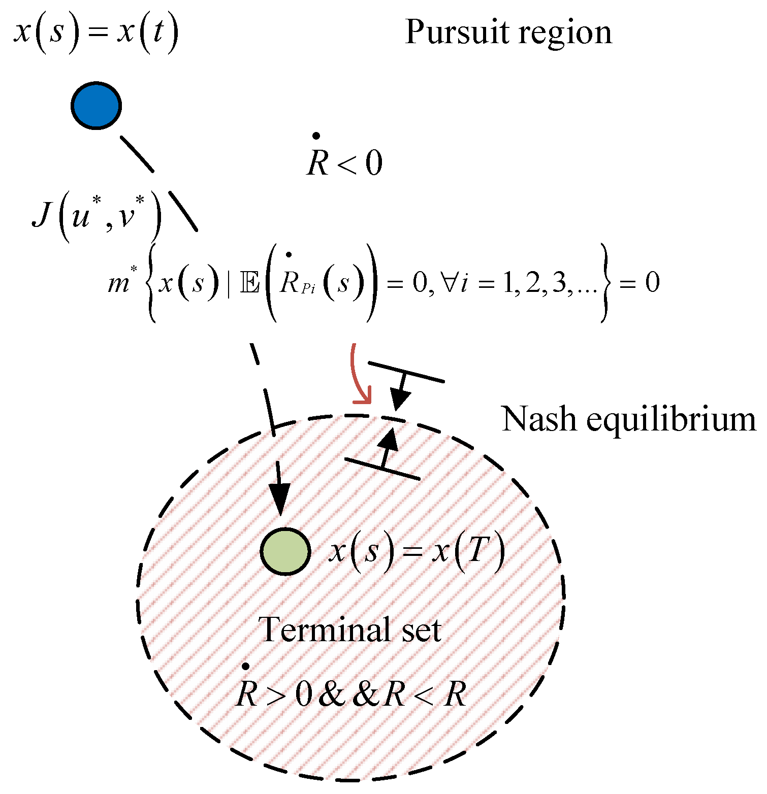
4. The Barrier Surface in the Stochastic Differential Game

Theorem 2. 
The solution x s , t s T of the system (8) under the optimal strategies (77) of the pursuers and evader is globally stable in the sense that for any initial state x 0 , the following holds:
lim sup T 1 T E t T x s 2 d s <
Proof. 
It can be assumed that b s , x s Φ s x s + γ [ t ] v t v [ t ] , where Φ s is uniformly stable and converging to a random matrix Φ , and Φ T ( s ) K ( s ) + K ( s ) Φ ( s ) = I . To facilitate estimation, we employ reduced excitation or exploration signals. We use a random sequence where lim k γ k = 0 , with min γ k k 1 5 and γ 0 = 0 . An independent standard Wiener process sequence is selected to counteract the randomness of the states. It satisfies the following:
lim sup N 1 N k = 1 N k k + 1 γ k 2 v t v k 2 d t = 0 .
System (8) can now be rewritten as follows:
d x ( s ) Φ ( s ) x ( s ) + γ [ t ] ( v ( t ) v ( [ t ] ) ) + b u 1 ( x ( s ) ) u 1 ( s ) + b u 2 ( x ( s ) ) u 2 ( s ) + b v 1 ( x ( s ) ) v 1 ( s ) + b v 2 ( x ( s ) ) v 2 ( s ) d s + σ ( s , x ( s ) , u 1 ( s ) , u 2 ( s ) , v 1 ( s ) , v 2 ( s ) ) d W ( s )
Let Ω = b u 1 b u 2 b v 1 b v 2 T , Σ = u 1 u 2 v 1 v 2 T . The following could be obtained:
d x s Φ s x s + γ t v t v t + Ω T Σ d s + σ d W s
According to the closed optimal backward strategy (77), we could obtain the following:
u 1 = L u 1 x + c u 1 , u 2 = L u 2 x + c u 2 , v 1 = L v 1 x + c v 1 , v 2 = L v 2 x + c v 2 , Σ = L u v x + c u v .
By applying the I t o ^ Lemma, the following can be obtained:
d K ( s ) x ( s ) , x ( s ) = 2 K ( s ) x ( s ) , Φ ( s ) x ( s ) + Ω T ( L u v x + c u v ) + γ [ t ] ( v ( t ) v ( [ t ] ) ) d t + tr ( K ( s ) σ σ T ) d t + 2 K ( s ) x ( s ) , σ d W ( s ) + 1 m u v | x ( s ) | 2 d t = 2 K ( s ) x ( s ) , Ω T c u v + γ [ t ] ( v ( t ) v ( [ t ] ) ) d t + tr ( K ( s ) σ σ T ) d t + 2 K ( s ) x ( s ) , σ d W ( s )
where t T K s x s , σ d W s = O t T x s 2 d t 1 2 + ε , ε 0 , 1 / 2 . By integrating Equation (86) and applying the Cauchy–Schwarz inequality, we obtain the following:
i = t T K ( i 1 ) x ( i ) , x ( i ) K ( i 1 ) x ( i 1 ) , x ( i 1 ) + K ( [ T ] ) x ( T ) , x ( T ) K ( [ T ] ) x ( [ T ] ) , x ( [ T ] ) + K ( [ t ] ) x ( t ) , x ( t ) K ( [ t ] ) x ( [ t ] ) , x ( [ t ] ) + t T 1 m u v | x ( t ) | 2 d t = t T 2 K ( s ) x ( s ) , Ω T c u v + γ [ t ] v ( t ) v ( [ t ] ) d t + t T tr K ( s ) σ σ T d t + t T 2 K ( s ) x ( s ) , σ d W ( s ) = O t T | x ( s ) | 2 d t 1 2 + O t T | x ( s ) | 2 d t t T γ [ t ] 2 v ( t ) v ( [ t ] ) 2 d t 1 2 + O ( T ) + O t T | x ( s ) | 2 d t 1 2 + ε
Then, according to Equation (87), and integrating the system Equation (83), the integral interval is k , k + 1 .
x k + 1 e Φ k x k + k k + 1 e k + 1 s Φ k γ t v s v k + Ω T c u v d s + k k + 1 e k + 1 s Φ k σ d W s
According to the Cauchy–Schwarz inequality, the following can be concluded:
x k + 1 2 m x k 2 + m 2 k k + 1 Ω T c u v d s 2 + m 3 k k + 1 γ t v s v k 2 d s + m 1 k k + 1 e k + 1 s Φ k σ d W s 2
where 0 < m < 1 , m 1 , m 2 , m 3 > 0 . Some fixed constants are relative to the maximum of e Φ k , k N .
k = 1 N x k 2 m k = 0 N 1 x k 2 + m 2 0 N 1 Ω T c u v 2 d s + m 3 i = 0 N 1 k k + 1 γ k 2 v s v k 2 d s + m 1 k = 0 N 1 k k + 1 e k + 1 s Φ k σ d W s 2 .
The following could be obtained:
lim N 1 m N k = 1 N x k 2 m N x 0 2 + m 2 N 0 N 1 Ω T c u v 2 d s + m 3 N i = 0 N 1 k k + 1 γ k 2 v s v k 2 d s + m 1 N k = 0 N 1 k k + 1 e k + 1 s Φ k σ d W s 2 .
Since the second term is bounded and the expectation of the third and fourth terms are equal to zero, we obtain the following:
lim sup T E 1 T t T x s 2 d s < .
This shows that for the state variables, as time approaches infinity, the norm of the state is a linear function of time. Hence, the proof is completed. □
Let x i s : Ω i , F i , P i Ω , F , s t , T be two stochastic processes. The processes x 1 s and x 2 s are said to have the same finite-dimensional distribution on t , T if there exists a set D of full measures on t , T , such that for all t t 1 t 2 t n T , where t i D and A F n (with ⊗ denoting the tensor product). We have the following:
P 1 W 1 , x 1 t 1 , x 1 t 2 , , x 1 t n A = P 2 W 2 , x 2 t 1 , x 2 t 2 , , x 2 t n A .
This can be written as L P 1 x 1 = L P 2 x 2 , where L P i denotes the law of the process x i under probability measure P i . Now, let μ 1 = Ω 1 , F 1 , F s 1 , t , P 1 , W 1 and μ 2 = Ω 2 , F 2 , F s 2 , t , P 2 , W 2 be two filtered probability spaces.
Theorem 3. 
Let η i L 2 Ω i , F s i , t , P i , and let x i ( s ) be the unique solution of the state equation given the control inputs u 1 i , u 2 i U , v 1 i , v 2 i ν with initial state x i ( t ) = η t . If the following equality holds:
L P 1 u 1 1 , u 2 1 , v 1 1 , v 2 1 , W 1 , η 1 = L P 2 u 1 2 , u 2 2 , v 1 2 , v 2 2 , W 2 , η 2
then we have:
L P 1 x 1 , u 1 1 , u 2 1 , v 1 1 , v 2 1 = L P 2 x 2 , u 1 2 , u 2 2 , v 1 2 , v 2 2
Proof. 
x i s are the obtained limits of iterations of the maps. This implies the following:
K i z i s = η t + t s B r , z i r , u 1 i , u 2 i , v 1 i , v 2 i d r + t s σ r , z i r , u 1 i , u 2 i , v 1 i , v 2 i d W
where z 1 i s = η i , z k + 1 i s = K i z k i s , x i s = lim k z k + 1 i s .
z k 1 s z k 2 s = t s B r , z k 1 1 r , u 1 1 , u 2 1 , v 1 1 , v 2 1 B r , z k 1 2 r , , u 1 2 , u 2 2 , v 1 2 , v 2 2 d r + t s σ r , z k 1 1 r , u 1 1 , u 2 1 , v 1 1 , v 2 1 σ r , z k 1 2 r , u 1 2 , u 2 2 , v 1 2 , v 2 2 d W
Hence, we use the Burkholder–Davis–Gundy inequalities in the first term and writing C z for the constant in the inequalities.
E z k 1 s z k 2 s 2 2 E t s B r , z k 1 1 r , u 1 1 , u 2 1 , v 1 1 , v 2 1 B r , z k 1 1 r , , u 1 1 , u 2 1 , v 1 1 , v 2 1 d r 2 + t s σ r , z k 1 2 r , u 1 2 , u 2 2 , v 1 2 , v 2 2 σ r , z k 1 2 r , u 1 2 , u 2 2 , v 1 2 , v 2 2 d W 2 2 C z E t s σ r , z k 1 1 r , u 1 1 , u 2 1 , v 1 1 , v 2 1 σ r , z k 1 1 r , u 1 1 , u 2 1 , v 1 1 , v 2 1 2 d W + T E t s B r , z k 1 2 r , u 1 2 , u 2 2 , v 1 2 , v 2 2 B r , z k 1 2 r , , u 1 2 , u 2 2 , v 1 2 , v 2 2 2 d r 2 C z + T C k 2 E t s z k 1 1 z k 1 2 2 d r C v E t s z k 1 1 z k 1 2 2 d r
where C v = 2 C z + T C k 2 . According to this definition, we could have the following:
L P 1 z k 1 , w 1 , u 1 1 , u 2 1 , v 1 1 , v 2 1 = L P 2 z k 2 , w 2 , u 1 2 , u 2 2 , v 1 2 , v 2 2 .
This implies the following:
E x 1 s x 2 s 2 = lim k E z k 1 s z k 2 s 2 lim k C v 1 E t s z k 1 1 z k 1 2 2 d r . . . lim k C v n E t s z 1 1 z 1 2 2 d r C v E t s η t η t 2 d r 0 .
Therefore, passing to the limit as k gives the following result: E x 1 s = E x 2 s . This completes the proof. □
Theorem 4. 
According to Assumptions 1 and 2, there exists a unique solution for ( s , x , α , u 1 * , u 2 * , v 1 * , v 2 * ) [ t , T ] × R m × 1 × R m × m × R n × 1 × R n × 1 × R 1 × 1 × R 1 × 1 to the forward–backward stochastic differential equations (FBSDEs).
Proof. 
(The proof by contradiction): Suppose that there exist two solutions, x 1 , α 1 , u 1 1 , u 2 1 , v 1 1 , v 2 1 , x 2 , α 2 , u 1 2 , u 2 2 , v 1 2 , v 2 2 , and denote x ^ = x 1 x 2 , α ^ = α 1 α 2 , u ^ 1 = u 1 1 u 1 2 , u ^ 2 = u 2 1 u 2 2 , v ^ 1 = v 1 1 v 1 2 . Then, we can obtain the following:
d x ^ s = b + b u 1 u ^ 1 s + b u 2 u ^ 2 s + b v 1 v ^ 1 s + b v 2 v ^ 2 s d s , + σ ^ d W s , d p ^ = α ^ d s + β ^ d W = A T p ^ + ζ x ^ E ( x ^ ) d s + β ^ d W , x ^ 0 = 0 , p ^ T = R T x ^ T E x ^ T .
Applying the I t o ^ Lemma to p ^ , x ^ and taking the expectation on both sides:
0 = E R T x ^ T E ( x ^ T ) , x ^ + E p ^ , d x ^ + E d p ^ , x ^ + E d p ^ , d x ^ = E R T x ^ T E ( x ^ T ) , x ^ + E p ^ , b + b u 1 u ^ 1 ( s ) + b u 2 u ^ 2 ( s ) + b v 1 v ^ 1 ( s ) + b v 2 v ^ 2 ( s ) d s + σ ^ d W + E A T p ^ + ζ x ^ E ( x ^ ) d s + β ^ d W , x ^ + E β T σ d s = E R T x ^ T E ( x ^ T ) , x ^ T + E ( t T ( p ^ T b + b u 1 u ^ 1 ( s ) + b u 2 u ^ 2 ( s ) + b v 1 v ^ 1 ( s ) + b v 2 v ^ 2 ( s ) + x ^ T A T p ^ + ζ x ^ E ( x ^ ) + β T σ ) d s ) E R T 1 2 x ^ T E ( x ^ T ) , R T 1 2 x ^ T E ( x ^ T ) + E t T ζ 1 2 x ^ E ( x ^ ) , ζ 1 2 x ^ E ( x ^ ) d s .
Thus, we obtain E x ^ T E x ^ T = 0 , and E ζ x ^ E x ^ = 0 , which implies that p ^ 0 . Therefore, the value function is the unique viscosity solution of the HJB equation, indicating that S 1 , S 2 , S 3 , S 4 are unique. Consequently, we have E u ^ 1 ( s ) = E u ^ 2 ( s ) = E v ^ 1 ( s ) = E v ^ 2 ( s ) . This leads to E x ^ = 0 . This completes the proof. □
Based on the global stability and uniqueness of the state, we can derive a comprehensive mapping of state information relative to the initial conditions. Next, we will explore the Lebesgue measure problem associated with barrier surfaces in the context of Nash equilibrium.
Theorem 5. 
The Lebesgue measure of a set composed of state points where the distance change rate between pursuers and evaders (Nash equilibrium) is zero is shown in Figure 5:
m * x s | E R P i s = 0 , i = 1 , 2 , 3 , . . . = 0
Proof. 
The barrier surface can be defined as the set of points where the relative dynamics between the evader and pursuer reach a critical state such that the expected relative velocity projection between the two becomes zero. Mathematically, this surface is expressed as follows:
I i = x ( s ) | E R P i s = 0 , i = 1 , 2 , 3 , ,
where
R P i = v E cos θ E cos φ E v P i cos θ P i cos φ P i ,
with I i = ( θ E , φ E , θ P i , φ P i ) representing the points on the barrier surface such that
v E cos θ E cos φ E = v P i cos θ P i cos φ P i .
The barrier surface describes the critical configurations where the pursuer’s control actions cannot effectively reduce the distance to the evader. This implies that the states on the barrier surface act as a dynamic boundary between regions of successful pursuit and regions where the evader can potentially avoid capture. The barrier surface can be further understood as a countable set of points:
I n = I 1 , I 2 , , I N , ,
with a small neighborhood around each point:
Q ξ = Q 1 , Q 2 , Q 3 , , Q N , , Q i = B I i , ε N I i ,
where I i I n . According to the nested open interval theorem, there exists ε > 0 such that the neighborhoods Q ξ form a cover for the points on the barrier surface. The measure of these points on the barrier surface can be expressed as follows:
m * I n = i = 1 m * I i = inf m * Q ξ = inf m * i = 1 Q i
Thus:
inf m * i = 1 Q i inf i = 1 N m Q i 4 3 π ε 3 N 3 N ( 1 + N ) 2 2 3 π ε 3 N
where m * Q i = 4 3 π ε N 3 represents the volume of the ball. This implies the following:
m * I n 2 3 π ε 3 N .
Taking the limit as ε 0 , we obtain the following:
lim ε 0 m * I n lim ε 0 2 3 π ε 3 N 0
where N is a real number with an upper bound. Thus, m * ( I n ) = 0 , completing the proof. □
Note: In the context of stochastic differential games, the Lebesgue measure of the barrier surface is zero, which divides the state space of the pursuit region into two distinct parts: the pursuit region and the terminal region. The state within the pursuit region has two ranges, and there is no equilibrium state between the pursuer and the evader. When discussing the equilibrium problem, it is important to clarify that equilibrium is not the desired outcome. We are primarily concerned with two results: capture and escape. Once an equilibrium state is reached, it indicates that the current strategies are ineffective—neither allowing the pursuer to capture the evader nor enabling the evader to escape from the pursuit region. Even if a termination time is established, the final state cannot be regarded as the definitive outcome of the game. Given any initial conditions, the state trajectory over a certain time frame is unique. Notably, when the state transitions through the barrier surface from the pursuit region to the terminal region, the time required for this transition is effectively zero.
In practical pursuit scenarios, it is often assumed that both sides maintain a balanced state when evenly matched. However, in reality, this balance is not static but fluctuates around the equilibrium. Using a missile interception model as our simulation framework, we illustrate that the condition R ˙ = 0 , representing a constant relative distance, does not persist in real-world scenarios. Instead, interception success corresponds to R ˙ < 0 , while R ˙ > 0 indicates that the evader escapes, resulting in the two participants diverging. This highlights an important insight: the condition R ˙ = 0 is a transient state, consisting of a set of discrete points forming a surface with a Lebesgue measure of zero. In practical terms, this means that the system’s state crosses the barrier surface in zero time. For missile interception problems, this translates to a binary outcome—either interception is successful, or it fails entirely.

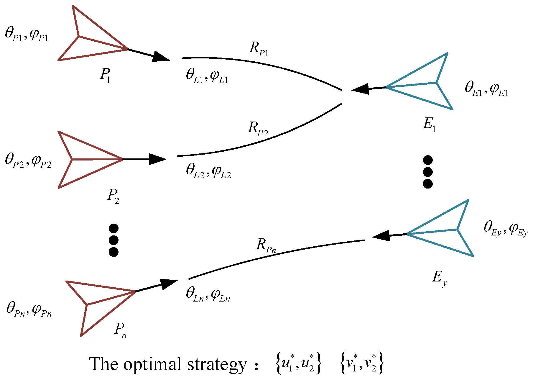
5. The Multiple Pursuers and Evaders in a Stochastic Differential Game

When multiple pursuers are chasing evaders, the pursuers should be grouped, then each group should be incorporated into the state equation. As shown in Figure 6, the pursuit process is divided into the following five steps:
  • Step 1: Dividing the n pursuers into groups, with each group corresponding to a respective number of evaders denoted by y.
  • Step 2: Substituting the information of the pursuers into the system Equation (8), where v 1 ( s ) R y × 1 and v 2 ( s ) R y × 1 . The status includes the following: Status : { R P 1 , R P 2 , , θ L 1 , φ L 1 , θ L 2 , φ L 2 , , θ P 1 , φ P 1 , θ P 2 , φ P 2 , , θ E 1 , φ E 1 , θ E 2 , φ E 2 , } .
  • Step 3: Calculating the parameters S 1 , S 2 , S 3 , S 4 of the value function based on the H J B equation.
  • Step 4: Solving for the optimal closed-loop feedback strategies u 1 * , u 2 * , v 1 * , v 2 * based on FBSDEs.
  • Step 5: Implementing the optimal strategies into the motion equations for the pursuers to capture the evaders.

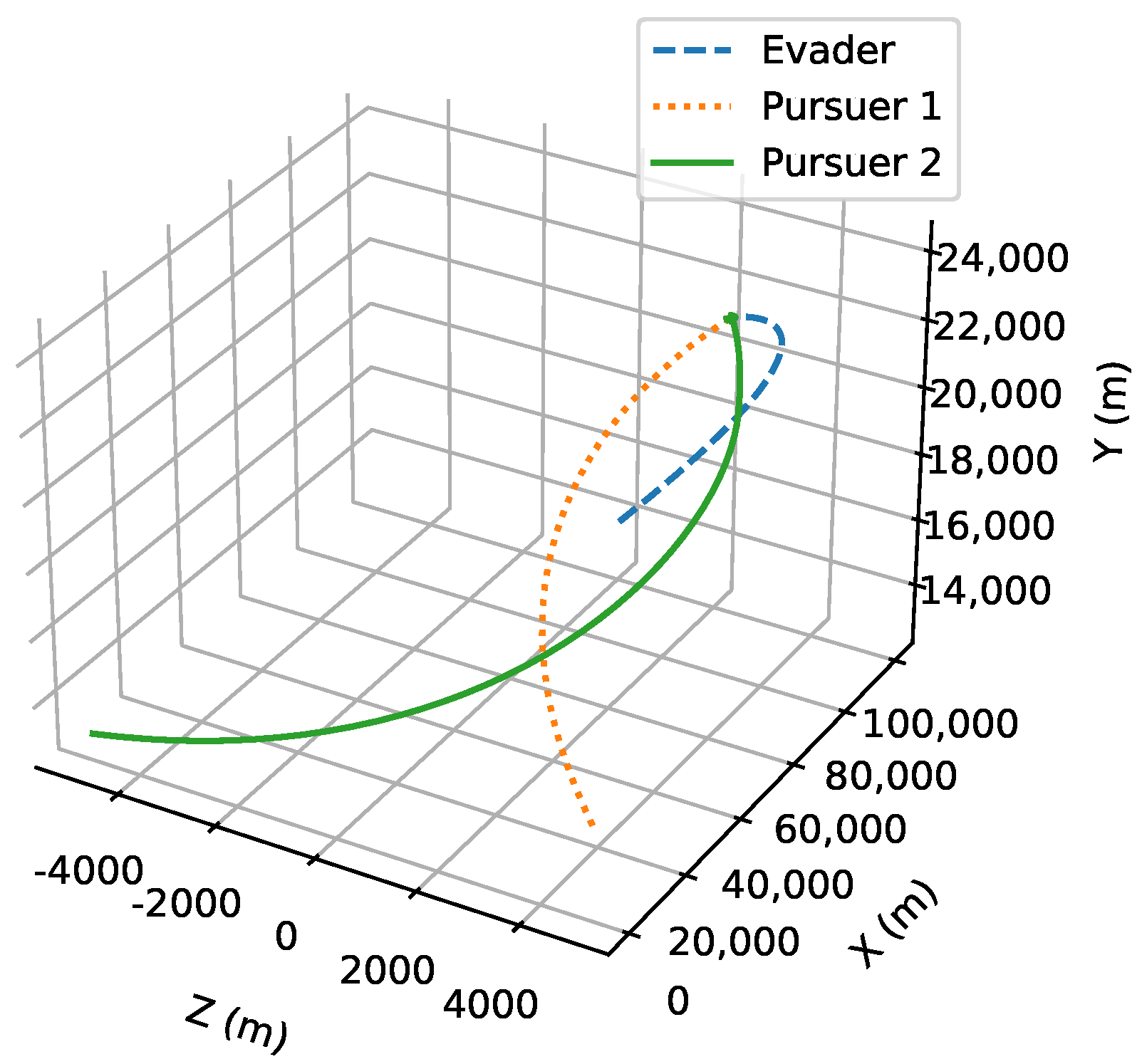
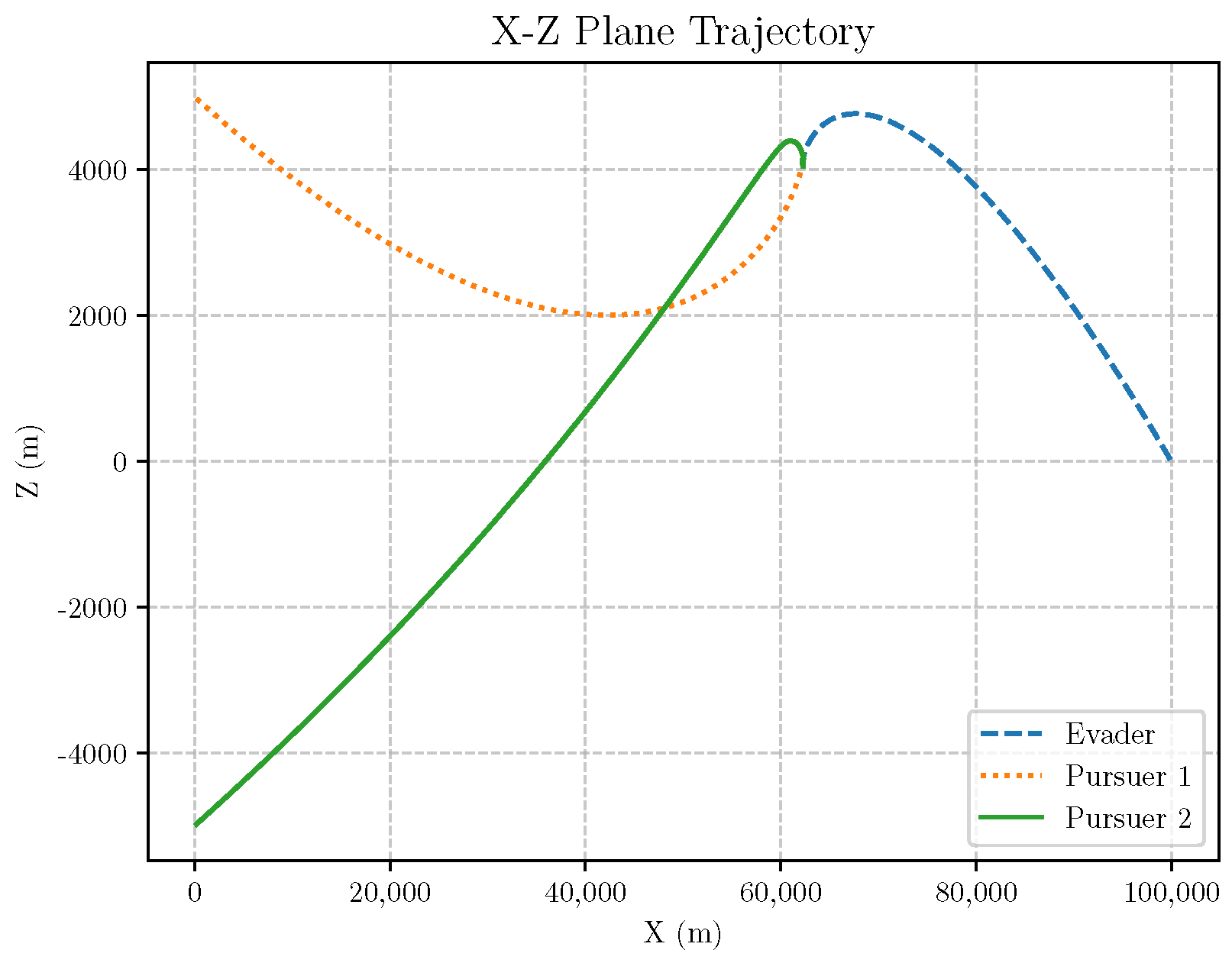
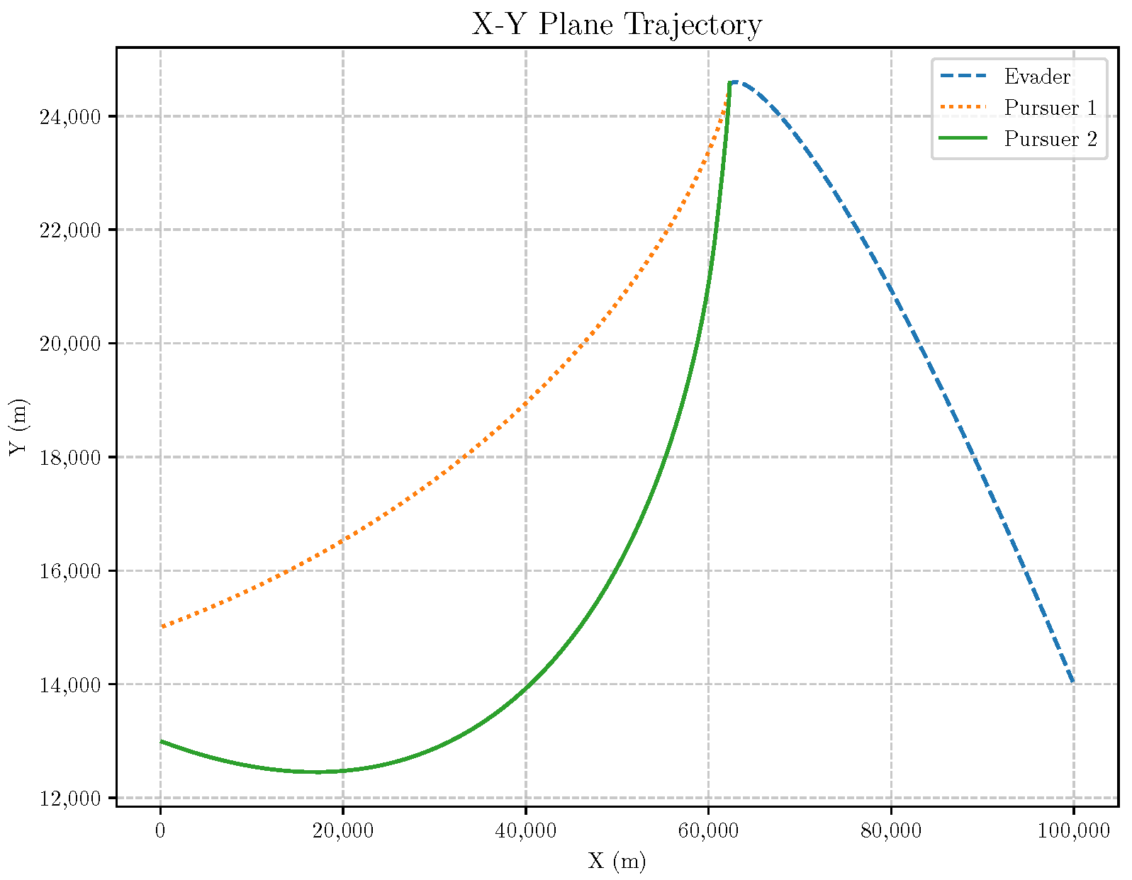
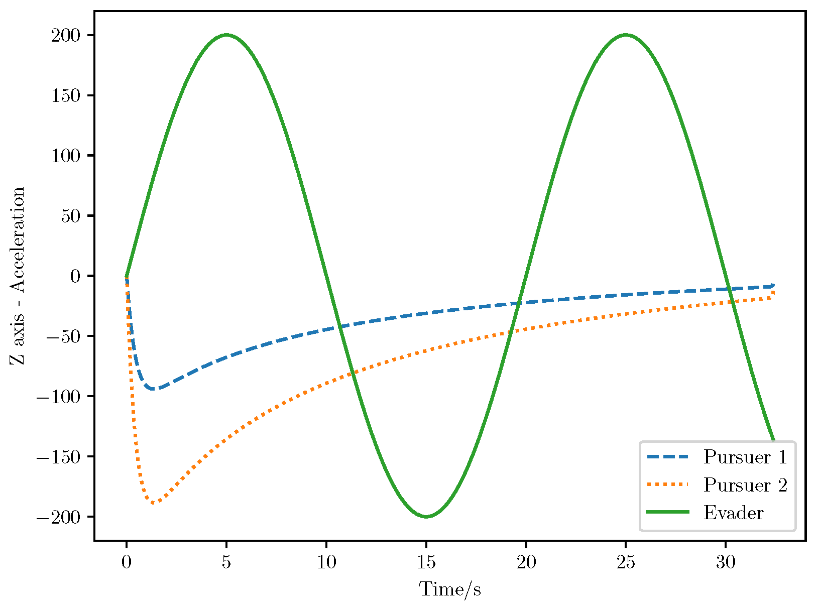
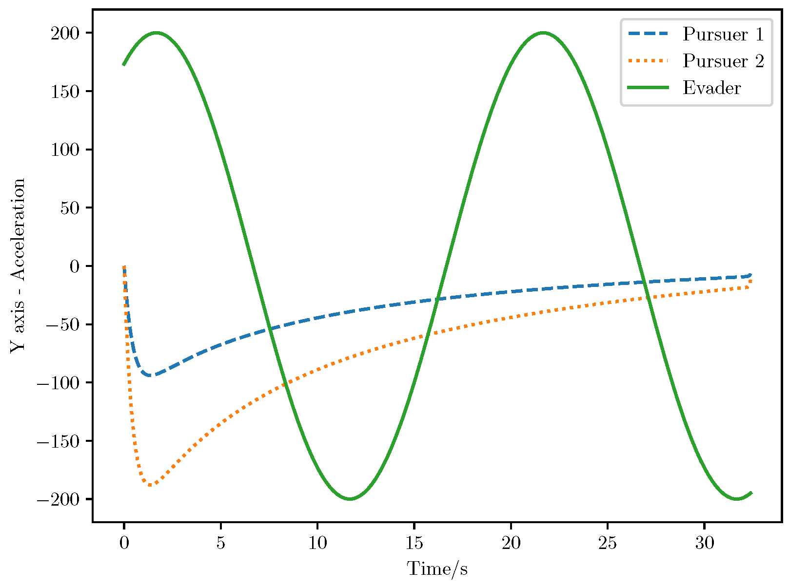
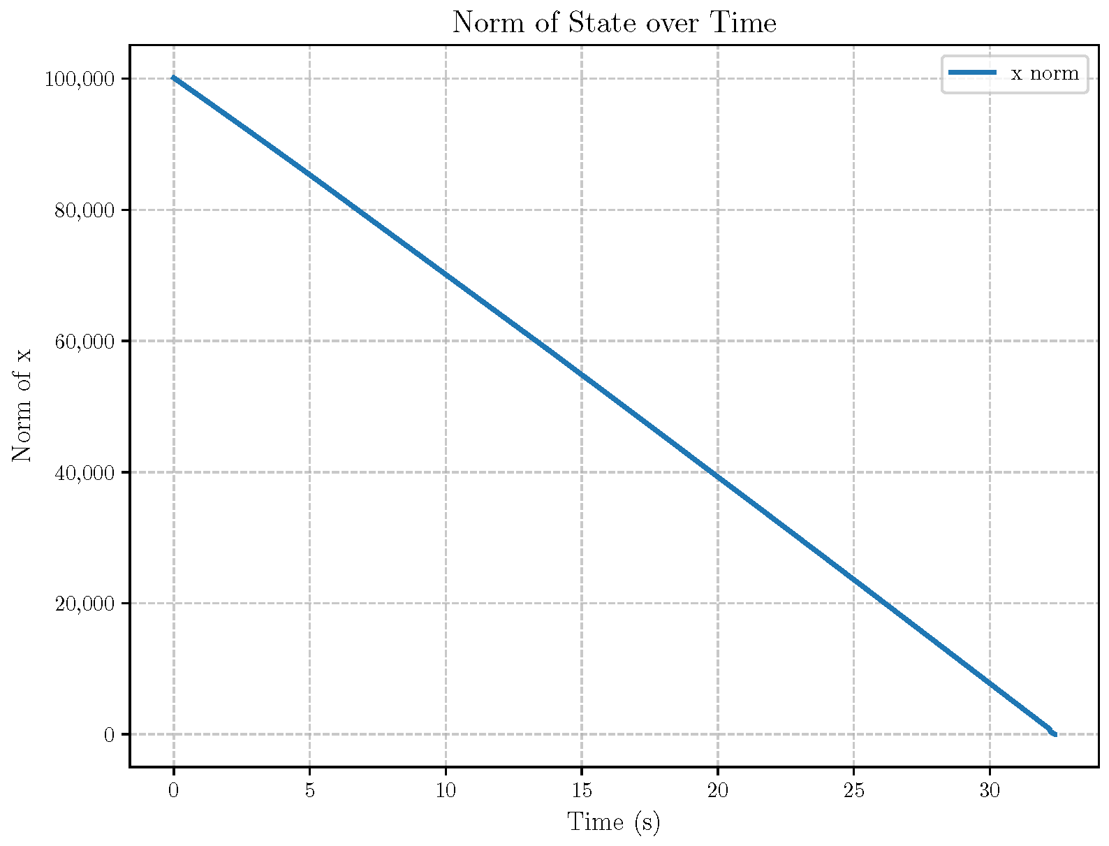
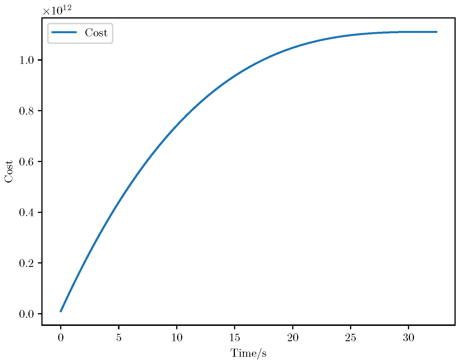
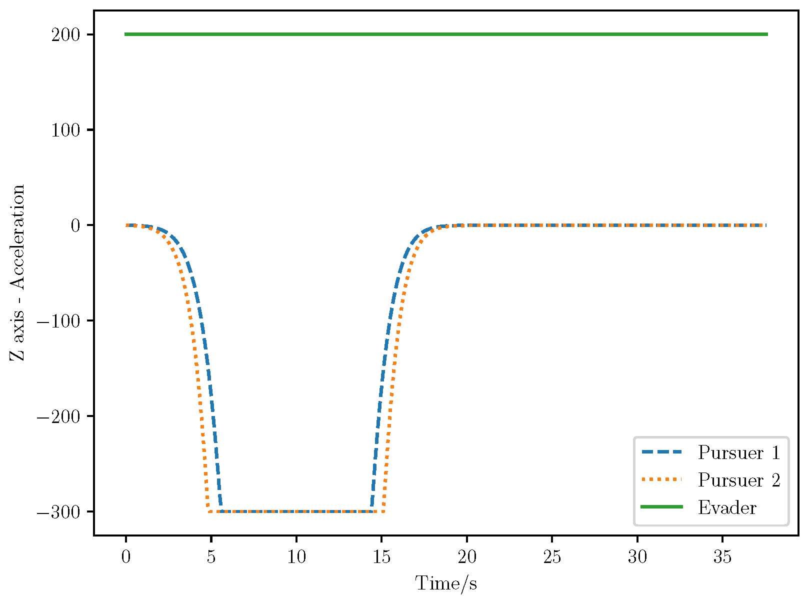
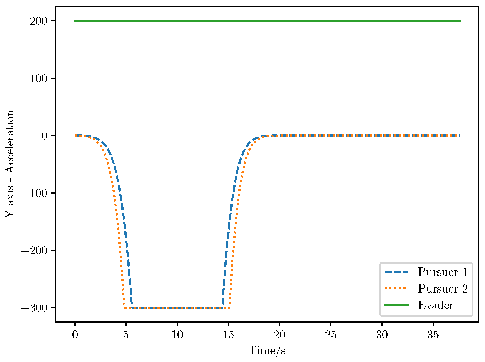
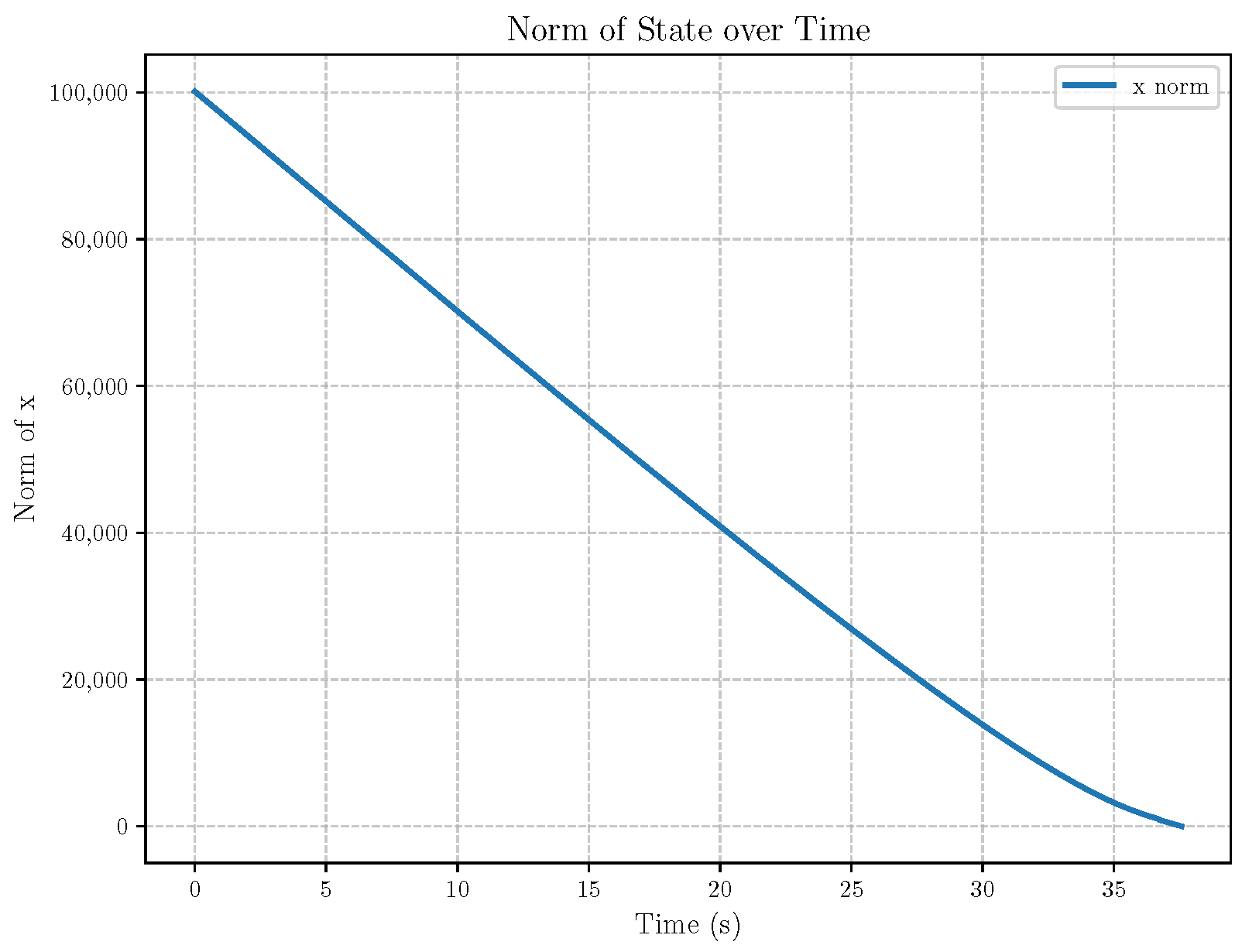
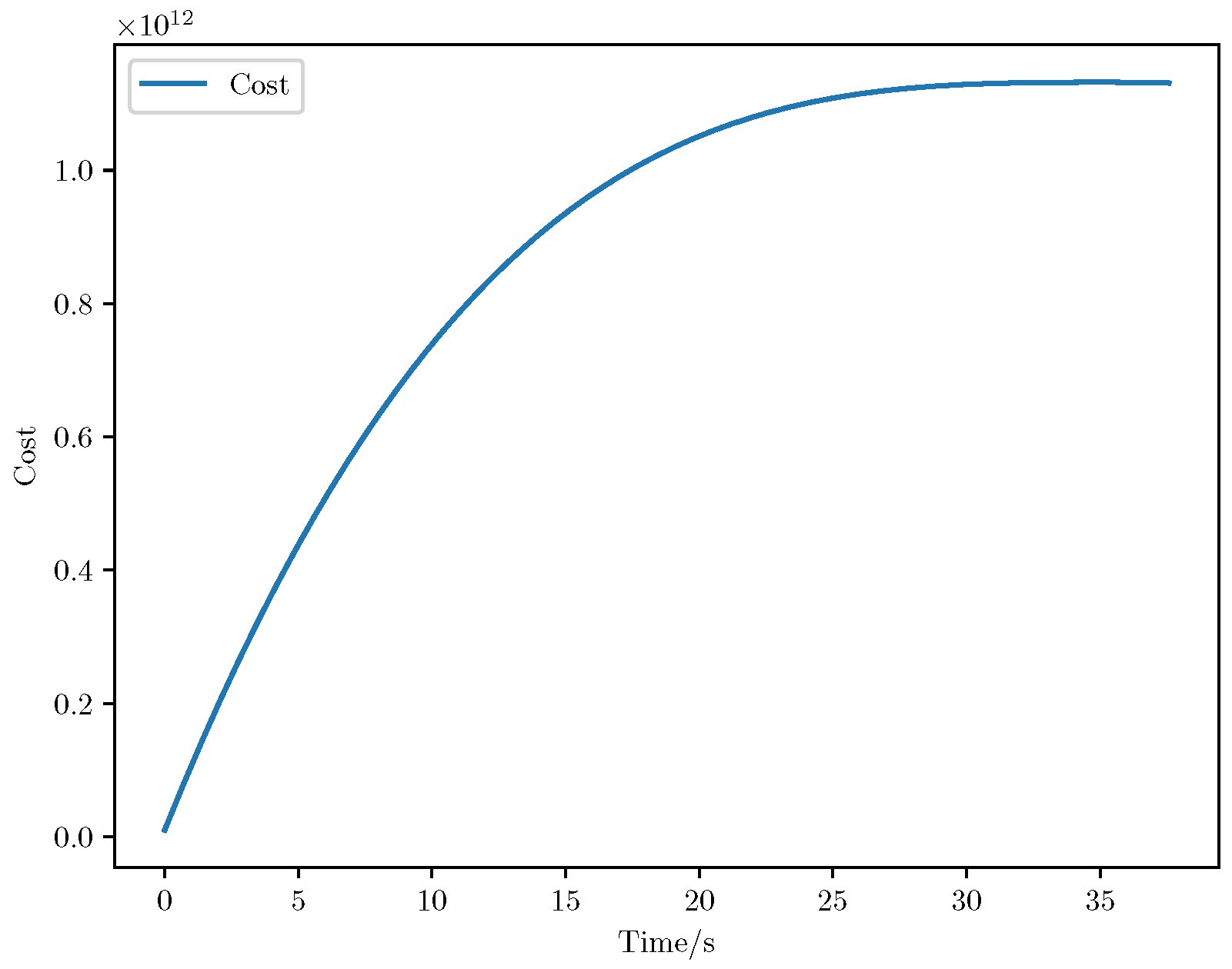
6. Numerical Analysis

Example 1. 
The initial conditions for this simulation are as follows:
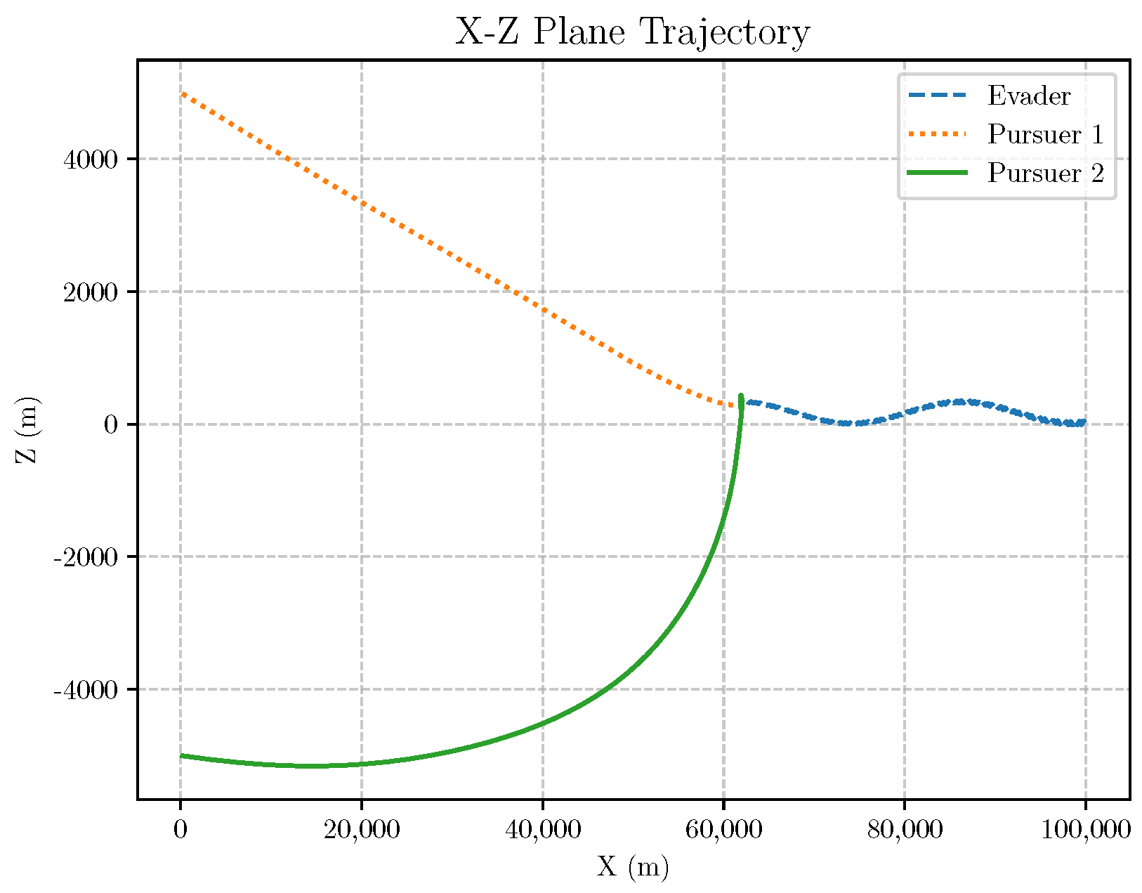
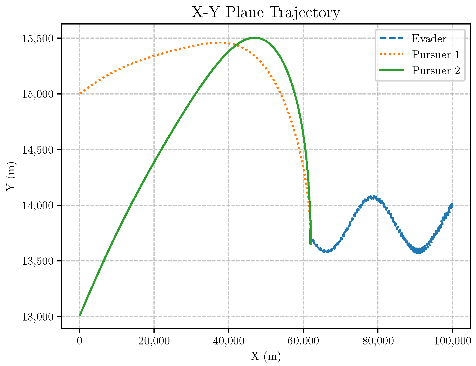
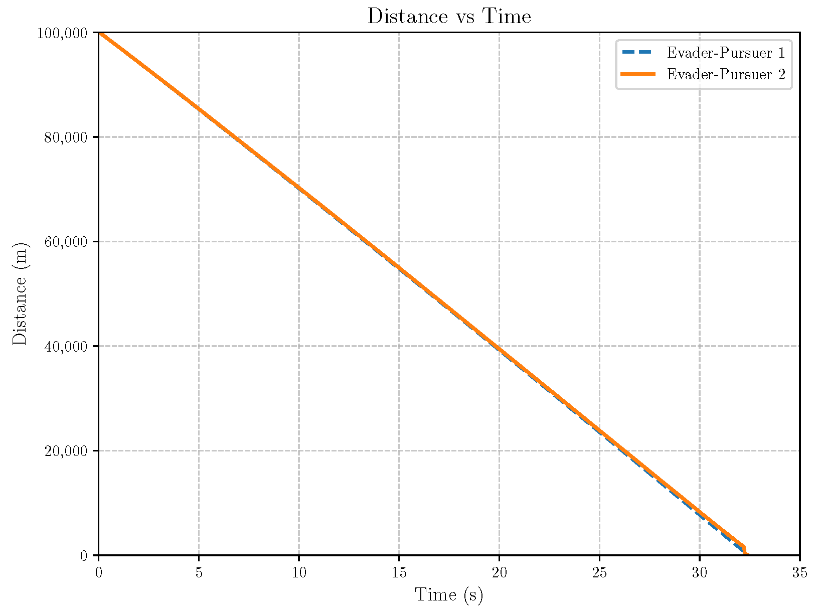
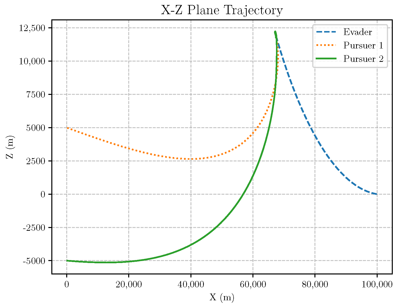
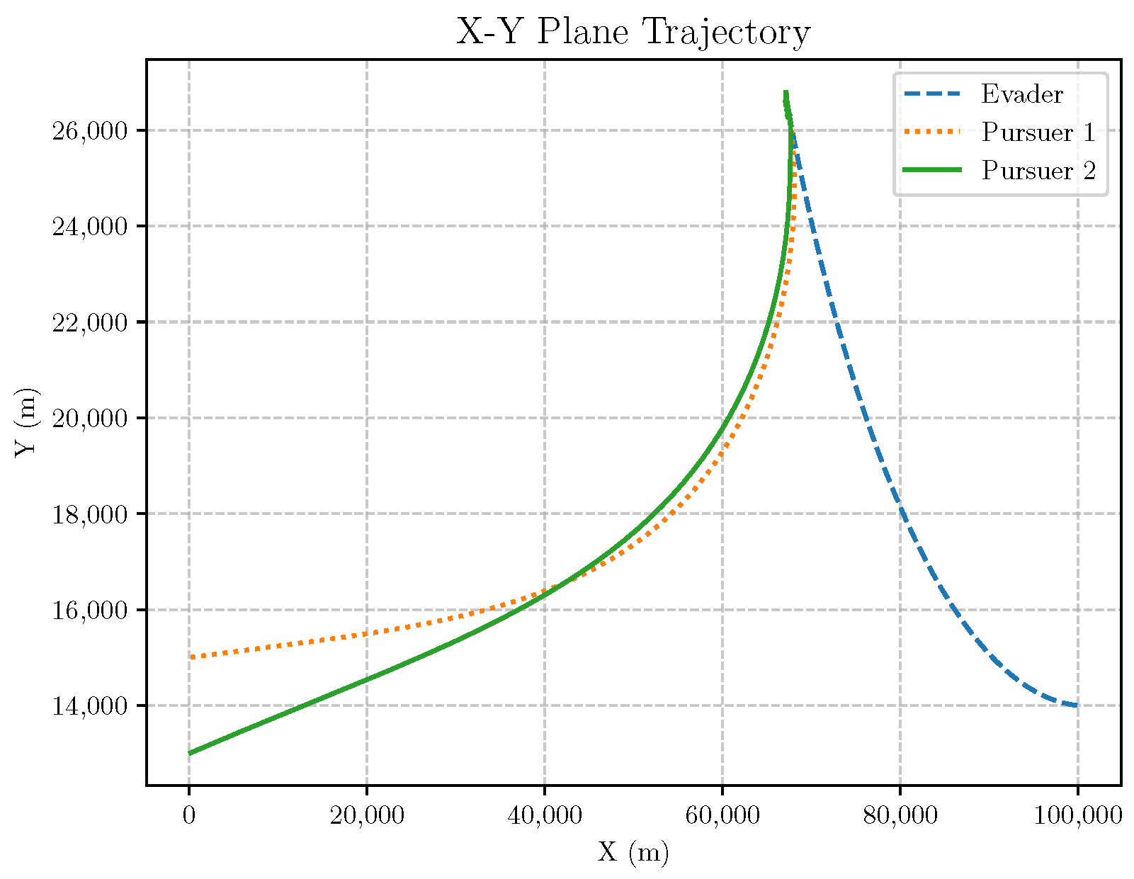
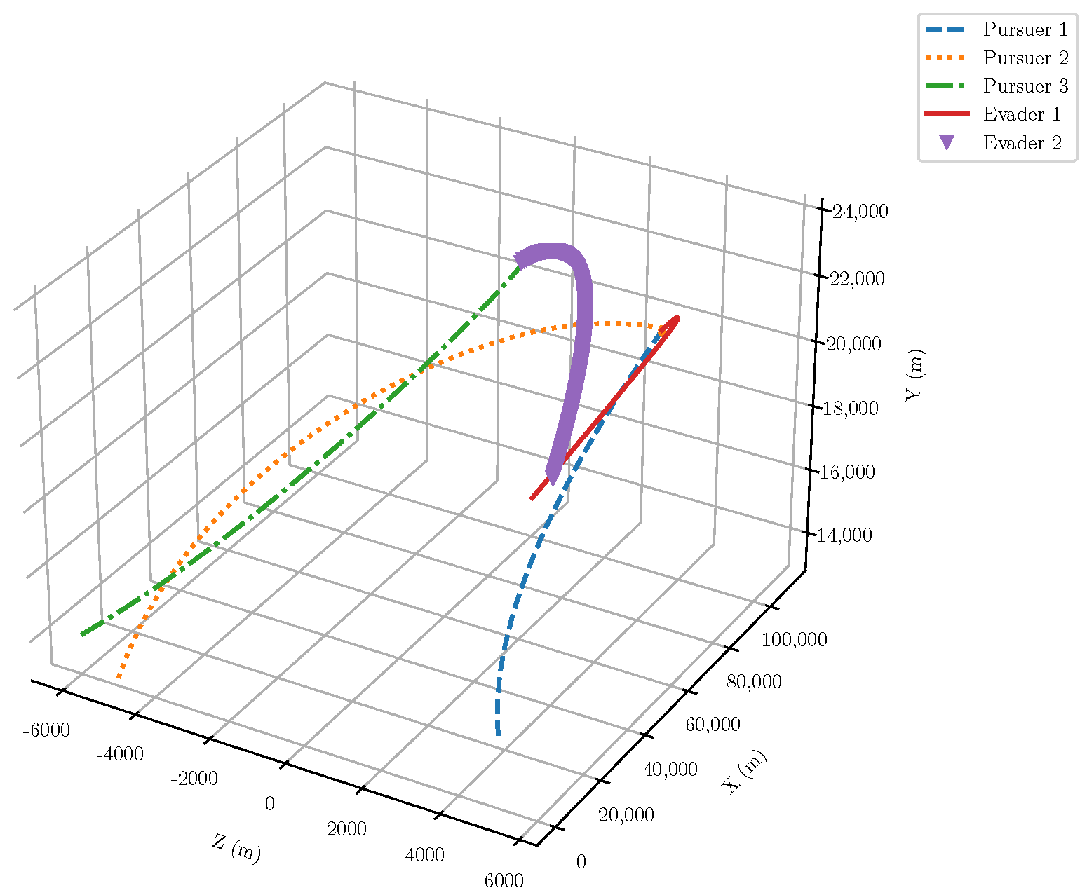
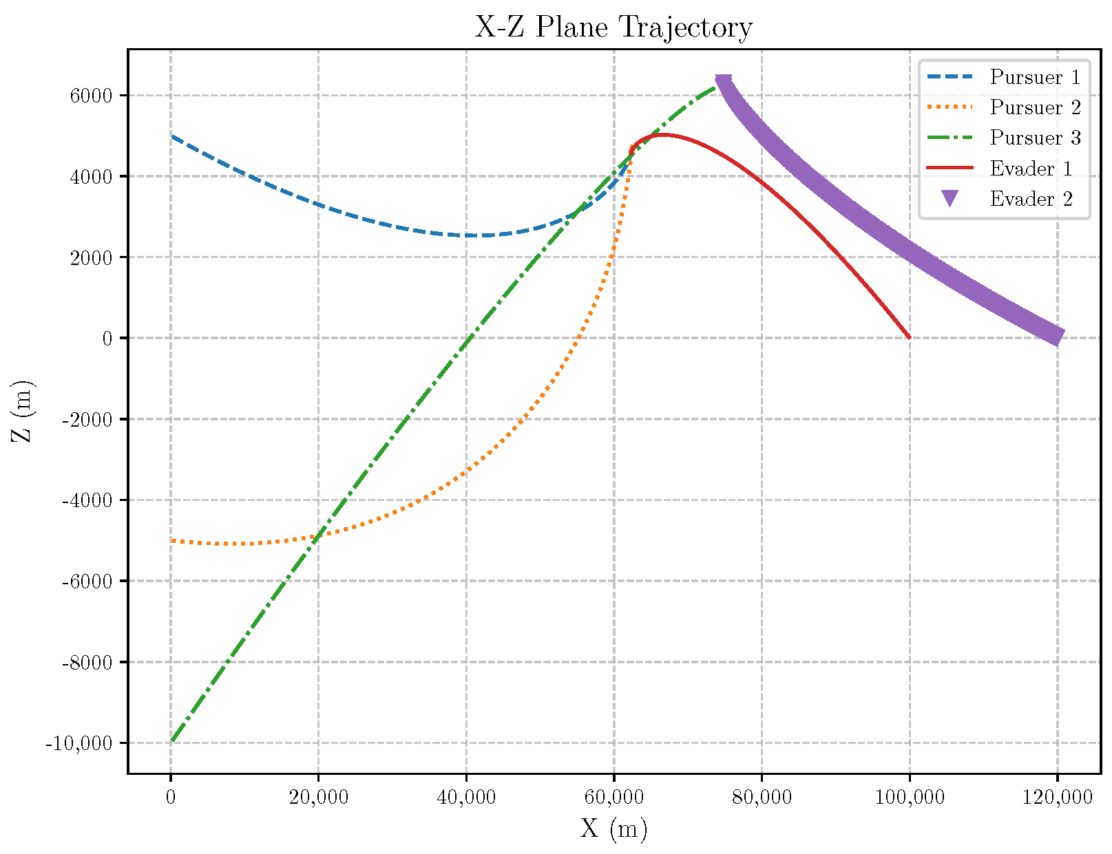
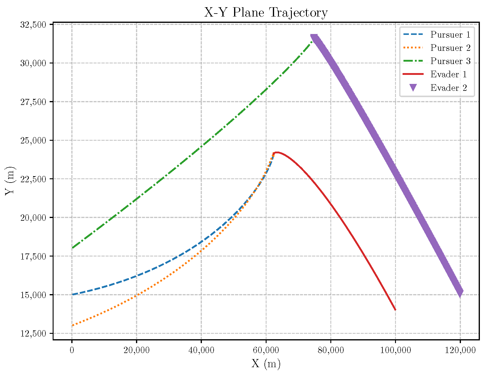
  • Initial positions: The initial position of pursuer P 1 is [0, 15,000, 5000] m, while that of P 2 is [0, 13,000, −5000] m. The initial position of the evader E is [100,000, 14,000, 0] m.
  • Initial velocities: The pursuers’ velocities are set to 3000 m/s and 3500 m/s, respectively, while the evader’s velocity is 2000 m/s.
  • Acceleration limits: The maximum normal accelerations are 30 g for the pursuers and 20 g for the evader (g = 9.81 m/s2).
  • Flight path angles: The initial flight path angles for the pursuers are set to −4° (elevation) and 4° (azimuth). The evader’s initial angles are 10° (elevation) and 170° (azimuth).
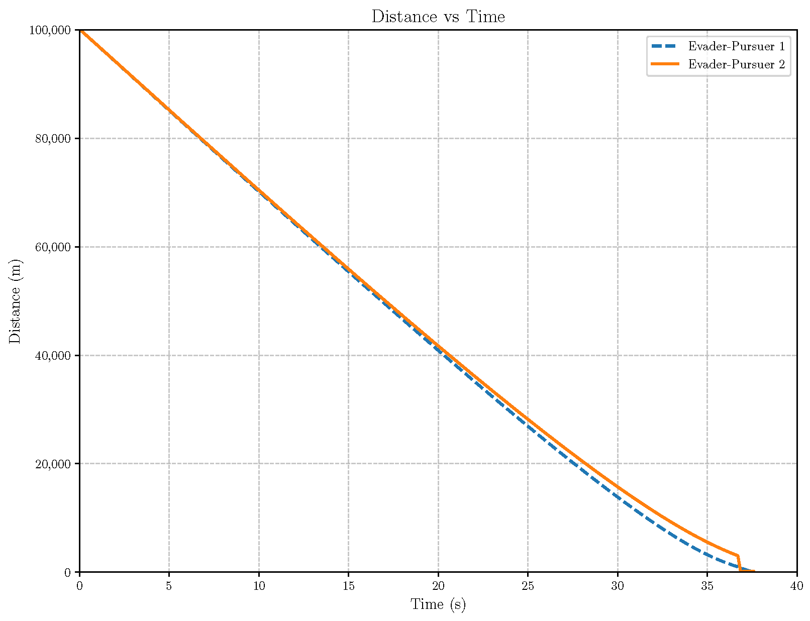
  • Time step: A time interval of 0.1s was used for numerical integration.
During the simulation, both the pursuers and the evader employ the optimal strategy. The optimal trajectory is depicted in Figure 7. Two-dimensional projections in the X–Y and X–Z planes are shown in Figure 8 and Figure 9, respectively. These figures demonstrate the feasibility of the optimal state feedback strategy algorithm proposed in this paper. The distance between the evader and the pursuers is illustrated in Figure 10, where the final miss distance is 0.83 m . In missile interception problems, it is commonly assumed that interception occurs when the distance is less than one meter. Furthermore, in this paper, the interception termination set is defined by R ˙ > 0 or R < 1 . The evader is captured by the pursuers after 31.7 s . Generally, the terminal guidance phase of missile interception lasts between 20 s and 40 s, and the result from Experiment 1 is within this range. Acceleration variations are presented in Figure 11 and Figure 12. The state norm is shown in Figure 13. During the interception process, the state continuously converges, and we have proven this in Theorem 2. The experimental results confirm the validity of Theorem 2, with the terminal state approaching zero. The value of the cost function is shown in Figure 14. It is evident that the cost function converges to a constant value, indicating the convergence of state and input over a finite time. The value function is shown in Figure 15. The value function satisfies the termination condition of the forward–backward stochastic differential equation, with the terminal value being zero. The simulation environment is summarized in Table 2. During the simulation process, the Runge–Kutta method is utilized for each iteration.
The mean value of the state is 503,775.07. The state graph demonstrates that the state norm gradually converges as time increases, indicating that as the time approaches the termination point, the state norm behaves like a linear function. Concurrently, the cost function stabilizes at a constant value, showing a decreasing growth rate over time. Furthermore, the value function satisfies the final convergence criterion, with V ( T ) = 0 .
Example 2. 
In this case, compared to Example 1, the evader employs a sinusoidal maneuver while the pursuer utilizes an optimal feedback strategy, with all other initial conditions remaining unchanged. After 32 s, the pursuer successfully captures the evader, achieving a mission distance of 0.38 m. The mean state value is 504,990.71. The three-dimensional pursuit diagram is displayed in Figure 16, while two-dimensional plane projections in the X–Y and X–Z planes are shown in Figure 17 and Figure 18, respectively. Since the evader’s maneuver is different from that in Example 1, the optimal trajectory is also different. However, in both cases, the pursuer successfully intercepts the evader. The primary objective of Example 2 is to demonstrate that, even when the evader adopts different evasion maneuvers, the pursuer is still able to intercept the evader. The distance between the evader and the pursuer is illustrated in Figure 19, confirming that the evader is captured. Acceleration variations are depicted in Figure 20 and Figure 21. The state norm is shown in Figure 22, the cost function in Figure 23, and the value function in Figure 24. The final experimental results confirm the feasibility of the proposed algorithm.
Example 3. 
In this scenario, the evader employs a constant maneuver while the pursuer implements an optimal feedback strategy, with all other initial conditions remaining unchanged from Example 1. The pursuer successfully captures the evader, resulting in a final mission distance of 0.62 m. The mean state converges to 460,599.78, and the value function reaches zero at the moment of capture. The three-dimensional pursuit diagram is illustrated in Figure 25. Two-dimensional plane projections in the X–Y and X–Z planes are shown in Figure 26 and Figure 27, respectively. In Experiment 3, since the evader employs a constant-value maneuver, the trajectory of the target in three-dimensional space forms an arc. The distance between the evader and the pursuer is depicted in Figure 28, confirming that the evader has been captured. Additionally, the acceleration variations are presented in Figure 29 and Figure 30. In this experiment, the normal acceleration of the pursuer reached its maximum value, but the pursuer successfully captured the evader. The state norm is shown in Figure 31, the cost function in Figure 32, and the value function in Figure 33. The final experimental results confirm the feasibility of the algorithm.
Based on Examples 1–3, we observe the following: In Example 1, both the pursuers and the evader utilize the optimal feedback strategy, allowing the pursuer to successfully capture the evader. The changes in state throughout the pursuit process align with the proof presented in the theorem, and the cost function converges continuously. Ultimately, the value function approaches the designated terminal value. In Example 2, the evader does not employ the optimal feedback strategy; nevertheless, the pursuer successfully captures the evader in both cases. Notably, the cost function at termination is lower than that observed in Example 1. Furthermore, the data for the value function at the terminal time confirms that V ( T ) = 0 .
Example 4. 
We simulated a scenario involving three pursuers and two evaders. Pursuers 1 and 2 successfully captured Evader 1, while Pursuer 3 captured Evader 2. The final mission distances were recorded as follows: R 2 = 0.91 m and R 3 = 0.75 m . The state ultimately converged to 878,031.05. At the moment of capture, the value function converged to zero. The three-dimensional pursuit diagram is illustrated in Figure 34, while the two-dimensional plane projections in the X–Y and X–Z planes are shown in Figure 35 and Figure 36, respectively. In this experiment, both the pursuers and the evaders employed optimal game strategies. As a result, the pursuers successfully intercepted the evaders. However, due to the change in initial positions, the optimal trajectories differ from those in the previous experiments, demonstrating the adaptability of the strategy to varying initial conditions. The three-dimensional pursuit diagram in Figure 34 clearly shows the distinct paths taken by each pursuer and evader during the pursuit. Figure 37 depicts the distance between the evaders and the pursuers at the moment of capture. The distance between each pursuer and their respective evader decreased progressively over time, confirming the effectiveness of the optimal feedback strategy in achieving interception. The mission distances at the moment of capture were recorded as R 2 = 0.91 m and R 3 = 0.75 m , indicating the close proximity of the pursuers to the evaders when interception occurred. The acceleration variations are presented in Figure 38 and Figure 39. These plots reveal how the pursuers’ accelerations changed throughout the pursuit, with notable spikes occurring during the final stages of interception. These spikes indicate the maximum efforts exerted by the pursuers as they close the gap with the evaders. The state norm is illustrated in Figure 40, showing the progression of the system state during the pursuit. As expected, the state norm decreases steadily, reflecting the convergence of the system towards the interception point. This convergence is a strong indicator of the effectiveness of the optimal strategy. The cost function is shown in Figure 41, and the value function is depicted in Figure 42. The cost function reaches a constant value as the simulation progresses, demonstrating the stability of the optimal strategy. Notably, the value function converges to zero at the moment of capture, indicating that the pursuers successfully achieved their objective of intercepting the evaders. These results confirm the robustness and effectiveness of the optimal game strategy in various pursuit scenarios, as well as the adaptability of the strategy to different initial conditions.
Based on the many-to-many strategy presented in this article, we conducted a simulation for Example 4. The experimental results demonstrated that the pursuer successfully captured the evader, with the state converging to zero and the mean value of the state being finite. At the termination time, the value V ( T ) of the value function equals zero. Both Example 1 and Example 4 illustrate that the proposed many-to-one and many-to-many pursuit algorithms effectively enable the interception of multiple targets. We conducted 100 separate experiments with different initial conditions to test the robustness of the model. The initial positions of the pursuer and evader were randomly selected, with the constraint that the initial distance between them was always greater than 100,000 m. The initial angle was chosen within a predefined permissible range to ensure consistency in all trials. The experimental parameters and results are presented in Table 3. The simulation results indicate a high success rate for interception. Out of the 100 experiments, 98 resulted in successful interception, while only 2 cases saw the evader escaping. This demonstrates that the proposed model and algorithm are highly robust and effective, even under varied initial conditions. Numerical stability: To further assess the stability of the solution, we varied key system parameters such as control input constraints and system dynamics and observed the performance. The results showed that, despite variations in these parameters, the system consistently performed well, with the pursuer successfully intercepting the evader in the majority of the trials. This suggests that the solution to the FBSDEs remains stable and robust, even under small perturbations in the system parameters.

7. Conclusions

In this paper, we investigated optimal backward strategies in pursuit problems through stochastic differential games. We assumed that players’ strategies are bounded, which implies that there are constraints on the actions they can take, ensuring that strategies remain realistic within the context of the game. Our approach emphasizes the uniqueness of the value function as a viscosity solution, providing a robust theoretical foundation for our findings. We demonstrated that the parameters of the optimal backward strategies are intrinsically linked to the solutions of forward–backward stochastic differential equations (FBSDEs) and the terminal conditions of the cost function. This relationship represents a significant extension of the work done in references [10,20], where we offer a matrix formulation of the polynomial growth value function. This formulation not only simplifies the computational aspect of deriving optimal strategies but also enhances the applicability of our findings to real-world scenarios.
Furthermore, we provided the expressions for the optimal strategies through rigorous calculations and established the convergence of the state trajectory within the pursuit region. Our results, illustrated in Figure 6, indicate that when the state transitions from the pursuit region to the termination set, it encounters a barrier surface with a Lebesgue measure of zero. This phenomenon illustrates that the state cannot achieve Nash equilibrium during the pursuit process, reflecting the dynamics observed in actual pursuit scenarios. Finally, we validated our proposed optimal feedback strategy through numerical simulations, which demonstrated effective state convergence and successful evader capture. These findings not only reinforce the theoretical contributions of our work but also open avenues for further research in multi-target pursuit strategies.

Author Contributions

Conceptualization, Y.B. and D.Z.; methodology, Y.B.; software, Y.B.; validation, Y.B., D.Z. and Z.H.; formal analysis, Y.B.; investigation, D.Z.; resources, Z.H.; data curation, Y.B.; writing—original draft preparation, Y.B.; writing—review and editing, D.Z. and Z.H.; visualization, Y.B.; supervision, D.Z.; project administration, D.Z.; funding acquisition, Z.H. All authors have read and agreed to the published version of the manuscript.

Funding

This research was funded by the National Natural Science Foundation of China, grant number 61773142.

Data Availability Statement

No new data were created or analyzed in this study.

Conflicts of Interest

The authors declare no conflicts of interest.

References

  1. Isaacs, R. Differential Games I, II, III, IV; Research Memoranda; RAND Corporation: Santa Monica, CA, USA, 1954. [Google Scholar]
  2. Basar, T.; Olsder, G.J. Dynamic Noncooperative Game Theory, 2nd ed.; SIAM: Philadelphia, PA, USA, 1999. [Google Scholar]
  3. Bagchi, A. Stackelberg Differential Games in Economic Models; Springer: Berlin/Heidelberg, Germany, 1984. [Google Scholar]
  4. Smith, J.M. Evolution and the Theory of Games; Cambridge University Press: Cambridge, UK, 1982. [Google Scholar] [CrossRef]
  5. Yeung, D.W.K.; Petrosyan, L.A. Cooperative Stochastic Differential Games; Springer: New York, NY, USA, 2006. [Google Scholar]
  6. Ho, Y.C.; Bryson, A.; Baron, S. Differential games and optimal pursuit-evasion strategies. IEEE Trans. Autom. Control 1965, 10, 385–389. [Google Scholar] [CrossRef]
  7. Bernhard, P. Linear-quadratic, two-person, zero-sum differential games: Necessary and sufficient conditions. J. Optim. Theory Appl. 1979, 27, 51–69. [Google Scholar] [CrossRef]
  8. Liu, N.; Guo, L. Adaptive Stabilization of Noncooperative Stochastic Differential Games. SIAM J. Control Optim. 2024, 62, 1317–1342. [Google Scholar] [CrossRef]
  9. Engwerds, J.C.; van den Broek, W.A.; Schumacher, J.M. Feedback Nash equilibria in uncertain infinite time horizon differential games. In Proceedings of the 14th International Symposium of Mathematical Theory of Networks and Systems, Perpignan, France, 19–23 June 2000; pp. 1–6. [Google Scholar]
  10. Huang, Q.; Shi, J. Mixed leadership stochastic differential game in feedback information pattern with applications. Automatica 2024, 160, 111425. [Google Scholar] [CrossRef]
  11. Xie, T.H.; Feng, X.W.; Huang, J.H. Mixed linear quadratic stochastic differential leader-follower game with input constraint. Appl. Math. Optim. 2021, 84, S215–S251. [Google Scholar] [CrossRef]
  12. Moon, J. Linear-quadratic stochastic leader-follower differential games for Markov jump-diffusion models. Automatica 2023, 147, 110713. [Google Scholar] [CrossRef]
  13. Lv, S. Two-player zero-sum stochastic differential games with regime switching. Automatica 2020, 114, 108819. [Google Scholar] [CrossRef]
  14. Moon, J. A sufficient condition for linear-quadratic stochastic zero-sum differential games for Markov jump systems. IEEE Trans. Autom. Control 2019, 64, 1619–1626. [Google Scholar] [CrossRef]
  15. Sun, H.; Yan, L.; Li, L. Linear-quadratic stochastic differential games with Markov jumps and multiplicative noise: Infinite-time case. Int. J. Innov. Comput. Appl. 2015, 11, 349–361. [Google Scholar]
  16. Zhang, C.; Li, F. Non-zero sum differential game for stochastic Markovian jump systems with partially unknown transition probabilities. J. Frankl. Inst. 2021, 358, 7528–7558. [Google Scholar] [CrossRef]
  17. Wang, B.; Zhang, H.; Fu, M.; Liang, Y. Decentralized strategies for finite population linear-quadratic-Gaussian games and teams. Automatica 2022, 148, 110789. [Google Scholar] [CrossRef]
  18. Luo, G.; Zhang, H.; He, H.; Jin, Y.; Cui, Y. Mean field theory-based multi-agent adversarial cooperative learning. IEEE Trans. Cybern. 2020, 50, 5052–5065. [Google Scholar]
  19. Bensoussan, A.; Chen, S.K.; Chutani, A.; Sethi, S.P.; Siu, C.C.; Yam, S.C.P. Feedback Stackelberg-Nash equilibria in mixed leadership games with an application to cooperative advertising. SIAM J. Control Optim. 2019, 57, 3413–3444. [Google Scholar] [CrossRef]
  20. Huang, J.; Qiu, Z.; Wang, S.; Wu, Z. Linear quadratic mean-field game-team analysis: A mixed coalition approach. Automatica 2024, 159, 111358. [Google Scholar] [CrossRef]
  21. Liu, N.; Guo, L. Stochastic Adaptive Linear Quadratic Differential Games. IEEE Trans. Autom. Control 2022, 69, 1066–1073. [Google Scholar] [CrossRef]
  22. Hamadène, S. Nonzero sum linear-quadratic stochastic differential games with time-inconsistent coefficients. SIAM J. Control Optim. 1999, 37, 460–485. [Google Scholar]
  23. Sun, J.; Yong, J. Linear quadratic stochastic differential games: Open-loop and closed loop saddle points. SIAM J. Control Optim. 2014, 52, 4082–4121. [Google Scholar] [CrossRef]
  24. Yu, Z. An optimal feedback control-strategy pair for zero-sum linear-quadratic stochastic differential game: The Riccati equation approach. SIAM J. Control Optim. 2015, 53, 2141–2167. [Google Scholar] [CrossRef]
  25. Miller, E.; Pham, H. Linear-quadratic McKean-Vlasov stochastic differential games. In Modeling, Stochastic Control, Optimization, and Applications; Springer: Berlin/Heidelberg, Germany, 2019; Volume 164, pp. 451–481. [Google Scholar] [CrossRef]
  26. Sun, J. Two-person zero-sum stochastic linear-quadratic differential games. SIAM J. Control Optim. 2021, 59, 1804–1829. [Google Scholar] [CrossRef]
  27. Chang, D.; Xiao, H. Linear quadratic nonzero sum differential games with asymmetric information. Math. Probl. Eng. 2014, 2014, 262314. [Google Scholar] [CrossRef]
  28. Shi, J.; Wang, G.; Xiong, J. Leader-follower stochastic differential game with asymmetric information and applications. Automatica 2016, 63, 60–73. [Google Scholar] [CrossRef]
  29. Nourian, M.; Caines, P.E. ϵ-Nash Mean Field Game Theory for Nonlinear Stochastic Dynamical Systems with Major and Minor Agents. arXiv 2012, arXiv:1209.5684. [Google Scholar]
  30. Goldys, B.; Yang, J.; Zhou, Z. Singular perturbation of zero-sum linear-quadratic stochastic differential games. SIAM J. Control Optim. 2022, 60, 48–80. [Google Scholar] [CrossRef]
  31. Shi, Q.H. A Verification Theorem for Stackelberg Stochastic Differential Games in Feedback Information Pattern. arXiv 2021, arXiv:2108.06498. [Google Scholar]
  32. Zheng, Y.; Shi, J. A linear-quadratic partially observed Stackelberg stochastic differential game with application. Appl. Math. Comput. 2022, 420, 126819. [Google Scholar] [CrossRef]
  33. Song, S.H.; Ha, I.J. A Lyapunov-like approach to performance analysis of 3-dimensional pure png laws. IEEE Trans. Aerosp. Electron. Syst. 1994, 30, 238–248. [Google Scholar] [CrossRef]
  34. Song, J.; Zhang, X.; Wang, L. Impact Angle Constrained Guidance against Non-maneuvering Targets. AIAA J. Guid. Control Dyn. 2023, 46, 1556–1565. [Google Scholar] [CrossRef]
  35. Zhang, Y.; Li, X.; Guo, J. A Review of Missile Interception Techniques. IEEE Trans. Aerosp. Electron. Syst. 2022, 58, 2341–2357. [Google Scholar]
  36. Li, B.; Zhang, W.; Sun, Z. Guidance for Intercepting High-Speed Maneuvering Targets. J. Guid. Control Dyn. 2021, 44, 2282–2293. [Google Scholar]
  37. Wang, L.; Zhou, J. Nonlinear Missile Guidance and Control; Springer: Berlin/Heidelberg, Germany, 2020. [Google Scholar]
  38. Chen, Q.; Zhou, X. Design of Optimal Missile Guidance Law Using LQR. Control Eng. Pract. 2019, 83, 62–73. [Google Scholar] [CrossRef]
Figure 1. Comparison of Nash and Stackelberg Equilibria.
Aerospace 12 00050 g001
Figure 2. The mind map.
Aerospace 12 00050 g002
Figure 3. Model of movement in 3D space.
Aerospace 12 00050 g003
Figure 4. The derivation process for the HJB equation.
Aerospace 12 00050 g004
Figure 5. State in stochastic differential game.
Aerospace 12 00050 g005
Figure 6. The model of the multiple pursuers and evaders.
Aerospace 12 00050 g006
Figure 7. Optimal trajectory example 1.
Aerospace 12 00050 g007
Figure 8. Two-dimensional plane view of XZ.
Aerospace 12 00050 g008
Figure 9. Two-dimensional plane view of XY.
Aerospace 12 00050 g009
Figure 10. Distance between evader and pursuers.
Aerospace 12 00050 g010
Figure 11. Z-axis acceleration.
Aerospace 12 00050 g011
Figure 12. Y-axis acceleration.
Aerospace 12 00050 g012
Figure 13. The state norm.
Aerospace 12 00050 g013
Figure 14. The cost function.
Aerospace 12 00050 g014
Figure 15. The value function.
Aerospace 12 00050 g015
Figure 16. Optimal trajectory example 2.
Aerospace 12 00050 g016
Figure 17. Two-dimensional plane view of XZ.
Aerospace 12 00050 g017
Figure 18. Two-dimensional plane view of XY.
Aerospace 12 00050 g018
Figure 19. Distance between evader and pursuers.
Aerospace 12 00050 g019
Figure 20. Z-axis acceleration.
Aerospace 12 00050 g020
Figure 21. Y-axis acceleration.
Aerospace 12 00050 g021
Figure 22. The state norm.
Aerospace 12 00050 g022
Figure 23. The cost function.
Aerospace 12 00050 g023
Figure 24. The value function.
Aerospace 12 00050 g024
Figure 25. Optimal trajectory Example 3.
Aerospace 12 00050 g025
Figure 26. Two-dimensional plane view of XZ.
Aerospace 12 00050 g026
Figure 27. Two-dimensional plane view of XY.
Aerospace 12 00050 g027
Figure 28. Distance between evader and pursuers.
Aerospace 12 00050 g028
Figure 29. Z-axis acceleration.
Aerospace 12 00050 g029
Figure 30. Y-axis acceleration.
Aerospace 12 00050 g030
Figure 31. The state norm.
Aerospace 12 00050 g031
Figure 32. The cost function.
Aerospace 12 00050 g032
Figure 33. The value function.
Aerospace 12 00050 g033
Figure 34. Optimal trajectory Example 4.
Aerospace 12 00050 g034
Figure 35. Two-dimensional plane view of XZ.
Aerospace 12 00050 g035
Figure 36. Two-dimensional plane view of XY.
Aerospace 12 00050 g036
Figure 37. Distance between evaders and pursuers.
Aerospace 12 00050 g037
Figure 38. Z-axis acceleration.
Aerospace 12 00050 g038
Figure 39. Y-axis acceleration.
Aerospace 12 00050 g039
Figure 40. The state norm.
Aerospace 12 00050 g040
Figure 41. The cost function.
Aerospace 12 00050 g041
Figure 42. The value function.
Aerospace 12 00050 g042
Table 1. List of symbols and their descriptions.
SymbolDescriptionCoordinate System
( X I , Y I , Z I ) Inertial reference coordinate systemInertial
( X L , Y L , Z L ) Line-of-sight (LOS) coordinate systemLOS
( X E , Y E , Z E ) Velocity coordinate system of the i-th pursuerPursuer
v E i Velocity of the i-th evaderEvader
v P i Velocity of the i-th pursuerPursuer
A P i Acceleration of the i-th pursuerPursuer
A E i Acceleration of the i-th evaderEvader
γ P i Angle between the acceleration of the i-th pursuer and axis Y P i Pursuer
γ E i Angle between the acceleration of the i-th evader and axis Y E Evader
R P i Distance between the i-th pursuer and the evaderSpatial
θ L i , φ L i LOS angles between the evader and the i-th pursuer relative to the inertial reference coordinate systemLOS
θ P i , φ P i Elevation and azimuth angles of v P i relative to the LOS coordinate system from pointing toward EPursuer
θ E i , φ E i Elevation and azimuth angles of v E i relative to the LOS coordinate system from E i pointing toward P i Evader
A z P i , A y P i Projections of the pursuer’s normal acceleration on the Z P i and Y P i axes in the velocity coordinate systemPursuer
A z E i , A y E i Projections of the evader’s normal acceleration on the Z E i and Y E i axes in the velocity coordinate systemEvader
Table 2. Experiment environment.
ItemEnvironment
Development languagePython
LibraryNumpy
Disk capacity2 T
RAM32 G
CPUi7 2.2 GHZ
OSUbantu 16.04
Table 3. Experimental setup and parameters.
ParameterValue
Initial distance100,000
Evader initial elevation angle [ 20 , 20 ] (elevation) and [ 160 , 200 ] (azimuth)
Evader initial azimuth angle [ 20 , 20 ] (elevation) and [ 20 , 20 ] (azimuth)
Iteration time0.1–0.5 s
Maximum normal acceleration20–40 g
100 experiments98 successful, 2 failed
Disclaimer/Publisher’s Note: The statements, opinions and data contained in all publications are solely those of the individual author(s) and contributor(s) and not of MDPI and/or the editor(s). MDPI and/or the editor(s) disclaim responsibility for any injury to people or property resulting from any ideas, methods, instructions or products referred to in the content.

