Dual-Vehicle Heterogeneous Collaborative Scheme with Image-Aided Inertial Navigation

Abstract

The Global Positioning System (GPS) has revolutionized navigation in modern society. However, the susceptibility of GPS signals to interference and obstruction poses significant navigational challenges. This paper introduces a GPS-denied method based on scene image coordinates instead of real-time GPS signals. Our approach harnesses advanced image feature-recognition techniques, employing an enhanced scale-invariant feature transform algorithm and a neural network model. The recognition of prominent scene features is prioritized, thus improving recognition speed and precision. The GPS coordinates are extracted from the best-matching image by juxtaposing recognized features from the pre-established image database. A Kalman filter facilitates the fusion of these coordinates with inertial measurement unit data. Furthermore, ground scene recognition cooperates with its aerial counterpart to overcome specific challenges. This innovative idea enables heterogeneous collaboration by employing coordinate conversion formulas, effectively substituting traditional GPS signals. The proposed scheme may include military missions, rescues, and commercial services as potential applications.

1. Introduction

The Global Positioning System (GPS) has achieved great prominence. It has been applied across diverse sectors, including agriculture [1], goods delivery [2], search and rescue operations [3], and vehicle positioning [4]. Navigation devices boasting exceptional positioning accuracy are highly sought after. However, GPS signals can weaken or be blocked in certain situations, such as when tall buildings or mountains block the signal or when the user is in a tunnel. Consequently, users may have difficulties determining their location accurately.

Common approaches to addressing these challenges include INS/GPS [5,6], INS/BDS [7], and GPS/BDS/INS [8]. Some researchers have combined LiDAR and SLAM with enhanced GNSS signals [8], but these techniques rely heavily on GNSS data. In scenarios where the signal fluctuates, the navigation accuracy of these methods diminishes. In such instances, alternative methodologies are required. For example, Tian (2010) et al. substituted GPS signals with Wi-Fi hotspots obtained from public phone booths [9]; however, Wi-Fi signals are also susceptible to interference, similar to GNSS signals, and are limited by the locations of phone booths.

Zamir and Shah used the scale-invariant feature transform (SIFT) algorithm to extract feature points, generate descriptors, and use them for feature recognition [10]. The main principle of image feature detection is identifying local extremum feature points in an image using the Gaussian difference pyramid in various scale spaces. These feature points are then described using 128 descriptors. The SIFT method is robust but computationally expensive. Figure 1’s left-hand diagram depicts the construction of a scale-space pyramid and the computation of the Difference of Gaussian (DoG), which are essential steps in feature detection, particularly in SIFT (scale-invariant feature transform). In contrast, the right-hand diagram illustrates the process of identifying and localizing key points across multiple scales. Figure 2 shows the algorithm calculates the local gradient direction distribution around each key point, assigning a dominant orientation to each point to achieve rotation invariance.

In addition to the aforementioned approaches, various feature-recognition algorithms were developed extensively. Li et al. proposed an algorithm based on speeded-up robust features (SURFs) to address the issue of time-consuming image matching [11]. The SURF algorithm achieves faster operation speeds than SIFT by reducing the number of descriptors for a feature point. Figure 3 and Figure 4 show how SURF extracts feature points and generates descriptors from images.

The work that appears in Fanqing and Fucheng [12] proposes a tracking algorithm using oriented FAST and rotated BRIEF (ORB), which is invariant to scaling, rotation, and limited affine changes. Figure 5 shows feature matching using ORB. It has a high calculation speed and a wide application range; however, according to Borman et al. [13], it is relatively weak in feature expression ability and rotation stability. Harris’s method was proposed by Chris Harris and Mike Stephens [14], which detects corner points by calculating the gradient of the image on the x-axis and y-axis and applies a Gaussian filter. If two edges intersect, they will produce two high-gradient regions. The Harris score, based on a Gaussian smooth gradient matrix, reflects this characteristic and is used to distinguish corner points from non-corner points. The Harris corner detector, though not the best corner detector out there, is still influential in current computer vision tasks due to its simplicity and high accuracy.

The heterogeneous cooperation between unmanned aerial vehicles (UAVs) and unmanned ground vehicles (UGVs) represents a symbiotic partnership and harmonious coordination between distinct autonomous vehicle categories. Fusing UAV and UGV functionalities ushers several opportunities for multifaceted applications and missions. This collaboration capitalizes on a UAV’s airborne maneuverability and high-resolution imaging capabilities while harnessing a UGV’s ground-based navigation and payload transport efficiency. The collaboration support of loosely coupled systems through configurable hyper-frameworks based on the system-of-systems paradigm has been considered in the literature via simulations [15].

With aerial mobility, UAVs offer an unparalleled advantage, granting access to otherwise inaccessible regions and providing an elevated vantage point for enhanced surveillance and monitoring. In contrast, UGVs excel at terrestrial tasks, such as navigating complex terrains and transporting payloads. With their unmatched flexibility and versatility, UGVs are capable in challenging settings, such as disaster zones and construction sites. The combination of UAVs and UGVs in heterogeneous collaborations enables various unified operations. The theoretical framework in [16] proposes a distributed task-allocation algorithm to conduct reconnaissance and strike tasks for heterogeneous UAVs.

The feature and object recognition for scene recognition can be jointly worked with heterogeneous cooperation for GPS-denied navigation. This research proposes an approach that leverages scene recognition as an alternative to GPS signals. It determines the longitude and latitude of a given scene by identifying distinct features embedded within images of the scene. Scene recognition is a critical task because it underpins the provision of precise coordinates and ensures the sustained accuracy of the positioning system. The SIFT algorithm was improved for feature recognition, with enhancements focusing on accuracy, running speed, and other relevant criteria. The first step involves extracting feature points from the images. This process entails identifying distinctive and relevant features within the images and endowing them with distinguishing attributes for comparison. Accurate feature attributes are crucial for precise matching. The distinctive attributes may range from shop signs to road signs or other features that are interesting to the user. Subsequently, this process involves integrating coordinates with inertial measurements using an extended Kalman filter (EKF), thus realizing a GPS-independent positioning system. Various applications of the proposed scheme may include military missions, rescues, and commercial services. Real-world experiments were conducted to verify the proposed approach.

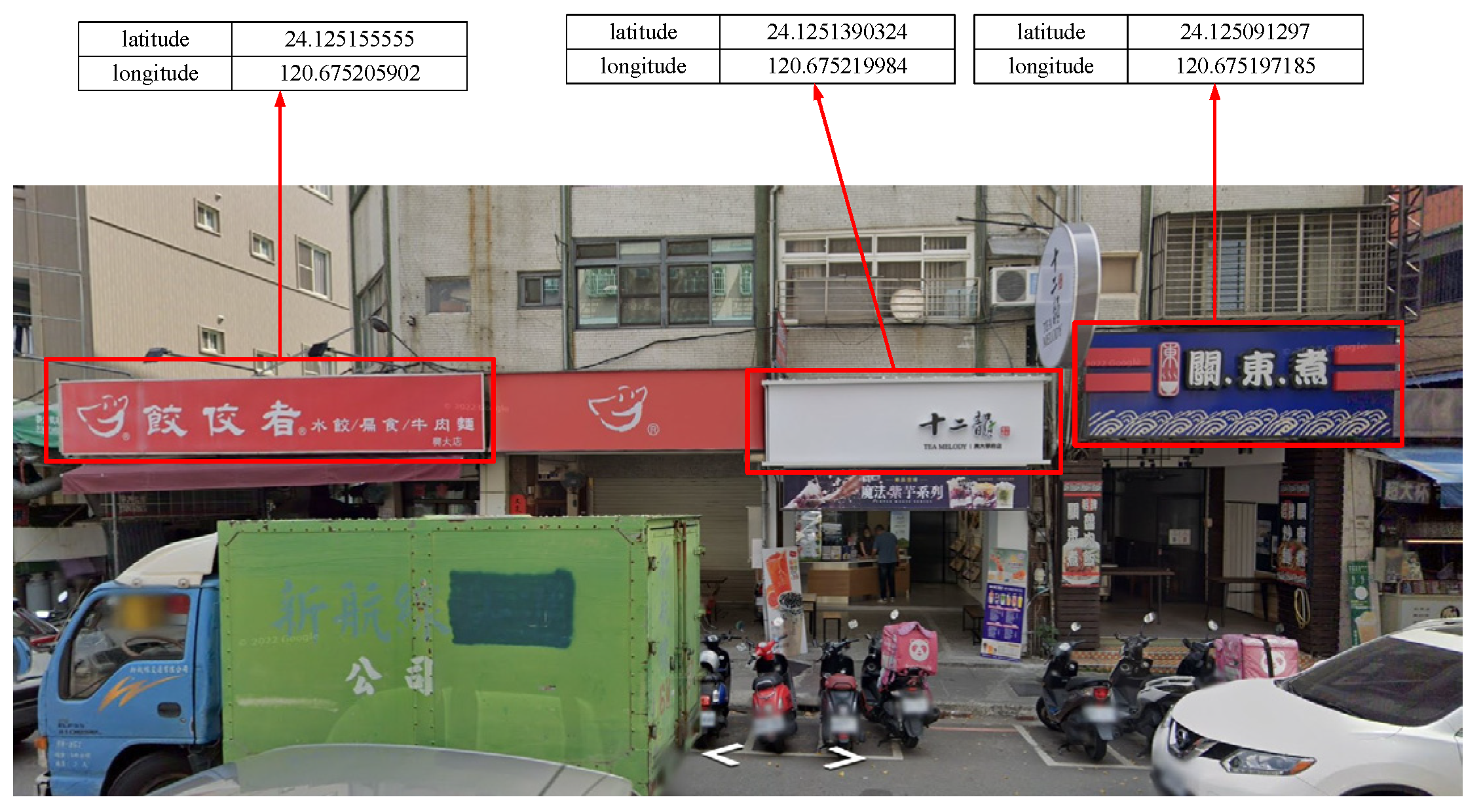
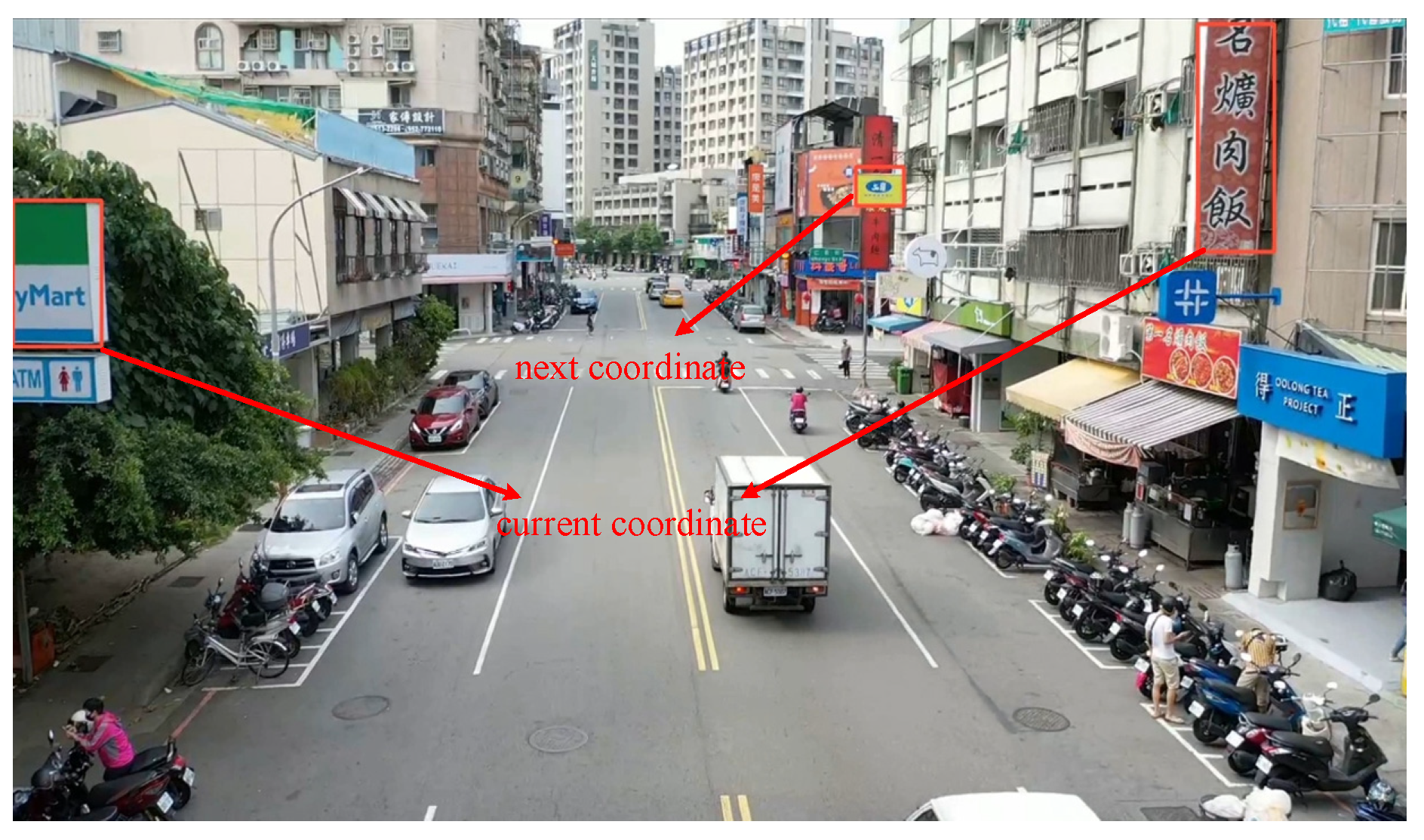
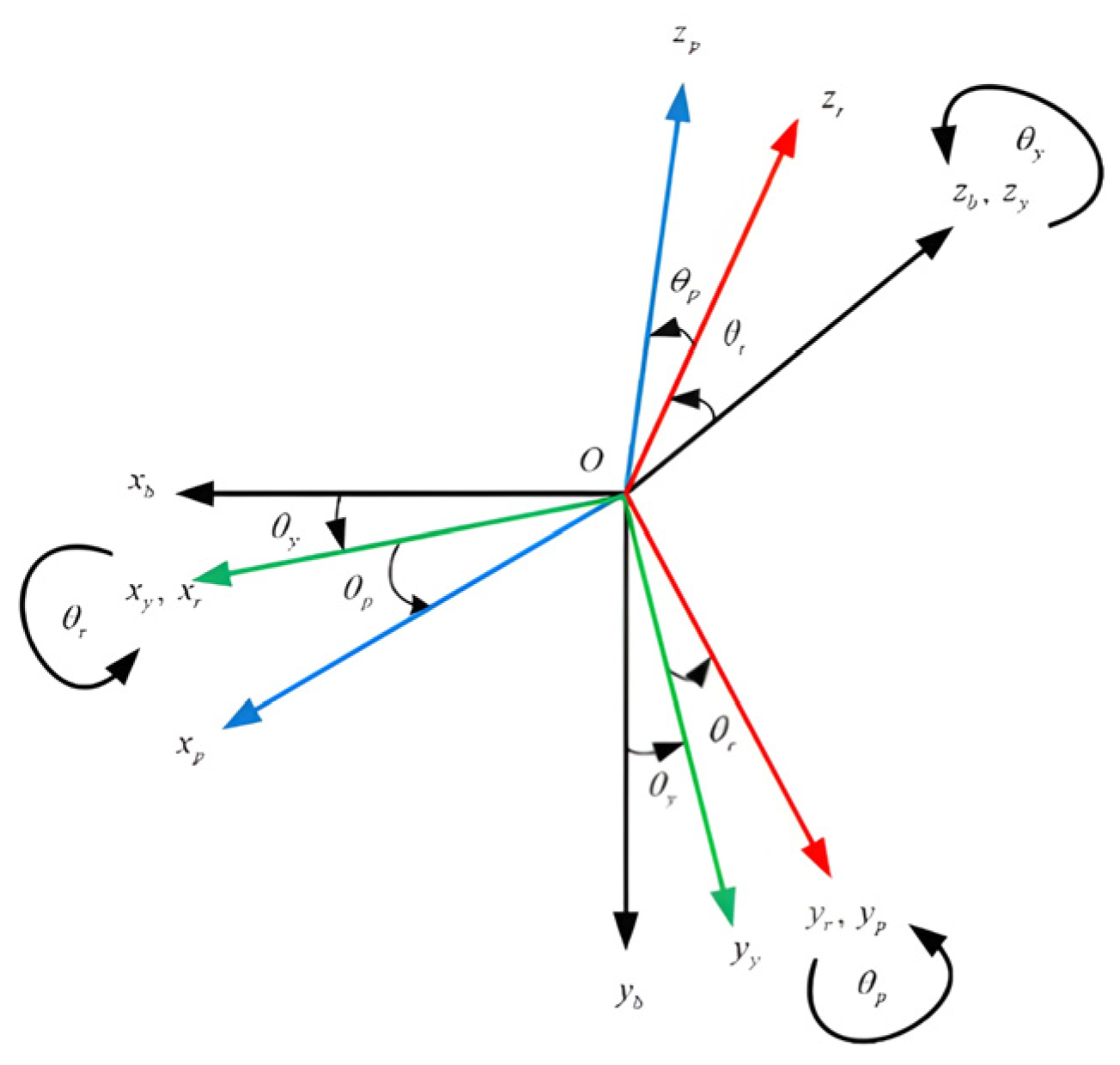
2. Locating Image Position

Accurate localization is a fundamental requirement for navigation systems, particularly in GPS-denied environments where traditional satellite-based methods are unavailable. This research proposes a system that combines image-based scene recognition, depth measurement, and inertial data fusion to achieve robust positioning. By integrating aerial and ground perspectives, the system identifies unique environmental features to support precise localization under complex conditions.

The localization framework comprises several key components. First, scene recognition algorithms, such as SIFT, are employed to extract distinctive features from captured images. These features are matched against a pre-established database to identify corresponding scene coordinates. Second, depth cameras measure the spatial distance between the camera and identified features, providing additional spatial information for improved accuracy. Third, inertial measurement units (IMUs) supply motion and orientation data, which are integrated with image-based localization through an extended Kalman filter (EKF) to ensure consistent and reliable positioning.

This section introduces the methods and techniques utilized in the system. The subsequent sections detail the processes involved in feature recognition, depth calculation, and data fusion, which collectively enable accurate and efficient localization in GPS-denied scenarios.

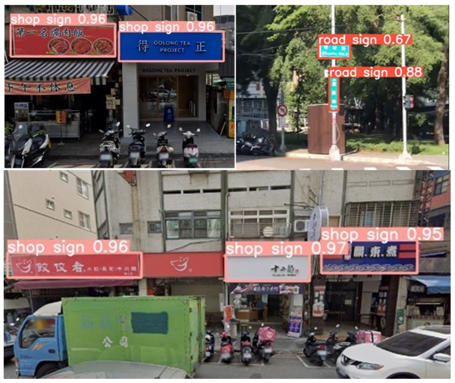
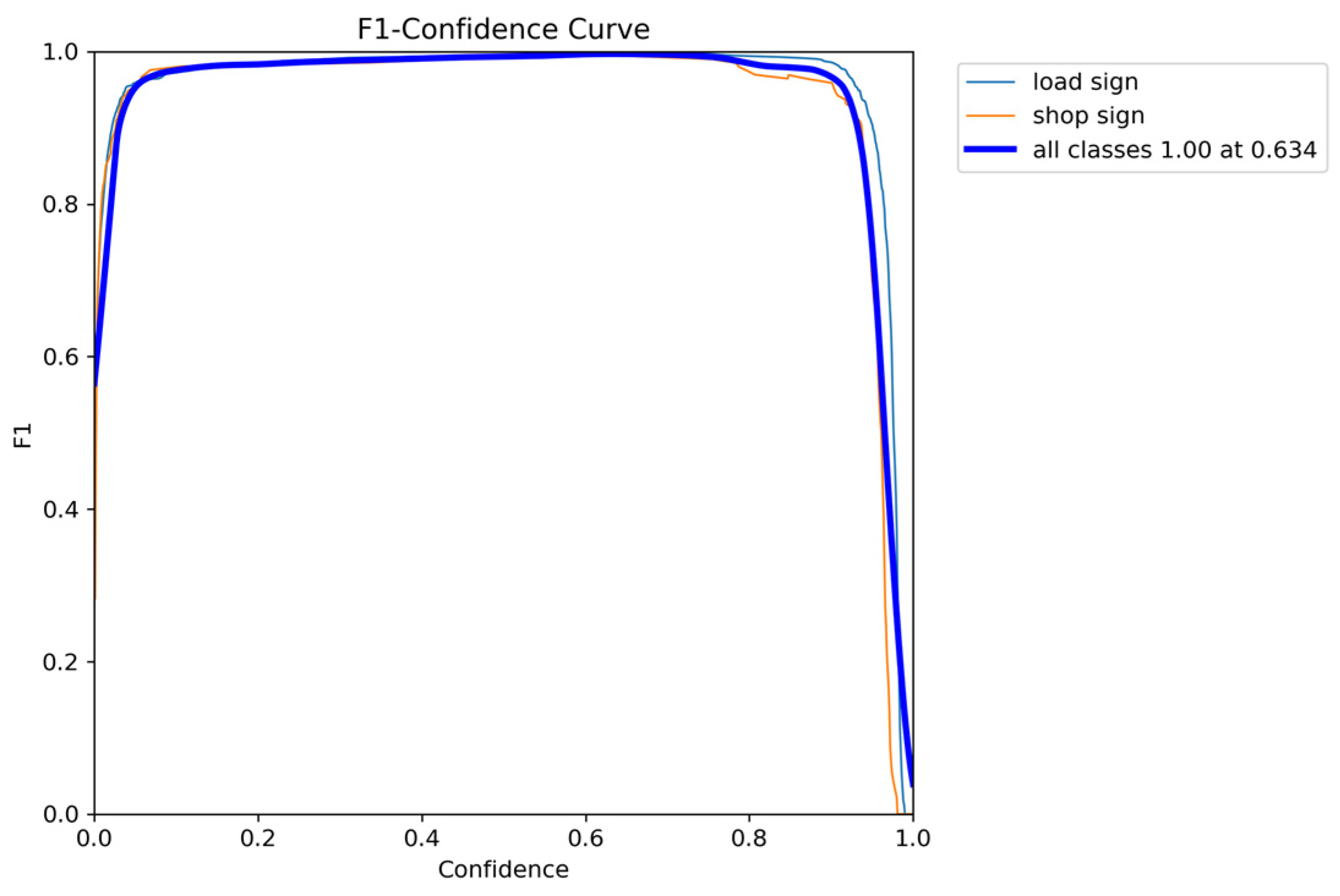
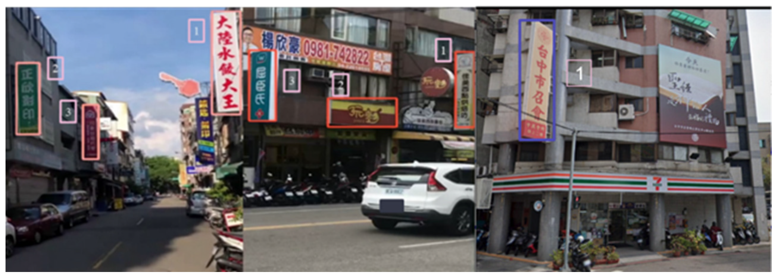
2.1. Object Recognition

As the 1980s unfolded, a range of object recognition algorithms based on feature extraction emerged. During this period, algorithms like the Canny edge detector and the Sobel filter [17] were introduced, which hinged on local image attributes. These algorithms have demonstrated their efficacy in scenarios characterized by distinct contexts, allowing for effective object recognition in these defined settings. To optimize scene recognition, selecting distinguishable features is crucial. Because extracting feature points from an entire scene is time-consuming. The focus is on identifying features such as shop signs and road signs, which are easier to distinguish in street views.

Using the PyTorch version 1.13.0 and YOLOv5 version 6.2 [18] for model training, a grid-based method was implemented to detect targets through a single neural network without predefined regions. The training dataset consisted of 1329 street images from Taiwan with 4452 labels, while the testing dataset included 24 sample images, each containing road signs or shop signs. Multiple images of the same location captured from various angles and distances are selected to ensure high recognition accuracy of street views.

After obtaining the training set images, the next step is to create labels for them. This process involves annotating objects in each image by defining bounding boxes and assigning class names. This labeling process is also referred to as annotation. Our approach categorizes street-view features into road signs and shop signs. Of course, for in-depth applications, feature information is expandable if necessary.

A combination of various features was incorporated to improve recognition. These features may be observed individually in living environments, such as electric poles, transformer boxes, flowerpots, fire hydrants, etc. However, these features collectively form a distinct set of features within a single scene. This collective recognition enhances their visibility. Figure 6 and Figure 7 show the labels for the training set, encompassing road signs, shop signs, and various features. During the experimental training, the number of epochs was set to 500.

The results of box loss, objective loss, and classification loss for the training and validation sets are recorded to show model prediction and classification accuracy. The lower the values of these parameters, the higher the consistency of the prediction results with the actual results. Precision and recall are key metrics for assessing training results and are calculated as follows [19,20,21]:

$$precision={\displaystyle \frac{TP}{TP+FP}}\cdot 100\%$$

(1)

$$recall={\displaystyle \frac{TP}{TP+FN}}\cdot 100\%$$

(2)

where TP (True Positive) is the number of actual positive samples (samples that belong to the target class) with positive predicted outcomes, FP (False Positive) is the number of actual negative samples (samples that do not belong to the target class) with positive predicted outcomes, and FN (False Negative) is the number of actual negative samples with negative prediction results. The metrics mAP@0.5 and mAP@0.5:0.9 are used to evaluate model accuracy, where mAP@0.5 indicates the accuracy when the intersection over union (IoU) threshold is 0.5, and mAP@0.5:0.9 represents the average accuracy across IoU thresholds ranging from 0.5 to 0.9. IoU refers to the ratio of the overlapping area between the predicted frame and the actual frame to their union.

Figure 8 shows the F1-score of the training model. It serves as a metric for an overall precision assessment, ranging from 0 to 1. A higher F1-score indicates better recognition performance. Ideally, an F1-score, defined below, should be as close to 1 as possible to ensure accurate and reliable results:

$$F1\mathit{-score}= 2{\displaystyle \frac{precision\cdot recall}{precision+recall}}$$

(3)

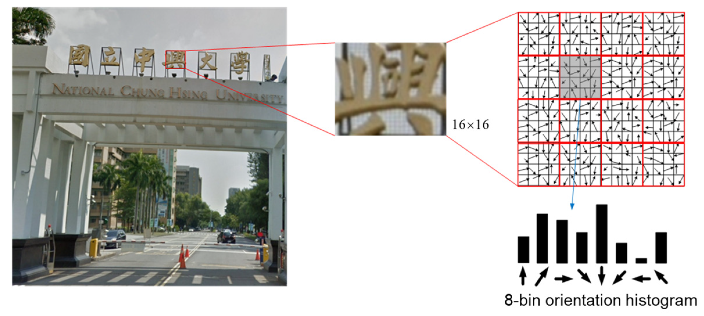
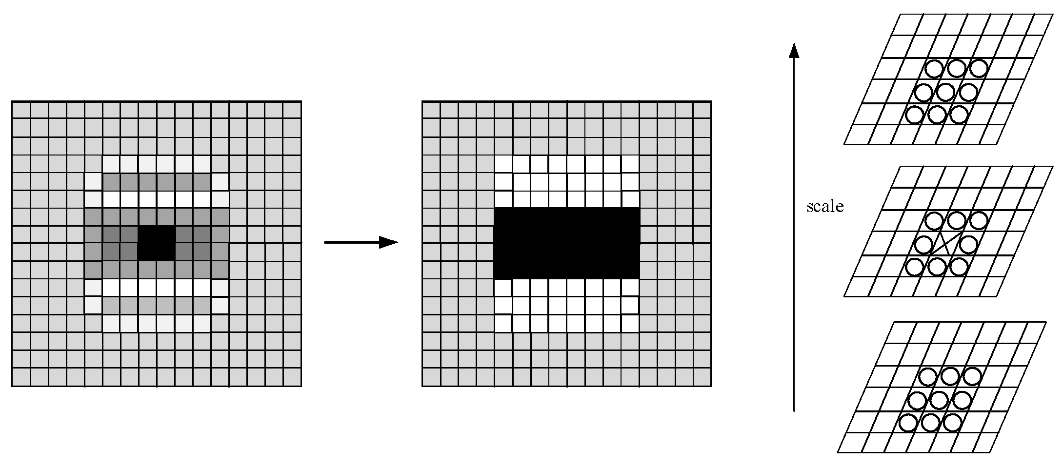
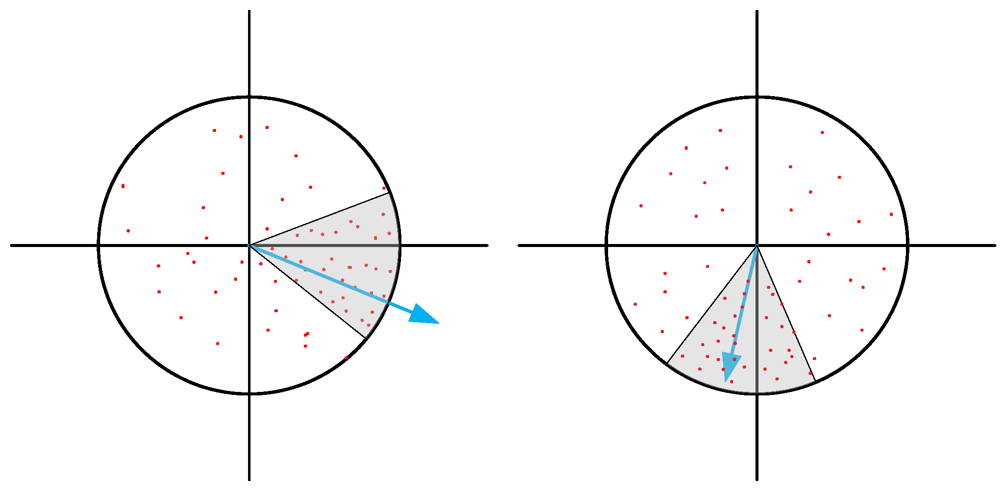
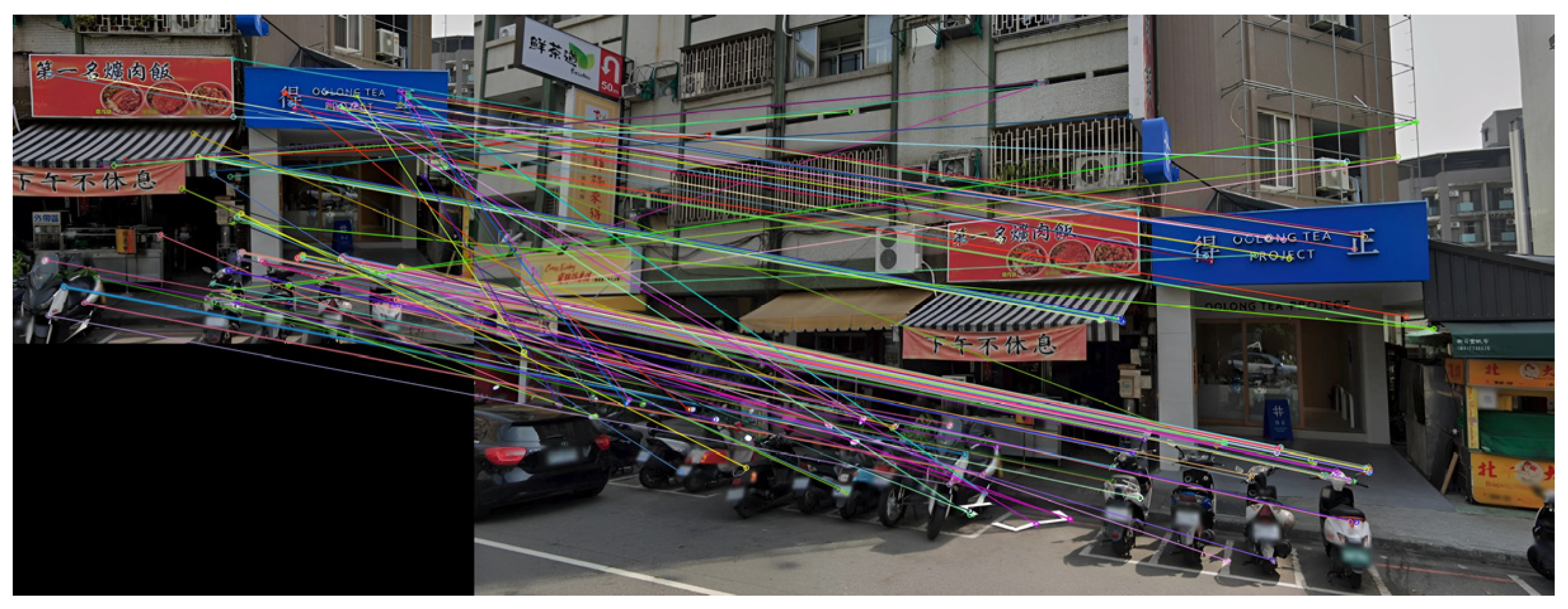
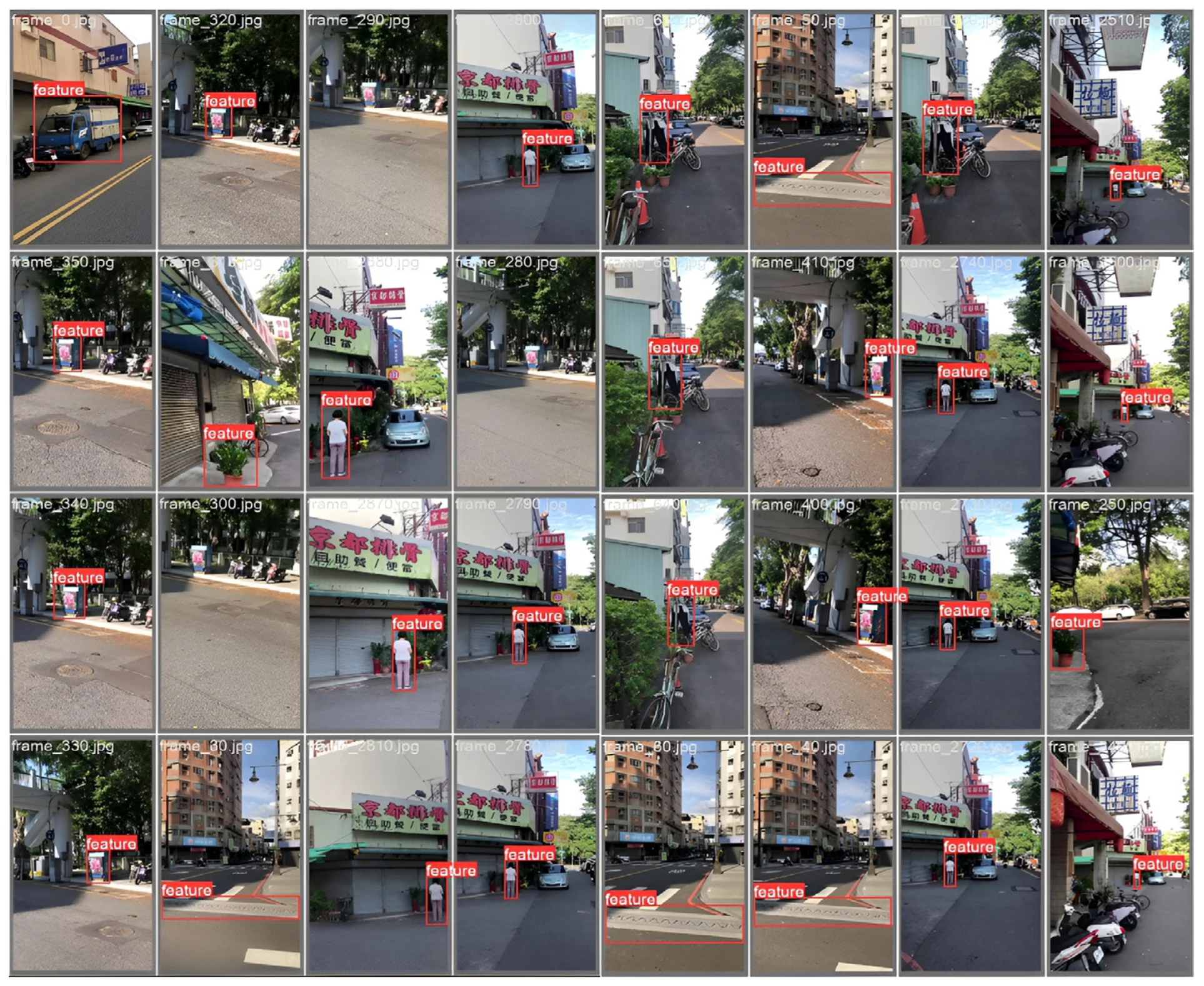
2.2. Feature Recognition

Accurate localization within the database is critical for precise positioning, particularly in GPS-denied environments. To achieve this, the system leverages a combination of advanced algorithms and cutting-edge tools. Imaging devices, such as the Intel RealSense D435I camera, capture high-resolution RGB images and provide precise depth measurements, enhancing the system’s ability to identify key environmental features and calculate spatial distances. These devices are complemented by computational platforms equipped with NVIDIA Jetson modules and desktop GPUs (e.g., NVIDIA RTX Series), enabling real-time processing and intensive algorithmic computations.

To determine the most effective feature-recognition algorithm, a comprehensive series of tests was conducted. A dataset of 1056 images, categorized by brightness levels, was utilized to evaluate performance across various lighting conditions. Feature extraction and matching were implemented using OpenCV, which provided an efficient integration of SIFT and SURF algorithms. PyTorch was employed for training additional deep learning models, enabling further optimization of feature recognition in dynamic environments.

For each image, feature points were extracted, and key metrics—such as the number of feature points, computational time, and matching accuracy—were calculated within each brightness group. The results, summarized in

Table 1. Comparison of algorithm performance for dark images.

	Number of Feature Points	Matching Accuracy (%)	Computational Time (s)
SIFT	8765	84.32	10.15
SURF	8892	82.27	4.35
ORB	10,354	74.38	3.23
Harris	6743	70.52	8.67

and

Table 2. Comparison of algorithm performance for light images.

	Number of Feature Points	Matching Accuracy (%)	Computational Time (s)
SIFT	8543	83.56	9.84
SURF	8623	82.25	4.30
ORB	9411	81.37	3.51
Harris	8953	76.55	8.54

, reveal that both SIFT and SURF algorithms exhibited robust performance under varying lighting conditions. SIFT achieved higher matching accuracy, making it suitable for applications requiring precision, while SURF demonstrated superior computational speed, ideal for real-time systems.

The implementation of these tools and algorithms was further supported by the Robot Operating System (ROS), which facilitated seamless data communication between aerial and ground components. Through these integrations, the system achieves a comprehensive and reliable framework for feature recognition, ensuring robust performance across diverse scenarios.

This study only focused on identifying prominent features, specifically shop and road signs, to expedite scene recognition. The features were selected based on two critical factors: clarity and uniqueness. First, recognition clarity was prioritized initially to ensure that trees or other elements did not obstruct the selected features. This allows for a clear view of the entire scene.

Second, uniqueness was emphasized to ensure the selection of distinctive features that were not duplicated within the same route area. For example, convenience stores were avoided as features since multiple convenience stores are typically present in the same route area. However, if this application is needed, one could incorporate nearby store signs to ensure the correctness of the identification. The number of features in each scene may vary according to the real-world scenes. The first feature to the n-th feature can be arranged according to the above conditions. As shown in Figure 9, the features within the image were labeled sequentially and stored in the database.

In practice, one may employ the YOLO training model to extract feature images. These feature images were utilized for recognition within each scene through feature extraction. Subsequently, the overall matching rate for each scene was calculated by employing the matching rate and weight equation between the features and the images stored in the database:

$$R={\displaystyle \frac{{\alpha }_1}{\beta }}(1+0.1n)+{\displaystyle \frac{{\alpha }_2}{\beta }}(1+0.1(n-1))+\cdots +{\displaystyle \frac{{\alpha }_{n-1}}{\beta }}(1+0.1)+{\displaystyle \frac{{\alpha }_n}{\beta }}$$

(4)

where ${\alpha }_n$ is the feature point of the n-th feature match, and $\beta$ is the feature point of the entire scene. Assigning a weight difference of 0.1 to each priority feature was found to yield optimal results. This decision was based on the observation that the disparity between the matching rates of these priority features remains consistently around 10%.

Our system compares each captured image and multiple features in the database for each coordinate. The matching degree is measured, starting from the first feature and progressing to the n-th feature. However, addressing recognition challenges and potential instances of incorrect recognition is essential. To mitigate this, a specified threshold is introduced, whereby images with a matching rate exceeding the threshold are input into the weight equation for further calculation.

Recognition rates for the misidentified images were normally below 60%. Therefore, a threshold level of 60 was adopted to distinguish successful and unsuccessful recognitions. Surely, the threshold level can be appropriately adjusted to reduce errors in identifying high-priority features. A threshold spectrum ranging from 60 to 90 was applied. Since the scenes in the database contained up to five unique features, a threshold boost factor of 7.5 was employed to achieve precise tuning.

Another round of comparisons using feature images from the database was conducted.

Table 3. Comparison of the SIFT and SURF algorithms.

	Number of Feature Points	Matching Accuracy (%)	Computational Time (s)
SIFT	4173	95.61	1.57
SURF	3985	86.32	1.11

presents the average number of features, the average time consumption, and the matching accuracy of the SIFT and SURF algorithms.

The comparisons show that the SIFT and SURF algorithms have similar time consumptions when combined with (4). However, SIFT outperforms SURF in terms of accuracy, making it the preferred algorithm for feature recognition in our system.

Simulated GPS coordinates were integrated with the corresponding scene images in the database. Figure 10 displays the GPS coordinates for an image paired with simulated longitude and latitude data from Google Maps, which uses the WGS84 coordinate system.

Multiple features were arranged sequentially to enhance scene recognition and consolidate the coordinates of the entire scene. Using the center equations of the polygon [22], one obtains

$$\begin{array}{l}{x}_{center}={\displaystyle \frac{1}{6A}}{\displaystyle \sum _{i=0}^{n-1}(x_i+x_{i+1})(x_i{y}_{i+1}-x_{i+1}{y}_i)},\\ y_{center}={\displaystyle \frac{1}{6A}}{\displaystyle \sum _{i=0}^{n-1}(y_i+y_{i+1})(x_i{y}_{i+1}-x_{i+1}{y}_i)}\end{array}$$

(5)

where $A={\displaystyle \frac{1}{2}}{\displaystyle \sum _{i=0}^{n-1}(x_i{y}_{i+1}-x_{i+1}{y}_i)}$ and n are the total number of features in the scene, A is the area enclosed by all the features of the current scene, $(x_i, y_i)$ is the i-th feature of the current scene, and $(x_{center}, y_{center})$ are the center coordinates of all features in the current scene. The center coordinates of all the features within the scene were calculated, and these coordinates were substituted for the individual feature coordinates. This approach compensates for the error rate associated with scene recognition compared with taking any point on the signboard, as each sign has a different size.

Following feature recognition, the image exhibiting the highest degree of correlation within the database is identified as the current scene. Subsequently, the image is utilized to obtain pre-paired coordinates.

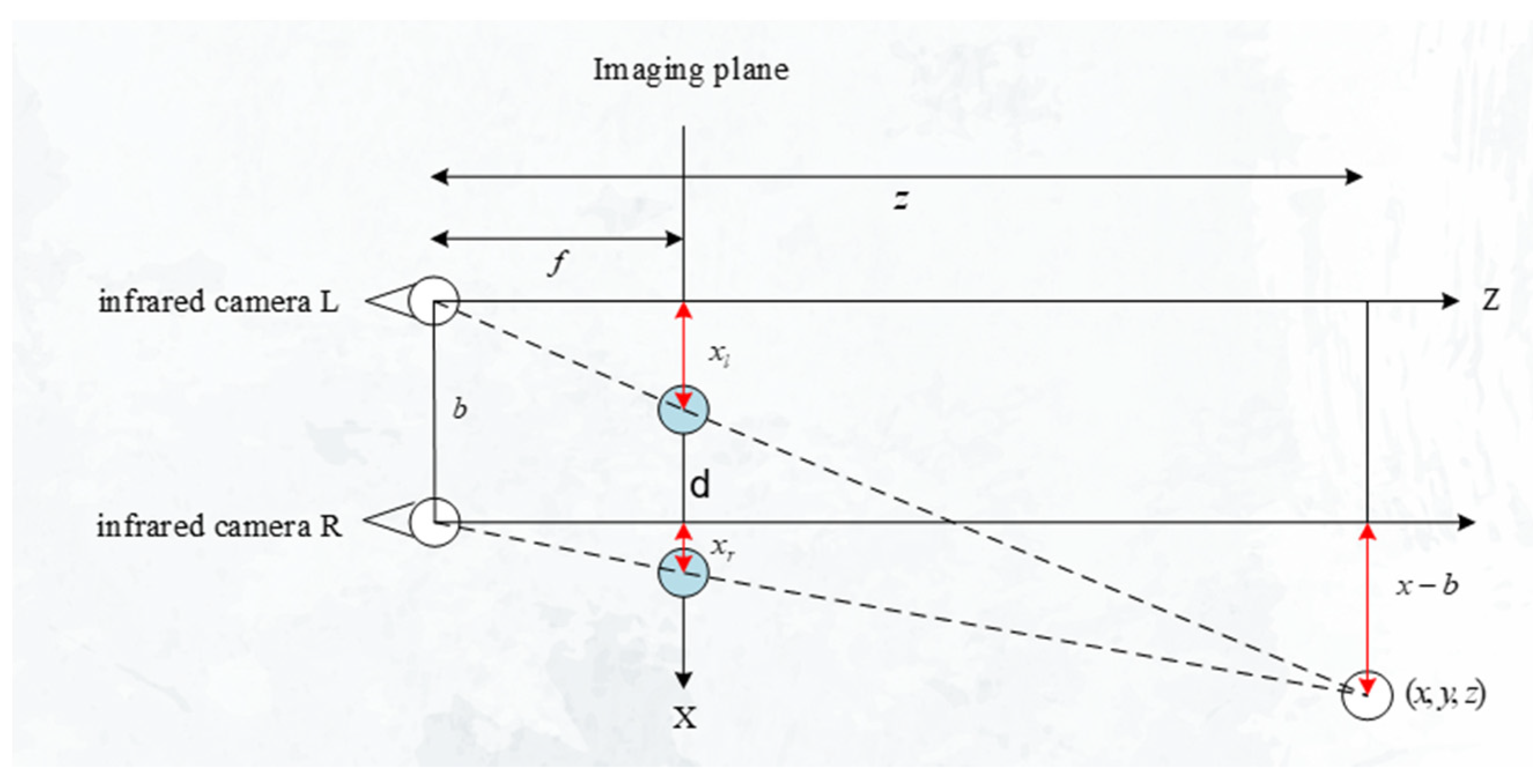
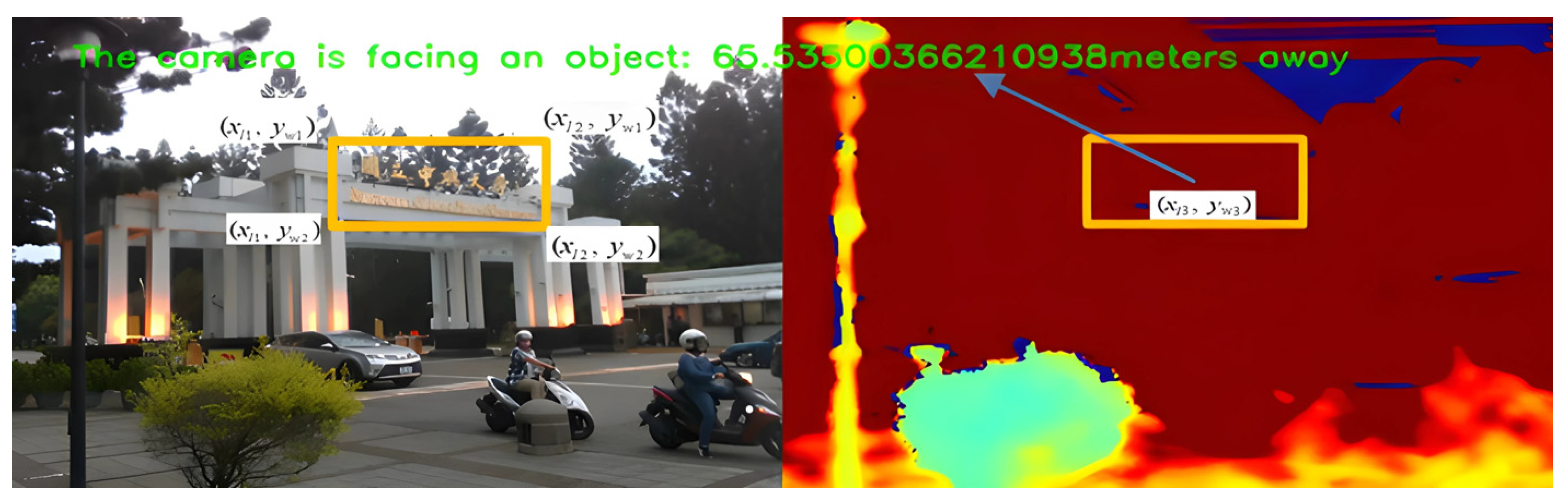
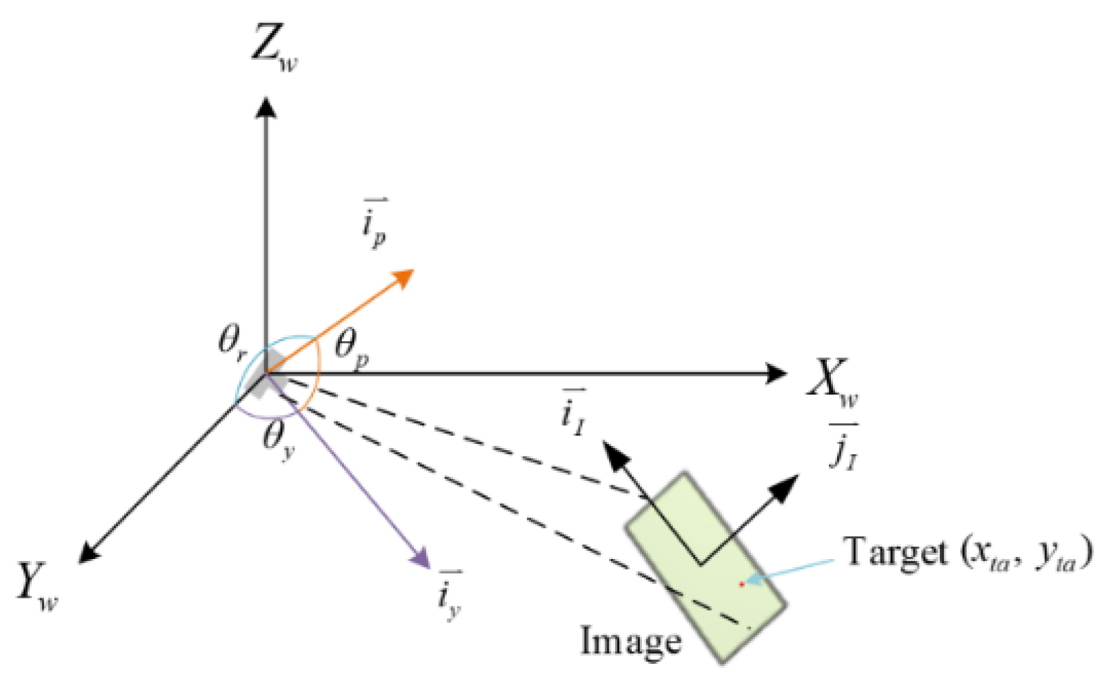
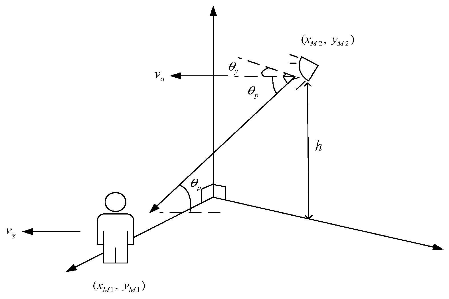
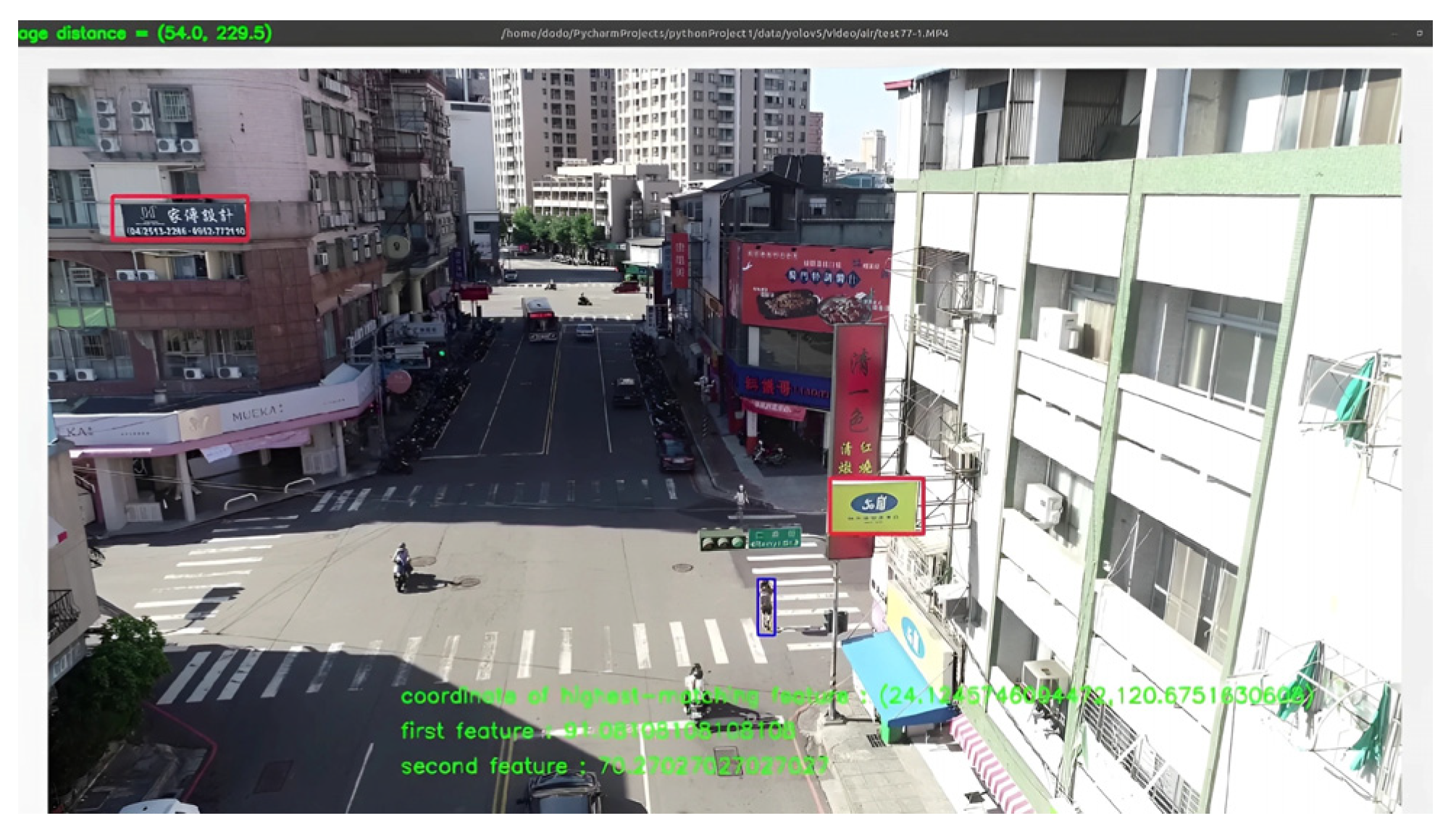
2.3. Depth Calculation

After obtaining the pre-established coordinates, the distance between the camera and the target feature is calculated to ensure precise positioning. This is accomplished using the depth camera’s left and right infrared sensors to determine the target’s depth information. Figure 11 illustrates the depth calculation process along the x-axis, with the y-axis, which is perpendicular to the figure.

The depth of the image, $z$, can be calculated using the following equation:

$$z={\displaystyle \frac{fb}{x_l-x_r}}$$

(6)

where f is the camera’s focal length, and $b$ is the length of the baseline of the left and right infrared camera lens. The composition of the depth camera involves the right and left infrared camera lens, IR projector, and RGB module. The above parameters are determined through camera calibration. In addition, $d$ is the relative distance between the pixel of the left infrared camera $(x_l, y_l)$ and the corresponding pixel of the right infrared camera $(x_r, y_r)$.

When the object frame using the training model was captured, the coordinates of the object frame in the image were used to obtain the depth of the center point of the feature and to calculate the straight distance between the camera and the feature. Figure 12 shows the actual depth map detected by the depth camera. False colors were used for easier identification. Finally, precise coordinates were obtained through the following steps:

$$x_{l3}=x_{l1}+0.5(x_{l2}-x_{l1}),y_{l3}=y_{l1}+0.5(y_{l2}-y_{l1})$$

(7)

where $(x_{l1}, y_{w1})$, $(x_{l2}, y_{w1})$, $(x_{l2}, y_{w1})$, and $(x_{l2}, y_{w2})$ are the coordinates of the object frame of the training model in the image, and $(x_{l3}, y_{w3})$ is the center coordinate of the object frame of the training model in the image. The obtained z refers to the depth of $(x_{l3}, y_{w3})$.

When the camera recognizes multiple features, several distance values are generated for a single frame. To address this, distance values corresponding to features from other scenes are filtered out. The average distance value for each feature in the current scene will be calculated, which serves as the representative distance value of the current frame. Finally, the calculated position coordinates of the camera $(x_c, y_c)$ are determined based on the depth value.

$$\left\{\begin{array}{c}\begin{array}{c}\left[\begin{array}{c}{x}_c\\ y_c\end{array}\right]=\left[\begin{array}{c}{x}_I\\ y_I\end{array}\right]+\left[\begin{array}{c}-z\\ x-b\end{array}\right], {45}^{\circ }\le {\theta }_c<{135}^{\circ }\\ \left[\begin{array}{c}{x}_c\\ y_c\end{array}\right]=\left[\begin{array}{c}{x}_I\\ y_I\end{array}\right]+\left[\begin{array}{c}x-b\\ z\end{array}\right], {135}^{\circ }\le {\theta }_c<{225}^{\circ }\end{array}\\ \begin{array}{c}\left[\begin{array}{c}{x}_c\\ y_c\end{array}\right]=\left[\begin{array}{c}{x}_I\\ y_I\end{array}\right]+\left[\begin{array}{c}z\\ -(x-b)\end{array}\right], {225}^{\circ }\le {\theta }_c<{315}^{\circ }\\ \begin{array}{c}\left[\begin{array}{c}{x}_c\\ y_c\end{array}\right]=\left[\begin{array}{c}{x}_I\\ y_I\end{array}\right]+\left[\begin{array}{c}-(x-b)\\ -z\end{array}\right],\\ {315}^{\circ }\le {\theta }_c<{360}^{\circ } \& 0^{\circ }\le {\theta }_c<{45}^{\circ } \end{array}\end{array}\end{array}\right.$$

(8)

where $(x_I, y_I)$ are the GPS coordinates for the scene image from Google Maps, and ${\theta }_c$ is the camera’s angle on the x-axis.

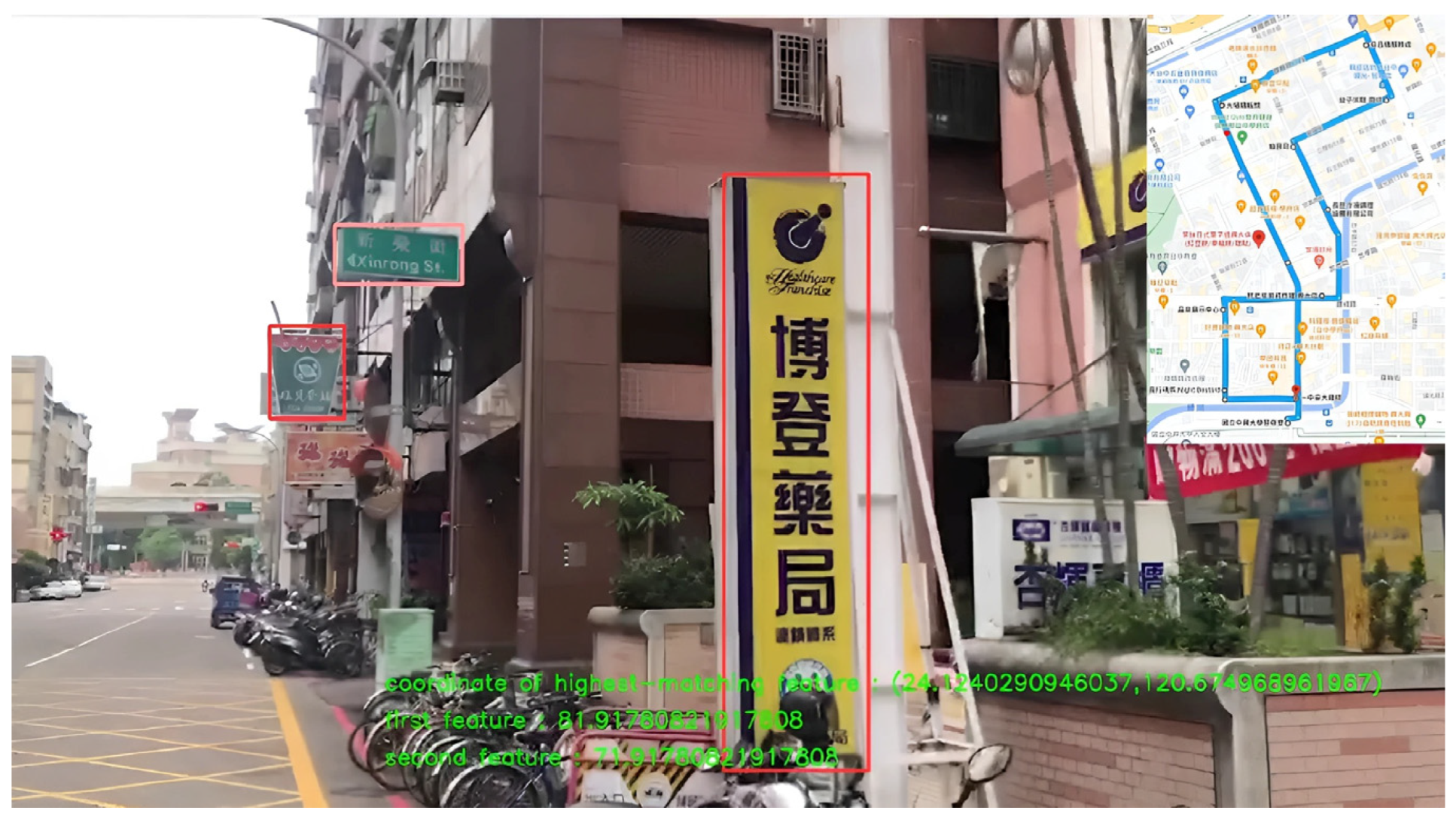
2.4. Information Fusion

When the system obtains the current coordinate, it fuses the longitude, latitude, and surrounding scene data with the IMU information and the EKF. The operational flow of the use of EKF is shown in Figure 13. It depicts that the GPS coordinates of the correct step are changed to the coordinates corresponding to the image in the database instead of the GPS coordinates of the updated phase. The angular rate and linear acceleration are extracted from the IMU. Following the integration process, the displacement and the directional angle are calculated. These are then utilized to compute the Kalman gain, which aims to predict and correct the subsequent steps. Ultimately, the positioning system iterates through these steps, making accurate predictions with the updated GPS coordinates for images and IMU. As this process is standard, the details are omitted here for simplicity.

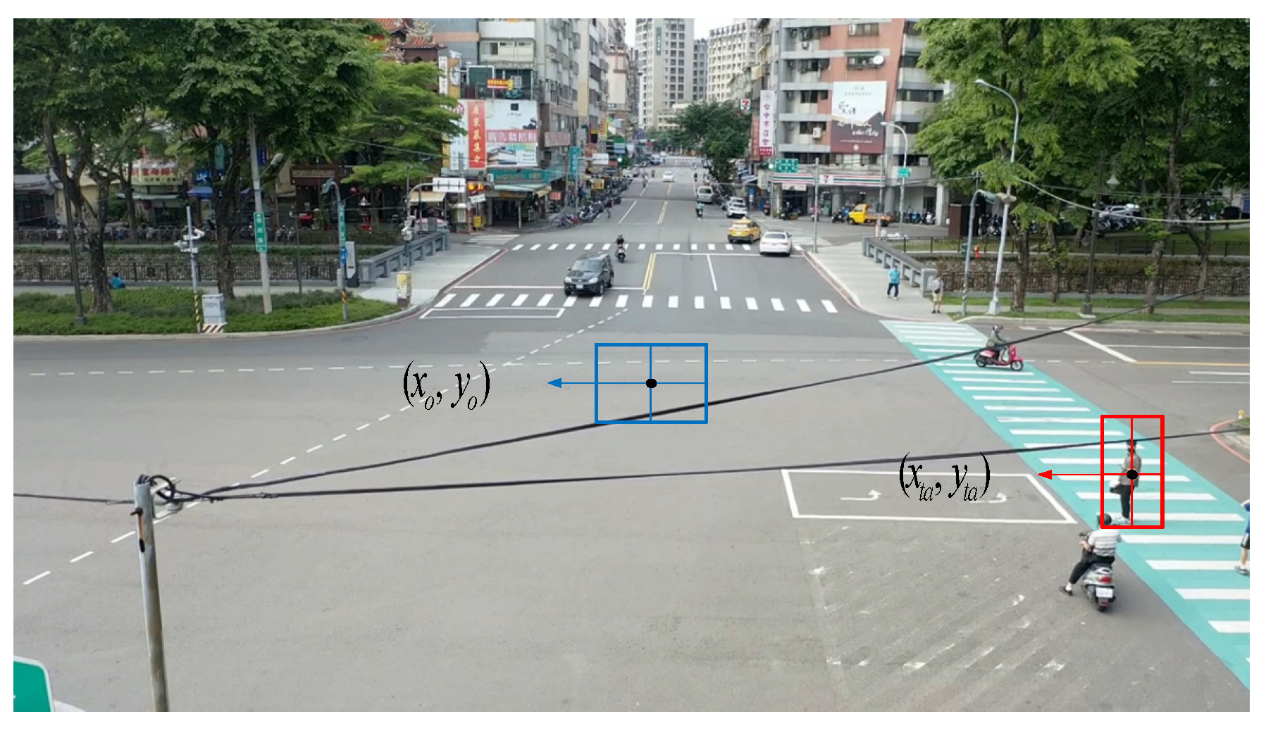
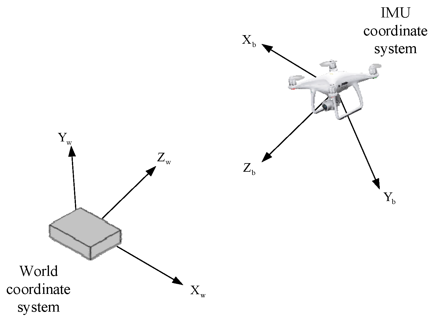
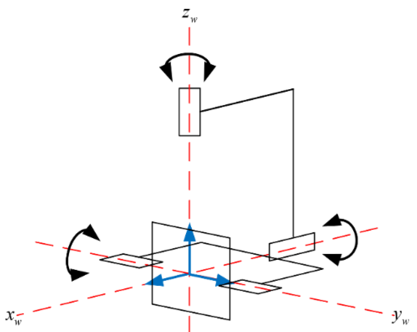
3. Design of Heterogeneous Cooperation System

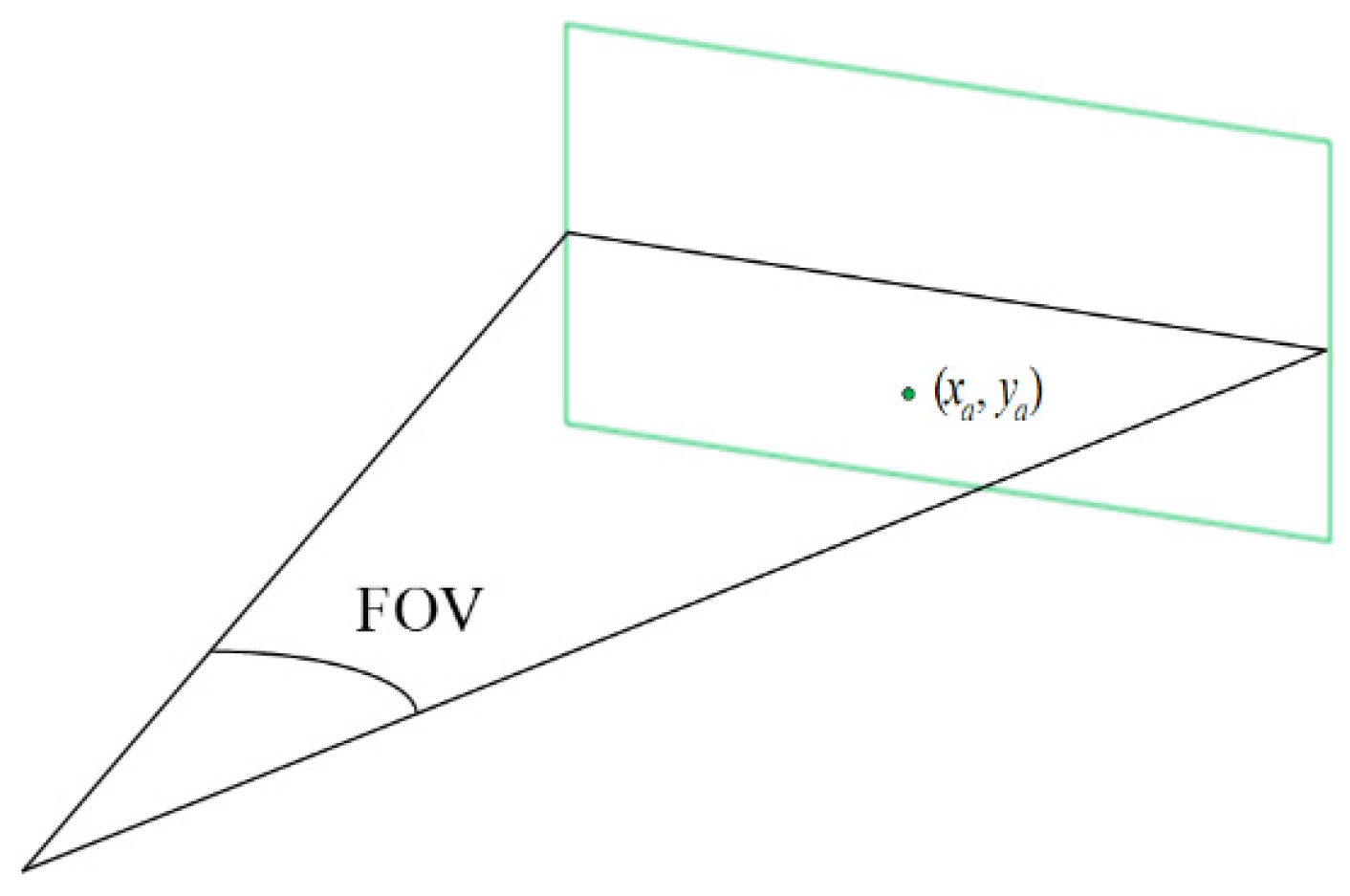
3.1. Scene Recognition in Aerial View

During real-world scene recognition, one may encounter issues related to angles or lighting conditions that hinder feature recognition. Additionally, some environments lack distinct features, such as the countryside, forests, or mountainous areas. To address these issues, it would be helpful to incorporate an aerial image to assist with scene recognition. By employing an aerial perspective, one can enhance feature recognition within a scene. Figure 14 shows the difference when roadside trees obstruct the ground view.

However, obstacles like trees and wires may appear from an aerial perspective. Additionally, at higher altitudes, the field of view in an aerial image usually contains numerous features with distinct coordinates, as illustrated in Figure 15. To accurately determine a target’s coordinates, it is essential to lock onto the specific target. One can also calculate the aerial scene’s position by referencing the ground scene’s coordinate position to enable effective heterogeneous coordination.

According to the first equation [23], the fixed focal length and object size in the photo are proportional to the depth of the object and its real-world size. Thus, since the camera configured on the UAV cannot obtain depth values, it is possible to estimate the size $S_{feature}$ of a feature based on the depth value of the feature, as follows:

$$S_{feature}={\displaystyle \frac{z_{ground}{p}_{ground}}{f_{depth}}}$$

(9)

where $f_{depth}$ is the focal length of the depth camera, $z_{ground}$ is the depth value of the center of the feature detected by the depth camera, and $p_{ground}$ is the pixel size occupied by the feature in the RGB image of the depth camera. The actual size value of the feature can be used to calculate the distance between a UAV camera and a feature:

$$z_{aerial}={\displaystyle \frac{S_{feature}{f}_{UAV}}{p_{aerial}}}$$

(10)

where $z_{aerial}$ is the calculated distance between the center of the feature and the UAV’s camera, $f_{UAV}$ is the focal length of the UAV’s camera, and $p_{aerial}$ is the pixel size occupied by the feature in the image of the UAV’s camera.

3.2. Heterogeneous Location Calculation and Camera Tracker

When obtaining current GPS coordinates through a UAV, it is vital to consider the UAV’s extensive field of view, which may cover multiple GPS coordinates. To ensure accurate positioning, the position of the target is used to constrain the range of UAV coordinates, allowing the precise location of the current coordinates to be confirmed. Therefore, it is crucial to ascertain the relative position of the UAV and the target. Figure 16 displays the positional relationship between the screen center and the target.

In Figure 16, the mark $( x_o, y_o)$ denotes the center coordinates of the camera screen, and $( x_{ta}, y_{ta})$ are the center coordinates of the target on the camera screen. Before initiating the calculation, it is necessary to transform the coordinates by converting the UAV’s coordinate system to align with the target’s coordinate system.

Figure 17 illustrates the coordinate system of the IMU on the UAV and the coordinate system of the target. The global coordinate system is $(X_W, Y_W, Z_W)$, and the UAV’s inertial coordinate system is $(X_b, Y_b, Z_b)$.

Figure 18 and Figure 19 illustrate the camera gimbal’s structure and coordinate conversion diagrams. Here, ${\theta }_y, {\theta }_p$, and ${\theta }_r$ are, respectively, the yaw, pitch, and roll angles of the camera gimbal, and $(x_y, y_y, z_y), (x_p, y_p, z_p)$, and $(x_r, y_r, z_r)$ are, respectively, the coordinates for the yaw, pitch, and roll rotation axes. One can then perform coordinate transformations based on the camera gimbal’s pitch, yaw, and roll rotation axes.

The coordinate transformation matrix of the inertial coordinate system to the global coordinate system [24] and the three-axis rotation matrix of the camera gimbal in the order of roll, yaw, and pitch rotations are given by

$${\left[\begin{array}{l}x\\ y\\ z\end{array}\right]}_w=R({\theta }_y)R({\theta }_p)R({\theta }_r){\left[\begin{array}{l}x\\ y\\ z\end{array}\right]}_b$$

(11)

where $R({\theta }_y)=\left[\begin{array}{ccc}\cos {\theta }_y& \sin {\theta }_y& 0\\ -\sin {\theta }_y& \cos {\theta }_y& 0\\ 0& 0& 1\end{array}\right], R({\theta }_p)=\left[\begin{array}{ccc}\cos {\theta }_p& 0& -\sin {\theta }_p\\ 0& 1& 0\\ \sin {\theta }_p& 0& \cos {\theta }_p\end{array}\right], R({\theta }_r)=\left[\begin{array}{ccc} 1& 0& 0\\ 0& \cos {\theta }_r& \sin {\theta }_r\\ 0& -\sin {\theta }_r& \cos {\theta }_r\end{array}\right]$.

Next, the IMU coordinate system acquires the measured angular velocities along the three rotation axes. Utilizing Equation (12), the angles for these three rotation axes are as follows:

$$\left[\begin{array}{c}{\theta }_r\\ {\theta }_p\\ {\theta }_y\end{array}\right]={\displaystyle \int \left[\begin{array}{ccc}1& \sin {\theta }_r\tan {\theta }_p& \cos {\theta }_r\tan {\theta }_p\\ 0& \cos {\theta }_r& -\sin {\theta }_r\\ 0& \frac{\sin {\theta }_r}{\cos {\theta }_p}& \frac{\cos {\theta }_r}{\sin {\theta }_p}\end{array}\right]\left[\begin{array}{c}{\omega }_{X_b}\\ {\omega }_{Y_b}\\ {\omega }_{Z_b}\end{array}\right]} dt$$

(12)

Field of view (FOV) dimensions play a crucial role in determining the range of the observed scene. In this setup, as shown in Figure 20, the FOV is defined by the lens’s focal length and the sensor’s size. It is important to note that different lenses and cameras can result in varying FOVs.

Let the image dimensions be $W\times H$ (e.g., 1920 × 1080) pixels and the position of the target in the image be denoted by $( x_{ta}, y_{ta})$. Given that the ratio of the image width to the distance from the lens to the image center is proportional to the tangent of the FOV, the distance from the lens to the image center is designated as the unit length. The relative position between the target image and the image center is defined as follows:

$$\left[\begin{array}{c}x\\ y\\ z\end{array}\right]={\left[\begin{array}{c}2{\displaystyle \frac{x_{ta}}{W}}\tan \left({\displaystyle \frac{FOV}{2}}\right)\\ 2{\displaystyle \frac{y_{ta}}{W}}\tan \left({\displaystyle \frac{FOV}{2}}\right)\\ 1\end{array}\right]}_I$$

(13)

Figure 21 illustrates the relationship between the target within the image and the global coordinate system. Here, $\stackrel{\rightharpoonup }{i_I}$ and $\stackrel{\rightharpoonup }{j_I}$ are unit vectors in the x and y directions of the image, and $\stackrel{\rightharpoonup }{i_p}$ and $\stackrel{\rightharpoonup }{i_y}$ are the unit vectors of the pitch and yaw directions of the camera gimbal. It can be seen from the relationship diagram that the conversion relationship between the camera gimbal and the yaw rotation axis is as follows:

$${\left[\begin{array}{l}x\\ y\\ z\end{array}\right]}_w=\left[\begin{array}{l}1\\ 0\\ 0\end{array}\right]+R_I{\left[\begin{array}{l}x\\ y\\ z\end{array}\right]}_I$$

(14)

where $R_I=\left[\begin{array}{ccc}0& 0& 1\\ -1& 0& 0\\ 0& 1& 0\end{array}\right]$.

The coordinates of the image target can now be obtained through the following transformation:

$${\left[\begin{array}{c}x\\ y\\ z\end{array}\right]}_W=2R({\theta }_y)R({\theta }_p)R({\theta }_r)R_I{\left[\begin{array}{c}{\displaystyle \frac{x_{ta}}{W}}\tan \left({\displaystyle \frac{FOV}{2}}\right)\\ {\displaystyle \frac{y_{ta}}{W}}\tan \left({\displaystyle \frac{FOV}{2}}\right)\\ 0.5\end{array}\right]}_I$$

(15)

The target’s yaw and pitch angles, relative to the camera gimbal’s coordinate system, are determined by calculating the corrected commands based on the translation and pitch angles, thereby enabling accurate tracking of the image target.

3.3. Position Conversion

The yaw and pitch angles of the camera gimbal are obtained. Let the coordinates of the UAV and the target be denoted as $(x_{M2},{ \mathrm{y}}_{M2})$ and $(x_{M1},{ \mathrm{y}}_{M1})$. The coordinates of the UAV and the target are calculated using the positional relationship between the UAV and the target, as illustrated in Figure 22 and expressed by the following equation:

$$\left[\begin{array}{c}{x}_{M2}\\ y_{M2}\end{array}\right]=\left[\begin{array}{c}{x}_{M1}\\ y_{M1}\end{array}\right]+\left[\begin{array}{c}\sin ({\theta }_y)\\ \cos ({\theta }_y)\end{array}\right] h\cot ({\theta }_p)$$

(16)

However, it is essential to note that the conversion assumes a static state. In real-world scenarios, the UAV and the ground target are mostly in motion at different speeds. To account for this, angular acceleration and linear acceleration data obtained from the IMU are incorporated to correct the relative position between the UAV and the target. By measuring the linear accelerations $a_{aerial}$ and $a_{ground}$ using the accelerometers in the ground target’s IMU and the UAV’s IMU, the angular velocities ${\omega }_{yaerial}$, ${\omega }_{yground}$, ${\omega }_{paerial}$, and ${\omega }_{pground}$ of the yaw and pitch axes can be obtained from the gyroscopes in the UAV and the target’s IMU, respectively. The velocity and angular changes during the period between time instants $t_0$ to $t_1$ are measured to calculate the relative position as follows:

$$\begin{array}{l}\Delta v={\displaystyle {\int }_{t_0}^{t_1} (a_{ground}-a_{aerial}) dt},\\ \Delta {\theta }_y={\displaystyle {\int }_{t_0}^{t_1}}({\omega }_{yground}-{\omega }_{yaerial}) dt,\\ \Delta {\theta }_p={\displaystyle {\int }_{t_0}^{t_1}}({\omega }_{pground}-{\omega }_{paerial}) dt\end{array}$$

(17)

which gives

$$\left[\begin{array}{c}{x}_{M1}\\ y_{M1}\end{array}\right]=\left[\begin{array}{c}{x}_{M2}\\ y_{M2}\end{array}\right]-\left[\begin{array}{c}\sin (\Delta {\theta }_y)\\ \cos (\Delta {\theta }_y)\end{array}\right]h\cot (\Delta {\theta }_p)-\left[\begin{array}{c}{\displaystyle {\int }_{t_0}^{t_1}\Delta v\sin (\Delta {\theta }_y) dt}\\ {\displaystyle {\int }_{t_0}^{t_1}\Delta v\cos (\Delta {\theta }_y) dt}\end{array}\right]$$

(18)

Equations (17) and (18) provide a solution to the problem of being unable to identify the current scene coordinates accurately, thus achieving the purpose of heterogeneous collaboration.

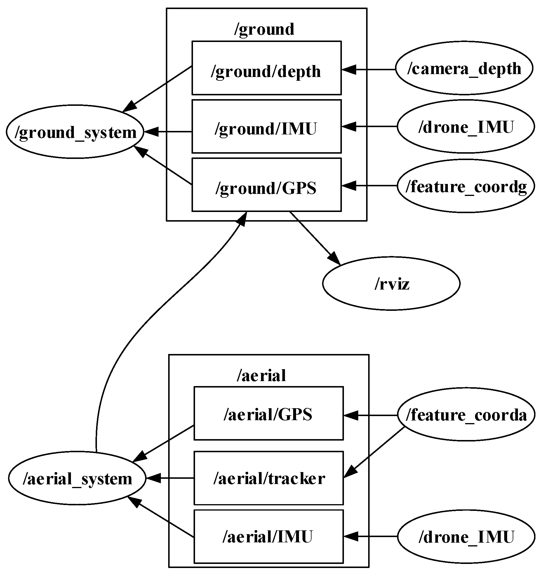
3.4. ROS Data Transfer

The publishing and subscribing functions in the Robot Operating System (ROS) [25] are used to realize the information transfer between the systems. Figure 23 illustrates the publish-and-subscribe relationship between topics and nodes. Aerial information is published to the aerial system node, allowing the ground GPS topic to subscribe and receive the transmitted data, thereby enabling a heterogeneous collaborative system. The RViz package is utilized in ROS to display route records.

3.5. Complete System Architecture

Figure 24 illustrates the comprehensive operational architecture of the proposed system, which is designed to seamlessly integrate multiple data sources for robust positioning in GPS-denied environments. The system operates through four primary components, beginning with the continuous capture of aerial and ground images using cameras for real-time scene recognition. This dual-perspective approach enhances the system’s ability to identify key features in complex environments. To accurately locate the camera’s position, SIFT feature matching is applied to compare captured images with a pre-established database, enabling the identification of the best-matching scene and extraction of corresponding GPS coordinates. A threshold-based filtering mechanism is employed to eliminate images with low matching scores, minimizing the likelihood of incorrect matches and ensuring reliable feature recognition.

The depth camera simultaneously records depth values of scene features, which are used to calculate the distance between the camera and key features. This information is critical for precise localization, as it provides an additional layer of spatial context to support navigation tasks. Finally, the system integrates data from feature matching and depth calculations with inertial measurements obtained from the IMU using an extended Kalman filter (EKF). This fusion process establishes a closed-loop architecture, ensuring stable and accurate positioning even in the absence of GPS signals.

4. Experiment

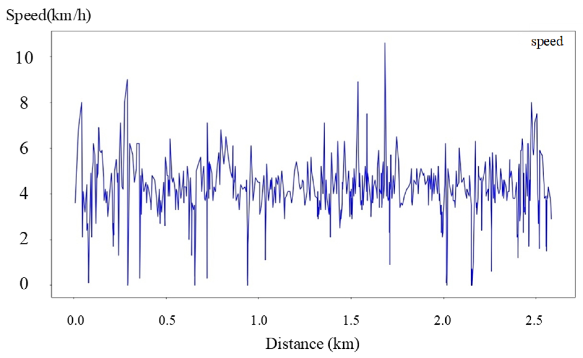
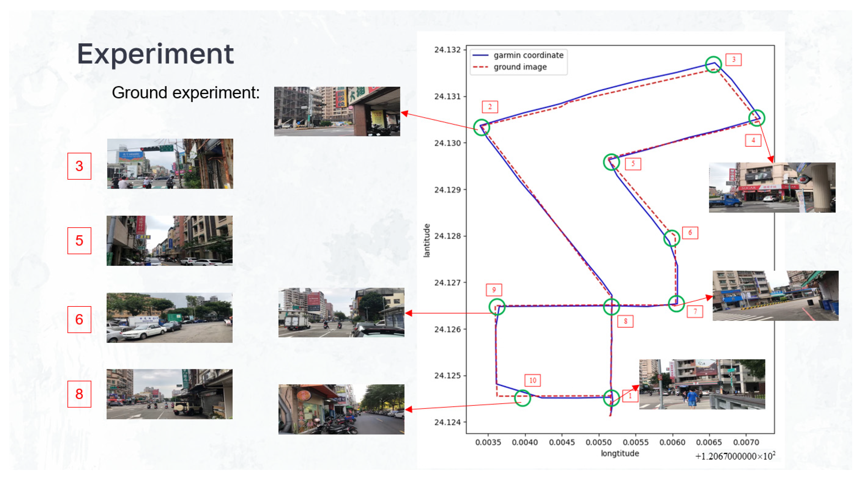
4.1. Ground Experiment

For comparison, Google’s 360° street-view images (Google LLC, Mountain View, CA, USA), which include established coordinate data, were utilized. By concentrating on specific feature identification, the number of key points required for comparison was reduced, thereby speeding up coordinate determination. In our experimental setup, a depth camera Intel RealSense D435i (Intel Corporation, Santa Clara, CA, USA) scans the surrounding scene. Equipped with an integrated IMU, this camera captures real-time linear acceleration and angular rate information. Figure 25 shows a sample image captured by the ground camera during operation. This scene is matched with database images to determine its coordinates, with the resulting matching rate and coordinates displayed on the screen. The matching process was performed using OpenCV version 4.5.5

To illustrate, coordinated information of a sampled road section was input into Google Maps, as shown in Figure 25, and the ground-view positioning algorithm was tested on the same road. Figure 26 shows our walking speed while capturing the ground scene. Figure 27 shows the depth values between the features and the camera. The experimental results for the ground view are shown in Figure 28. These figures displayed flight data of the UAV, the user’s walking status, and image responses of the real-world tests that were used for evaluating the navigation system’s performance.

The experimental results demonstrate the feasibility of the proposed algorithm. While selecting the feature set, each feature must be accurately identified for the recognition to be considered successful. As a result, the recognition rate for the feature set is comparatively lower than that of the shop signs and road signs. The position error of the corner is slightly greater than that of the straight line, and further analysis of Figure 28 reveals potential causes. To determine the orientation at the corner of the intersection, the ground camera will rotate left and right to collect more feature information about the intersection. However, store or road signs are sometimes only set on the opposite or one side, such as points 3, 6, 9, and 10. The image GPS analysis obtained from algorithms will use distant points as auxiliary positioning information. The rapid changes in camera speed and rotations during identifying scene features may have contributed to recognition instability.

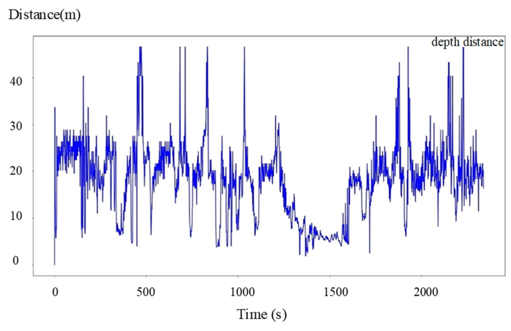
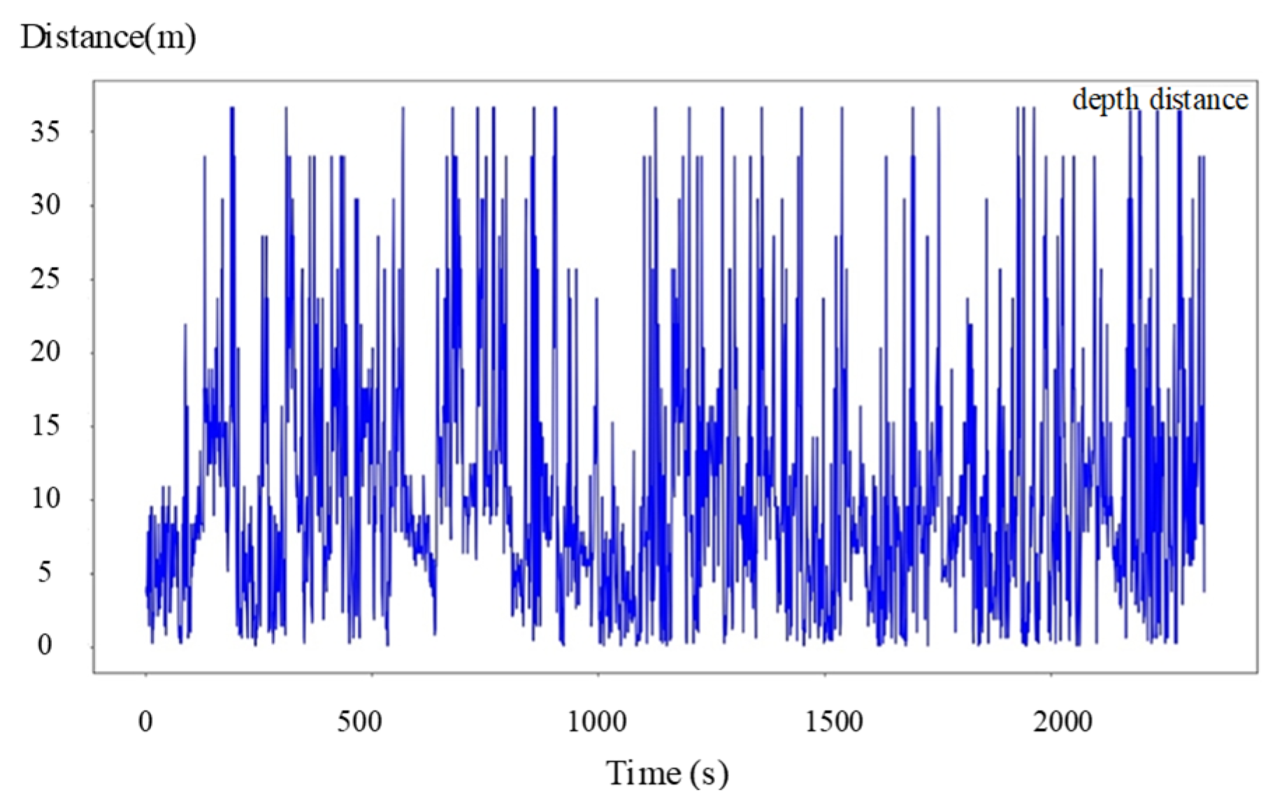
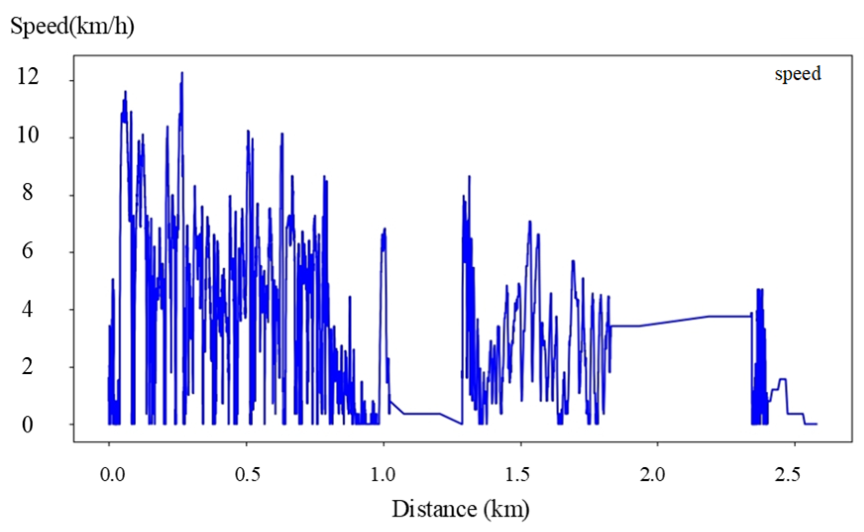
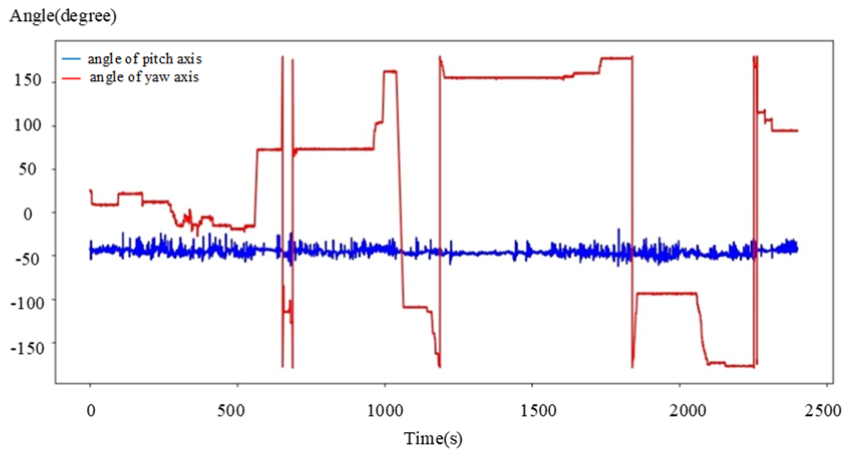
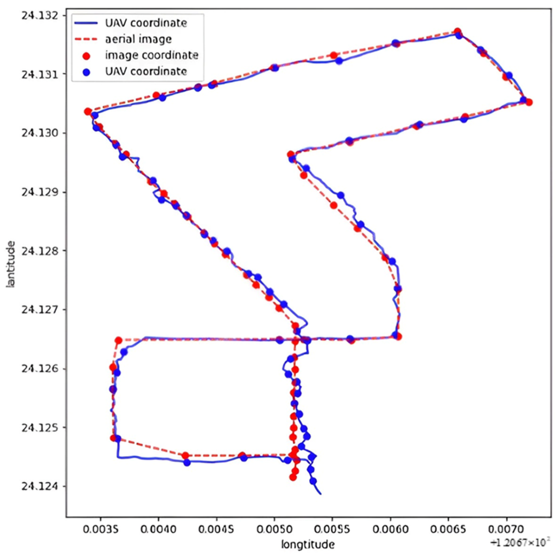
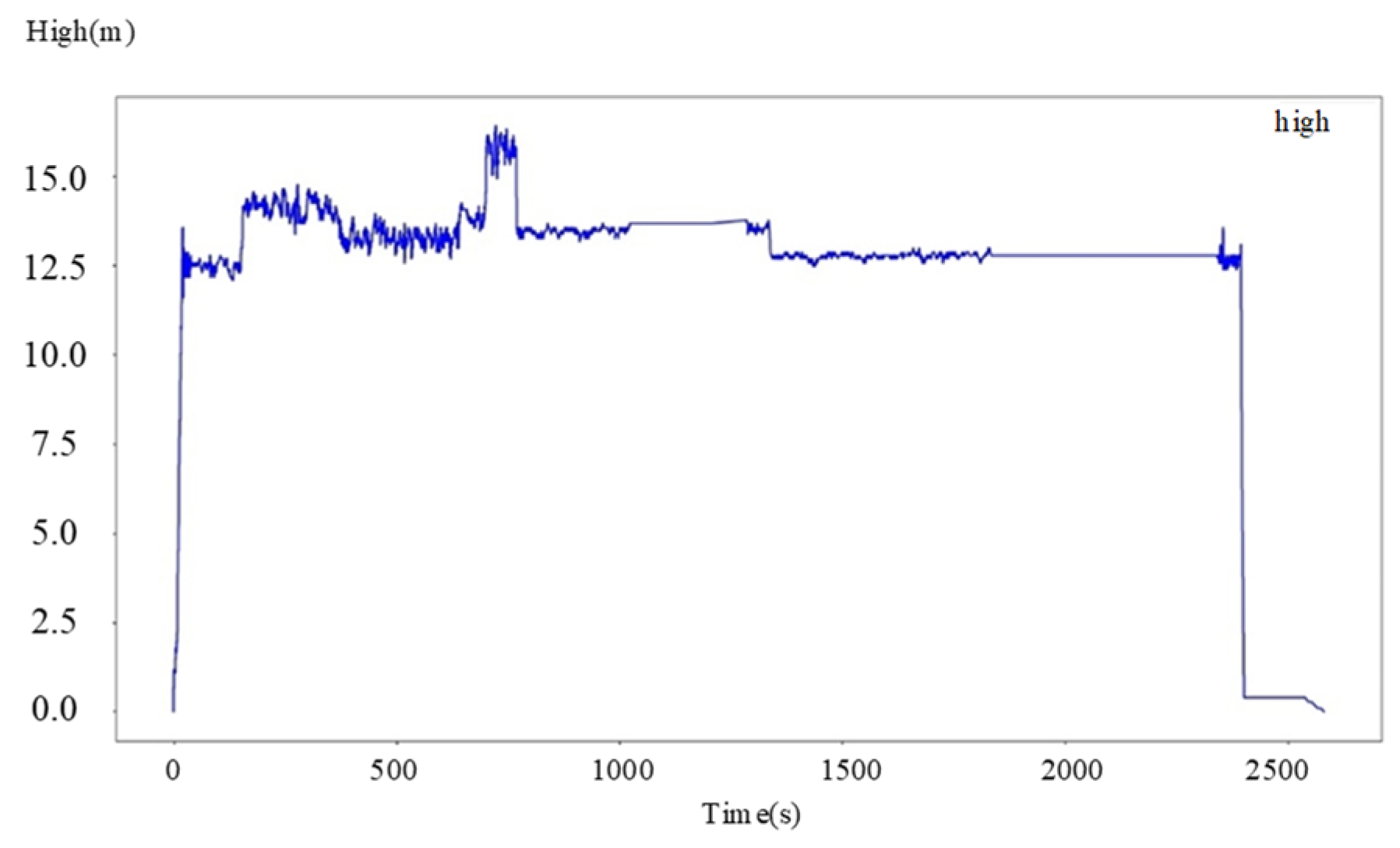
4.2. Aerial Experiments

The coordinate information shown in Figure 25 was input into the established map to test the proposed ground-positioning algorithm. Figure 29 presents sample images captured by the aerial camera during operation. In aerial scene recognition, the GPS signal coordinates of the UAV combine with coordinates obtained through scene recognition in the air. Figure 30 illustrates the distance values between the UAV camera and the recognized features, and Figure 31 depicts the flight speed of the UAV during scene capture. Figure 32 shows the UAV camera’s pitch and yaw angles, ranging from −180° to 180°. A large change in the yaw angle can be indicated when encountering an intersection. Figure 33 presents the aerial experimental results.

This instability is attributed to significant fluctuations in UAV speed, which adversely affect the overall performance of scene recognition. Additionally, as illustrated in Figure 34, the angle change of the UAV camera on the yaw axis is significant, which suggests that the excessive sensitivity of aerial recognition to changes in the camera gimbal’s angle led to unexpected variations in the coordinates along routes with frequent angle changes. The coordinates of the aerial experiment are shown in Figure 33, and the 60 points from Figure 33 are used to measure the GPS error, as illustrated in Figure 34.

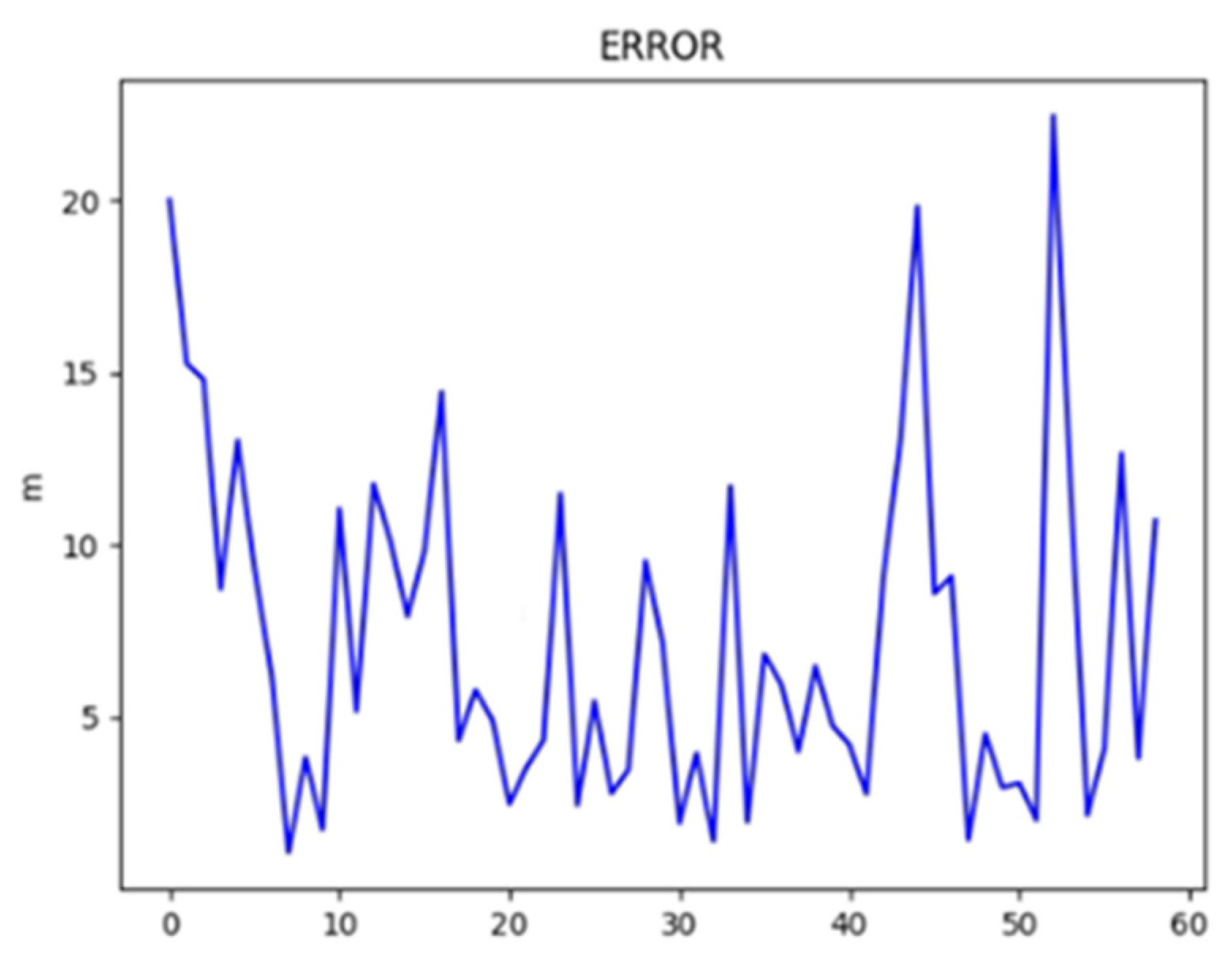
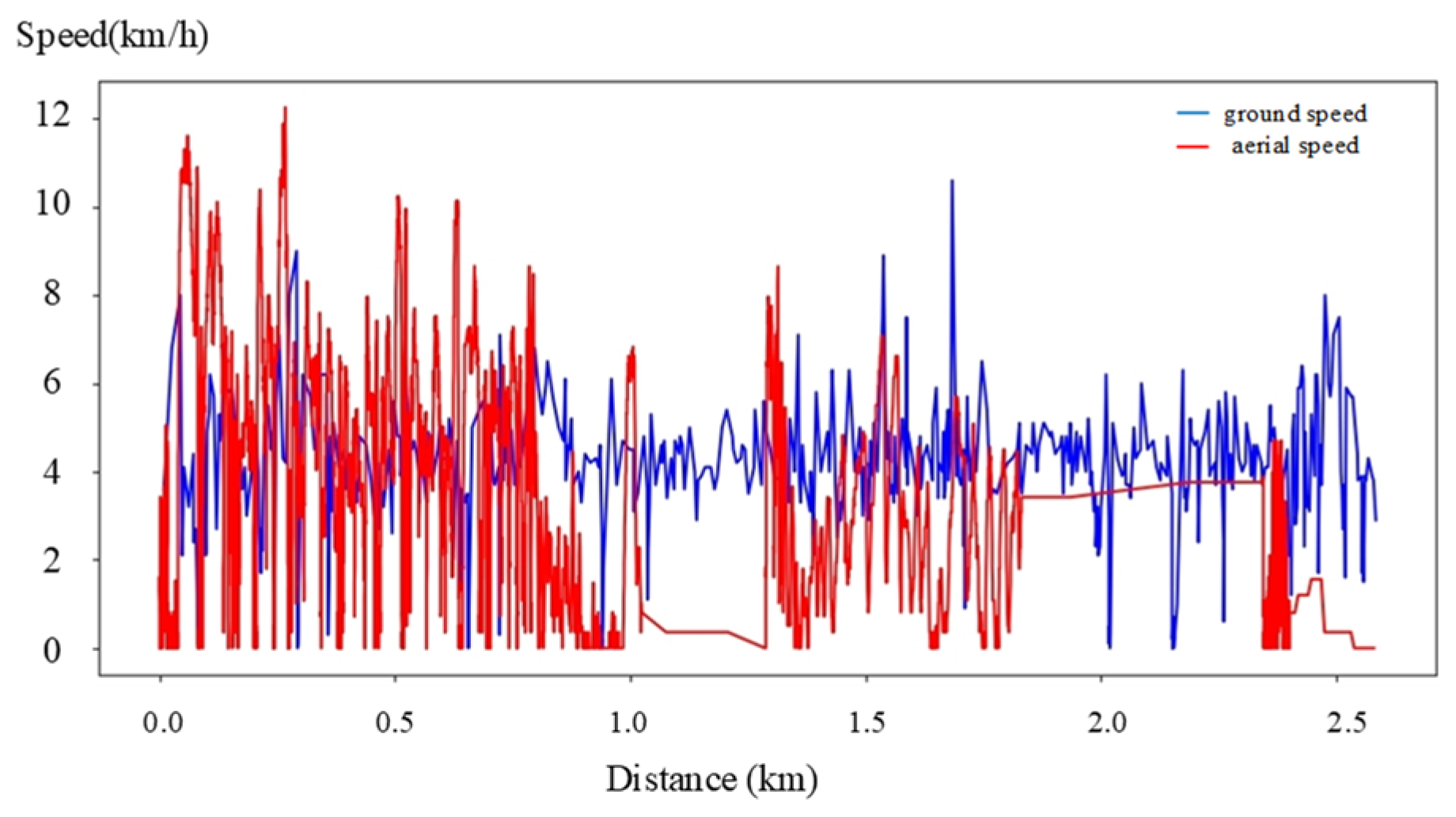
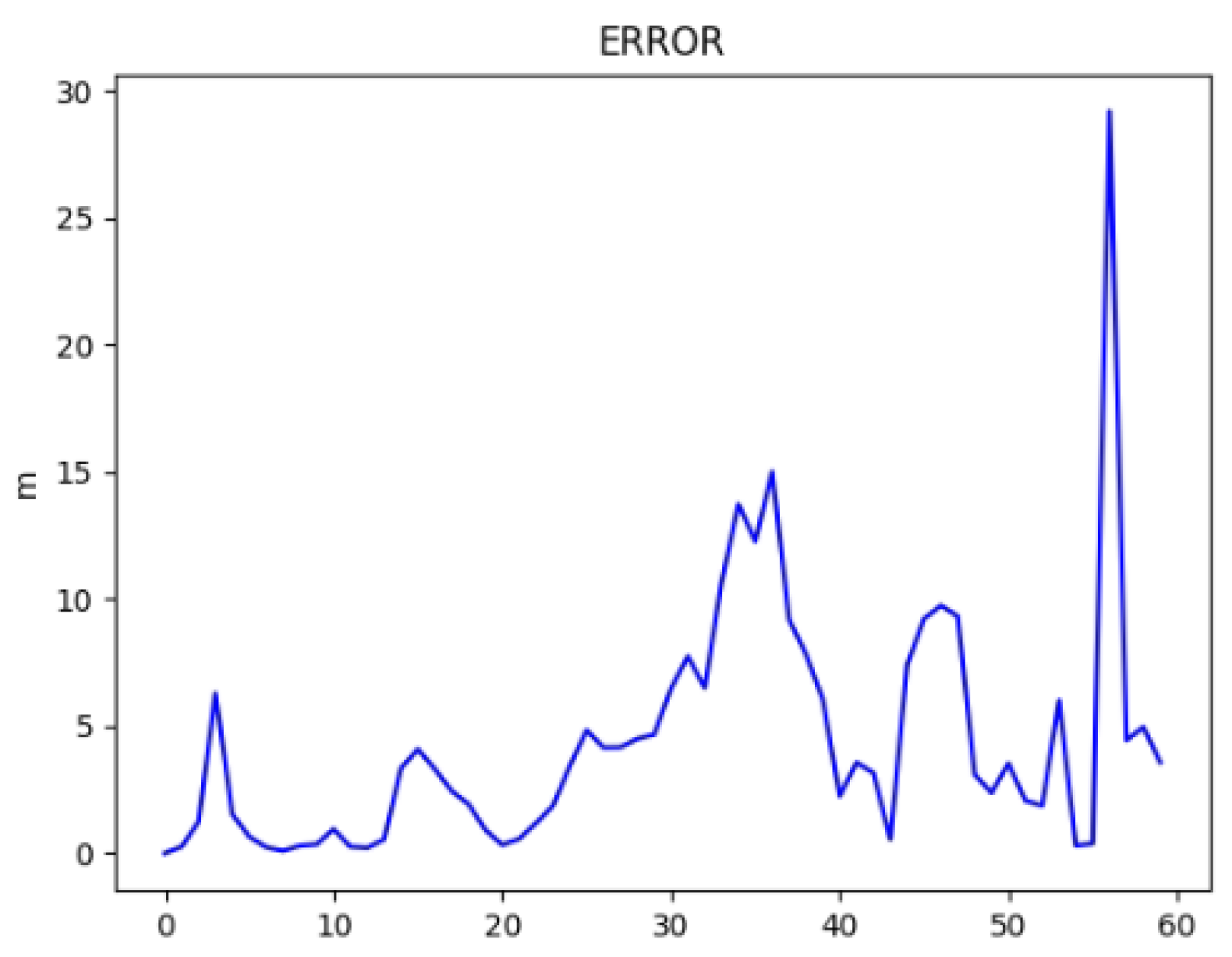
4.3. Heterogeneous Cooperation Experiments

To achieve heterogeneous cooperation between the UAV and ground vehicle, data such as pitch and yaw angles, altitude information from the UAV, and both ground and air speeds were utilized to calculate ground position coordinates. Figure 35 shows the altitude of the UAV while capturing aerial scenes, and Figure 36 illustrates the speeds of the UAV and target during scene capture. Figure 37 compares the aerial view coordinates with those calculated from ground-scene data. This integration of data enables the system to maintain a unified global coordinate system despite the challenges posed by speed variations and scene recognition errors.

As shown in Figure 38, the coordinates for the aerial experiments were recorded during the UAV’s flight. Figure 39 uses 60 key locations from Figure 38 to measure GPS positioning errors. These coordinates, calculated based on the positions obtained from both ground and aerial scenes, provide a comprehensive evaluation of localization performance. Positional errors caused by speed variations during the scene recognition process are reflected in the results. Additionally, the need to determine orientation at intersections introduces further complexity, as the ground camera rotates left and right to collect more feature information about the intersection. However, features such as store or road signs, often located on one side or the opposite side of the road (e.g., points 3, 6, 9, and 10 as shown in Figure 29), require the use of distant points as auxiliary positioning references in the GPS analysis process.

Obstructions in complex environments further complicate operations, as shown in Figure 14, where ground views are blocked by roadside trees. In such cases, the UAV compensates for missing depth data by leveraging its aerial map. The UAV’s overhead perspective identifies environmental features inaccessible to ground vehicles, providing critical supplementary data. However, the UAV’s localization accuracy can still be influenced by several factors:

• Speed Variations: fluctuations in UAV speed introduce delays in scene matching, leading to errors.
• Perspective Limitations: the UAV’s overhead view may result in mismatches in high-density or occluded areas.
• Camera Sensitivity: pitch and yaw angle sensitivity directly impact the accuracy of positioning results.

The experimental results indicate that when ground vehicles are obstructed and are unable to measure depth, the UAV can maintain overall positioning accuracy through its aerial perspective and flight data (Figure 39). However, the pitch angle sensitivity of the camera and factors such as air resistance and slope further affect the accuracy of the results. These challenges emphasize the need for the stabilization of UAV and camera movements to ensure consistent performance.

To address these limitations, the system employs an extended Kalman filter (EKF) for multi-source data fusion, integrating aerial and ground views into a unified global coordinate system. This approach stabilizes positioning results even when one data source is constrained. Additionally, stabilization algorithms were implemented to minimize pitch and yaw fluctuations caused by airflow and terrain irregularities. Future investigations should focus on refining these methods by accounting for air resistance and slopes, aiming to enhance the system’s overall efficiency and accuracy.

A sampled video demonstration of the real-world experiment can be viewed by accessing the following web link: https://youtu.be/ledLy4lgAuY (accessed on 7 January 2025).

5. Conclusions

This paper presents a GPS-denied positioning system that uses scene-image coordinates as an alternative to GPS signals, enabling effective operation even in environments where the GPS is unavailable or obstructed. By integrating aerial and ground-scene images, the system achieves a synergistic effect through the coordinated use of heterogeneous platforms, making it highly suitable for applications such as military missions, search and rescue operations, and commercial services. The ground-positioning system utilizes a feature identification model trained with deep learning to accurately recognize key scene features. By focusing solely on these features, the system accelerates the identification process while maintaining high accuracy and independence from the GPS. Positioning precision is further enhanced through a custom weight equation that refines coordinate determination.

In the aerial positioning component, managing a wide field of view presents a unique challenge. To address this, a camera gimbal tracking system locks onto ground targets, narrowing the coordinate range and stabilizing the system. Additionally, through coordinate conversion, if one unit temporarily loses recognition capabilities, the other can continue calculating the position, ensuring uninterrupted system operation and effective coordination between aerial and ground platforms. Unlike conventional systems that rely heavily on GPS signals, the proposed system provides a reliable solution for GPS-denied environments. It excels in critical situations where GPS signals may be blocked or lost, achieving practically acceptable positioning accuracy. Furthermore, the system’s heterogeneous coordination between aerial and ground units allows it to flexibly adapt to complex operational conditions. Real-world experiments have validated the applicability, reliability, and accuracy of this approach, demonstrating its potential as a robust alternative to traditional GPS-based positioning systems.

References

1. Radicioni, F.; Stoppini, A.; Tosi, G.; Marconi, L. Multi-constellation Network RTK for Automatic Guidance in Precision Agriculture. In Proceedings of the IEEE Workshop on Metrology for Agriculture and Forestry (MetroAgriFor), Perugia, Italy, 3–5 November 2022; pp. 260–265. [Google Scholar]
2. Feng, K.; Li, W.; Ge, S.; Pan, F. Packages delivery based on marker detection for UAVs. In Proceedings of the Chinese Control and Decision Conference (CCDC), Hefei, China, 22–24 August 2020; pp. 2094–2099. [Google Scholar]
3. Tippannavar, S.S.; Puneeth, K.M.; Yashwanth, S.D.; Madhu Sudanadhu, M.P.; Chandrashekar Murthy, B.N.; Prasad Vinay, M.S. SR2—Search and Rescue Robot for saving dangered civilians at Hazardous areas. In Proceedings of the International Conference on Disruptive Technologies for Multi-Disciplinary Research and Applications (CENTCON), Bengaluru, India, 22–24 December 2022; pp. 21–26. [Google Scholar]
4. Liu, K.; Lim, H.; Frazzoli, B.E.; Ji, H.; Lee, V.C.S. Improving Positioning Accuracy Using GPS Pseudorange Measurements for Cooperative Vehicular Localization. IEEE Trans. Veh. Technol. 2014, 63, 2544–2556. [Google Scholar] [CrossRef]
5. Deepika, M.G.; Arun, A. Analysis of INS Parameters and Error Reduction by Integrating GPS and INS Signals. In Proceedings of the International Conference on Design Innovations for 3Cs Compute Communicate Control (ICDI3C), Bangalore, India, 25–28 April 2018; pp. 18–23. [Google Scholar]
6. Cui, Y.-S. Performance Analysis of Deeply Integrated BDS/INS. In Proceedings of the Chinese Control and Decision Conference (CCDC), Shenyang, China, 9–11 June 2018; pp. 1916–1921. [Google Scholar]
7. Wu, Y.; Zhang, H.; Li, G.; Chen, P.; Hui, J.; Ning, P. Performance Analysis of Deeply Integrated GPS/BDS/INS. In Proceedings of the Chinese Control and Decision Conference (CCDC), Chongqing, China, 28–30 May 2017; pp. 81–85. [Google Scholar]
8. Chen, Z.; Qi, Y.; Zhong, S.; Feng, D.; Chen, Q.; Chen, H. SCL-SLAM: A Scan Context-enabled LiDAR SLAM Using Factor Graph-Based Optimization. In Proceedings of the IEEE International Conference on Unmanned Systems (ICUS), Guangzhou, China, 28–30 October 2022; pp. 1264–1269. [Google Scholar]
9. Tian, H.; Xia, L.; Mok, E. A Novel Method for Metropolitan-scale Wi-Fi Localization Based on Public Telephone Booths. In Proceedings of the IEEE/ION Position, Location and Navigation Symposium, Indian Wells, CA, USA, 3–6 May 2010; pp. 357–364. [Google Scholar]
10. Zamir, A.R.; Shah, M. Accurate Image Localization Based on Google Maps Street View. In Computer Vision—ECCV 2010. Lecture Notes in Computer Science; Daniilidis, K., Maragos, P., Paragios, N., Eds.; Springer: Berlin/Heidelberg, Germany, 2010. [Google Scholar]
11. Li, X.; He, H.; Huang, C.; Shi, Y. PCB Image Registration Based on Improved SURF Algorithm. In Proceedings of the International Conference on Image Processing, Computer Vision and Machine Learning (ICICML), Xi’an, China, 28–30 October 2022; pp. 76–79. [Google Scholar]
12. Fanqing, M.; Fucheng, Y. A tracking Algorithm Based on ORB. In Proceedings of the International Conference on Mechatronic Sciences, Electric Engineering and Computer (MEC), Shenyang, China, 20–22 December 2013; pp. 1187–1190. [Google Scholar]
13. Borman, R.I.; Harjolo, A. Improved ORB Algorithm Through Feature Point Optimization and Gaussian Pyramid. Int. J. Adv. Comput. Sci. Appl. 2024, 15, 268–275. [Google Scholar] [CrossRef]
14. Harris, C.; Stephens, M. A Combined Corner and Edge Detector. In Proceedings of the Alvey Vision Conference, Manchester, UK, 31 August–2 September 1988; pp. 147–151. [Google Scholar]
15. Perišić, A.; Perišić, I.; Perišić, B. Simulation-Based Engineering of Heterogeneous Collaborative Systems—A novel Conceptual Framework. Sustainability 2023, 15, 8804. [Google Scholar] [CrossRef]
16. Deng, H.; Huang, J.; Liu, Q.; Zhao, T.; Zhou, C.; Gao, J. A Distributed Collaborative Allocation Method of Reconnaissance and Strike Tasks for Heterogeneous UAVs. Drones 2023, 7, 138. [Google Scholar] [CrossRef]
17. Kwon, Y.H.; Jeon, J.W. Comparison of FPGA Implemented Sobel Edge Detector and Canny Edge Detector. In Proceedings of the IEEE International Conference on Consumer Electronics, Seoul, Republic of Korea, 26–28 April 2020; pp. 1–2. [Google Scholar]
18. Sudars, K.; Namatēvs, I.; Judvaitis, J.; Balašs, R.; Ņikuļins, A.; Peter, A.; Strautiņa, S.; Kaufmane, E.; Kalniņa, I. YOLOv5 Deep Neural Network for Quince and Raspberry Detection on RGB Images. In Proceedings of the Workshop on Microwave Theory and Techniques in Wireless Communications (MTTW), Riga, Latvia, 5–7 October 2022; pp. 19–22. [Google Scholar]
19. Yu, X.; Kuan, T.W.; Zhang, Y.; Yan, T. YOLO v5 for SDSB Distant Tiny Object Detection. In Proceedings of the International Conference on Orange Technology (ICOT), Shanghai, China, 15–16 September 2022; pp. 1–4. [Google Scholar]
20. Lestari, D.P.; Kosasih, R.; Handhika, T.; Murni; Sari, I.; Fahrurozi, A. Fire Hotspots Detection System on CCTV Videos Using You Only Look Once (YOLO) Method and Tiny YOLO Model for High Buildings Evacuation. In Proceedings of the International Conference of Computer and Informatics Engineering (ICCIE), Banyuwangi, Indonesia, 10–11 September 2019; pp. 87–92. [Google Scholar]
21. Yijing, W.; Yi, Y.; Xue-Fen, W.; Jian, C.; Xinyun, L. Fig Fruit Recognition Method Based on YOLO v4 Deep Learning. In Proceedings of the International Conference on Electrical Engineering/Electronics, Computer, Telecommunications and Information Technology (ECTI-CON), Chiang Mai, Thailand, 19–22 May 2021; pp. 303–306. [Google Scholar]
22. Fu, B.; Huang, L. Polygon Matching Using Centroid Distance Sequence in Polar Grid. In Proceedings of the IEEE International Conference on Computer and Communications (ICCC), Chengdu, China, 27–29 July 2016; pp. 733–736. [Google Scholar]
23. Wu, Y.; Ying, S.; Zheng, L. Size-to-depth: A new perspective for single image depth estimation. arXiv 2018, arXiv:1801.04461. [Google Scholar]
24. Liu, Y.; Sun, Z.; Wang, X.; Fan, Z.; Wang, X.; Zhang, L.; Fu, H.; Deng, F. VSG: Visual Servo Based Geolocalization for Long-Range Target in Outdoor Environment. IEEE Trans. Intell. Veh. 2024, 9, 4504–4517. [Google Scholar] [CrossRef]
25. Woodall, W.; Liebhardt, M.; Stonier, D.; Binney, J. ROS Topics: Capabilities [ROS Topics]. IEEE Robot. Autom. Mag. 2014, 21, 14–15. [Google Scholar] [CrossRef]
Figure 1. SIFT extracts feature points from an image.
Aerospace 12 00039 g001
Figure 2. SIFT generates descriptors for features. The original input image shows the entrance gate.
Aerospace 12 00039 g002
Figure 3. SURF extracts feature points from an image. The left panel illustrates the utilization of integral images and box filters to facilitate efficient feature detection across multiple scales. The central image depicts the process of feature detection across various layers within the scale-space pyramid. The right panel exemplifies the localization of key points at different scales.
Aerospace 12 00039 g003
Figure 4. Descriptor gradient orientation of SURF. The circle is an area surrounding a keypoint as defined by regions for computing the dominant orientation. The red dot shows the pixel samples that were used for calculating detectors orientation. The light gray shaded area indicates the current sector being analyzed. The blue arrow indicates the direction of the dominant orientation which corresponds to the sum of Haar wavelet responses in the sector. This implies rotation invariance, because the descriptor is aligned with the main orientation.
Aerospace 12 00039 g004
Figure 5. ORB feature matching. The colored lines indicate the matched feature points between the two images. Each line represents a correspondence between keypoints in the images, with different colors distinguishing various matching pairs.
Aerospace 12 00039 g005
Figure 6. Images and labels for the road signs and shop signs in the training set.
Aerospace 12 00039 g006
Figure 7. Sampled images and labels for the feature ground in the training set.
Aerospace 12 00039 g007
Figure 8. F1-score of the training model.
Aerospace 12 00039 g008
Figure 9. These labeled features, including shop signs, road signs, and text-based features, were arranged and stored in the database for subsequent detection and matching processes. The numbering in the figure represents the sequence of the selected features.
Aerospace 12 00039 g009
Figure 10. Simulated GPS coordinates for the paired images.
Aerospace 12 00039 g010
Figure 11. Calculation of depth using the depth camera on the x-axis.
Aerospace 12 00039 g011
Figure 12. Actual depth map detected by the depth camera.
Aerospace 12 00039 g012
Figure 13. The operational flow of EKF fusion.
Aerospace 12 00039 g013
Figure 14. The ground view obstructed by roadside trees.
Aerospace 12 00039 g014
Figure 15. A sampled aerial image containing distinct features with different coordinates.
Aerospace 12 00039 g015
Figure 16. Positional relationship between the screen center and the target.
Aerospace 12 00039 g016
Figure 17. Diagram of the world and onboard IMU coordinate frames.
Aerospace 12 00039 g017
Figure 18. The camera gimbal’s structure.
Aerospace 12 00039 g018
Figure 19. Camera gimbal’s coordinate conversion.
Aerospace 12 00039 g019
Figure 20. Illustration of the FOV.
Aerospace 12 00039 g020
Figure 21. Relationship between target image and global coordinate system.
Aerospace 12 00039 g021
Figure 22. The geometric relationship between the UAV and the target person.
Aerospace 12 00039 g022
Figure 23. Relation diagram between topic and node.
Aerospace 12 00039 g023
Figure 24. Flowchart of the system operation.
Aerospace 12 00039 g024
Figure 25. Operating image of the positioning system for ground.
Aerospace 12 00039 g025
Figure 26. Walking speed while capturing the ground scene.
Aerospace 12 00039 g026
Figure 27. Depth values between the features and ground camera.
Aerospace 12 00039 g027
Figure 28. Coordinates for ground-view experimental results and error analysis. The numbers in the figure correspond to specific locations where images were captured during the ground experiment.
Aerospace 12 00039 g028
Figure 29. Image of the positioning system in operation for aerial scene capture.
Aerospace 12 00039 g029
Figure 30. Depth values between the features and the aerial camera.
Aerospace 12 00039 g030
Figure 31. Flight speed while capturing the aerial scene.
Aerospace 12 00039 g031
Figure 32. Pitch and yaw angle of the UAV camera.
Aerospace 12 00039 g032
Figure 33. Coordinates of the aerial-view experiment.
Aerospace 12 00039 g033
Figure 34. Errors between ground image coordinates and GPS coordinates.
Aerospace 12 00039 g034
Figure 35. The UAV altitude while capturing the aerial scene.
Aerospace 12 00039 g035
Figure 36. Speed of the UAV and ground target while capturing the aerial scene.
Aerospace 12 00039 g036
Figure 37. Comparison of the ground coordinates to the aerial coordinates.
Aerospace 12 00039 g037
Figure 38. Comparison of the aerial coordinates to the ground coordinates.
Aerospace 12 00039 g038
Figure 39. Errors between aerial image coordinates and GPS coordinates.
Aerospace 12 00039 g039