Article

A Neural Network with Physical Mechanism for Predicting Airport Aviation Noise

1
College of Civil Aviation, Nanjing University of Aeronautics and Astronautics, Nanjing 210016, China
2
College of Materials Science and Technology, Nanjing University of Aeronautics and Astronautics, Nanjing 210016, China
*
Author to whom correspondence should be addressed.
Aerospace 2024, 11(9), 747; https://doi.org/10.3390/aerospace11090747
Submission received: 20 July 2024 / Revised: 10 September 2024 / Accepted: 11 September 2024 / Published: 12 September 2024
(This article belongs to the Section Air Traffic and Transportation)

Abstract

:
Airport noise prediction models are divided into physics-guided methods and data-driven methods. The prediction results of physics-guided methods are relatively stable, but their overall prediction accuracy is lower than that of data-driven methods. However, machine learning methods have a relatively high prediction accuracy, but their prediction stability is inferior to physics-guided methods. Therefore, this article integrates the ECAC model, driven by aerodynamics and acoustics principles under the framework of deep neural networks, and establishes a physically guided neural network noise prediction model. This model inherits the stability of physics-guided methods and the high accuracy of data-driven methods. The proposed model outperformed physics-driven and data-driven models regarding prediction accuracy and generalization ability, achieving an average absolute error of 0.98 dBA in predicting the sound exposure level. This success was due to the fusion of physics-based principles with data-driven approaches, providing a more comprehensive understanding of aviation noise prediction.

1. Introduction

With the development of airport economics, noise pollution around airports has become a significant problem that restricts the development of the airport economy. It is urgently needed to carry out daily noise monitoring to obtain the distribution of airport noise and formulate effective noise control measures. Due to cost constraints, deploying high-density noise monitoring equipment around an airport perimeter is impractical. A feasible solution is to deploy a relatively small number of receivers at airports using automatic dependent surveillance-broadcast (ADS-B) to capture real-time flight operations [1,2,3]. The noise impact generated by each aircraft can be predicted in real-time from the collected trajectory data [4].
Classical physics-based and data-driven methods have been successfully applied to airport noise prediction [5]. However, the physics-driven approach is best suited for predicting cumulative airport noise in the long term, such as annual, monthly, and daily cumulative event noise. This approach has limited accuracy for single-event noise prediction, with an error of 3–4 dBA for the maximum A-weighted sound level [6,7]. Data-driven machine learning models require a large amount of data for training and have high input data quality requirements. These data requirements limit many researchers, who resort to using simulation data derived from physics-driven models rather than real aviation noise datasets [8,9]. To handle complex nonlinear systems like aviation noise, machine learning models using real-world datasets become increasingly complex and difficult to interpret [10].
In some cases, machine learning models outperform classical physics-based models [11]. However, machine learning models have poor generalization capabilities, due to the lack of clear physical meaning [12,13]. When there is insufficient reliable training data, the prediction accuracy of machine learning models can be significantly reduced [14]. Physics-based models, such as the best-practice and scientific predictions, are built on physical-based methods and theoretical analyses that are not dependent on data quality. Noise models based on physical processes require complex theoretical assumptions and many parameter calibration adjustments. Their advantage is that they can present the underlying mechanisms of aviation noise, and their prediction results are scientifically interpretable [15,16,17]. The disadvantage of physics-based models is that they require complex theoretical assumptions and have difficulty capturing the uncertainty in data [18].
Data-driven machine learning models can be challenging to apply to untrained scenarios because they often fail to capture the complex relationships in the data, mainly when the data quality is poor [19,20,21]. To address the limitations of data-driven models, some researchers have investigated methods for incorporating prior knowledge from physics-driven models into machine learning models. Data-driven models that include physical knowledge can be divided into two types. One approach is hybrid physics neural networks (HPNN), which use the physical model output as the input feature variable. Murphy, for instance, constructed feature variables based on a sparse transfer matrix physical model as input to a neural network for predicting chemical features [22]. Changdar used physical-model-derived input features such as density, volume fraction, size, the temperature of nanoparticles, the base fluid’s viscosity, and the nanofluid’s simulated viscosity to build a deep neural network model for predicting the viscosity of nanofluids [23].
Another method for incorporating physical knowledge into data-driven models is using physics-driven models to build loss functions for neural network models, guiding them toward training in a direction consistent with physical criteria. Such models that include physical knowledge in training neural networks are called physics-guided neural networks (PGNN), also known as physical information-based neural networks (PINN). Physics-guided neural network modeling is a technique for embedding knowledge of physical processes into machine learning models. It combines the strengths of physical knowledge and machine learning models to improve the accuracy and reliability of the model. A PGNN model accurately captures the uncertainty in the prediction process, resulting in a more comprehensive and robust performance. The effectiveness of PGNN models in various fields has recently been acknowledged. For instance, Karpatne proposed a physics-guided neural network model for predicting lake temperature [13,24]. At the same time, Uzun developed a physics-guided deep neural network model for predicting the fuel consumption of an aircraft and established a loss function for fuel consumption based on a physical approach, to guide the optimization direction of the deep learning model [25]. PGNN models have also shown excellent performance in turbulence modeling [26], Earth systems [27], materials discovery [28], quantum chemistry [29], biosciences [30], and other fields.
In order to effectively overcome the limitations of physically driven and purely data-driven models in solving the single-event noise prediction problem at airports, a new physics guided neural network (PGNN) model is introduced in this chapter. The framework skillfully fuses the specialized physics knowledge of the European Civil Aviation Conference (ECAC) model constructed based on aerodynamic and acoustic principles with the powerful data-driven capabilities of deep neural networks (HPNN). Through this fusion strategy, we construct a physics-guided deep neural network model designed to predict airport noise. In this model, the physical principles not only serve as the theoretical basis, but also directly guide the training process of the deep neural network to ensure that the prediction results follow the physical laws as much as possible, which significantly improves the robustness and reliability of the model. This physical steering mechanism not only optimizes the learning path of the network, but also guides the network to correct the ECAC model through input features. While this correction improves the predictive performance of the model, it also introduces a new “black box” and thus requires further attention with respect to its impact on physical consistency and potential opacity. In the end, we realized a highly accurate prediction model that can accurately monitor and predict the noise level in the surrounding area of an airport, which provides strong technical support and a decision-making basis for environmental protection, urban planning, and aviation noise management.
This paper is organized as follows: Section 2 introduces a detailed description of the PGNN models for aviation noise prediction. The testing results of different models are presented and discussed in Section 3, and the conclusions are given in Section 4.

2. Methodology

This paper explores a fusion model of physics-driven and machine-learning models. It introduces the optimal application and combination of physical drivers and machine learning methods in aircraft noise research. The objective was to identify potential patterns in single-event noise from a large volume of historical trajectory data and to predict online flight noise using the established fusion model. In the single-event noise prediction problem, the model predicts the impact of a flight’s noise on a ground noise-sensitive point in real time by analyzing the track passage characteristics that produce noise impacts at the ground noise-sensitive point and considering the influence of meteorological factors on noise propagation [31,32]. Figure 1 illustrates the general framework of the physics-guided neural-network-based aircraft noise prediction model developed in this paper. The model combines the advantages of a physics-driven ECAC model and a data-driven machine learning model to construct additional physical parameters that represent aircraft performance characteristics with the physical model. The loss function of the machine learning model is built using a physical method, to guide the neural network training, ultimately realizing real-time prediction at airports.

2.1. ECAC Model

The ECAC noise model is a best-practice segmentation model proposed by the European Civil Aviation Conference for predicting aviation noise around airports. The model is a unified noise modeling approach established throughout Europe [33] and validated by the DOC 9911 document correlation proposed by the International Civil Aviation Organization (ICAO) [34,35]. The ECAC model is based on segmented trajectories for analysis and relies on noise–power–distance (NPD) curves for noise calculation and the final output of predicted noise [36,37]. This paper uses the ECAC model as a physically driven model for physically guided machine learning.
The noise calculation of the ECAC model follows the following assumptions.
  • The propagation of aviation noise remains isotropic.
  • The aircraft engine power, climb or descent angle, flap settings, and other flight states remain unchanged in each segmented track, i.e., the flight state is updated once per track segment.
  • The ground is a constant single medium with negligible noise absorption.
The ECAC model can calculate noise sound pressure levels by superimposing the segment noise impact of individual flight events. Each flight event trajectory is divided into a series of 3D trajectory segments. Each segment is defined by the geometric coordinates of its endpoints, velocity, and engine thrust settings, and further categorized as either a ground track or a flight profile. Combining a 2D horizontal profile track with a flight profile that represents the aircraft’s flight along the ground track, a series of 3D track segments are created. The ground track describes the aircraft’s position on the ground projection, while the flight profile trajectory describes the aircraft’s variation in altitude, velocity, and thrust settings. Together, they form a profile that represents the aircraft’s flight status, including the slope profile, velocity profile, and engine thrust profile, among others [38,39]. The slope distance of the ground is relative to the aircraft, and the angle of noise generation is determined by the location of noise-sensitive points on the ground and the spatial orientation of the aircraft, while the meteorological conditions around the airport determine the propagation characteristics of the noise. By analyzing the noise impact of each segment of the flight trajectory, the ECAC model can calculate the noise level at any given point around the airport.
The exposure level of single-event noise is determined by calculating the physical component of the exposure level of each segment trajectory and then summing the logarithms of the noise of all segments. This calculation can be expressed as follows:
Y p h y = 10 * lg ( 10 Y p h y , s e g / 10 )
For each track segment, it is necessary to calculate the slope distance between the location of the noise observation point and the flight thrust of the track point. Once completed, the NPD data from the identified model should be corrected for atmospheric factors and interpolated to determine the aviation noise baseline value. The base noise is then corrected for the calculation to ensure that the noise calculation conforms to the physical criteria for noise propagation. Aviation noise is calculated as follows:
Y p h y , s e g = L re ( P , d ) + Δ v + E E n g ( φ ) Λ ( β , l ) + Δ F
where L re ( P , d ) indicates NPD data corrected by SAE-ARP-5534 atmospheric factors. Atmospheric factor correction removes the average atmospheric attenuation correction from the original NPD data in the Aircraft Noise and Performance (ANP) database [40]. Then, it applies a new atmospheric attenuation correction to obtain a new NPD curve corresponding to a specific temperature, atmospheric pressure, and relative humidity.
Δ v indicates duration correction. Duration correction is a method used to account for the effect of aircraft speed on the duration of a noise event. The underlying theoretical assumption is that, all other things being equal, the duration and the received noise energy are inversely proportional to the aircraft speed. Therefore, if the actual speed of the aircraft differs from the reference speed provided by the ANP database, duration correction is needed to estimate the duration and noise level of the event accurately.
E E n g ( φ ) indicates the installation effect. The noise generation mechanism of aircraft during operation is highly complex and involves multiple noise sources [41]. The structure of the aircraft, its flight attitude, and the engine installation position can all impact the noise emissions. In addition, noise shielding, refraction, and reflection caused by the engine and airframe can result in directional aviation noise [42]. Figure 2 illustrates the angular parameters of the aircraft observed by the ground-based observation points. The parameters include the elevation angle β , pitch angle φ , and inclination angle ε , which are the angles between the observation point and the aircraft’s position. Lateral distance indicates the vertical distance from the position of the ground observation point to the aircraft’s ground track.
Λ ( β , l ) indicates lateral attenuation. The noise level measured by an observer on the side of a flight track segment is usually lower than the noise pressure level measured directly beneath the track at the same distance. This is because sound waves can be absorbed by surfaces and refracted or scattered by wind and meteorological conditions, resulting in lower noise levels being measured by the side observer due to a greater probability of refraction [43]. For this reason, the sound level at an observer some lateral distance from the track is different from the value listed in the NPD database. This correction is important for the low-angle noise propagation to the ground.
Δ F indicates finite segment correction (noise fraction). The sound exposure level values presented in the ANP are calculated based on the assumption of an infinitely long flight segment. In practice, the length of the noise-generating track segment is finite, meaning that the energy received at the observation point represents only a fraction of the total noise generated during the flight.

2.2. Neural Networks

2.2.1. Input Features

Neural networks based on machine learning use multiple hidden layers to model nonlinear systems that involve multiple feature vector inputs. Such networks’ output results depend on the input of the feature vectors, making it important to select appropriate input variables [44,45]. The model input features for this study include raw trajectory data, meteorological data, and physical features constructed using the ECAC method, such as engine thrust and aircraft weight. The sound exposure level generated by each flight operation is used as the prediction label for the model.
  • Flight trajectory
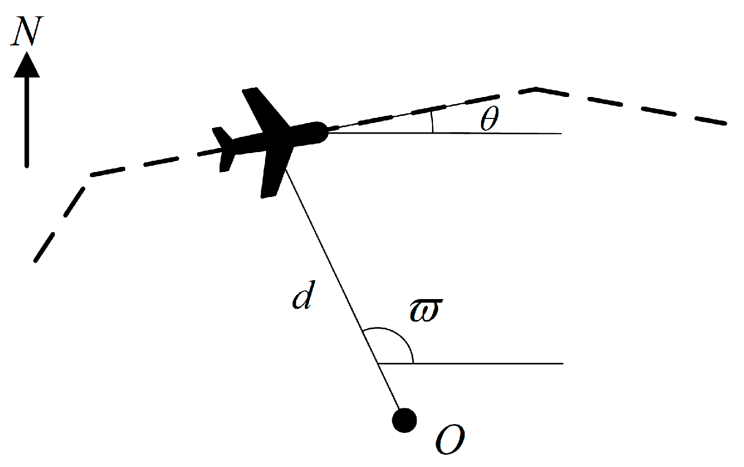
The basic attributes of the closest point in the track segment constructed from the ADS-B data include slope distance, speed, azimuth, heading, approach, and departure type. The slope distance d , azimuth ω, and heading θ are visually depicted in Figure 3.
For the accurate prediction of single-event noise, it is crucial to select track segments that significantly impact ground noise-sensitive points as inputs to the model. Typically, the noise generated by an aircraft 3 NM away from the ground observer’s position does not exceed the ambient background noise [46]. In this paper, we selected the track segment within 3 NM from the ground observer’s position as the model input segment. We defined the moments when the aircraft enters and exits the segment as t 1 and t 2 , respectively.
As shown in Figure 4a, the trajectory between periods t 1 t 2 contains most of the aircraft’s noise impact on the ground observation point. The track segment S 1 S 2 in Figure 4b comprises the track points from the period t 1 t 2 shown in Figure 4a.
The characteristic parameters of the segment S 1 S 2 are defined by the position S P , which is closest to the ground observation point O in the segment. Specifically, the speed, lateral distance, azimuth, and heading of the segment are defined as the values of the aircraft at the moment of position S P .
2.
Meteorological data
In the process of propagation, the energy of sound is gradually absorbed by the air medium, resulting in energy loss. The loss of sound energy propagation is related to environmental factors such as temperature, atmospheric pressure, humidity, etc. When calculating cumulative event noise with a year–month–day approach, the impact of meteorological factors is typically smaller [47]. Nevertheless, the impact of atmospheric factors is notably significant in modeling single-event noise. Meteorological factors, such as temperature, atmospheric pressure, relative humidity, and wind speed, which are known to affect noise, must be considered in the modeling process [48,49]. In our study, all meteorological data are detected by the airport’s meteorological radar, including temperature, atmospheric pressure, and relative humidity every minute, and wind speed and direction every two minutes.
3.
Engine thrust and aircraft weight
Two derived physical properties, engine thrust and aircraft weight, are included as additional inputs to the model [50]. These derived features are constructed based on the aerodynamic characteristics of different aircraft types, the operating conditions of the aircraft, and the overall characteristics of the flight track segment.
One of the primary causes of aviation noise is the sound produced by aircraft engines. In a physics-based noise prediction model, two key parameters used to estimate the noise generated by aircraft are the slant distance and the engine thrust. Therefore, accurately calculating engine thrust is critical to accurately predicting aviation noise levels. However, radar data alone cannot provide information on thrust setting, so estimates must be based on the available engine performance and trajectory data.
Different aircraft follow different operating procedures during approach and departure, resulting in significant variations in flight patterns and engine operating conditions. As a result, calculating engine thrust for approach and departure flights must be considered separately. The aircraft trajectory can be determined using the ANP database to calculate the net thrust correction for departure flights. The calculation process is as follows:
P = E + F * V C A S + G A * h + G B * h 2 + H * T
where P is the modified net thrust per engine of the aircraft; h is the altitude of the aircraft; and E , F , G A , G B , and H are the engine thrust-related constants provided for the ANP database, which are different for different operating modes (e.g., Normal, MaxTakeoff, MaxClimb) and for different operating temperatures (normal, high), respectively.
The corrected net thrust for the approach flight is calculated using the aircraft weight, drag-to-lift ratio, angle of ascent/descent, and ground speed acceleration:
P = W R a cos γ + sin γ + a / g n δ
a = ( V 2 / cos γ ) 2 ( V 1 / cos γ ) 2 2 Δ s / cos γ
where W is the aircraft weight; R a is the ratio of the aircraft drag coefficient for a given flap setting to its lift coefficient; γ is the descent angle; n is the number of engines; V1 and V 2 are the groundspeed at the beginning and end of the track segment; and Δ s is the ground projection distance of the track segment.
Another characteristic related to noise that needs to be considered is aircraft weight. Estimating aircraft weight depends on the type of flight and the approach and departure methods. For arriving aircraft, the current weight is estimated as 90% of the maximum gross landing weight (MGLW) specified in the ANP database. Estimating the weight of departing aircraft is a bit more complex because it depends heavily on the amount of fuel carried by aircraft, which is related to the distance between the departing and destination airports. In this paper, an aircraft’s take-off weight (TOW) is estimated based on the great circle distance between the departure airport and the destination airport. Using a B772 aircraft as an example, Table 1 presents the conversion of estimated aircraft weight from the great circle distance between the departure and landing airports. As the distance to the destination airport increases, the B772 aircraft carries a higher fuel load and becomes heavier.
The complete list of input features is as follows:
  • Slant distance d and azimuth angle ω . Aircraft position relative to a ground observer.
  • Ground-speed v and heading of the aircraft θ .
  • Arrival or departure. Indication of the operation type of the flight
  • Airport temperature, humidity, and atmospheric pressure at the nearest 1 min time
  • Wind speed and direction at the nearest 2 min time
  • Engine thrust and aircraft weight constructed using ECAC model

2.2.2. Neural Network

  • DNN model
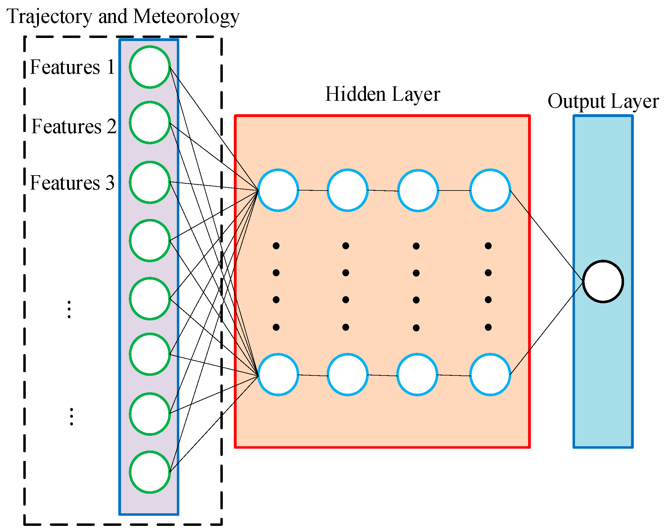
The underlying data-driven model employed in this paper is the DNN neural network, as shown in Figure 5. DNNs are typical fully connected layer neural network models, generally consisting of many serially connected layers, including an input layer, hidden layers, and an output layer. This network structure has been shown to capture complex nonlinear input–output relationships through gradient-based optimization [51,52]. The structure of a network with M implicit layers can be expressed as follows:
g 1 = S ( W 1 X + b 1 ) g 2 = S ( W 2 g 1 + b 2 )    g M = S ( W M g M 1 + b M ) G = W M + 1 g M + b M
where W i and b i denote the weights and deviations of the hidden layer, respectively; g i denotes the output of the hidden layer; and G denotes the final output of the model. The loss function of the neural network calculates the mean square error between the output value of the model and the true value, which is expressed as follows:
L o s s D N N = 1 N i = 1 N | h ( W D N N , b D N N ; X ) G |
where W D N N and b D N N denote the network parameters of the model during training. The training is terminated when the error reaches a level that satisfies a certain accuracy.
2.
HPNN model
The HPNN model aims to enhance the predictive capabilities of traditional deep learning models by integrating domain-specific physical principles. It utilizes a DNN as the core data-driven component for handling regression tasks. The structure of the HPNN model is shown in Figure 6. What sets the HPNN model apart is its innovative combination of data-driven and physics-driven approaches, allowing it to capture both empirical patterns and theoretical knowledge from the data.
The input to the HPNN model is carefully designed and comprises two distinct but complementary parts. The first part of the input is identical to that used in the DNN. It includes basic trajectory features, as well as meteorological features. These features represent empirical data collected from real-world observations and are crucial for capturing patterns that the model can directly learn from. The second part of the input comes from the output of the ECAC model. The ECAC model integrates aerodynamic and acoustic principles to simulate the physical phenomena relevant to the task at hand. By incorporating these outputs, the HPNN model benefits from the theoretical insights provided by physics-based simulations, which are often difficult to obtain through data-driven methods alone.
These two parts are not handled in isolation. Instead, the HPNN model is designed to seamlessly integrate them, allowing the physics-driven input to enhance and guide the learning process of the data-driven model. This combination enables the HPNN to leverage the strengths of both approaches simultaneously. By integrating physical principles, the model can achieve higher predictive accuracy, particularly in cases where data are sparse or noisy.
Although the HPNN model introduces physics-driven feature inputs, its loss function remains consistent with that of the DNN model, measuring the model’s prediction performance by calculating the mean squared error (MSE) between the predicted values and the true values. This is because the goal of the HPNN is still to minimize the error between the predicted and true values, and the MSE provides a simple and effective way to assess this error, which is expressed as follows:
L o s s H P N N = 1 N i = 1 N | h ( W H P N N , b H P N N ; X ) G |
where W H P N N and b H P N N denote the network parameters of the model during training. The training is terminated when the error reaches a level that satisfies a certain accuracy.
3.
PGNN model
The PGNN (physics-guided neural network) model is a further improvement on the DNN model and the HPNN model. Compared with the traditional DNN and HPNN models, the PGNN embeds physical constraints into the loss function to guide model training, so that the model output is consistent with the physical laws during the training process. The physics-driven loss function is calculated as follows:
P G L o s s = l o s s ( Y , Y p r e ) + η l o s s ( Y p r e , Y p h y )
where the l o s s ( Y ,   Y p r e ) is the empirical error between the real value of noise monitoring and the output value of PGNN; and l o s s ( Y p r e ,   Y p h y ) refers to the physical error, also known as physical inconsistency, between the PGNN output and the ECAC model output. This error is used to maintain consistency between the model predictions and physical laws and to ensure the accuracy of the model. The empirical and physical errors are weighted to improve the model’s final prediction performance. The performance of data-driven deep learning models is closely related to the hyperparameter settings. In this study, the weightings of the empirical and physical errors are set to 1 and η , where η is the physical error weight hyperparameter. This choice helps to reduce the number of hyperparameters needed for the model, simplifying the optimization process.
The physical component of the exposed sound level Yphy,seg for each segmental track can be calculated by Equation (10). Therefore, the physical loss of aviation noise for the k flight segments can be expressed as follows:
l o s s ( Y p r e , Y p h y ) = 1 N i = 1 N | h ( σ ; X ) 10 * lg ( i = 1 k 10 Y p h y , s e g / 10 ) |
Therefore, the loss function of the PGNN-based single-event noise prediction model for airports is as follows:
P G L o s s = 1 N i = 1 N | h ( σ ; X ) G | + η 1 N i = 1 N | h ( σ ; X ) 10 * lg ( i = 1 k 10 Y p h y , s e g / 10 ) |

2.3. Implementation

The ECAC model is a physical model, while the DNN model is a basic neural network model. The HPNN model incorporates physical guidance on the basis of a DNN to enhance the physical consistency of the model. The PGNN model, on the basis of the DNN and HPNN models, further improves the expressiveness and accuracy of the model by introducing physical guidance in the loss function. The algorithms of those models used in this paper are shown in Algorithms 1–5.
Algorithm 1: ECAC-based single-event noise prediction algorithms
Input:
1. Standardized trajectory V t r a j e c t o r y , includes monitoring time, longitude, latitude, altitude, ground speed, flight number and heading
2. Meteorological feature datasets V m e t e o includes temperature, atmospheric pressure, relative humidity, wind speed and direction
3. ANP Database
Process:
1. Determine the coordinates of ground monitoring observation points
2. ( E i , F i , G A , i , G B , i , H i , N P D i ) Match( T R i ) // Match NPD curves
3. n e w _ N P D i N P D i // Update to correct the NPD curve
4. for i 1 to N do
   P s e g , i T R i = { x 1 , x 2 , , x k } , i [ 1 , N ] ; // Calculate engine thrust
   W i T R i = { x 1 , x 2 , , x k } , i [ 1 , N ] ; // Calculate aircraft weight
   Y p h y T R i = { x 1 , x 2 , , x k } , i [ 1 , N ] ; // Calculate Sound Exposure Level using ECAC
end for
Output:
ECAC model-calculated single-event noise sound exposure levels Y p h y
Algorithm 2: Implementation steps of DNN algorithm
Input:
1. Standardized trajectory V t r a j e c t o r y , includes monitoring time, longitude, latitude, altitude, ground speed, flight number and heading
2. Meteorological feature datasets V m e t e o includes temperature, atmospheric pressure, relative humidity, wind speed and direction
3. Number of hidden layers L
4. Number of neurons in each hidden layer N
Loss function construction:
The loss function of the DNN is to calculate the mean square error between the output value of the model and the true value L o s s D N N
Output:
DNN model-calculated single-event noise sound exposure levels Y D N N
Algorithm 3: Implementation steps of HPNN algorithm
Input:
1. Standardized trajectory V t r a j e c t o r y , includes monitoring time, longitude, latitude, altitude, ground speed, flight number and heading
2. Meteorological feature datasets V m e t e o includes temperature, atmospheric pressure, relative humidity, wind speed and direction
3. Number of hidden layers L
4. Number of neurons in each hidden layer N
5. ECAC model-calculated single-event noise sound exposure levels Y p h y
Loss function construction:
The loss function of HPNN is the same as that of DNN, which calculates the mean square error between the model output value and the true value L o s s H P N N .
Output:
HPNN model-calculated single-event noise sound exposure levels Y H P N N
Algorithm 4: Implementation steps of PGNN algorithm
Input:
1. Standardized trajectory V t r a j e c t o r y , includes monitoring time, longitude, latitude, altitude, ground speed, flight number and heading
2. Meteorological feature datasets V m e t e o includes temperature, atmospheric pressure, relative humidity, wind speed and direction
3. Number of hidden layers L
4. Number of neurons in each hidden layer N
5. ECAC model-calculated single-event noise sound exposure levels Y p h y
6. Physical constraint weight η
Loss function construction:
Add physical condition constraints to the loss function of the original HPNN model to guide the model to optimize in the direction of physical consistency and obtain the loss function P G L o s s .
Output:
PGNN model-calculated single-event noise sound exposure levels L S E L
Algorithm 5: The training process of DNN, HPNN, and PGNN
1. Back propagation optimization is performed with the goal of minimizing the loss function construction. The Adam optimizer is used to update the model weight parameters and continuously adjust the parameters to optimize the model. By using a K-fold cross-validation method (specifically set to k = 5), we iteratively train the model using the training set data. In each round of cross-validation, the model is trained on a training subset and evaluated on a validation subset.
2. If the error metrics obtained after cross-validation meet the expected performance criteria, this indicates that the model training is complete and meets the predefined accuracy requirements. Conversely, if the error does not meet expectations, we will repeat the training and optimization steps of the model until we obtain results that satisfy the desired training model performance.

3. Validation

3.1. Data Description

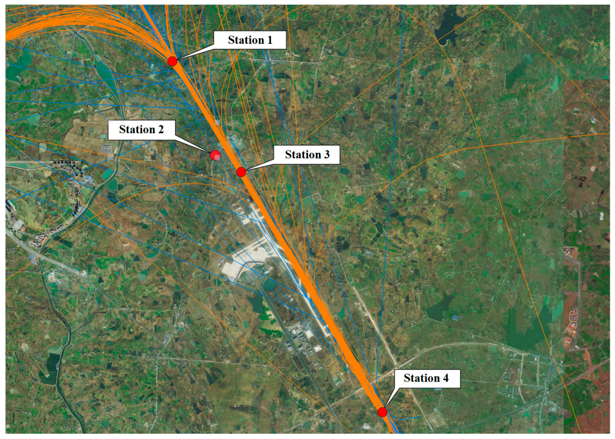
The data for this study come from Hefei Xinqiao International Airport (HFE), which is located in Shushan District, Hefei City, Anhui Province, China. The data used for this study include aircraft noise monitoring data spanning from July 2022 to October 2022, ADS-B data, meteorological data, and aircraft performance data sourced from the ANP database. The ADSB attributes are shown in the Table 2, and the meteorological attributes include temperature, atmospheric pressure, relative humidity, and wind speed and direction. The noise model used in this study is based on archived datasets from four noise monitoring stations, as shown in Figure 7. The dataset contains a total of 3195 flight information records, of which the data from monitoring point 2 were divided in a ratio of 80% for training and 20% for testing. Meanwhile, the data from monitoring points 1, 3, and 4 were dedicated to testing the generalization performance of the model. The noise monitoring equipment continuously and uninterruptedly receives noise information every second. In contrast, the ADS-B receiver receives signals from individual aircraft in real-time. ADS-B signals from multiple flights received at the same time node are analyzed to select the closest aircraft to the ground monitoring station. The aircraft position information is calculated based on the last received real-time position per second of the ADS-B signal for that flight. This process is repeated for each second of the flight’s trajectory.
In response to the challenge of missing values in the data, this study innovatively used piecewise cubic Hermite interpolation polynomial (PCHIP) technology to ensure the integrity and continuity of the data. In addition, to further refine the data quality, the study also implemented regularized reconstruction technology to effectively identify and remove abnormal data points, smooth the track curve, and significantly improve the accuracy and credibility of the subsequent data analysis. When processing ADS-B data, special attention was paid to multiple aircraft signals in the same time window. Through precise calculations, the aircraft closest to the ground monitoring station was selected as the analysis object, and the aircraft position was determined in real time based on the latest ADS-B signal received every second. This process was repeated throughout the flight to ensure the real-time accuracy of the position information.

3.2. Evaluation Metrics

In order to quantitatively evaluate the prediction accuracy of the noise model, this study used three indicators: mean absolute error (MAE), mean absolute percentage error (MAPE), and root mean square error (RMSE), which are commonly used indicators to evaluate the effectiveness of models in noise modeling research. Among them, MAE is an intuitive error metric, which represents the average value of the absolute error between the predicted value and the actual value. It is insensitive to outliers and can provide a uniform error distribution. MAPE measures the relative size of the prediction error and displays it as a percentage to facilitate the comparison of different data scales. RMSE emphasizes large errors because it is the square root of the mean of the squared error. It can better reflect the impact of large errors on overall performance. The calculation formulas for the three indicators are as follows:
M A E = 1 N 1 N | y i y ^ i |
M A P E = 1 N 1 N | y i y ^ i | y i × 100 %
R M S E = 1 N 1 N ( y i y ^ i ) 2
where y i is the actual sound exposure level; y ^ i is the predicted sound exposure level.

3.3. Model Training and Experimental Design

In this study, comparative experiments were conducted using the following four different single-event noise models for airports:
  • Physically driven ECAC model;
  • DNN neural network model, which uses trajectory and meteorological features as inputs and monitored noise information as labels;
  • HPNN model, which adds ECAC physical output characteristics as input to the DNN model;
  • PGNN model, which incorporates physical laws into a modified loss function based on the HPNN framework to guide the entire training process.
For the hyperparameter adjustment of the DNN, HPNN, and PGNN, the number of hidden layers and the number of neurons per layer were determined through systematic random experiments. The optional range of these hyperparameters was as follows: 1000 different combinations were randomly selected between 1 to 8 hidden layers and 24 to 256 neurons per layer. In addition, the physical constraint weight parameter in the PGNN model was also determined through multiple random experiments. The final structures of the three neural networks are shown in Table 3.
Once the hyperparameters had been determined, we entered the model training phase. To ensure the reliability of the training results, the training rounds of all three models were set to 200 rounds. We adopted a dynamic learning rate strategy; specifically, the learning rate decayed exponentially after every 50 iterations. The initial learning rate of all models was set to 0.001, and the decay rate was 0.95. The ReLU function was selected as the activation function, and the Adam algorithm was used as the optimization algorithm to achieve an efficient training process.
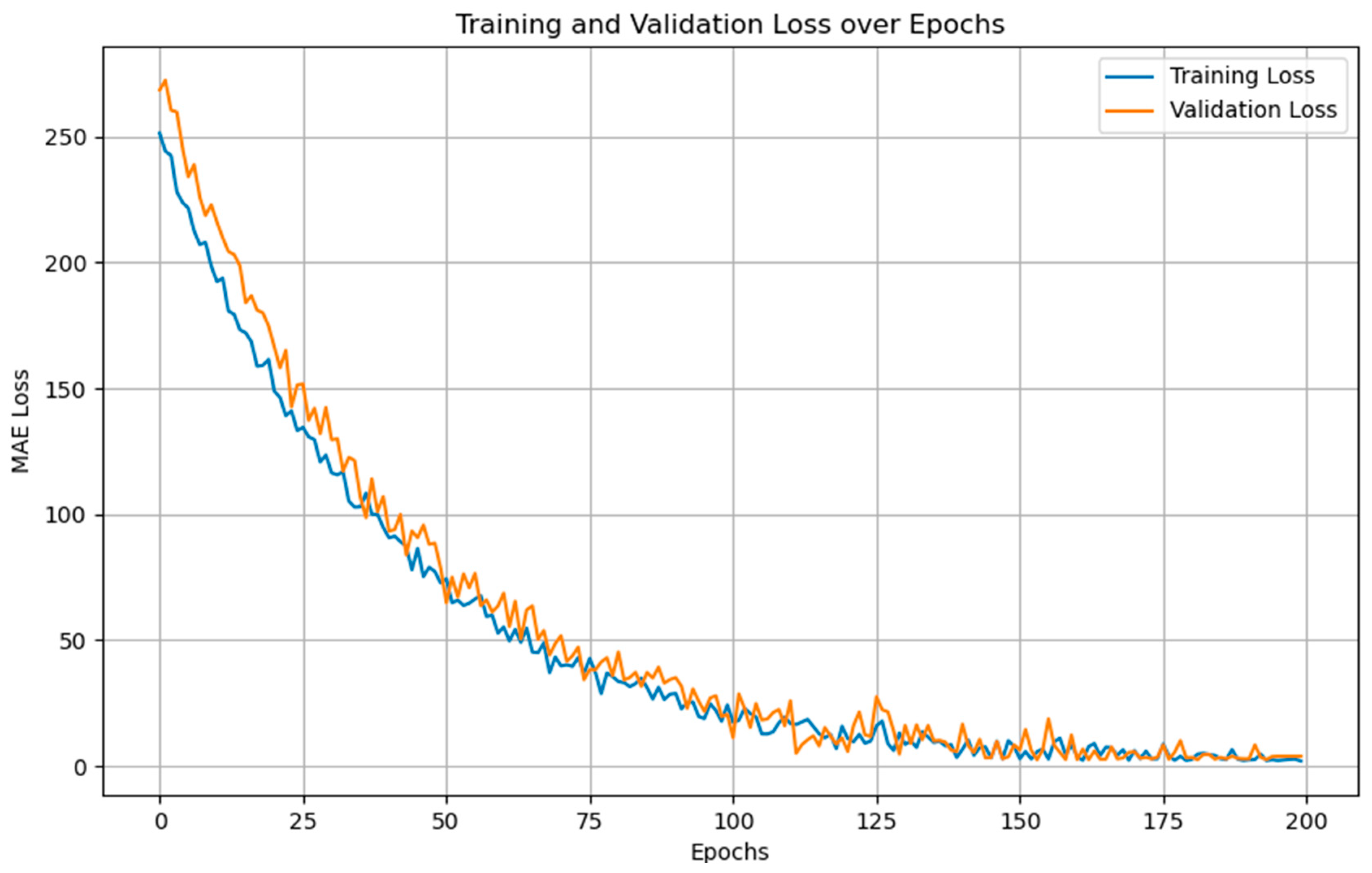
During the training process, we strived to train the loss value of each model to the same level, to ensure the comparability of the performance of each model. Ultimately, through these fine-grained hyperparameter tuning and training strategies, we strove to achieve the best model performance. The loss function of the PGNN model training is shown in Figure 8.

3.4. Analysis

Table 4 compares the average predictive performance of the four models for three metrics using the test set data from monitoring point 2: the purely physics-driven model ECAC, the purely data-driven model DNN, and the two physically fused models HPNN and PGNN. The ECAC model driven by physical methods performed the worst among these models. Its performance was far inferior to the other data-driven models, indicating that a data-driven model has higher accuracy for single-noise event prediction. The DNN model was more accurate than the purely physical approach ECAC. However, its performance was inferior to the hybrid physical machine learning model HPNN, suggesting that physics-driven model output features are effective additional inputs that can significantly improve model performance. The PGNN model performed the best, improving by 22.2%, 24.0%, and 19.1% in MAE, MAPE, and RMSE compared to the DNN. These experiments showed that the fusion model outperformed the physics-driven and machine learning models for single-noise event prediction.
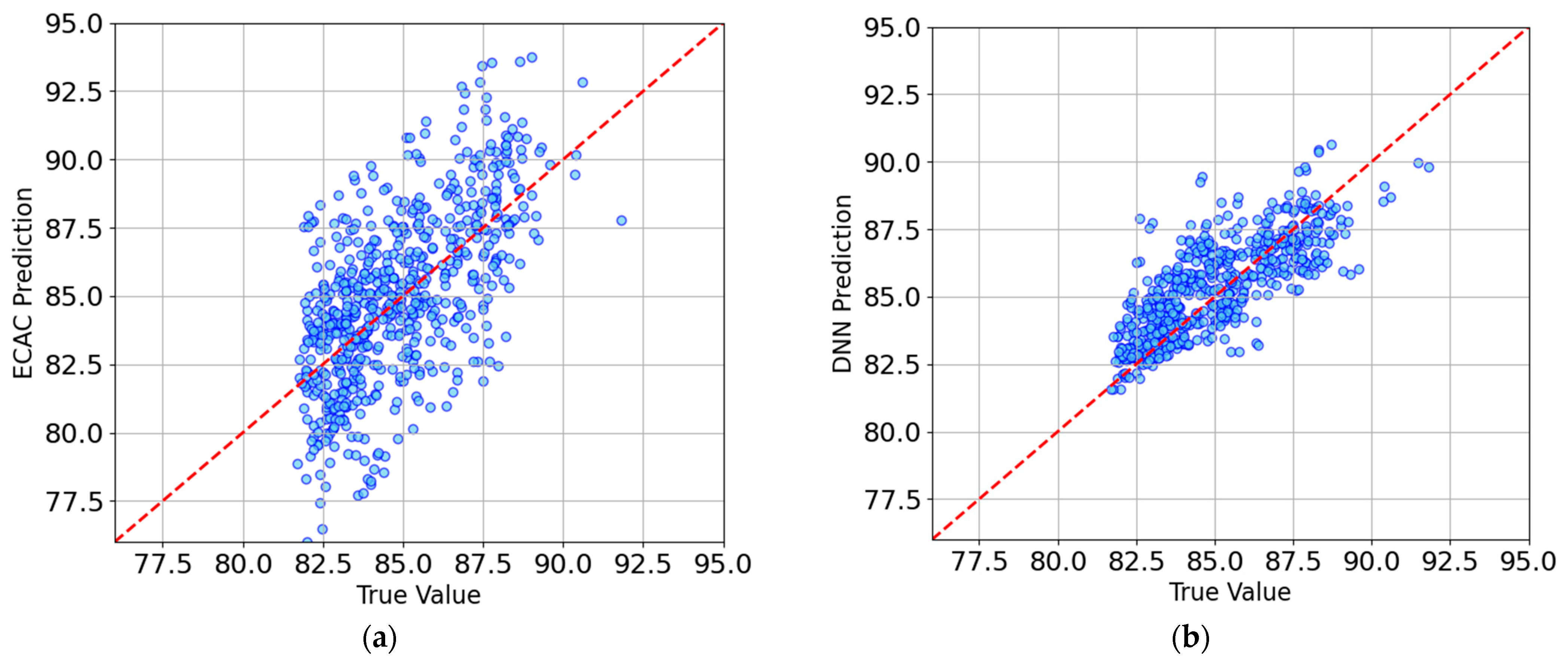
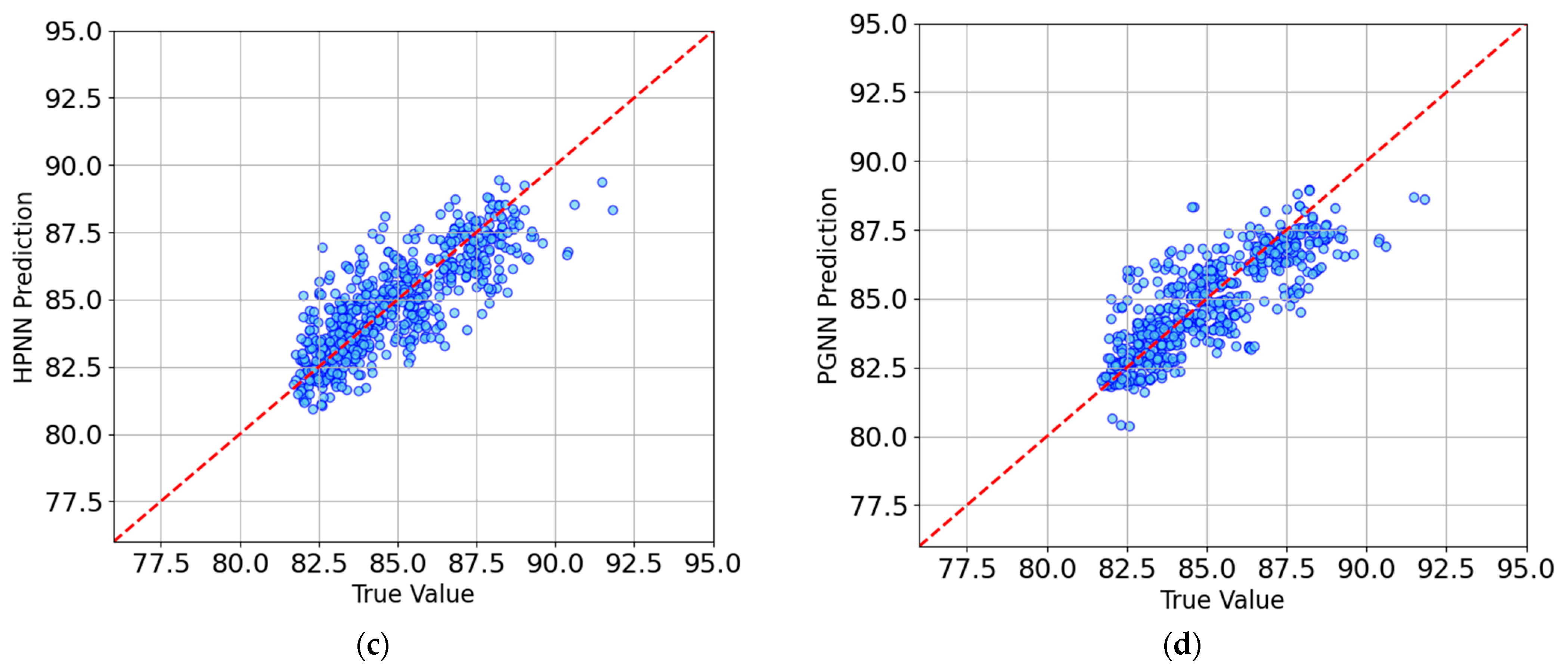
Figure 9 displays scatter plots of the predicted noise values versus actual noise values for the test set of the four models, providing further confirmation of their performance. The scatter distribution in the ECAC model deviated the most from the straight line y = x. The DNN model predicted better than the purely physics-driven model, but its scatter distribution was still dispersed, with a maximum prediction error close to 6 dBA. In contrast, the scatter distribution of the HPNN and PGNN models was more uniform and concentrated on both sides of the line, with an absolute prediction error of less than 5 dBA. Among these models, the PGNN model had the most concentrated scatter distribution and the smallest average absolute error in prediction compared to the HPNN model, indicating that the PGNN model could predict single-event noise values more accurately.
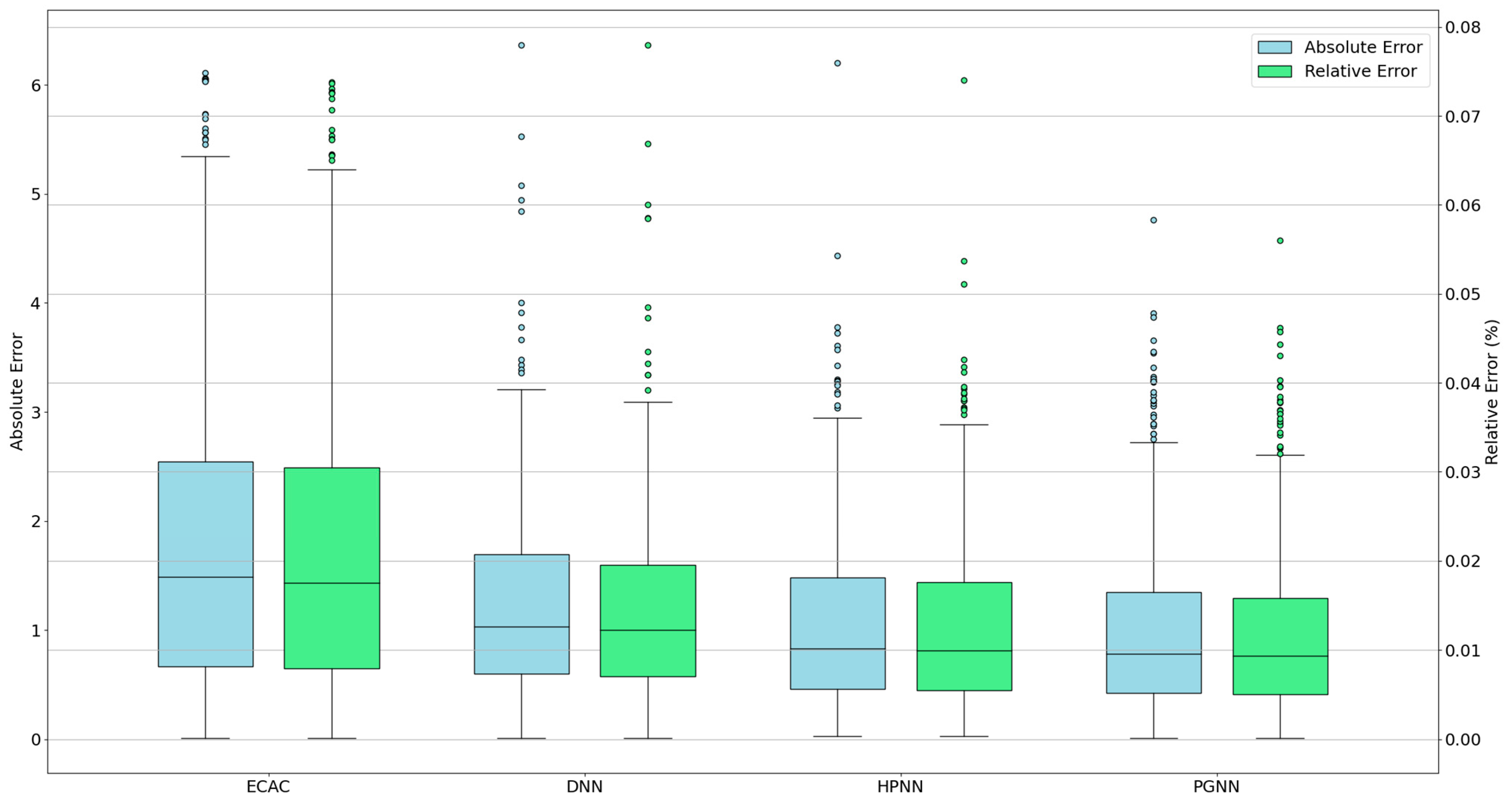
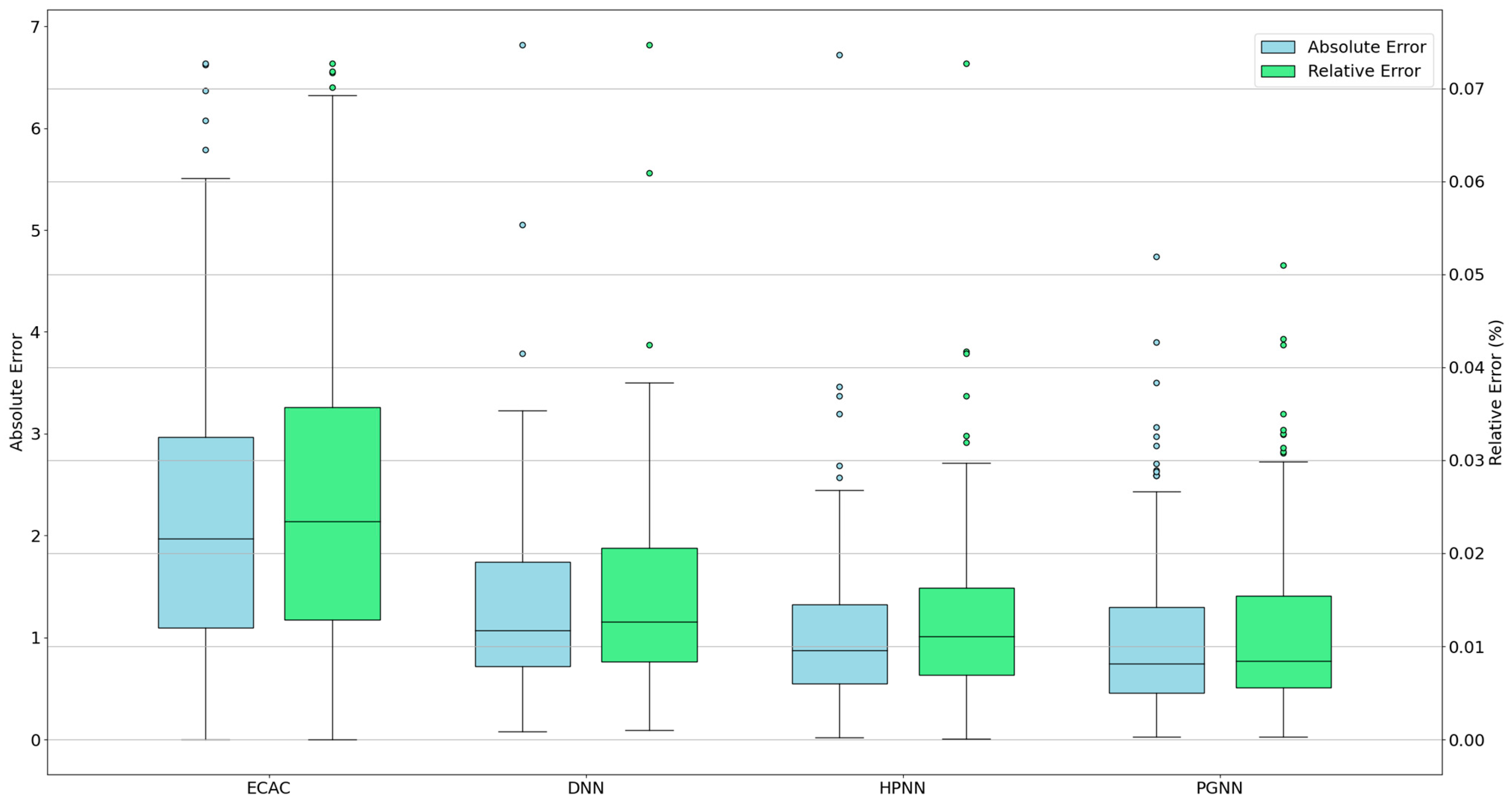
Figure 10 and Figure 11 present the distribution of the absolute and relative errors computed by the four models on the test set for the approach and departure flight attributes through box plots, respectively. It can be seen that the physics-driven ECAC model had the highest absolute and relative prediction errors for the actual data, indicating that this model had a poor ability to capture nonlinear trends. Meanwhile, the traditional physics-driven model exhibited significantly different prediction accuracies for the approach and departure flights, with the prediction accuracy for departure flights significantly lower than that for approach flights. In the machine learning models, the prediction accuracy difference between the approach and departure flights was insignificant, and their prediction results were better than those of the ECAC model. Due to the fusion of physical features, the HPNN and PGNN models performed better than the purely data-driven model, exhibiting good consistency and strong uncertainty adaptability for the noise prediction of single events.
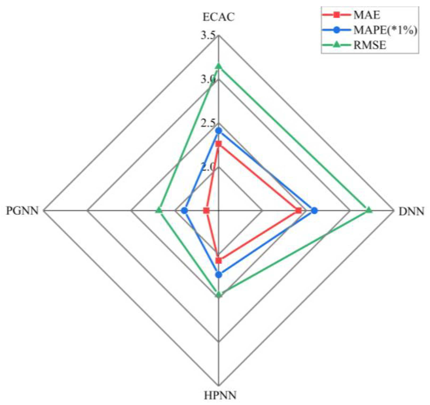
Next, a comprehensive generalization performance evaluation of the four models was performed using the datasets collected at monitoring points 1, 3, and 4. The results are shown in Figure 12. All models except the ECAC model showed a decline in performance on all metrics. The purely data-driven DNN model showed a weaker performance than the ECAC model on the other monitoring datasets, indicating that purely machine learning models depend highly on data quality and perform poorly in extrapolating data. Both the HPNN and PGNN models used physical knowledge as input. Although the overall indicators declined, their prediction performance was still better than the physics-driven ECAC model. This result shows that the data-driven model combined with physical knowledge could effectively learn the overall output trend of the system and show good adaptability to the uncertainty in real data. Among all the constructed models, the PGNN model performed particularly well. This was because the PGNN model not only incorporates physical knowledge into the input layer, but also integrates it into the loss function. This comprehensive approach showed excellent performance in the model generalization test phase. This deep integration of physical knowledge gives PGNN an advantage in dealing with complex practical problems, further proving the importance and effectiveness of physical knowledge in data-driven modeling.
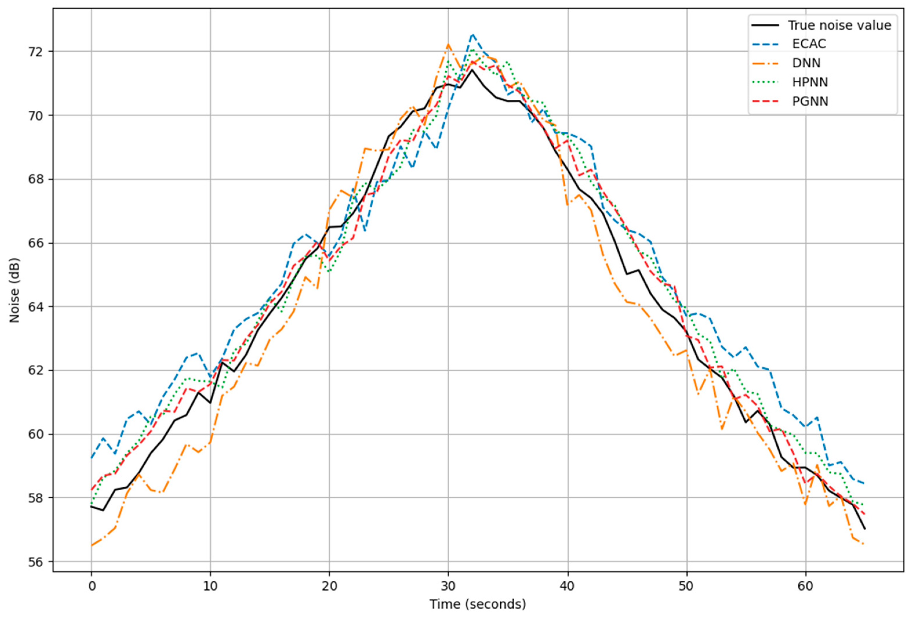
In order to more intuitively demonstrate the evaluation effect of different evaluation models on aircraft noise, we randomly selected an approach flight from the test set and plotted a line graph of the measured noise value and the evaluation value of each model, as shown in Figure 13. From the figure, we can clearly see that the error of the ECAC model in the actual prediction was relatively large. This may have been due to the fact that the physical model found it difficult to fully capture all factors affecting noise in a complex and changeable real environment. In contrast, although the deep neural network (DNN) model can automatically learn complex patterns in the data, its prediction results also had certain deviations, indicating that a single data-driven method also has limitations when facing complex problems.
The HPNN and PGNN models showed better performance by cleverly incorporating the evaluation value of the ECAC model as guidance information into their prediction process. These two models not only effectively utilized the prior knowledge of the physical model, but also further mined potential information in the data through deep learning technology, thereby achieving a significant improvement in prediction accuracy. In particular, the PGNN model, by explicitly adding physical guidance terms to the loss function, had prediction results that were more accurate than the HPNN, further verifying the important role of physical guidance in improving the prediction ability of the model.

4. Conclusions

This paper addressed the problem of single-event noise at airports by proposing a new model based on physics-guided neural networks. This model combines the classical ECAC model with machine learning techniques to improve the accuracy of aircraft noise prediction. Specifically, we introduced the PGNN framework, which incorporates physical knowledge into the loss function to ensure that the model’s outputs are consistent with the laws of physics. To compare our PGNN model with other existing models, we constructed four models: an ECAC physics-driven model, a DNN data-driven model, an HPNN hybrid physical model, and a PGNN physics-guided model. The experimental results showed that the physical model was less adaptable to data dispersion and uncertainty, especially when dealing with nonlinear systems with multiple external perturbations, such as aviation noise. The results demonstrated that the physics-guided neural network inherited the advantages of both physical models and machine learning approaches. It provided accurate and reliable predictions while being more adaptable to changes in the data. Our approach offers a promising solution to the airport single-event noise problem and can contribute to developing effective noise mitigation strategies.

Author Contributions

Conceptualization, D.Z. and C.D.; Methodology, D.Z. and J.P.; Investigation, D.Z. and C.D.; Data curation, D.Z. and J.P.; Supervision, D.Z.; Validation, C.D. and J.P.; Writing—original draft preparation, D.Z. and C.D.; Writing—review and editing, D.Z. and J.P. All authors have read and agreed to the published version of the manuscript.

Funding

This work was funded by the National Key R&D Program of China (No. 2022YFB2602403) and the State Key Laboratory of Air Traffic Management System and Technology (No. SKLATM202007).

Data Availability Statement

The data supporting the findings of this study are available from Hefei Xinqiao International Airport. However, the availability of these data is restricted, and the data were used for this study under license and are therefore not publicly available. However, the authors can provide the data upon reasonable request and with the permission of Hefei Xinqiao International Airport.

Acknowledgments

We would like to thank the National Air Traffic Control Flight Flow Management Technology Key Laboratory of Nanjing University of Aeronautics and Astronautics for providing the data used in the model tests described in this paper.

Conflicts of Interest

The authors declare no conflicts of interest.

References

  1. Jackson, D.C.; Rindfleisch, T.C.; Alonso, J.J. A system for measurement and analysis of aircraft noise impacts. Eng. Proc. 2021, 13, 6. [Google Scholar] [CrossRef]
  2. Pretto, M.; Giannattasio, P.; De Gennaro, M.; Zanon, A.; Kühnelt, H. Web data for computing real-world noise from civil aviation. Transp. Res. Part D Transp. Environ. 2019, 69, 224–249. [Google Scholar] [CrossRef]
  3. Pretto, M.; Giannattasio, P.; De Gennaro, M.; Zanon, A.; Kuehnelt, H. Forecasts of future scenarios for airport noise based on collection and processing of web data. Eur. Transp. Res. Rev. 2020, 12, 4. [Google Scholar] [CrossRef]
  4. Feng, H.; Zhou, Y.; Zeng, W.; Ding, C. Review on metrics and prediction methods of civil aviation noise. Int. J. Aeronaut. Space Sci. 2023, 24, 1199–1213. [Google Scholar] [CrossRef]
  5. Gao, Z.; Mavris, D.N. Statistics and machine learning in aviation environmental impact analysis: A survey of recent progress. Aerospace 2022, 9, 750. [Google Scholar] [CrossRef]
  6. Pretto, M.; Giannattasio, P.; De Gennaro, M. Mixed analysis-synthesis approach for estimating airport noise from civil air traffic. Transp. Res. Part D Transp. Environ. 2022, 106, 103248. [Google Scholar] [CrossRef]
  7. Bertsch, L.; Sanders, L.; Thomas, R.H.; LeGriffon, I.; June, J.C.; Clark, I.A.; Lorteau, M. Comparative assessment of aircraft system noise simulation tools. J. Aircr. 2021, 58, 867–884. [Google Scholar] [CrossRef]
  8. Revoredo, T.; Mora-Camino, F.; Slama, J. A two-step approach for the prediction of dynamic aircraft noise impact. Aerosp. Sci. Technol. 2016, 59, 122–131. [Google Scholar] [CrossRef]
  9. Lukić, M.; Gavran, D.; Fric, S.; Ilić, V.; Vranjevac, S.; Trpčevski, F. Prediction of aircraft noise using machine learning. In Proceedings of the 27th International Congress on Sound and Vibration, Online, 11–16 July 2021. [Google Scholar]
  10. Barron, A.R. Universal approximation bounds for superpositions of a sigmoidal function. IEEE Trans. Inf. Theory 1993, 39, 930–945. [Google Scholar] [CrossRef]
  11. Feng, H.; Zhou, Y.; Ding, C.; Zeng, W.; Guo, W. Aircraft Noise Prediction Based on Machine Learning Model. Trans. Nanjing Univ. Aeronaut. Astronaut. 2023, 40, 54–61. [Google Scholar]
  12. Vabalas, A.; Gowen, E.; Poliakoff, E.; Casson, A.J. Machine learning algorithm validation with a limited sample size. PLoS ONE 2019, 14, e0224365. [Google Scholar] [CrossRef] [PubMed]
  13. Jia, X.; Willard, J.; Karpatne, A.; Read, J.S.; Zwart, J.A.; Steinbach, M.; Kumar, V. Physics-guided machine learning for scientific discovery: An application in simulating lake temperature profiles. ACM/IMS Trans. Data Sci. 2021, 2, 1–26. [Google Scholar] [CrossRef]
  14. Zhou, H.; Qiu, Y.; Feng, Y.; Liu, J. Power prediction of wind turbine in the wake using hybrid physical process and machine learning models. Renew. Energy 2022, 198, 568–586. [Google Scholar] [CrossRef]
  15. June, J.C.; Thomas, R.H.; Guo, Y. System Noise Prediction Uncertainty Quantification for a Hybrid Wing–Body Transport Concept. AIAA J. 2020, 58, 1157–1170. [Google Scholar] [CrossRef]
  16. Gabrielian, A.B.; Puranik, T.G.; Bendarkar, M.V.; Kirby, M.; Mavris, D.; Monteiro, D. Noise model validation using real world operations data. In Proceedings of the 2021 AIAA Aviation and Aeronautics Forum and Exposition, Online, 2–6 August 2021; p. 2136. [Google Scholar]
  17. Simons, D.G.; Besnea, I.; Mohammadloo, T.H.; Melkert, J.A.; Snellen, M. Comparative assessment of measured and modelled aircraft noise around Amsterdam Airport Schiphol. Transp. Res. Part D Transp. Environ. 2022, 105, 103216. [Google Scholar] [CrossRef]
  18. Thomas, R.H.; Burley, C.L.; Guo, Y. Progress of aircraft system noise assessment with uncertainty quantification for the environmentally responsible aviation project. In Proceedings of the 22nd AIAA/CEAS Aeroacoustics Conference, Lyon, France, 30 May 2016; p. 3040. [Google Scholar]
  19. von Rueden, L.; Mayer, S.; Sifa, R.; Bauckhage, C.; Garcke, J. Combining machine learning and simulation to a hybrid modelling approach: Current and future directions. In Proceedings of the Advances in Intelligent Data Analysis XVIII: 18th International Symposium on Intelligent Data Analysis, IDA 2020, Konstanz, Germany, 27–29 April 2020; Proceedings 18. pp. 548–560. [Google Scholar]
  20. Jurj, S.L.; Grundt, D.; Werner, T.; Borchers, P.; Rothemann, K.; Möhlmann, E. Increasing the safety of adaptive cruise control using physics-guided reinforcement learning. Energies 2021, 14, 7572. [Google Scholar] [CrossRef]
  21. Monaco, S.; Apiletti, D.; Malnati, G. Theory-guided deep learning algorithms: An experimental evaluation. Electronics 2022, 11, 2850. [Google Scholar] [CrossRef]
  22. Murphy, C.P.; Kerekes, J.P. Physics-guided neural network for predicting chemical signatures. Appl. Opt. 2021, 60, 3176–3181. [Google Scholar] [CrossRef]
  23. Changdar, S.; Bhaumik, B.; De, S. Physics-based smart model for prediction of viscosity of nanofluids containing nanoparticles using deep learning. J. Comput. Des. Eng. 2021, 8, 600–614. [Google Scholar] [CrossRef]
  24. Karpatne, A.; Atluri, G.; Faghmous, J.H.; Steinbach, M.; Banerjee, A.; Ganguly, A.; Shekhar, S.; Samatova, N.; Kumar, V. Theory-guided data science: A new paradigm for scientific discovery from data. IEEE Trans. Knowl. Data Eng. 2017, 29, 2318–2331. [Google Scholar] [CrossRef]
  25. Uzun, M.; Demirezen, M.U.; Inalhan, G. Physics guided deep learning for data-driven aircraft fuel consumption modeling. Aerospace 2021, 8, 44. [Google Scholar] [CrossRef]
  26. Bode, M.; Gauding, M.; Lian, Z.; Denker, D.; Davidovic, M.; Kleinheinz, K.; Jitsev, J.; Pitsch, H. Using physics-informed enhanced super-resolution generative adversarial networks for subfilter modeling in turbulent reactive flows. Proc. Combust. Inst. 2021, 38, 2617–2625. [Google Scholar] [CrossRef]
  27. Reichstein, M.; Camps-Valls, G.; Stevens, B.; Jung, M.; Denzler, J.; Carvalhais, N.; Prabhat, F. Deep learning and process understanding for data-driven Earth system science. Nature 2019, 566, 195–204. [Google Scholar] [CrossRef]
  28. Cang, R.; Li, H.; Yao, H.; Jiao, Y.; Ren, Y. Improving direct physical properties prediction of heterogeneous materials from imaging data via convolutional neural network and a morphology-aware generative model. Comput. Mater. Sci. 2018, 150, 212–221. [Google Scholar] [CrossRef]
  29. Sadowski, P.; Fooshee, D.; Subrahmanya, N.; Baldi, P. Synergies between quantum mechanics and machine learning in reaction prediction. J. Chem. Inf. Model. 2016, 56, 2125–2128. [Google Scholar] [CrossRef]
  30. Yazdani, A.; Lu, L.; Raissi, M.; Karniadakis, G.E. Systems biology informed deep learning for inferring parameters and hidden dynamics. PLoS Comput. Biol. 2020, 16, e1007575. [Google Scholar] [CrossRef]
  31. Bernardo, J.E.; Kirby, M.; Mavris, D. Development of a rapid fleet-level noise computation model. J. Aircr. 2015, 52, 721–733. [Google Scholar] [CrossRef]
  32. Kim, S.; Lim, D.; Lee, K. Reduced-order modeling applied to the aviation environmental design tool for rapid noise prediction. J. Aerosp. Eng. 2018, 31, 04018056. [Google Scholar] [CrossRef]
  33. Ecac, E. CEAC DOC. 29: Report on standard method of computing noise contours around civil airports, volume 2: Technical guide. In Proceedings of the European Civil Aviation Conference (ECAC), Neuilly-sur-Seine, France, 3 September 2016. [Google Scholar]
  34. Zaporozhets, O.; Levchenko, L. Accuracy of noise-power-distance definition on results of single aircraft noise event calculation. Aerospace 2021, 8, 121. [Google Scholar] [CrossRef]
  35. International Civil Aviation Organization. Recommended Method for Computing Noise Contours Around Airports, 2nd ed.; International Civil Aviation Organization: Montreal, QC, Canada, 2018. [Google Scholar]
  36. Torija, A.J.; Self, R.H. Aircraft classification for efficient modelling of environmental noise impact of aviation. J. Air Transp. Manag. 2018, 67, 157–168. [Google Scholar] [CrossRef]
  37. Synodinos, A.P.; Self, R.H.; Torija, A.J. Framework for predicting noise–power–distance curves for novel aircraft designs. J. Aircr. 2018, 55, 781–791. [Google Scholar] [CrossRef]
  38. Boeker, E.R.; Dinges, E.; He, B.; Fleming, G.; Roof, C.J.; Gerbi, P.J.; Rapoza, A.S.; Hermann, J. Integrated Noise Model (INM) Version 7.0 Technical Manual; Federal Aviation Administration; Office of Environment and Energy: Fairfax County, VA, USA, 2008.
  39. Lee, C.B.E.; Downs, R.; Gorshkov, S.; Hansen, A.; Koopmann, J.; Thrasher, T. Aviation Environmental Design Tool (AEDT) Version 3e Technical Manual; DOT-VNTSC-FAA-22-04; Federal Aviation Administration; Office of Environment and Energy: Fairfax County, VA, USA, 2022.
  40. Berton, J.J. Aircraft Noise and Performance Data for a Notional Supersonic Business Jet. In Proceedings of the 28th AIAA/CEAS Aeroacoustics 2022 Conference, Southampton, UK, 14–17 June 2022; p. 3078. [Google Scholar]
  41. Thomas, J.L.; Hansman, R.J. Modeling, assessment, and flight demonstration of delayed deceleration approaches for community noise reduction. In Proceedings of the 2020 AIAA Aviation and Aeronautics Forum and Exposition, Online, 15–19 June 2020; p. 2874. [Google Scholar]
  42. Rodríguez-Díaz, A.; Adenso-Díaz, B.; González-Torre, P.L. A review of the impact of noise restrictions at airports. Transp. Res. Part D Transp. Environ. 2017, 50, 144–153. [Google Scholar] [CrossRef]
  43. Berton, J.J. Simultaneous use of ground reflection and lateral attenuation noise models. J. Aircr. 2022, 59, 536–543. [Google Scholar] [CrossRef]
  44. Tenney, A.S.; Glauser, M.N.; Lewalle, J. A deep learning approach to jet noise prediction. In Proceedings of the 2018 AIAA Aerospace Sciences Meeting, Kissimmee, FL, USA, 8–12 January 2018; p. 1736. [Google Scholar]
  45. Zellmann, C.; Schäffer, B.; Wunderli, J.-M.; Isermann, U.; Paschereit, C. Aircraft noise emission model accounting for aircraft flight parameters. J. Aircr. 2018, 55, 682–695. [Google Scholar] [CrossRef]
  46. Vela, A.E.; Oleyaei-Motlagh, Y. Ground level aviation noise prediction: A sequence to sequence modeling approach using LSTM recurrent neural networks. In Proceedings of the 2020 AIAA/IEEE 39th Digital Avionics Systems Conference (DASC), Online, 11–15 October 2020; pp. 1–8. [Google Scholar]
  47. Campos, L.M. On physical aeroacoustics with some implications for low-noise aircraft design and airport operations. Aerospace 2015, 2, 17–90. [Google Scholar] [CrossRef]
  48. Isermann, U.; Bertsch, L. Aircraft noise immission modeling. CEAS Aeronaut. J. 2019, 10, 287–311. [Google Scholar] [CrossRef]
  49. Gagliardi, P.; Teti, L.; Licitra, G. A statistical evaluation on flight operational characteristics affecting aircraft noise during take-off. Appl. Acoust. 2018, 134, 8–15. [Google Scholar] [CrossRef]
  50. Torija, A.J.; Self, R.H.; Flindell, I.H. Airport noise modelling for strategic environmental impact assessment of aviation. Appl. Acoust. 2018, 132, 49–57. [Google Scholar] [CrossRef]
  51. Chen, T.; Chen, H. Universal approximation to nonlinear operators by neural networks with arbitrary activation functions and its application to dynamical systems. IEEE Trans. Neural Netw. 1995, 6, 911–917. [Google Scholar] [CrossRef]
  52. Rumelhart, D.E.; Hinton, G.E.; Williams, R.J. Learning representations by back-propagating errors. Nature 1986, 323, 533–536. [Google Scholar] [CrossRef]
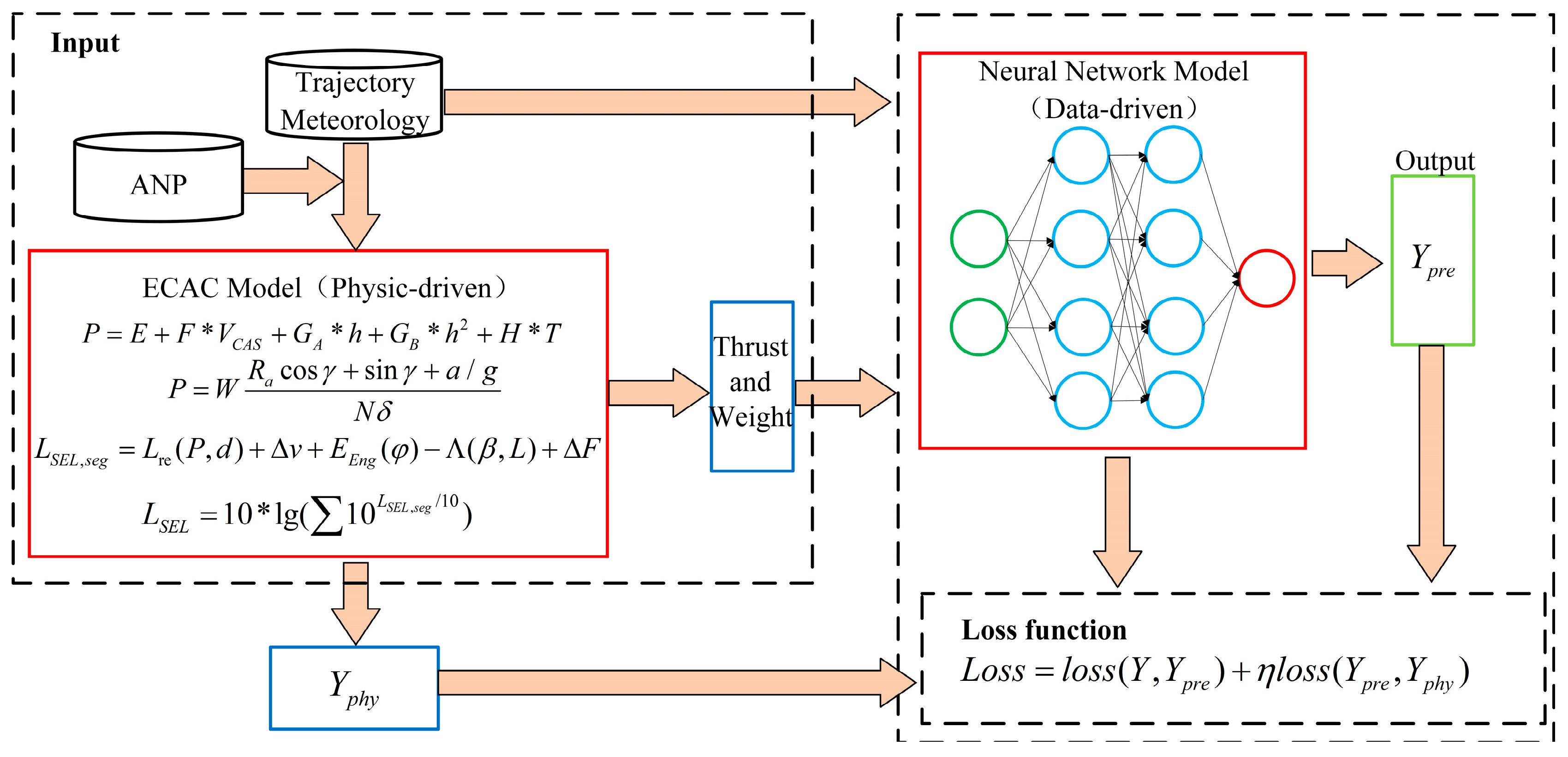
Figure 1. Physics-guided machine learning model.
Aerospace 11 00747 g001
Figure 2. Aircraft–observer angles in the plane normal to the flight path.
Aerospace 11 00747 g002
Figure 3. Position parameters of the aircraft relative to the observer O.
Aerospace 11 00747 g003
Figure 4. Track segments for model input. (a) Track points within 3 NM of the observer’s position; (b) track segments consisting of track points.
Aerospace 11 00747 g004
Figure 5. A single DNN model for aircraft noise prediction.
Aerospace 11 00747 g005
Figure 6. Hybrid physics neural networks for aircraft noise prediction.
Aerospace 11 00747 g006
Figure 7. Layout of noise monitoring points (Station 1 Lat: 32.0112, Lon: 116.9588; Station 2 Lat: 32.0048, Lon: 116.9578; Station 3 Lat: 32.0055, Lon: 116.9626; Station 4: Lat: 31.9594, Lon: 116.9528; yellow represents an approach track, blue represents a departure).
Aerospace 11 00747 g007
Figure 8. Loss value curves for the PGNN model with the final hyperparameter configuration.
Aerospace 11 00747 g008
Figure 9. Scatterplot of predicted and true values of four models (test set). (a) ECAC; (b) DNN; (c) HPNN; (d) PGNN.
Aerospace 11 00747 g009aAerospace 11 00747 g009b
Figure 10. Box plots of relative and absolute errors of arrival flight noise prediction.
Aerospace 11 00747 g010
Figure 11. Box plots of relative and absolute errors of departure flight noise prediction.
Aerospace 11 00747 g011
Figure 12. Performance radar chart for model generalization testing.
Aerospace 11 00747 g012
Figure 13. Prediction chart of arrival flights by different models.
Aerospace 11 00747 g013
Table 1. B772 Departing aircraft weight estimate (from ANP database).
Stage LengthGreat Circle Distance (NM)Weight (lb)
10–500429,900
2500–1000442,400
31000–1500456,100
41500–2500483,100
52500–3500516,400
63500–4500551,700
74500–5500589,400
85500–6500629,500
96500+656,000
Table 2. Main attributes of trajectory data.
Attribute NameAttribute Meaning
Monitoring timeThe point in time at which aircraft trajectory information is collected
LongitudeThe longitude of the aircraft in a spherical space coordinate system
LatitudeThe latitude of the aircraft in the spatial spherical coordinate system
AltitudeThe barometric altitude of the aircraft
Ground speedThe projected ground speed of the aircraft
Flight numberExclusive number of the flight
HeadingThe direction of travel of the aircraft
Table 3. Model parameter configuration.
Model.Hidden LayersNeuronsη
DNN3[64, 64, 32]
HPNN3[128, 64, 32]
PGNN3[128, 64, 32]0.31
Table 4. Sound exposure level prediction accuracy of four models (test set).
ModelMAEMAPERMSE
ECAC2.242.39%3.11
DNN1.261.54%1.57
HPNN1.031.23%1.33
PGNN0.981.17%1.27
Disclaimer/Publisher’s Note: The statements, opinions and data contained in all publications are solely those of the individual author(s) and contributor(s) and not of MDPI and/or the editor(s). MDPI and/or the editor(s) disclaim responsibility for any injury to people or property resulting from any ideas, methods, instructions or products referred to in the content.