1. Introduction
The development of AI for flow approximation is still a young field of science compared to many decades of CFD research. Many approaches have already been pursued and some applications demonstrate the potential of AI methods in forecasting relevant flows in aerospace. Some methodologies abstain from employing AI models for the direct approximation of flow, instead utilizing them to enhance the CFD process [
1]. Conversely, other strategies, such as Physics-Informed Neural Networks (PINNs), directly solve the flow equations [
2,
3], requiring no training database and yielding physically accurate solutions. PINNs can also complement measurement data. In [
4], the flow field was reconstructed using a PINN. Additionally, PINNs have successfully addressed internal flow configurations, solving the steady-state Euler equations in two dimensions for forward and inverse problems [
5]. Furthermore, PINNs have been applied to solve incompressible Navier–Stokes equations. In a separate work [
6], a PINN was utilized to simulate laminar and turbulent flow. The PINN approach was extended to three dimensions in another study [
7]. In this context, the same PINN was enhanced using a data-driven approach, incorporating parameters that describe boundary conditions. The resulting hybrid data-PINNs approach allows for the flexible utilization of various boundary conditions. However, calculating partial differential equations (PDEs) using an AI model is computationally expensive in terms of both time and memory. Consequently, neural networks with relatively few parameters and a simple, typically fully connected structure are chosen. This makes the PINN approach challenging to implement for high-dimensional input spaces, such as design spaces of multi-stage compressors. Additionally, complex AI structures, such as those significantly contributing to the success of Large Language Models (LLMs), cannot be employed.
Other AI models are more oriented towards image recognition and use techniques like convolutional layers [
8]. They require an ordered input, similar to the pixels in an image.
Graph Neural Networks (GNNs), use the computational mesh of the CFD simulations [
9,
10]. They utilize the relationships between adjacent cells to create the flow approximation. This is similar to the successful approach of CFD simulations. GNNs have been successfully used for determining flow quantities in 2D [
11] and 3D [
12]. However, due to the large memory requirements during training, they are limited by the graph size. Various approaches allow GNNs to be applied to larger CFD networks. In reference [
12], the CFD network is divided into sub-meshes. Communication between the sub-meshes occurs through the boundaries with so-called halo cells. Recent methods follow approaches similar to the multigrid approach in CFD solvers [
13], enabling the application of GNNs to CFD meshes with industry-relevant resolution.
The presented method avoids some of the limitations of other AI models by employing the transformer architecture [
14] to approximate the three-dimensional, frictional and compressible flow in compressors.
Compared to PINNs, a high-dimensional input can be used. This allows for a complex CFD setup to be provided as input. Changes in geometry and boundary conditions are directly reflected in the input of the AI model. The degrees of freedom exceed the capabilities of PINNs significantly. As a result, the trained AI model can be used for a wide range of different compressor designs and boundary conditions. Additionally, the AI model employs state-of-the-art architectures with a large number of parameters, which is not possible in the PINN approach.
Moreover, there is no requirement for a CFD grid, as seen in GNNs, to perform the flow approximation. The approximation of the flow at a given point is derived directly from the boundary conditions, which include the geometry and flow boundary conditions for the corresponding operating point. The CFD grid is not incorporated into the AI model, thereby eliminating any memory issues associated with large CFD grids.
Since the structure and resolution of the CFD mesh are not utilized by the AI model, various grid topologies can be employed for training.
Furthermore, the underlying Transformer architecture enables the exchange of information between distant points in the compressor almost directly. Information is not relayed through neighboring points. For example, a separation in the last stage could be communicated immediately to the first stage without requiring any workarounds. This represents a natural advantage of the Transformer architecture.
However, it is not clear whether the abandonment of the neighborhood relationship between the grid cells impairs the approximation quality compared to Graph Neural Networks. In addition, a suitable training database is needed compared to PINNs and the AI approximations can become unphysical.
In summary, this led to the development of a rapid and adaptable AI model capable of generating a comprehensive 3D flow approximation. These flow approximations do not achieve the physical “correctness” of a CFD simulation in terms of the governing differential equations. However, they enable a quick evaluation of an unknown design. These characteristics are comparable to other surrogate models used in the design process of turbomachinery. Surrogate models can showcase their advantages here, as the aerodynamic design of a turbomachinery component, like a compressor stage, is a complex task that requires numerous design variations. Nowadays, automated optimization processes are often used for this design purpose and the generated designs are evaluated and rated using time-consuming CFD simulations. Sophisticated optimization methods reduce the number of required CFD simulations by the intensive use of surrogate models [
15,
16,
17]. These methods significantly speed up the optimization process by making a quite cheap pre-selection of particularly promising candidates in terms of the integral values defining the objectives and constraints. As a result, extensive design analyses with a large number of design variables became possible [
17,
18,
19].
However, these conventional surrogate models, like Gaussian processes [
15,
17], or Radial Basis Function Networks [
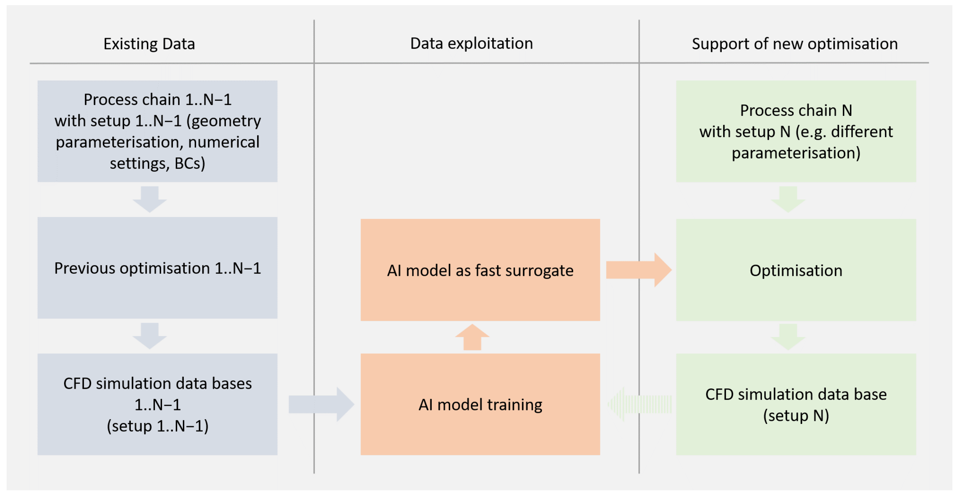
16], only processes and predicts independent scalar-valued results from a specific optimization setup with a fixed set of free variables. This means that the surrogate models have to be built from scratch for each optimization if there is any change in geometry parameterization or in CFD settings, boundary conditions or post-processing to calculate the important evaluation criteria. This paper describes a way to extend the existing surrogate approach which approximates the whole process-chain from design variables to scalar-valued performance criteria, by providing a new AI method that approximates the CFD process and maps the three-dimensional geometry and the respective boundary conditions to the resulting three-dimensional flow. This AI model is able to process the flow of information from millions of cells in a CFD simulation. Compared to many other data-driven surrogate models, this results in a huge knowledge base that can be exploited by the AI model. In addition, the new model can be used flexibly for different compressors and different operating points and it is not tied to a specific design setup. This means that a new design process can be started with an already-trained model. The AI model is able to approximate the 3D flow of newly generated designs in the initial optimization phase.
The possible application of this approach is illustrated in
Figure 1. The left column of
Figure 1 illustrates how CFD results from previous optimizations are collected and then used to train the AI (middle column) for the support of the next upcoming optimization.
The structure of the paper is as follows. First, the developed AI model is described in detail in
Section 2. Then the creation of the training database is explained and the compressor which was analyzed here is presented (
Section 3). The concrete application together with the optimization setup is discussed in
Section 4. The results of the different optimization loops and some aerodynamic details are discussed in
Section 5 and
Section 6. Finally, a brief summary and an outlook are provided in
Section 7.
2. AI Model Structure
The AI model is structured in such a way that input and output are identical to CFD simulations. This means that CFD data can be used directly to train the AI model. Using the CFD data, the AI model learns the relationship between the input boundary conditions (3D geometry coordinates, flow boundary conditions, rotational speed) and the 3D flow (velocities in xyz direction, pressure and density) for any points in the flow.
The AI model is a deep neural network. It uses standardized input and output quantities. This means that all variables have an expected value of zero and a variance of one. Thus, it can be assumed that all input variables have a similar influence on the output of the AI model. This would not be expected for input variables with very different ranges of values. Standardization of the outputs (zero mean, variance one), on the other hand, means that they have a comparable influence on the loss function. Otherwise, outputs with a wide range of values, such as pressure, could dominate the loss function. The loss function is the mean squared error (MSE) of all the output points. Each output point contains the five quantities x, y, and z velocity, density, and pressure. The AI basic structure consists of different modules: a pre-processing module, repeating data processing modules and an interpolation module (
Figure 2).
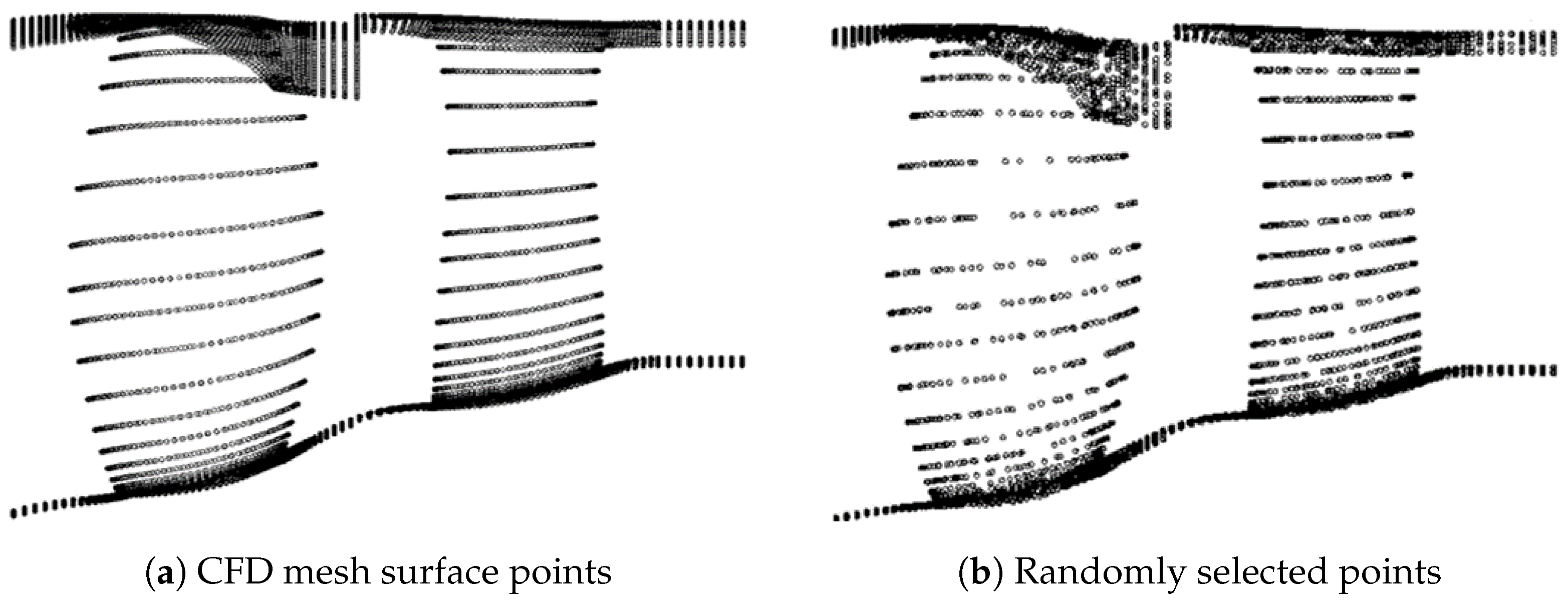
First, the input data are pre-processed. The number of geometry points is reduced to a predetermined number to reduce the memory requirements of the AI model. This is achieved by randomly selecting the surface points of the CFD mesh (
Figure 3).
Typically, blade geometries are described by a limited number of design variables (<100). This means that the blade design can be completely described by a small number of parameters. Consequently, a single design variable changes a large number of geometry points. The influence of a design variable can be fully described by a subset of these geometry points. The number of randomly selected points has been chosen to be sufficiently large for this purpose. The fan stage in
Figure 3 is from a data set described by 64 design parameters. Each parameter change will alter the coordinates of a large number of the 4096 randomly selected points in a row. Depending on the application and the choice of design variables, a different number of randomly selected points may be appropriate. However, a certain degree of universality can be expected. The advantage of using CFD meshes is that they have a very fine resolution in sensitive regions with high flow gradients. On the other hand, uncritical areas can be represented with fewer cells. Therefore, a random selection of points ensures that the distribution of points remains comparable: Areas that are represented by a high resolution in the CFD mesh remain more finely resolved.
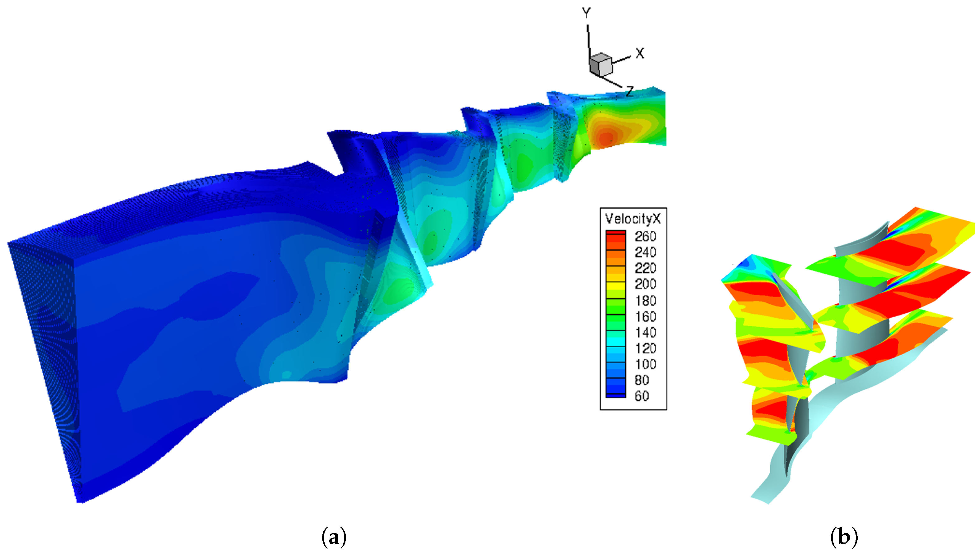
After geometry points are chosen randomly, the turbomachinery compressor is divided into individual blade rows. This enables the use of an AI row model. The AI row model creates an approximation of the 3D flow of one blade passage. As input, it requires the 3D surface coordinates of the blade geometry, the hub and the casing geometry, the rotational speed and the inlet and outlet boundary conditions at the blade row interfaces. This approach allows the AI row model to be used flexibly. The same AI row model can be trained on different compressors with different numbers of stages, blades and vanes because most compressors can be divided into individual blade rows.
Figure 4 shows the AI approximated flow of a 3.5-stage low-pressure compressor (left) and a single-stage fan (right), both of which can be used for training not only the same AI row model, but the entire AI Model.
The goal is to learn from different CFD data and apply them to new applications. Within a single application, this approach results in an enhanced data set for the AI row model: The number of training samples increases with each additional row of blades and vanes in the compressor.
However, to determine the flow in a blade row, the inlet and outlet boundary conditions at the blade row interfaces are required. These are not known everywhere in a multi-row configuration in advance. Therefore, an AI interface model is implemented to approximate the boundary conditions at all interfaces. The AI interface model receives the compressor inlet and outlet conditions as well as the approximations from the AI row model for all compressor stages. This allows flow changes in individual blades and changes in the compressor inlet and outlet to be communicated to all rows. The AI interface model and the AI row model are called iteratively (
Figure 5).
Initially, the AI interface model contains CFD cell coordinates of all interfaces. This location information is used to derive the effects of the compressor inlet and outlet boundary conditions on the interface positions. Each blade row is initially represented by its geometry and rotational velocity. This information is used to initialize the boundary conditions of all interfaces, labeled as “Flow Repr.” in Module 1 of
Figure 5. The AI row model is then called separately for each blade row. It also receives the initial geometry and rotational speed as input. In addition, the AI interface model’s initial estimates of the flow boundary conditions at the blade row interfaces are used. As a result, the AI row model provides an initial flow representation for each blade row. The sequence of AI interface and AI row Model is repeated ten times to increase the degree of freedom and the depth in the AI model. A greater depth of an AI model often enhances the ability to generalize in many cases. However, this has not yet been investigated here.
The sequence commences with an initial setup involving the original geometry and rotational speed. The AI interface models then receive the flow representations from the AI row model, while the row model adopts the boundary conditions from the interface model. Consequently, the boundary conditions at the interfaces and the flow representations undergo iterative updates. In the last step, the flow representation of the AI model is used to approximate the 3D flow. This is conducted using an AI interpolation model.
Due to memory and computational limitations, the AI model cannot use the same number of cells as the CFD mesh for its flow representations. Therefore, the AI model generates an abstract representation of the flow with 4096 points for each row of blades or vanes. Each of these points contains 256 floating-point numbers for storage. In total, the flow in a blade row is represented by 1,048,576 float values. This information is used in the AI interpolation model to interpolate the flow onto the cells of the CFD mesh. Consequently, the AI interpolation model receives the cell-centered coordinates in addition to the flow representations from the AI row model (
Figure 6).
All AI sub-models described above use the Transformer architecture [
14]. In order to increase the stability during training, a modified version has been implemented [
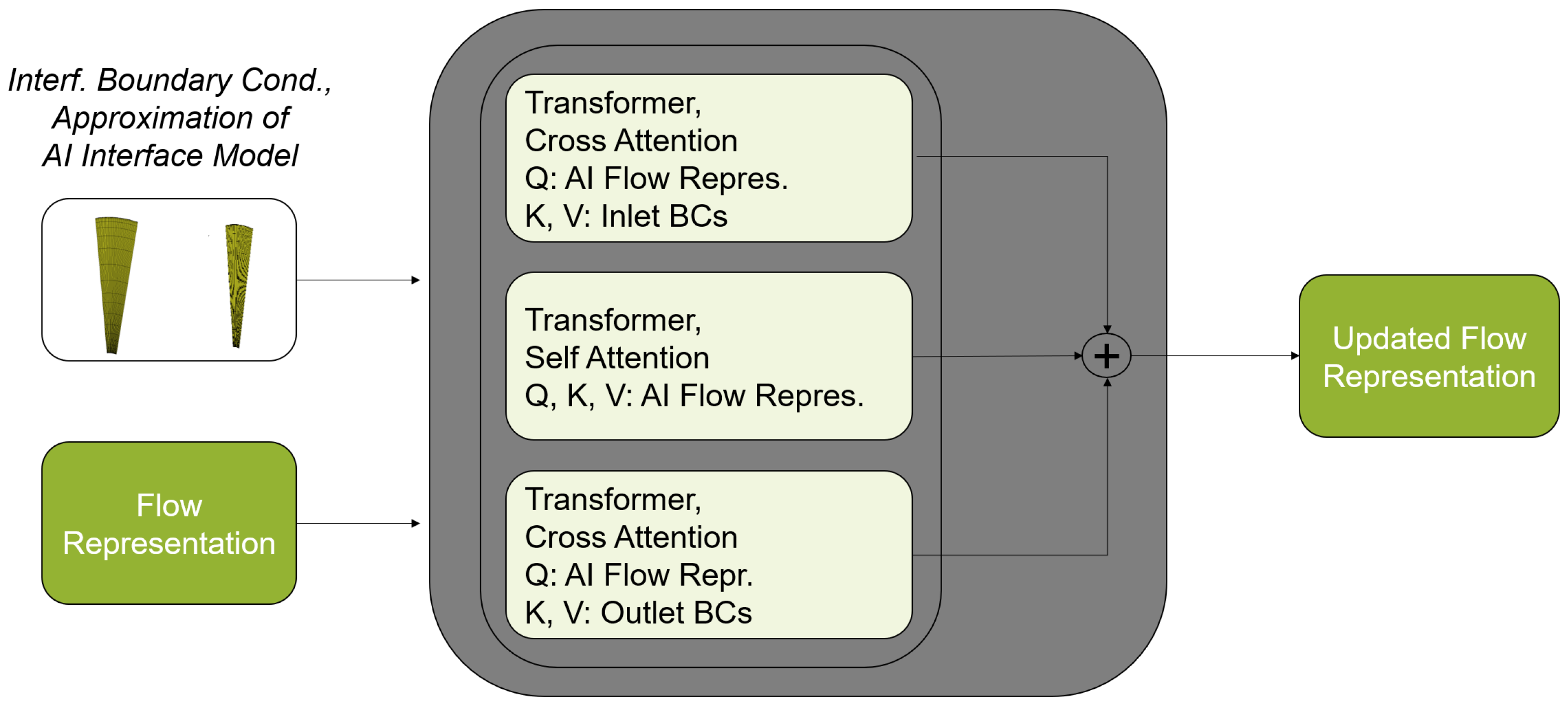
20]. The attention mechanism of the transformer is used in two different ways. Cross-attention is used to add information from other tensors. Self-attention is used to exchange information within a tensor. In the AI interpolation model, only cross-attentions are used to extract the required information from the AI flow representation and to generate the flow approximations for each cell independently. In the cross-attention mechanism, no information is exchanged between the cells, which are the input of the query tensor. For this reason, it is possible to subdivide the cell-centered points of the CFD mesh into any number of subsets. These subsets can be approximated individually. This avoids memory problems even with large CFD meshes.
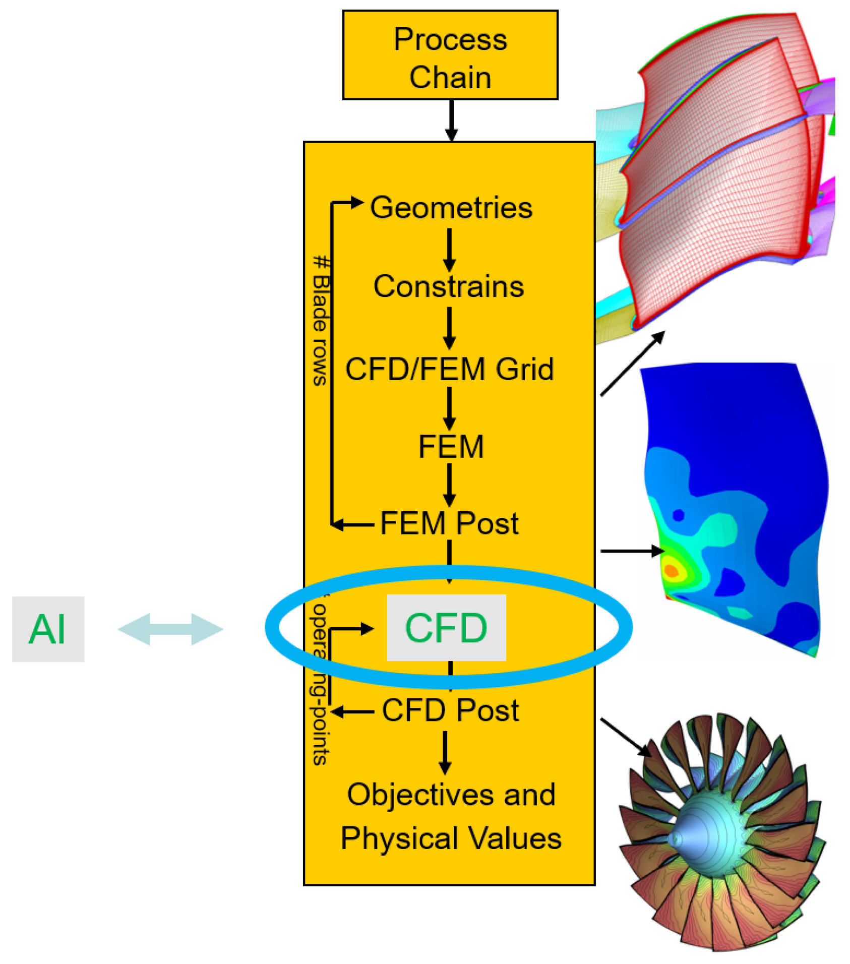
Interpolation onto the CFD meshes and writing of common CFD file formats (e.g., CGNS) allows the same post-processing to be used as in the CFD process chain. The AI model can, therefore, be used as a plug-and-play replacement for CFD simulations in optimization process chains (
Figure 7).
A Transformer call returns an updated query tensor. The key tensor is used to decide which information from the value tensor is relevant [
14]. In
Figure 8 the Transformer calls of the AI row model are displayed. The input elements follow the well-known attention mechanism within the Transformer architecture. They are divided into query, key and value tensors (tensors are multidimensional arrays in this case).
Most layers use 256 units in the last dimension. Exceptions are a layer in the transformer, where the units are increased to 1024, and the input and output layers. The number of units determines the degree of freedom in the AI model. The choice of 256 units results in a total of approx. 47 million trainable parameters.
The AI model is programmed in Python. To implement the AI routines, TensorFlow is used as a library.
3. Training of the AI Model
The training data originates from a design optimization of a three-and-a-half-stage low-pressure compressor. The aim of the optimization was to extend the compressor map at lower speeds and keep the efficiency at the design point. For the compressor map calculation a through-flow method, described in [
19], was used. Additionally, several operating points throughout the map were constantly checked during the optimization using a RANS solver. The RANS calculations were performed with the DLR in-house solver TRACE [
21,
22].
A total of 198 parameters were used to modify compressor geometry and operating points; 110 parameters were used to describe hub and casing contours as well as blade axial chords (
Figure 9). In addition, 73 airfoil parameters were used to define five airfoil sections for each blade. The airfoil parameters are typical for a throughflow solver. Parameters used for the rotor airfoil sections are stagnation pressure ratio, thickness-to-chord ratio and design incidence and for the stator sections thickness-to-chord ratio, outflow angle and design incidence. The remaining parameters include blade numbers, mass flow at ADP, shaft speed and twist angles for the vane schedule at part speed.
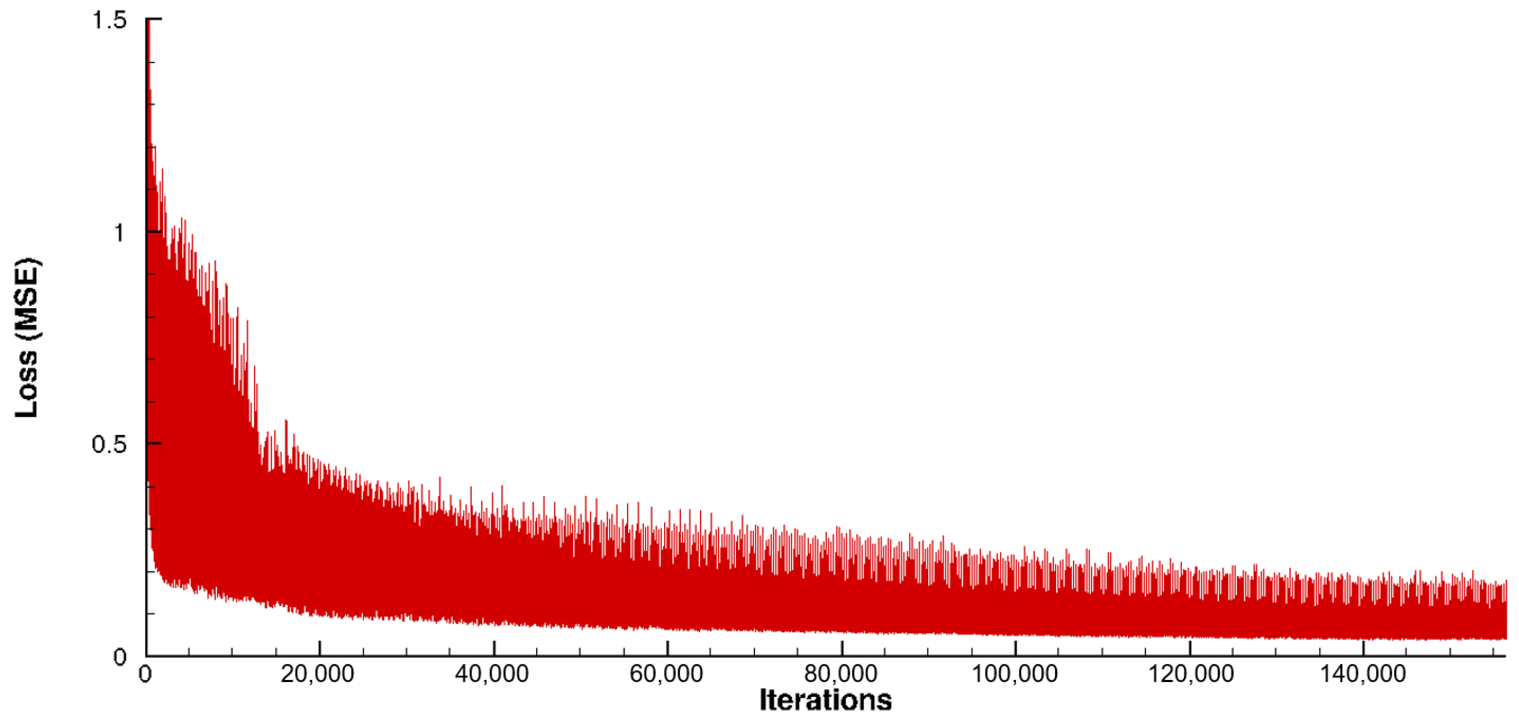
The RANS simulations of this optimization are used as training data for the AI model. The total number of CFD simulations used is 500 and in addition, data augmentation is applied to increase the number of training samples. This is conducted by randomly and independently rotating each blade row in the circumferential direction. The entire compressor is also randomly shifted in the axial direction. These operations do not change the solutions of the CFD simulations, since the data used are stationary, circumferentially periodic RANS simulations. For the AI model, however, new geometries are introduced as input. These extend the training database and should lead to a better generalization of the AI model. This way, the number of training samples is increased to 1500. Training with this database takes 4 days (one GPU, NVIDIA RTX A6000, 48 GB). The development of the loss function, explained in
Section 2, during the training process, is shown in
Figure 10 where the loss over each sample (Mean Squared Error of a single CFD simulation at randomly selected grid points) is plotted, rather than the loss over the epochs as is usually the case.
The plot shows the variation in the MSE of the samples due to the different geometries and operating points. Only one sample is used in each training iteration. This is due to the memory requirements of both the samples and the AI model. In order to be able to use arbitrary mini-batch sizes, a gradient accumulation method was implemented. The gradients from each training iteration are summed up and the result is stored. The actual gradient step to update the parameters of the AI model takes place after a given number of training iterations, in this case, every 16 iterations. As only one sample is used in each iteration, the mini-batch size is also 16.
4. Optimization Setup
As described in the previous sections the AI model can be used to predict flow fields, even if there are changes in geometry parameterization, CFD settings, boundary conditions, or post-processing. Here, it is used to demonstrate how a data set from an early-stage design optimization with typical design parameters of a throughflow method can be used to train an AI model to provide fast predictions for a more detailed CFD design optimization.
The previous throughflow-based setup is adapted for a full 3D RANS CFD optimization. The objectives were reduced to maximizing efficiency at the design point. The different operating points were retained for comparison between CFD simulation and AI approximation but were not included in the objectives.
The 73 airfoil parameters from the through-flow optimization are omitted. Instead, 155 typical design variables such as stagger angles, leading/trailing edge angles, leading/trailing edge radii and De Boor point coordinates for suction and pressure sides are introduced. In total, this optimization setup has 280 free parameters. To limit the number of RANS calculations, only two simulations on each of the four speed lines are carried out, as marked in
Figure 11.
The choice of training data ensures that the AI model is based on data that is close to the use case. The new parameterization requires the AI model to extrapolate to unknown geometry variations.
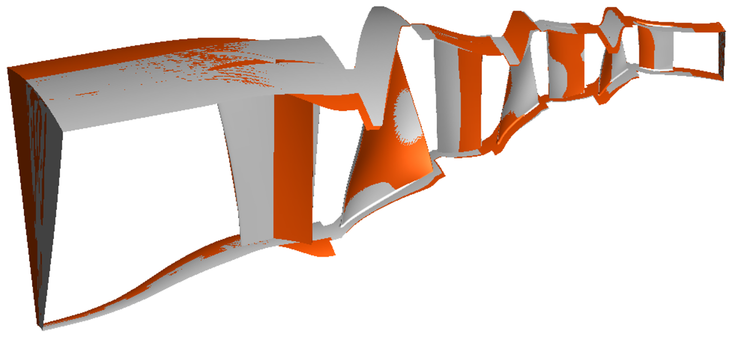
Figure 12 shows the geometric differences between a through-flow parameterized training design and an optimization design using the detailed parameterization described above.
The design space is already limited by the preliminary design. Local design changes are evaluated with the time-consuming and costly CFD process chain. However, these have a significant overall effect on the flow in the compressor. Larger design changes result from the vane schedule. This can be clearly seen on the inlet guide vane (IGV) and stator 1 in
Figure 12. In total, the design variations extend over the entire compressor.
The high number and the variation of design parameters have the following consequences: surrogate models that are only trained during the three-dimensional CFD optimization (e.g., Kriging models) cannot yet deliver reliable results at the beginning of this optimization due to missing data. On the other hand, the pre-trained AI model does not receive the design parameters as direct input but creates the flow solution directly based on the geometries, interfaces and boundary conditions. The AI model does not establish a direct correlation between design parameters and flow solutions. The AI model is, therefore, intended to complement, rather than replace, established optimization surrogate models such as Gaussian processes.
The optimization setup was chosen such that the optimization surrogate models did not play a role in this analysis, as only the initial phase of an optimization was considered. In these studies, the optimizations were terminated after 100 successful runs of the process chain (geometry generation, mesh generation, CFD simulations or AI approximations, post-process). Two independent optimizations were carried out, one was purely CFD-based and the other purely AI-based. The databases were then recalculated and compared using the other model. The CFD optimization should demonstrate that the AI model can deliver meaningful results for the initial phase, a “typical” optimization database. The optimization based on the AI model, on the other hand, could exploit the weaknesses of the model and specifically favor designs with errors in the AI approximation.
Run times for the CFD operating points were between 5 and 15 min (2 CPUs, Advanced Micro Devices, Inc. (AMD), Santa Clara, CA, USA, EPYC 7601, 32 cores, 2.2 GHz). The AI approximation of an operating point took 10 to 15 s (one GPU, NVIDIA, Santa Clara, CA, USA, RTX A6000, 48 GB). With finer CFD meshes, the speed advantage of the AI model would probably increase further. In addition, the AI approximations naturally do not show any convergence problems compared to CFD solvers.
5. Results
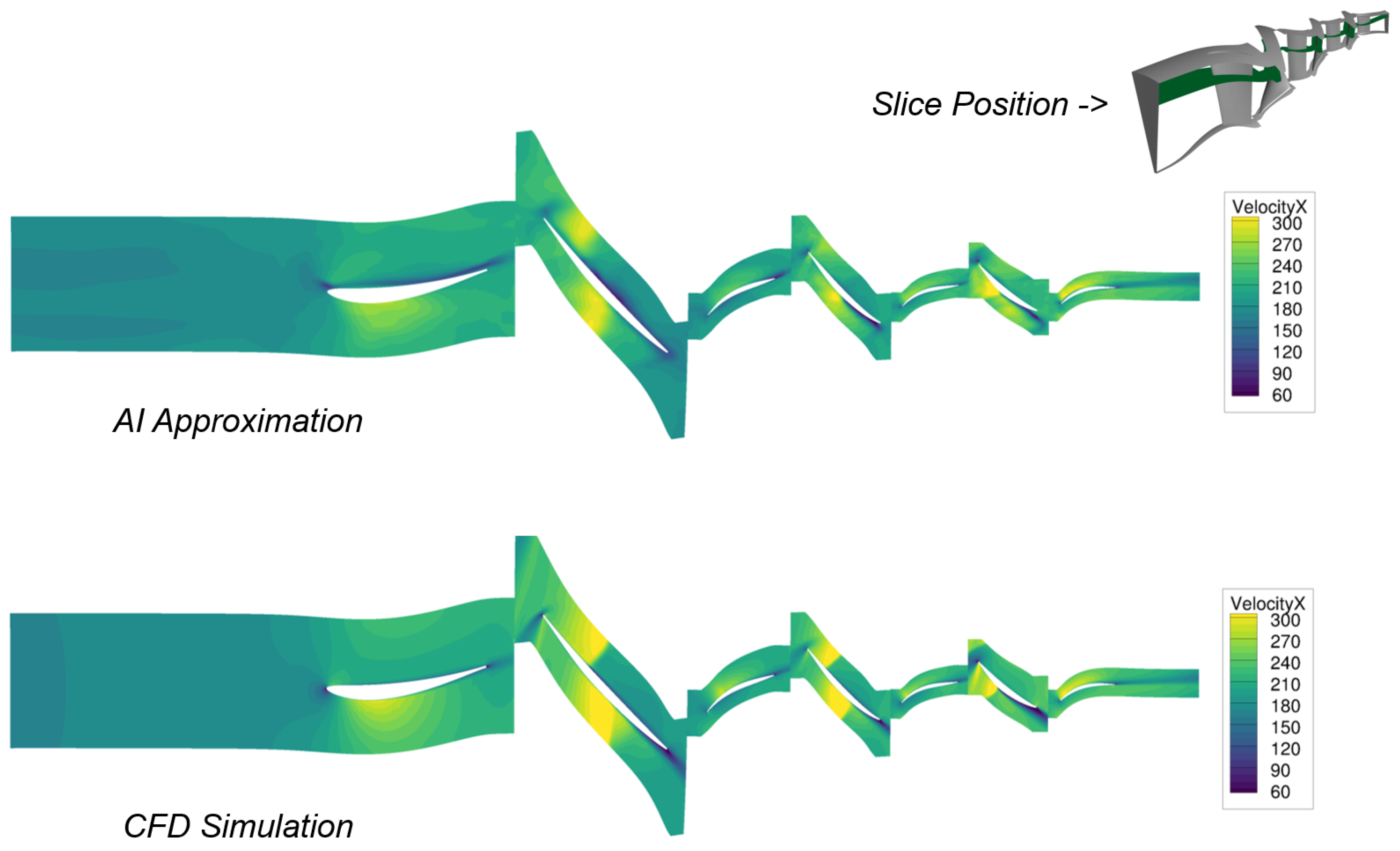
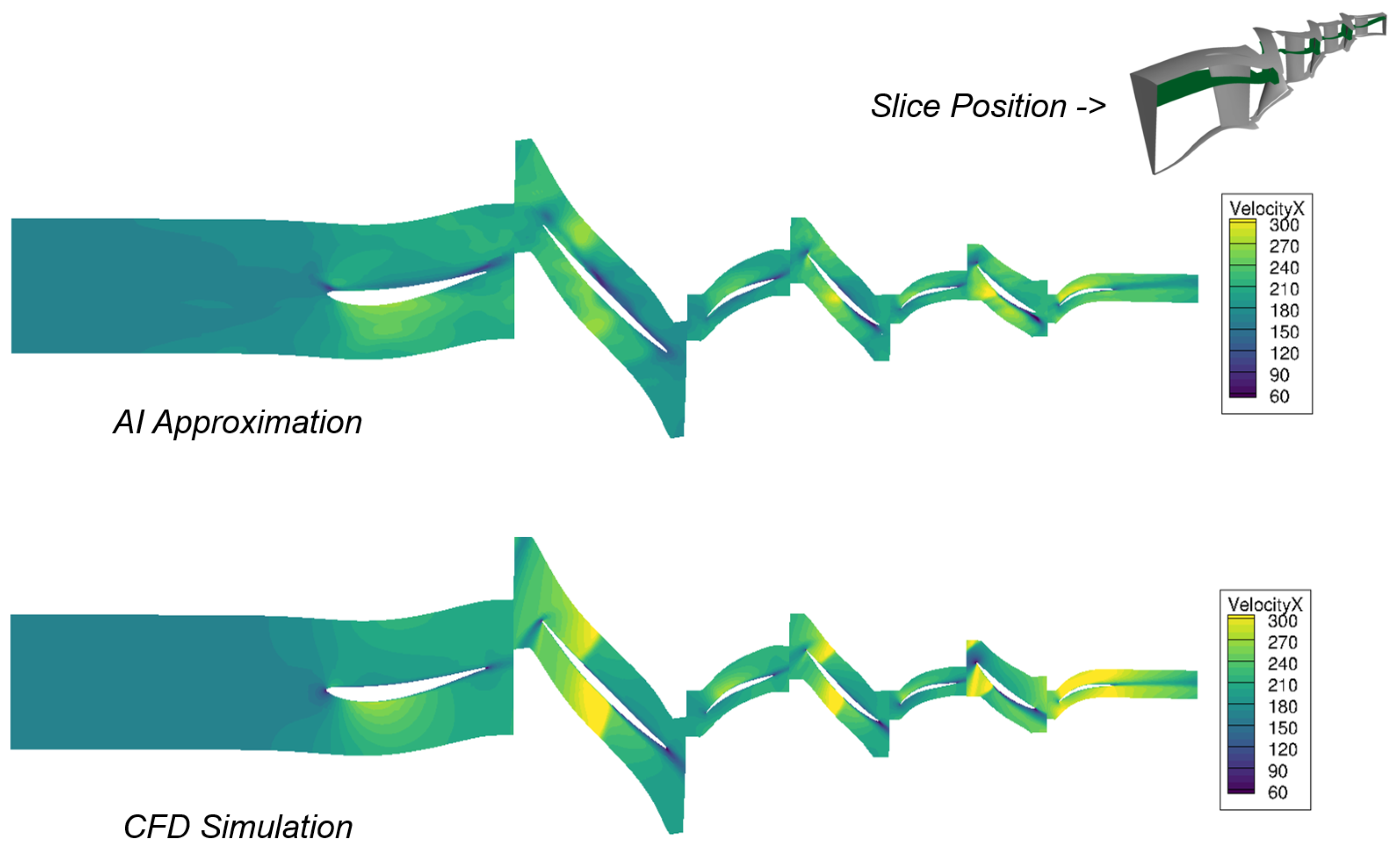
To gain an initial impression of the extent to which the model can approximate the flow physics learned from the RANS simulations,
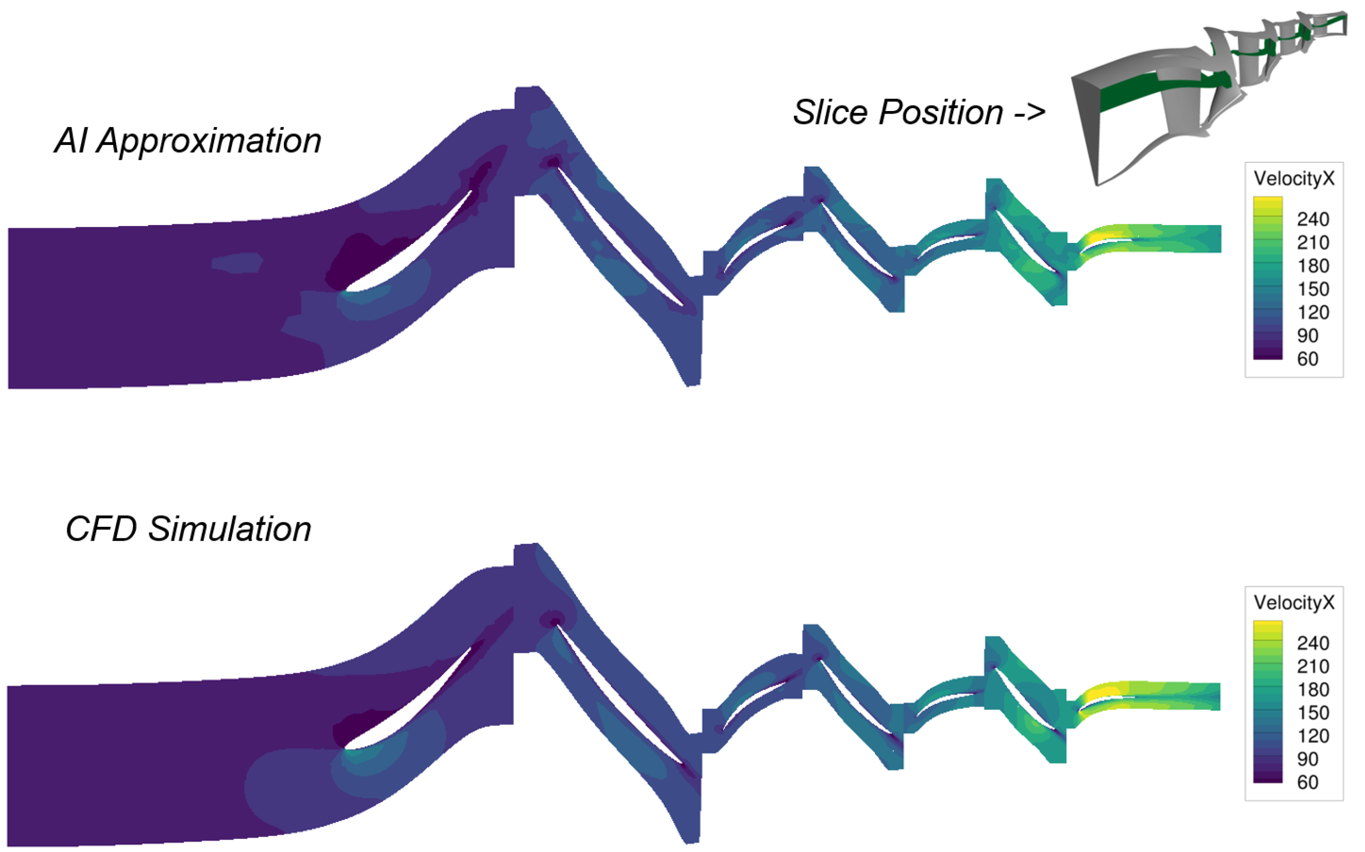
Figure 13 shows a comparison of the flow velocities in the axial direction for the aerodynamic design point at 100% rotational speed.
A design from the initial phase of the CFD optimization process was selected for this comparison and recalculated with the AI model. A meridional section through the three-dimensional flow solution is presented to facilitate a comparison between CFD and AI flow. Therefore, the axial velocity is depicted.
Qualitatively, the AI approximation seems to provide a sufficiently accurate representation of the flow field. The overall velocity level remains consistent. The flow surrounding the blades is illustrated, and the shock system is clearly visible. Significant deviations are observed in rotor 2, where the AI model fails to clearly delineate the shock. Generally, the AI model tends to blur the sudden change in the velocity at the shock position, generating a large local error (
Figure 14).
Figure 15 presents a different operating point on the working line at 70% part speed.
The alteration in the velocity field, induced by the reduced shaft rotation, is portrayed by the AI model. In general, the flow across all operating points is depicted with comparable quality. Stagnation points and wakes are distinctly visible.
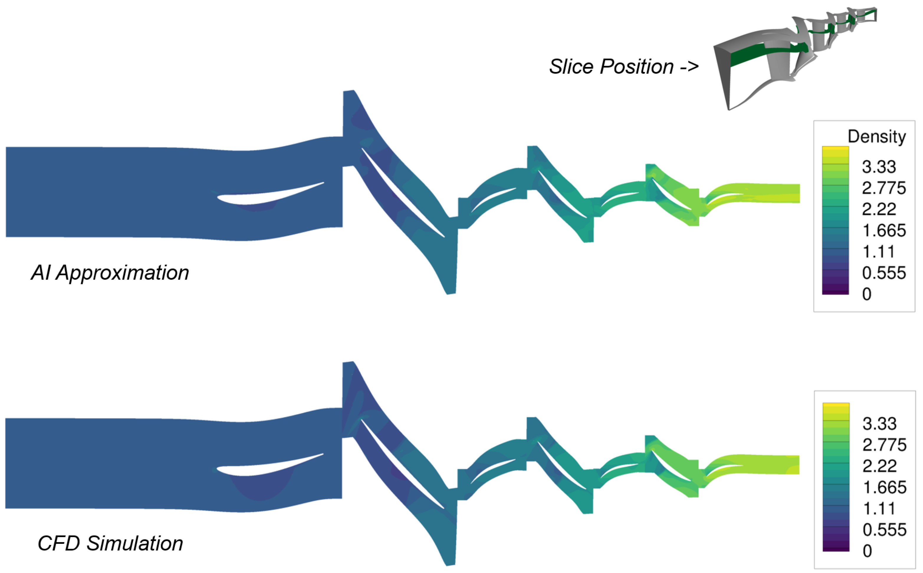
The AI model approximates the velocities, density, and pressure. All quantities are represented with similar quality. This is exemplified by the approximation of the density in
Figure 16.
The AI model was trained to minimize the mean squared error (MSE) between the AI approximation and CFD simulations of the complete flow field. This enables the AI model to reproduce many of the characteristics in the flow pattern. However, what is particularly important for an optimization setup is how the discrepancies between CFD and AI flow solutions influence the integral quantities of the optimization. For example, small differences in the flow can have a major influence on the efficiency, which is used as an objective function in almost all aerodynamic compressor optimizations and should be maximized. Such integral quantities were not explicitly taken into account in the training of the AI model but would be automatically reproduced if the AI approximations were of sufficient accuracy. Deviations in the AI approximations as shown in
Figure 13 and
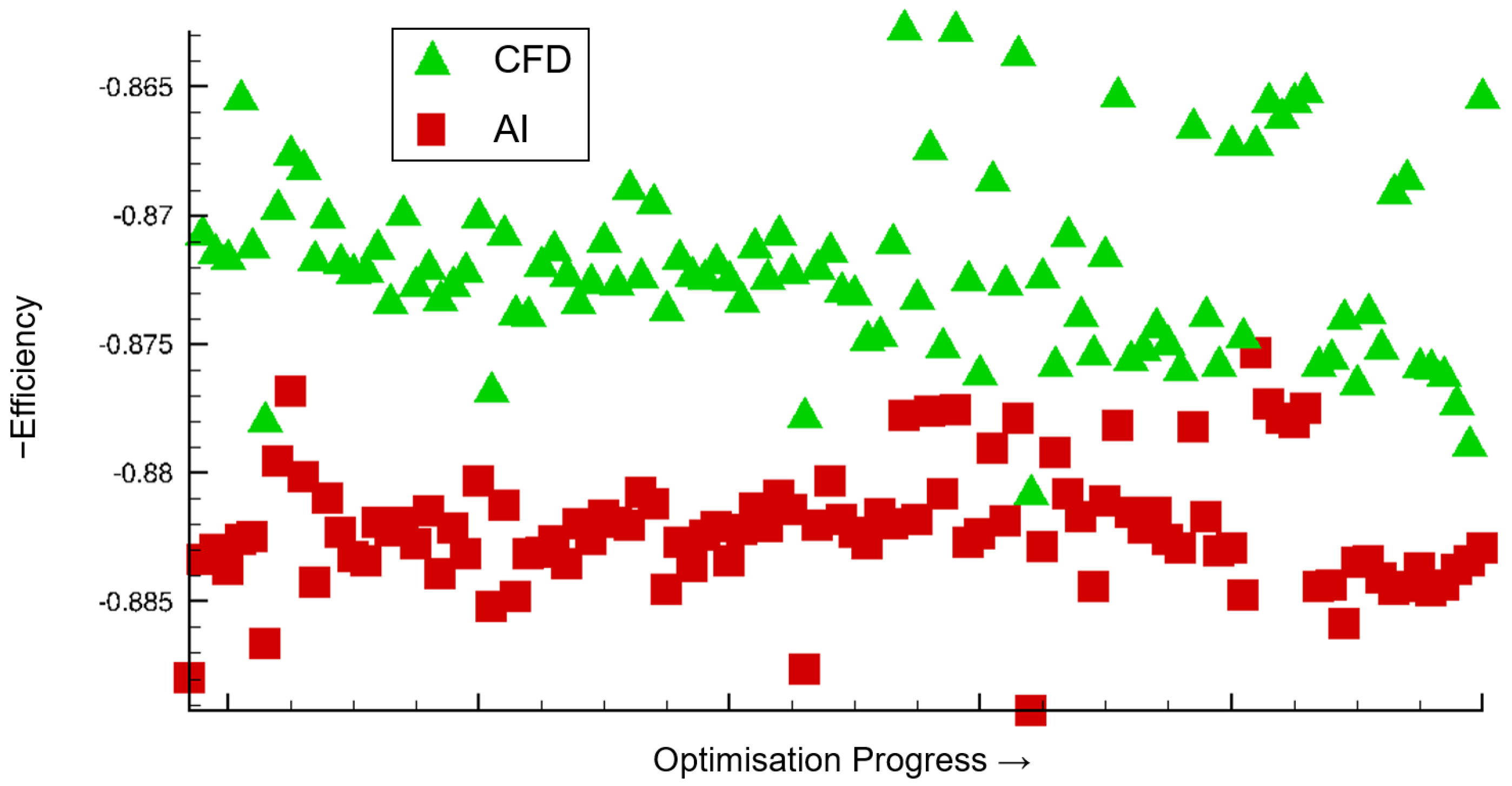
Figure 15 suggest, however, that a sensitive variable such as efficiency could not be reproduced accurately. This assumption is confirmed in
Figure 17. It is important to note that the isentropic efficiency of a compressor (see [
23] for the definition of compressor performance parameters) is calculated solely from inlet and outlet flow quantities (total pressure and total temperature), while the loss function of the AI model is based on the reproduction of entire flow field. This means that even very small changes in the total temperature at the compressor outlet have a very strong effect on the efficiency, but hardly any effect on the loss function of the AI model. Consequently, this performance parameter represents a significant challenge for the AI model. Nevertheless, it is typically incorporated into the majority of compressor optimization processes.
Within an optimization process, surrogate models are typically used to quickly evaluate new designs. Therefore, the representation of the optimization progress was chosen here. This is intended to illustrate whether the AI model could be used to filter out a newly generated design.
The isentropic efficiencies of the optimization designs, calculated by conventional post-processing of the respective CFD or AI flow solution, are represented over the optimization progress. This axis is determined by the order in which the designs were calculated. The further to the right a design is on the progress axis, the later it was generated. Later designs benefit from already calculated designs. Thus, promising designs can inherit their parameters.
Designs that did not successfully pass through the process chain have been sorted out in this representation. CFD and AI results with the same value on the optimization progress axis refer to the same design.
It is immediately apparent that the efficiencies calculated from the AI approximation are generally approx. 1% too high (the negative values of the efficiency are plotted because fitness functions are minimized in the optimization). An error of one percent in efficiency is generally significant when optimizing a compressor. Because often the efficiency can only be increased slightly. A positive evaluation by the AI model could, therefore, be solely due to the inaccuracy of the model.
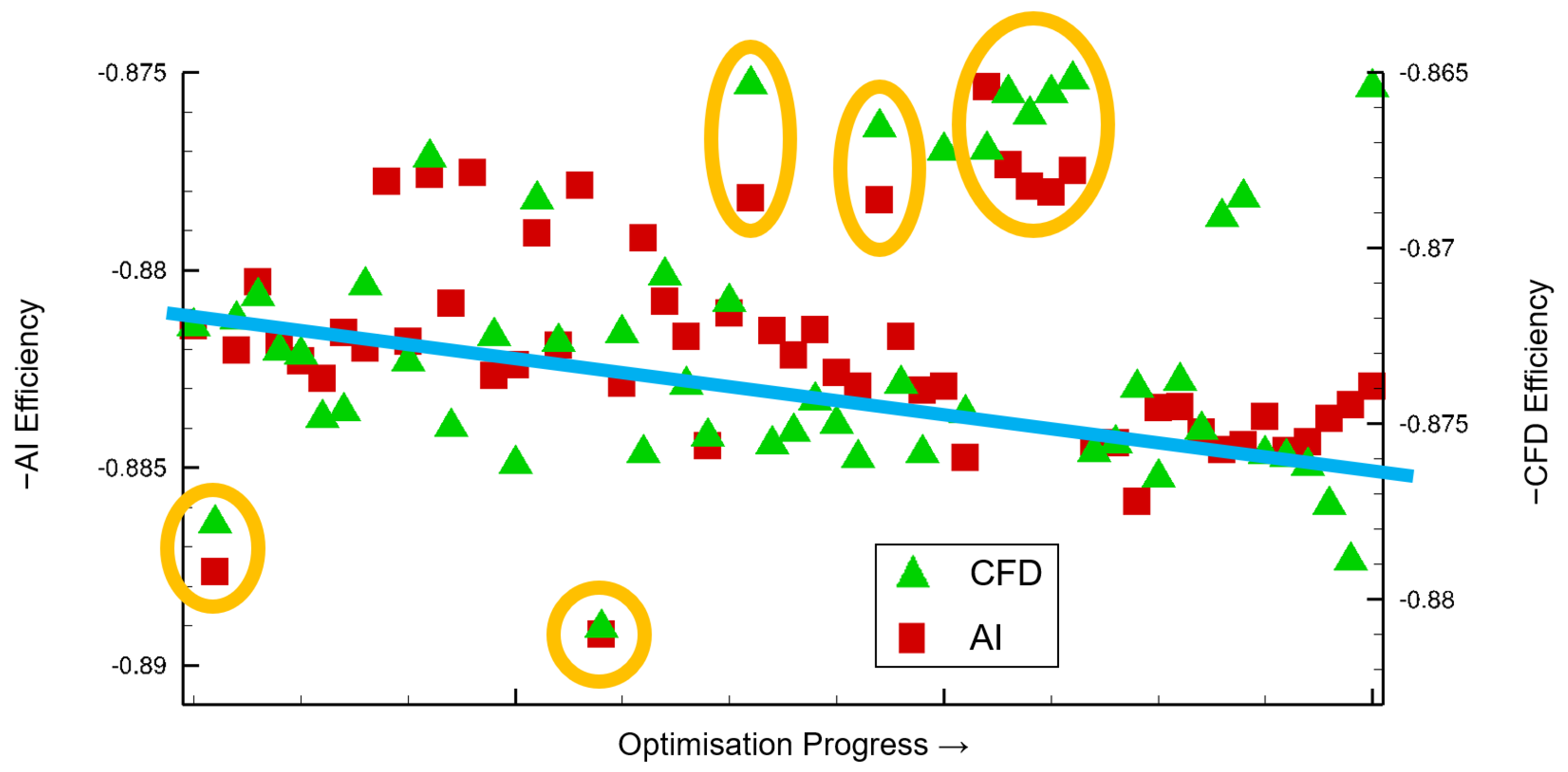
Within an optimization, however, the absolute values of the designs are of less interest. It is more important that the relative position of the designs to each other in the objective function and constraint space matches and thus the ranking remains correct. Accordingly, in order to be able to superimpose the efficiencies, it is necessary to determine the efficiencies on different axes for the AI and CFD (
Figure 18). Furthermore, the figure was magnified to provide a more comprehensive overview, with only the second half of the generated designs displayed.
The general trend of increasing efficiency during that phase in the CFD optimization is also reflected in the AI recalculations, indicated by the blue straight line in
Figure 18. In addition, most CFD “outliers”, circled in orange with their corresponding AI recalculations can also be identified. It can be posited that although the discrepancies in the efficiency target function are considerable, crucial information in the CFD database is also contained in the AI recalculations. The error in the AI approximations is primarily a general bias. Consequently, the quality of the designs, as determined by the Pareto rank, is largely preserved in the AI approximations. A comparability of the designs is, therefore, given. This has a lot of potential for accelerating the optimization. For example, a Pareto rank criterion could be specified based on AI approximations to reduce the complex validations through CFD simulations. It could be required that the designs shown in
Figure 18 must have rank 1 in the AI Pareto rank determination. In that case, only the two outliers at the bottom left would have been validated by CFD simulations. All other CFD simulations would have been omitted without a design being wrongly sorted out. The time and computational savings would be enormous.
However, this criterion only applies because of the two outliers. In general, the determination of the Pareto rank by the AI model is not accurate enough to use such a strict criterion. Therefore, a Pareto rank criterion would have to be chosen as a compromise. On the one hand, as many less promising designs as possible should be sorted out. On the other hand, no designs should be wrongly sorted out. In the database shown in
Figure 18, however, a less strict criterion would also have led to great time and computational cost savings.
In the second study, designs were generated in the optimization setup using the AI model as a CFD replacement. This is of course the toughest test for the model, as it optimizes for small total pressure increases and total temperature decreases at the compressor outlet and thus, the optimizer can move into unknown regions of the design space for which the model has not been trained. But by using the model in this way, the time and computational savings would be maximized. However, this requires an AI model that accurately represents the CFD process in a quantitative manner.
The recalculation of 100 AI-based designs in the second optimization revealed that the optimization is convergence-driven. This means that many designs do not have a solution in the CFD simulation. These designs fail in the process chain. On the other hand, the AI model always generates a flow approximation, even for unphysical boundary conditions. This means that major design changes can be made without violating the success of the process chain. The designs are no longer bound to the design space in which the CFD simulations converge. This results in only 8 of the 100 AI-generated designs having a converged solution in the CFD simulation. It is probable that the eight converged designs exhibit greater design variations than the training database, which would necessitate an extrapolation of the AI model.
Figure 19 shows a flow comparison between an AI-optimized design and CFD recalculation.
It is noticeable that the deviations are greater than in the reverse case, the comparison between CFD design and AI recalculation (
Figure 13). These deviations are not particularly noticeable at a specific point but are distributed across the flow field. The entire shock system is blurred. Details are hardly reproduced. This underlines the assumption that major design modifications have been made and the training database does not sufficiently represent these variations.
6. Discussion
The present paper demonstrates that the AI model can learn from CFD simulations that have already been carried out and transfer this knowledge to a newly parameterized optimization. In the AI recalculations of the hundred first optimization designs of a CFD optimization, the trend and some outliers of the optimization database could be reproduced in terms of integral performance parameters. For this purpose, the efficiency, a particularly sensitive target function that reacts sensitively to flow changes, was analyzed. In the opposite case, an optimization-based solely on AI as a CFD replacement, the weaknesses of the AI approach were identified. For example, AI designs were generated for which the CFD simulation did not find a solution. For an optimization that suffers from convergence problems in the CFD process, further measures should be taken to counteract this. For example, a similar problem arose when generating the training database for the AI model. Here, the design generation was based on a through-flow method, which also generated designs that did not converge in higher-order recalculations. This was countered with restrictions on deviations from individual CFD recalculations. Such a procedure could also be a possibility for the usage of the AI model during optimizations. The second optimization also showed that the effects of major design changes could not be adequately reproduced by the AI model. A larger training database with more diverse design variations should help here. This should make the AI model generally more robust with regard to design changes within optimizations.
7. Conclusions/Outlook
The successful transformer architecture could be transferred to an AI model for approximating 3D flows. This leads to the fact that the memory and computational requirements of the AI model do not directly depend on the CFD grid. Thus, the AI model can be trained with very large CFD meshes of various topologies and provide approximations. For this purpose, a complex use case was chosen that demonstrates the ability to process large CFD grids. Furthermore, this use case shows that the AI model is able to process a comprehensive setup consisting of geometry and boundary conditions. Thus, the same AI model is capable of providing approximations for a variety of compressor configurations. The structure of the AI model, which includes a module for individual blade rows, helps with this. The functionality of this model was demonstrated using the multi-stage use case. This module can be applied to the individual blade rows of different compressors to increase the generalization capabilities of the AI model.
The AI model is currently undergoing analysis and improvement in other ongoing projects. A multi-fidelity approach, in which the AI model serves as a low-fidelity process, is being considered. Furthermore, the flexibility of the AI model is being enhanced: The same AI model can be utilized for a diverse range of compressors, fans, and even industrial blowers including a far-field. Further work is being conducted on the AI model with the objective of integrating it into applications across various subject areas.
