1. Introduction
The term “aerodynamic loading”, which is widely discussed in turbomachinery, can be further divided into stage loading and blade loading. Stage loading shows the capacity of energy transformation in a stage, which is often confirmed by the change in enthalpy and is normalized by the square of the rotational speed, namely,
, where
U can be chosen as either the speed at the blade tip or the mid-span [
1]. The concept of blade loading is a little bit more complex, encompassing the blade spanwise loading and blade-to-blade (B2B) loading, where the latter, B2B loading, is the main interest of this paper.
When referring to B2B loading in more detail, the dimensionless number, the Zweifel coefficient (
) [
2], is often introduced in turbines to measure the magnitude of the circumferential force or tangential force on a blade, and the force is normalized by an ideal force composed of the product of the ideal outlet dynamic pressure head and axial chord length [
3]. The application of
is indeed closely linked to various design considerations in turbomachinery. For instance, it plays a vital role in determining the optimal solidity or the choice of the blade number, which influences the overall performance of the turbomachinery system [
2,
4,
5,
6]. Moreover, the correlation between losses and the choices of inlet and outlet flow angles is an essential facet of turbomachinery design. By considering different flow angle configurations, designers can evaluate the resulting losses within the system. The utilization of
aids in determining suitable flow angle combinations that minimize losses, enhancing the performance and efficiency of the turbomachinery design [
7].
In academia,
is a standard for research when measuring the influence of loading on a blade [
8,
9]. Additionally,
is widely employed in the literature [
5,
10,
11,
12] to describe B2B loading, as it directly originates from the definition of airfoil loading in external flow [
13].
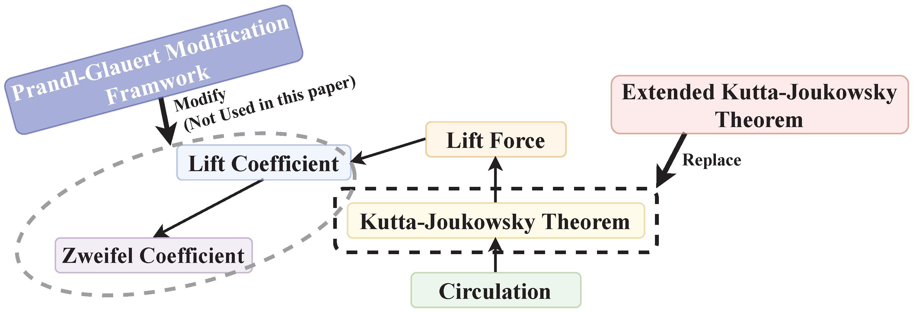
Figure 1 depicts the knowledge domains associated with
and
, illustrating the interconnected relationships between their concepts and definitions. This visual representation shows that the lift force originates from the circulation around the blade. Additionally, by employing the Kutta–Joukowski theorem, the lift forces acting on the blade can be precisely calculated. The lift coefficient, a dimensionless quantity, quantifies the lift force generated by the blade. Significantly, the Zweifel coefficient exclusively considers the circumferential force component, making it a special case of the lift coefficient.
Historically, numerous studies on B2B loading have relied on the incompressible hypothesis, which assumes equal axial velocities at the inlet and outlet. This simplification facilitated the computational process and definition [
14,
15]. However, with the growing demand for and development of highly loaded turbines aimed at reducing the number of stages, weight, and cost of modern gas turbine engines, the velocity and temperature differences between the inlet and outlet of a turbine stage have increased significantly. However, there are currently few studies that provide a specific distinction for
at high and low speeds. The incompressible assumption can introduce deviations in calculating the actual loading coefficient, leading to an overestimation of the turbine’s loading when using incompressible flow calculations for B2B loading. The specific reasons for this overestimation will be analyzed in subsequent sections.
In order to address the existing research gap about the influence of gas compressibility on B2B loading, many researchers have investigated and explored potential solutions. The current progress made for addressing this issue is summarized in
Table 1, and the comments and differences among them will be further discussed in the later part of this paper. Glassman [
16] conducted modifications on the incompressible
based on the critical velocity ratio relationship. Moustapha et al. [
17] defined a rotor blade
and performed single-stage turbine performance experiments with
ranging from 0.77 to 1.18. Song et al. [
18] provided a modified
with aspect ratio correction, which acts as one of the parameters in the tip leakage flow model. McQuilling [
19] considered the differences in inlet and outlet velocities and provided a modified definition of
, thereby establishing a quantified standard definition for high-lift turbine blade profiles. Gier et al. [
20] observed and emphasized that
only partially considers the compressibility effects. When
is used to evaluate blade loading, caution must be exercised. Gier also proposed a modification to the compressibility effects on
and provided a revised definition formula incorporating inlet and outlet axial velocities and areas. Coull et al. [
8] introduced a dimensionless coefficient called the circulation coefficient (
), which is defined as the ratio of the actual circulation to the ideal circulation on the blade surface, and the value of
is always smaller than
. Babajee et al. [
21] employed a direct formulation of
and compared the cases of
= 0.95 and 1.46 to investigate the laminar separation-induced transition on the turbine airfoil. Schmitz et al. [
22] employed an implicit form to calculate the blade circumferential force to calculate the compressible
and verified the performance of a low-pressure turbine stage with loading parameter
and
. Yang et al. [
23] utilized the isentropic velocity coefficient to describe the acceleration and deceleration distribution along the suction and pressure surfaces of the blade profile to calculate
. Cardamone [
24] introduced a modified formula that takes into account variations in inlet/outlet height and gas compressibility to assess the aerodynamic performance of three different turbine cascades at high-subsonic condition. Schobeiri [
5] introduced a definition of the generalized lift–solidity coefficient, considering the radius and the meridional velocity changes, to quantify the blade loading in both axial-flow and radial-flow turbomachinery.
In conclusion, the efforts shown above can be simply divided into two main categories following the traditional aerodynamic modification framework:
The intermediate method (IM): This method involves modifying the blade forces directly, offering a means to manipulate the aerodynamic performance. It offers advantages such as providing more accurate blade force calculation but also has certain limitations that need to be noticed and addressed, such as the constant density assumption.
The post-processing method (PM): This approach involves modifying the coefficient itself directly and operates within the Prandtl–Glauert modification framework. It provides a more comprehensive means of adjusting the overall characteristics of B2B loading but might have limitations in terms of accuracy and applicability under higher flow speed, especially in the transonic flow regime.
In this paper, an alternative modification will be presented under the IM approach. This modification revolves around extending the traditional incompressible Kutta–Joukowski equation into the compressible flow regime, focusing on enhancing the blade force calculation. The development of the compressible inviscid Kutta–Joukowski equation was initiated by Kasahara in 1955 [
25], laying the foundation for this research study. By exploring the compressible flow domain and utilizing an extended Kutta–Joukowski equation, enhancing the understanding and manipulation of blade forces while addressing some limitations associated with traditional approaches is anticipated. The modification in this paper can offer potential enhancements for future turbomachinery design and performance.
4. Results and Discussion
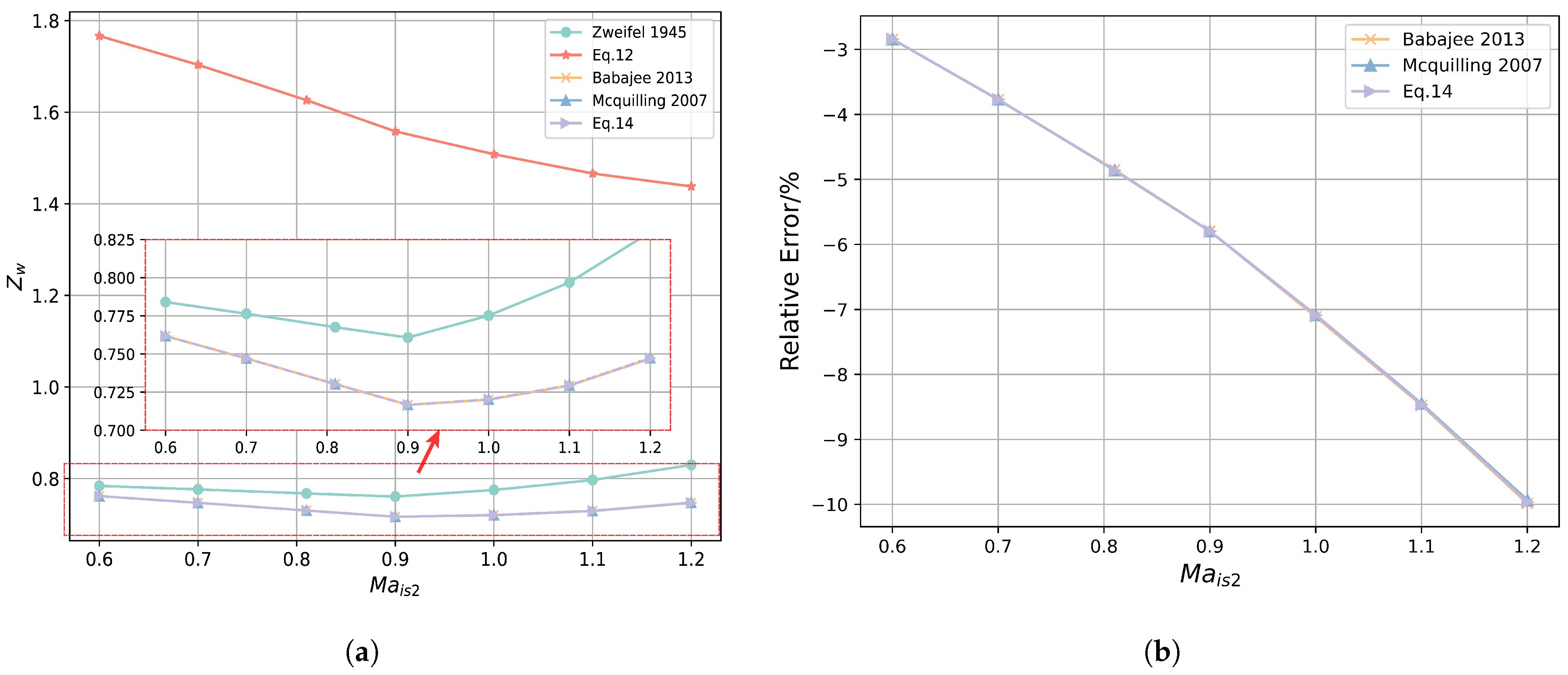
Figure 7 presents a comparative analysis of various
calculation methods and their relative errors, highlighting the impact of compressibility and input parameter choices.
Figure 7a illustrates how
varies with the isentropic outlet Mach number (
) for five distinct methods: (Zweifel 1945), (Babaejee 2013), (McQuilling 2007), and Equations (
14) and (
16). While all methods show a decreasing trend in
as
increases, Equation (
14) consistently yields the highest values. This difference stems from its unique normalization approach: Equation (
14) utilizes the averaged dynamic pressure head, while the other methods employ the outlet dynamic pressure head, which is generally larger and results in lower normalized
values.
Figure 7b focuses on the relative error of three methods—(Babaejee 2013), (McQuilling 2007), and Equation (
16)—compared with a baseline method, (Zweifel 1945). The relative error, calculated by using Equation (
20), becomes more pronounced with the increase in
for all three methods. This trend underscores the growing deviation from the incompressible (Zweifel 1945) method, as compressibility effects become more significant at higher Mach numbers. Notably, all three methods consistently produce lower
values than (Zweifel 1945), indicating that incorporating compressibility modifications leads to a reduction in the predicted Zweifel coefficient. The near-identical relative errors observed across the three methods further validate the accuracy and robustness of the proposed compressibility corrections.
The choice of the calculation method also involves considering the trade-off between simplicity and accuracy, particularly at high speeds. The incompressible (Zweifel 1945) method, requiring only and , is straightforward but less accurate at high Mach numbers. In contrast, (McQuilling 2007) necessitates four input variables (, , and inlet/outlet axial velocities), while (Babaejee 2013) demands six (inlet/outlet densities, axial velocities, and tangential velocities).
Equations (
14) and (
16) strike a balance by utilizing four parameters (
,
,
, and
), aligning with (McQuilling 2007) in terms of data acquisition complexity. Importantly, they achieve this without introducing difficult-to-obtain parameters, making them practical choices for accurate
calculations, especially in high-speed scenarios.
Furthermore, Equation (
16) exhibits good compatibility with existing empirical guidelines for selecting
values due to its use of a conventional non-dimensionalization approach. In contrast, Equation (
14)’s different non-dimensionalization reference results in a numerical range that deviates from established empirical data. However, Equation (
14) is particularly well suited for airfoil similarity studies because it derives both blade forces and the non-dimensionalization baseline from a weighted average of inlet and outlet velocities, providing a more physically representative model of flow conditions and blade loading.
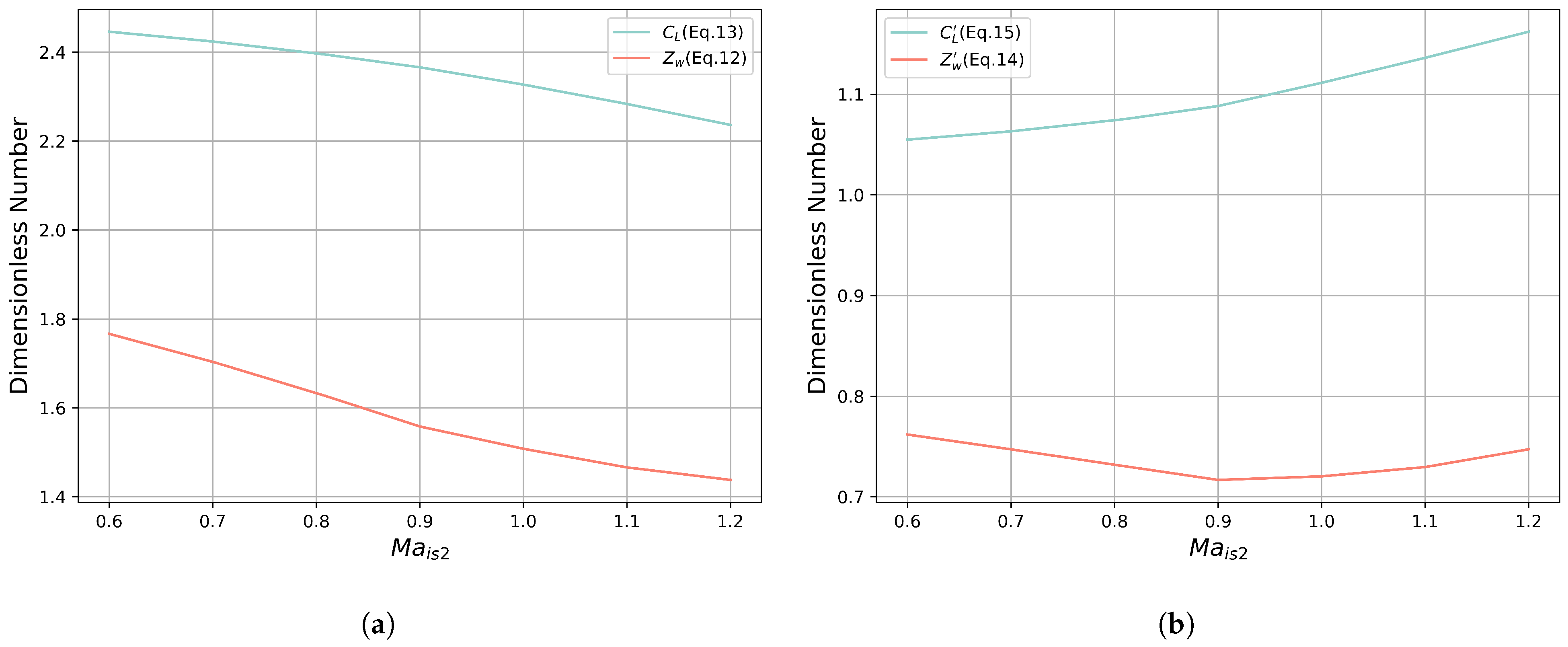
Figure 8 presents a comparative analysis of the trends exhibited by
and
for different
, calculated by using two distinct sets of equations.
Figure 8a,b illustrate the contrasting trends of
and
calculated by using average-state and outlet-based definitions, respectively.
Figure 8a shows both
(Equation (
15)) and
(Equation (
14)) decreasing with the increase in the outlet isentropic Mach number (
), with
being consistently higher than
. This trend aligns with fundamental flow physics: as
increases, local supersonic regions and shock waves may emerge on the blade surface, introducing shockwave drag. This shockwave drag is a pressure drag, effectively reducing
and
.
While
Figure 8b shows
(Equation (
17)) increasing with
, the trend for
(Equation (
16)) is less pronounced than in
Figure 8a, making it less suitable for analyzing the influence of compressibility on blade loading.
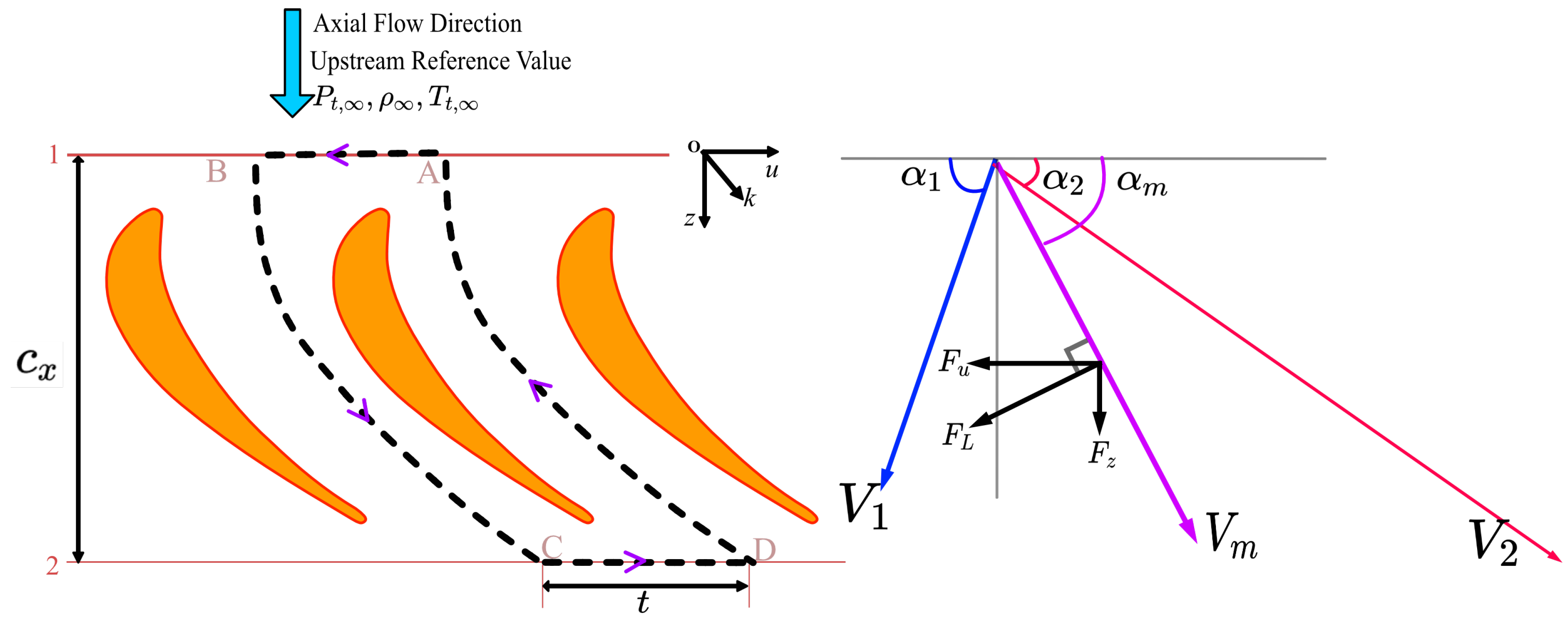
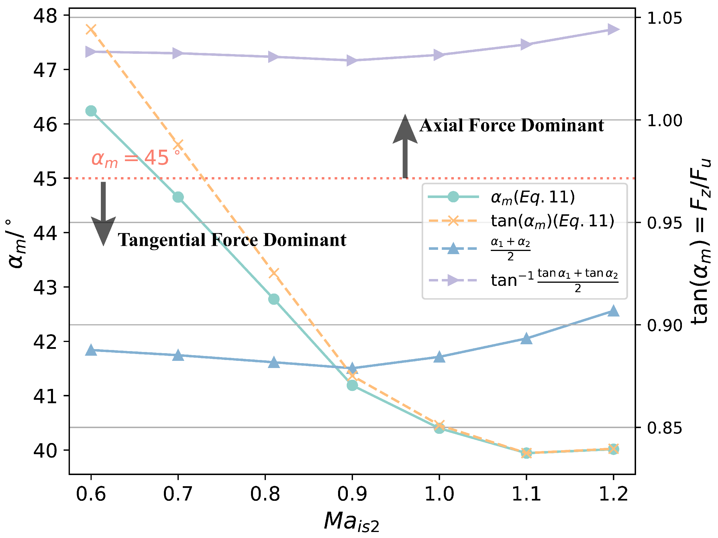
Figure 9 illustrates the relationship between the averaged flow angle (
) and the isentropic Mach number at the outlet plane (
), comparing different calculation methods. The light-blue line with circular markers represents the variation in
with the increase in
calculated by using Equation (
13), while the orange dashed line with x markers shows the corresponding trend of
, also derived from Equation (
13), which represents the ratio of axial force (
) to tangential force (
). As the outlet Mach number increases, the averaged flow angle decreases, indicating a shift in flow direction towards a more tangential orientation. However, the rate of decrease in
slows down as
increases.
Two additional methods for determining the averaged flow angle linearly are presented. The blue line with triangular markers represents a simple arithmetic average of the flow angles at inlet and outlet, denoted by (
); it remains consistently below 45° across all
, suggesting axial force dominance throughout. Conversely, the purple line with arrow markers, representing the averaged flow angle calculated by using the arctangent function (
), stays above 45° for all
, indicating tangential force dominance. These two methods, while similar in trend, exhibit an increasing averaged flow angle as the outlet Mach number increases, contrasting with the decreasing trend observed for the methods based on Equation (
13).
These contrasting trends highlight the significant influence of the averaging method, particularly the inclusion or exclusion of velocity weighting, on the flow angle and the resulting interpretation of force dominance.
The velocity-weighted approach of Equation (
13) appears to capture a more agreeable and potentially more accurate representation of the flow physics, revealing a transition in force dominance that is not apparent in the non-weighted methods. This finding underscores the importance of carefully considering the averaging method and its underlying assumptions when analyzing flow angles and inferring force characteristics, especially in scenarios with varying Mach numbers.
Based upon the preceding discussion, a strict set of similarity criteria for blade modular design are proposed, encompassing three primary aspects:
Mach number-based velocity similarity: This criterion ensures that the flow velocities are scaled appropriately between the model and the real blade, maintaining similar compressibility effects.
Blade surface pressure distribution similarity: This criterion emphasizes matching the pressure distribution on the blade surface, either through the isentropic Mach number or the pressure coefficient. This ensures similar aerodynamic loads acting on the blade.
Averaged flow angle-based blade force similarity: This criterion ensures that the overall force vectors acting on the blade are scaled proportionally between the model and the real blade. This can be achieved by matching the averaged flow angle (
). Notably, as demonstrated in Equation (
18), this criterion is interchangeable with simultaneously satisfying the similarity of both the Zweifel coefficient (
) and the lift coefficient (
). This interchangeability arises because the ratio of
to
is solely a function of
.
