Article

Brushless DC Motor Sizing Algorithm for Small UAS Conceptual Designers

Department of Aerospace Engineering, Texas A&M University, College Station, TX 77840, USA
*
Author to whom correspondence should be addressed.
Aerospace 2024, 11(8), 649; https://doi.org/10.3390/aerospace11080649
Submission received: 16 July 2024 / Revised: 8 August 2024 / Accepted: 8 August 2024 / Published: 10 August 2024
(This article belongs to the Special Issue Aircraft Design (SI-6/2024))

Abstract

:
Accurately sizing vehicle components is an impactful step in the aircraft design process. However, existing methods of sizing brushless DC (BLDC) motors for small unmanned aerial systems (SUAS) ignore how cooling affects motor size. Moreover, the literature methods do not predict a notional motor’s electrical constants, namely winding resistance, torque constant, and figure of merit. We developed a sizing algorithm that predicts the optimal mass and electrical constants using a combination of sizing, efficiency, and thermal models. The algorithm works for radial-flux BLDC motors with masses up to 800 g. An experimental teardown of seven motors informed the algorithm’s sizing models. The teardown motors varied in mass (24–600 g) and geometry (stator aspect ratio of 1.4–9.0). Validated against an independent catalog of 30 motors, the sizing models predicted mass and resistance within 10% and 20% of catalog specifications, respectively. Validated against experimental data, the full algorithm predicted mass, efficiency, and temperature within 20%, 5%, and 10% accuracy, respectively. The algorithm also captured how lowering mass would increase losses and temperature, which the literature models ignore. The algorithm can help users develop more viable concepts that save costs in the long run.

Graphical Abstract

1. Introduction

The motor sizing modules in today’s small UAS design tools do not account for a motor’s thermal dynamics. Existing methods typically use a constant specific power or specific torque metric to estimate mass from power or torque, respectively, as depicted in Figure 1a [1,2,3]. In the process, they ignore the nuances of motor physics and overlook how cooling can drastically affect a motor’s specific torque and power ratios. Existing tools also do not estimate the key electrical constants of notional motors, such as winding resistance ( R m ) and torque constant ( k t ). Conceptual designers need these parameters to estimate motor losses and power draw [4,5], which then inform battery sizing and vehicle performance calculations.
Our goal was to address the knowledge gap with respect to the sizing of brushless DC motors (BLDC) in the literature on small UAS design. The challenge was to (1) bridge the gap between ideal theories that relate torque to volume—but not mass—and (2) account for the extrinsic thermal response of notional motors in arbitrary environments. Our solution is an iterative algorithm rather than a direct function, which can predict motor mass, geometry, and electrical constants for conceptual designers at the early design stage. The core of the sizing algorithm is a physics-based sizing expression that relies on temperature feedback from previously developed efficiency and thermal models. A parametric experimental teardown of different BLDC motors informed empirical and semi-empirical regressions that supplement the idealized physical sizing expression.
Our objectives for this study were to (1) deconstruct and study the mass and geometric variations of standard BLDC motors, (2) develop empirical and semi-empirical regression models from the teardown data, (3) validate the regression models against an independent set of motor data, and (4) provide guidance on how to abstract our approach to size other electric powertrain components, such as the motor controller.
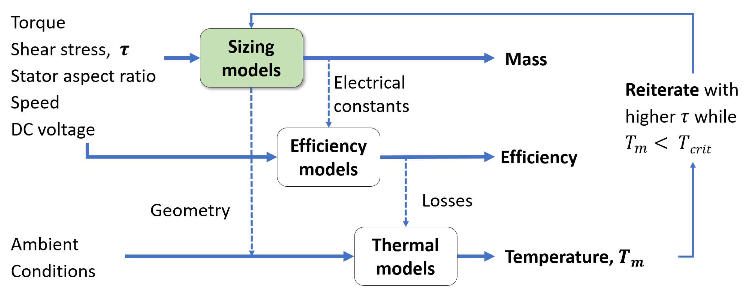
Figure 1b depicts our thermally informed algorithm. Unlike the literature methods, our method progressively sizes smaller and smaller motors and evaluates the thermal response of each design in the specified environment. The algorithm uses a combination of sizing, efficiency, and thermal models that are discussed later. The penultimate iteration yields the optimal motor for a given load and operating environment. The algorithm also predicts the motor’s electrical constants for each iteration. Finally, the intermediary iterations are also valuable to conceptual designers because these data can inform higher-level optimization studies. For example, a slightly larger motor might operate more efficiently and require a smaller battery over a more extended mission.
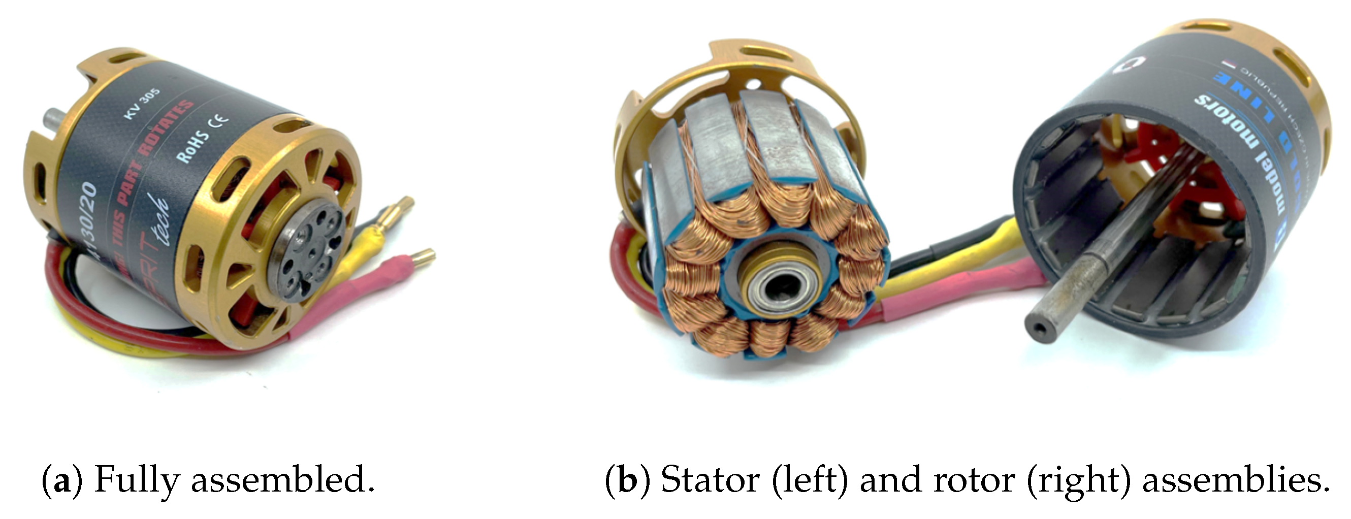
The sizing algorithm applies to outrunner brushless DC (BLDC) motors up to 800 g in mass that experience axial air cooling. Motors such as that pictured in Figure 2 are commonly found in fixed-wing small UAS driven by an open propeller or an electric ducted fan (EDF) [6,7]. The sizing algorithm is especially suited for EDF applications wherein the high-velocity axial flow can provide excellent cooling to reduce a motor’s size and mass. In the electric machine literature, outrunner BLDC motors are known as radial-flux outer-rotor permanent magnet synchronous motors (PMSMs). The algorithm does not apply to other motor topologies such as inrunner BLDCs or axial-flux motors because these other motors are less commonly found in small UAS and have fundamentally different constructions.
This research contributes to the state of the art through the presentation of analytical models and parametric experimental data despite these limitations. The sizing algorithm distinguishes itself from other methods because it accounts for how cooling drives motor size. The experimental data distinguish themselves from other literature data because they explore the mass and geometry variations of a range of motors rather than a single-point design.
Practitioners and researchers can apply our sizing algorithm to design more weight-optimized small UAS. The algorithm relies on thermal-in-the-loop modeling to iteratively find the minimal-mass motor that delivers the required torque. This feature can benefit conceptual designers by reducing the number of costly design revisions later in a vehicle’s development timeline. Users can re-tune our equations for other motor topologies or apply our broader approach to develop sizing algorithms for different components, such as the motor controller.
Practitioners and researchers can use the experimental data to understand motors better and develop sizing models. Motor designers can use the experimental data as a reference point to validate new designs. The experimental data can even inform modeling beyond motor sizing, such as transient thermal modeling. Multi-body thermal circuit models for motors require mass data for constituent components such as the stator, rotor, and bearings. These data are impossible to collect without acquiring and physically tearing apart a motor [8].

1.1. Motor Primer

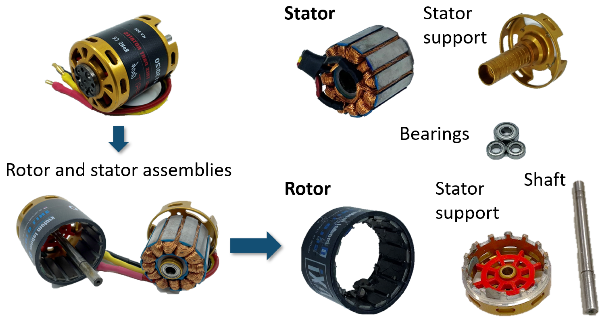
A brushless DC motor consists of two assemblies, namely a stationary stator and a rotating rotor, as shown in Figure 2. The stator consists of a steel core with radial spokes (or teeth, as they are known in the motor design literature). Each tooth is wound with copper wire and is an electromagnet (winding). The stator assembly also contains bearings and a rotating shaft fixed to the rotor. The rotor is a circumferential array of discrete permanent magnets. Aluminum structures support the stator and rotor [9].
A motor converts electrical power in the stator to mechanical power out of the rotor via magnetic interactions between the stator and rotor. Current (I) enters select stator windings and generates a magnetic field around the stator. The rotor magnets seek to align with the stator field, and the resulting magnetic forces act as net torque (M) on the shaft that spins the rotor. The motor controller constantly cycles power through different windings to revolve the stator’s field ahead of the rotor field, thereby maintaining output torque [10]. The magnetic interactions also induce a back-electromotive force (or back-EMF, V E M F ) inside the windings that opposes the motor controller’s supply voltage [11].
Three key electrical constants define a motor:
1.
Torque constant ( k t ) is the slope of the linear region in a motor’s torque–current curve, as expressed in Equation (1). As such, k t is analogous to a wing’s lift curve slope ( c L α ). The torque constant also relates the motor’s back-EMF ( V E M F ) to its rotational speed ( ω ), as expressed in Equation (2).
M = k t I
V E M F = k t ω
2.
Winding resistance ( R m ) is, as the name implies, the resistance of the motor’s windings to the current flow. The winding resistance is roughly analogous to an aerodynamic body’s parasitic drag coefficient ( c D 0 ).
3.
Motor figure of merit ( k m ) quantifies how well a particular motor’s design converts current into torque rather than copper losses ( P C u = I 2 R m ), as defined in Equation (3). The figure of merit is roughly analogous to a wing’s lift-to-drag coefficient ( L / D ).
k m = M P C u = k t I I 2 R m = k t R m

1.2. Literature Review

The motor design literature shows that the available cooling and the required torque drive motor size. Equation (4) expresses a motor’s output torque (M) as a function of the electromagnetic shear stress ( τ ) and the ideal volume ( U i d ). The shear stress is a measure of the electromagnetic loading that a motor can generate. The primary limit to shear stress is the motor’s ability to dissipate the resulting losses [12,13] via cooling. The ideal volume is the motor’s theoretical minimum footprint. For outrunner BLDC motors, the ideal volume is approximately the stator’s footprint ( U S F P ), which is expressed in Equation (5) as a function of the stator’s diameter ( D s ) and length ( L s ).
M = 2 τ U i d
U i d U S F P = π 4 D s 2 L s
A motor’s aspect ratio also influences torque output. Motor designers define aspect ratio as the ratio between the stator’s diameter and length ( A R s , Equation (6)). High-aspect-ratio motors, which are like thin discs ( D s > L s ), have large moment arms through which the magnetic forces between the stator and rotor generate torque. Therefore, high-aspect-ratio motors can generate more torque per unit current (higher k t ) and are commonly found in direct-drive applications, such as driving small UAS propellers. Low-aspect-ratio motors, which are like long tubes ( L s D s ) , have smaller rotational inertias and are optimal for geared applications, such as powering ground robot drivetrains.
A R s = D s / L s
Existing aircraft design tools incorrectly use specific power to size motors [3,14,15,16]. These approaches tabulate power and mass data for several commercial electric motors. They apply linear regression to these data and use the slope as a constant specific power metric to size notional motors. This is doubly inappropriate because (1) torque, not power, drives size, and (2) specific torque is itself a variable function of cooling, as we discuss later. A small (light) motor operating at low torque and high rotational speed can deliver as much power as a large (heavy) motor operating at high torque and low speed.
A sizing approach that relies on specific power delivers poorly sized motors and increases vehicle development costs. A specific power regressed from high-speed, low-torque motor data undersizes notional motors for low-speed, high-torque applications at constant power. Conversely, a specific power regressed from low-speed, high-torque data oversizes motors for high-speed, low-torque applications at constant power. In both instances, the sub-optimal solution would skew other systems, such as battery mass, as well as the vehicle’s overall performance. The vehicle would need costly design revisions in the detailed design or prototyping stages.
Other tools use a slightly better but still inaccurate specific torque [1,2,17,18] to size motors. Researchers have tabulated torque and mass data for several commercial electric motors, applying linear regression to these data and using the slope as a constant specific torque metric to size notional motors. This approach is still unreliable because a motor’s specific torque is a variable function of available cooling. Volumetric torque density is a variable function of cooling ( M / U i d τ per Equation (4)). Assuming mass is proportional to volume ( m U i d ), then the volumetric torque density is proportional to the gravimetric torque density or specific torque ( M / U i d M / m ). Therefore, specific torque is proportional to cooling ( M / m τ ), and cooling is an extrinsic process that depends on ambient conditions.
A sizing approach that relies on constant specific torque delivers poorly sized motors and increases vehicle development costs. A specific torque regressed from well-cooled, high-shear motor data undersizes notional motors in poorly cooled environments. Conversely, a specific torque regressed from poorly-cooled, low-shear data oversizes motors in well-cooled environments. In both instances, the sub-optimal solution would, again, skew other systems, such as battery mass, as well as the vehicle’s overall performance and development costs.
Fundamentally, these literature approaches rely on unreliable and uncertain commercial data. A motor’s power and torque ratings are functions of the ambient environment [19]. Hobbyist BLDC vendors, which supply most small UAS motors, do not usually publish torque ratings or adhere to consistent environmental test conditions [20]. Therefore, the torque and power data points that inform literature regressions are uncertain and rated with respect to unknown thermal reference frames.
The literature also lacks experimental data on the varying size and constitution of small UAS BLDC motors. Oak Ridge National Laboratory conducted in-depth powertrain teardowns of motors of popular automotive hybrid vehicles [21,22]. However, their data do not apply to small UAS motors. The brushless motor design literature offers details, such as the number of copper wire turns per winding, for different example cases. However, these low-level motor data are beyond the scope of conceptual designers. These example cases do not discuss high-level trends of mass or volume, which are particularly important to aircraft designers.
The literature would benefit from a sizing approach that incorporates—rather than ignores—the influences of temperature and geometry on motor size and mass. A nuanced, thermal-in-the-loop approach could size the optimal motor for a given environment and geometric constraints. Experimental mass and geometry measurements from a variety of small UAS motors would also help expand literature data and could inform sizing models.

2. Methodology

We pursued a combination of analytical modeling and parametric experimental studies to develop and validate a thermal-in-the-loop sizing algorithm that addresses the gaps in the literature.

2.1. Overall Algorithm

Figure 3 depicts the algorithm, which consists of a combination of analytical sizing, efficiency, and thermal models. First, the sizing model block estimates the ideal volume required to deliver a user-defined torque using an initial conservative shear stress ( τ ). Then, the sizing model block estimates the notional motor’s mass and outer dimensions, as well as the electrical constants of the notional motor. Next, an efficiency model block predicts the motor’s losses and efficiency with the user-provided loads and the sizing-estimated electrical constants. Finally, the thermal model block uses the (1) estimated losses from the efficiency block, (2) the estimated outer dimensions from the sizing block, and (3) the ambient temperature and flow conditions from the user to predict the motor’s temperature. If the predicted temperature ( T m ) is below a critical temperature ( T c r i t ), then the algorithm sizes a new motor using a slightly higher shear stress. The algorithm iterates until the notional motor’s steady-state temperature exceeds the specified thermal limit.
This paper develops and validates the sizing models, which correspond to the highlighted block in Figure 3. The broader algorithm uses our previously developed efficiency and thermal models, which are represented by the other boxed blocks in Figure 3. In reference [23], we developed the efficiency models and validated them against flight data from a flying small UAS. In reference [19], we developed the thermal models and validated them against parametric wind tunnel tests of different BLDC motors. Where relevant, we briefly discuss the key equations of the efficiency and thermal models, but readers should refer to refs. [19,23] for details.

2.2. Sizing Models

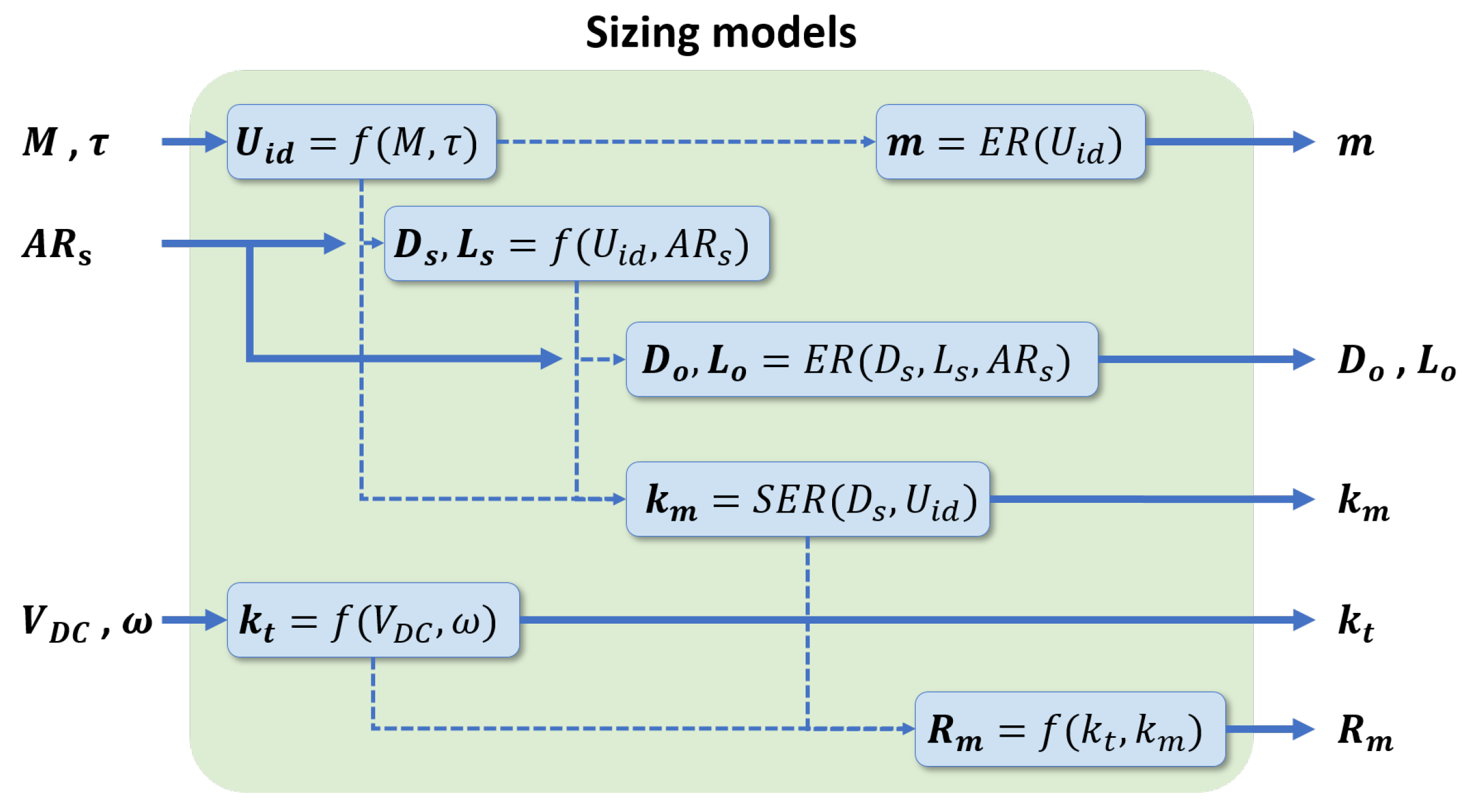
Figure 4 shows the internal sub-routines of the sizing block highlighted in Figure 3. These expressions consist of physics-based functions ( f ( x ) ), empirical regressions ( E R ( x ) ), and a semi-empirical regression ( S E R ( x ) ). First, Equation (4) sizes the motor’s ideal volume ( U i d ) from a user-provided torque (M) and conservative shear stress ( τ ). Multiplying the ideal volume by an empirically derived density yields the motor’s mass (m). Using the ideal volume and a user-provided stator aspect ratio ( A R s ), Equations (5) and (6) then yield the stator diameter ( D s ) and length ( L s ). Using the previously predicted parameters, another set of empirical regressions predicts the outer diameter ( D o ) and length ( L o ). Equation (2) and a semi-empirical regression estimate the motor’s electrical constants ( k t , R m , and k m ) from the predicted stator dimensions and user-defined voltage ( V D C ) and operating speed ( ω ).
Fundamentally, estimating mass and dimensions from the ideal volume decouples the sizing problem from the influence of cooling. A motor’s thermal sensitivity is embedded within τ , whereas U i d is a mechanical parameter. Therefore, empirical studies can safely estimate other mechanical terms, such as mass or diameter, from U i d . In contrast, the literature methods use a constant specific torque or power metric to estimate mass directly. The resulting mass prediction is still thermally coupled and should not be used to calculate other mechanical terms.
Section 3 develops the aforementioned empirical regressions. Section 4 compares the predictions of these analytical models against known specifications from an independent catalog of 30 motors. Section 5 combines the sizing models with efficiency and thermal models into the entire algorithm and compares the algorithm’s predictions obtained with other sizing methodologies in the literature.

2.3. Teardown Motors

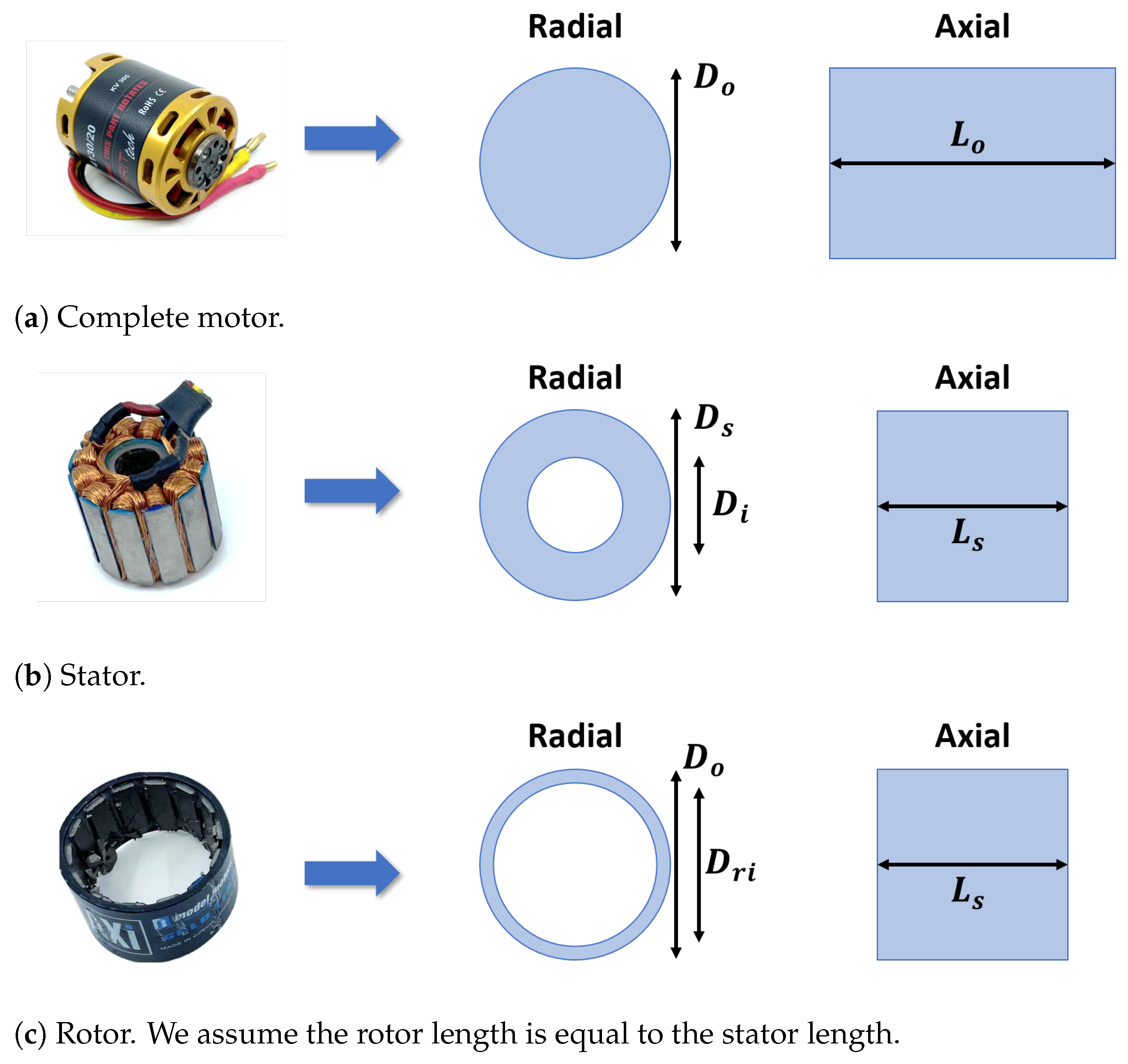
Figure 5 depicts an experimental teardown that provided parametric experimental data for the regressions shown in Figure 4. We deconstructed seven motors from four different manufacturers into their constituent components, namely stator, stator support, rotor, rotor support, shaft, and bearings. Figure 6 labels the dimensions of the most important components, i.e., the stator and rotor. Table 1 lists the values of these salient dimensions for all seven motors. The teardown motors vary in mass from nearly 25 g to 600 g and in stator aspect ratio from 1.4 to 9.0. All of the motors are outrunner BLDC motors. Apart from their aspect ratios, the motors’ most noticeable variation is in the number and shape of airflow slots in stator and rotor support components.

3. Teardown and Analysis

We present measurements and analysis from the experimental teardown of seven motors. The regressions presented in this section are used to predict motor specifications in the following section.
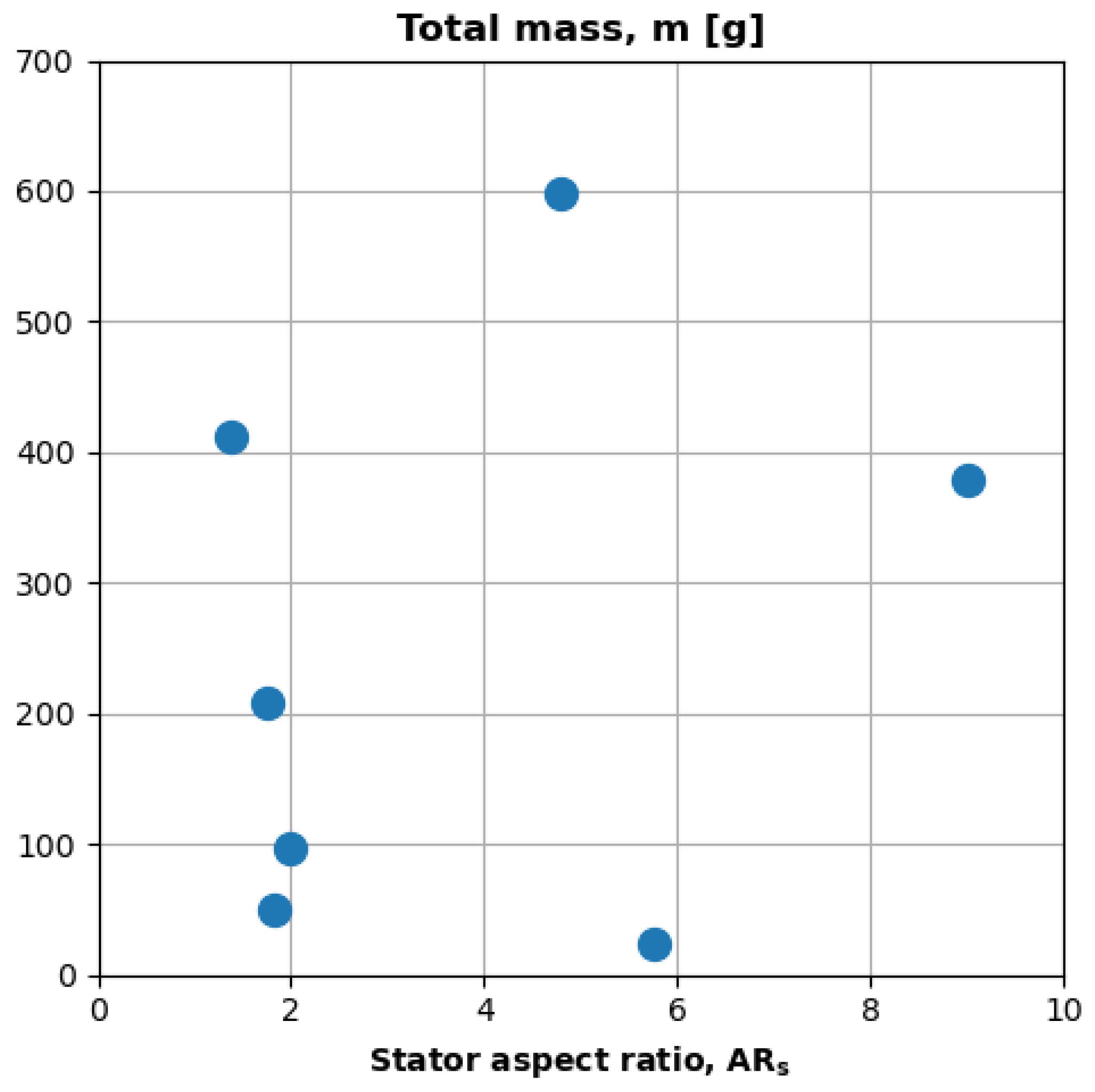
Figure 7 plots the mass and geometry of the teardown motors. The x axis is the motor aspect ratio ( A R s ), and the y axis is the total mass (m). The figure shows that the motors provide good tradespace coverage. The data contain instances where the aspect ratio is constant and mass changes ( A R s = 2, m ranges from 50 to 400; A R s 5 and m ranges from 25 g to 600 g). Conversely, the data contain two instances where mass is almost constant and aspect ratio changes ( m 37 g, A R s ranges from 2 to 6; m = 400 g, A R s ranges from 2 to 9). Low-aspect-ratio motors ( A R s 1.0) do not commonly power small UAS.

3.1. Mass Trends

Table 2 lists each motor’s constituent components’ mass fractions. The motors are numbered in order of increasing total mass ( m t o t ). The stator and rotor, the two electromagnetically active components in a motor, constitute more than 50% of all motors’ total masses. This is because these active components are made of steel and copper, which are denser than the aluminum material of the supports.
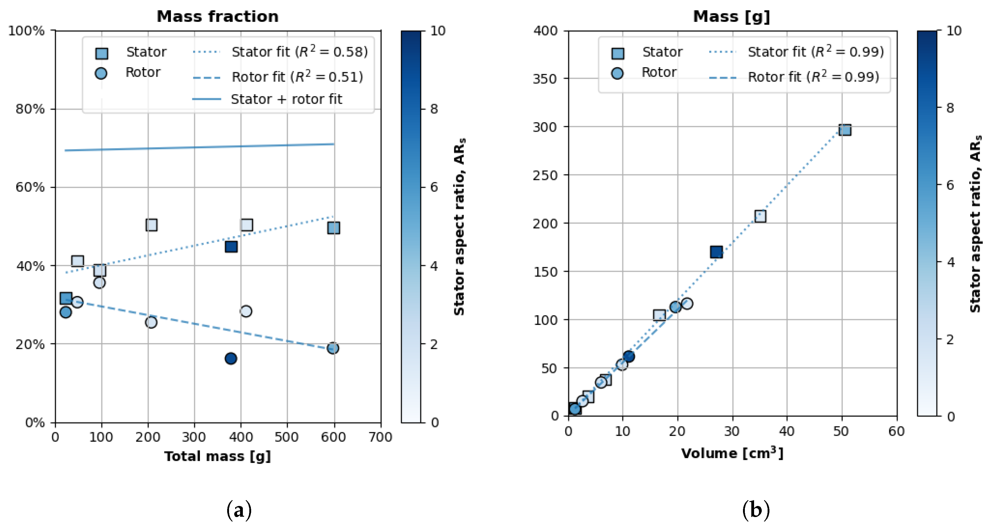
Figure 8a plots the stator and rotor mass fractions with respect to the total motor mass across the seven teardown motors. The x axis is the motor’s total mass, and the y axis is the mass-fraction percentage. The fill intensity of each data point represents the aspect ratio of the motor from which the component came. The figure also plots a linear regression of each dataset. Equations (7) and (8) are the linear regressions of the non-dimensional stator and rotor mass fractions, respectively ( w s t a t and w r o t respectively) with respect to the total mass.
w s t a t = m s t a t m t o t = 0.249 m t o t + 0.375
w r o t = m r o t m t o t = 0.210 m t o t + 0.317
Figure 8a shows that the two most active components, the stator and rotor, constitute 70% of motor mass. The stator mass fraction increases linearly with total mass, while the rotor mass fraction decreases linearly with total mass. The sum of the changing mass fractions is about 70% for all the different-sized motors. The slopes of the linear regressions (Equations (7) and (8)) are approximately equal and opposite, reflecting their diverging physical trends.
Figure 8b plots the mass versus volume of the stator and rotor. The x axis is the component’s calculated volume, and the y axis is the measured mass. The fill intensity of the data points is the aspect ratio of that component’s originating motor. Equations (9) and (10) are the equations we used to calculate the stator ( U s t a t ) and rotor ( U r o t ) volumes, respectively. Both components are cylinders with some wall thickness, as seen in Figure 5. The stator has an outer ( D s ) and inner diameter ( D i ), and the rotor has an outer ( D o ) and inner ( D r i ) diameter.
Figure 8b also plots the linear regressions of the stator mass vs. stator volume and rotor mass vs. rotor volume. Equations (11) and (12) are the linear regressions of the stator and rotor data, respectively, with a forced y intercept of zero. The slope of each equation is roughly the component’s density, and we elected to express the slope in non-SI units for practical reasons.
U s t a t = π 4 L s ( D s 2 D i 2 )
U r o t = π 4 L r ( D o 2 D r i 2 )
m s t a t = 5.97 g cm 3 U s t a t
m r o t = 5.49 g cm 3 U r o t
Figure 8b and Equations (11) and (12) show that the components both have a density of approximately 6 g/ cm 3 . The similar densities make sense because the components’ constituent elements have similar densities. The stator steel, stator copper, rotor steel, and rotor permanent magnets all have approximately the same density (8 g/ cm 3 ). Our empirical density of 6 g/ cm 3  does not match the theoretical density of 8 g/ cm 3  because the geometrically calculated volumes (Equations (9) and (10)) are approximations of the components’ actual volumes. For example, the stator volume calculation does not account for the space between the stator’s copper winding loops. Modeling the components’ geometry at such fidelity is beyond the scope of a vehicle conceptual designer.
Figure 9 plots the motor’s total mass with respect to two different volumes. The y axis is the motor’s total mass, and the x axis indicates units of volume. The triangular points are mass versus the motor’s stator footprint ( U S F P ). The pentagonal points are mass vs. the motor’s outer volume ( U o u t ). The color bar corresponds to the motor’s stator aspect ratio.
Figure 9 also plots linear regressions of each dataset. The slope of the mass–stator footprint regression (Equation (14)) is greater than the slope of the mass–outer volume regression (Equation (15)) because a motor’s stator footprint (Equation (5)) is smaller than its outer volume (Equation (13)).
U o u t = π 4 D o 2 L o
m t o t = 10.30 g cm 3 U S F P
m r o t = 2.29 g cm 3 U o u t
Figure 9 reveals that the ratio of mass to stator footprint ( m t o t / U S F P ) is more consistent than the more physically intuitive ratio of mass to outer volume ( m t o t / U o u t ). The linear regression of m t o t to U S F P has a smaller R 2 value, and we can see its superior robustness around 400 g. At this mass, one motor has an aspect ratio of less than 2, and the other has an aspect ratio greater than 8. The latter motor ( A R s > 8 ) has roughly double the outer volume of the former motor; however, their stator footprints (SFPs) are almost the same. This suggests we should use and m t o t / U S F P ratio ≈ 10.3 g/ cm 3 to estimate mass from a notional stator footprint because this quasi-density is less susceptible to variations in geometry.
The mass–SFP density (10.3 g/ cm 3 ) is greater than the density of a motor’s constitutive elements, like steel (8 g/ cm 3 ), because the SFP is smaller than the physically displaced volume of a motor. Conversely, the mass–total volume density (2.29 g/ cm 3 ) is less than the motor’s constitutive densities because the geometrically calculated total volume includes (empty) space, such as the support components’ cooling slots.

3.2. Geometry Trends

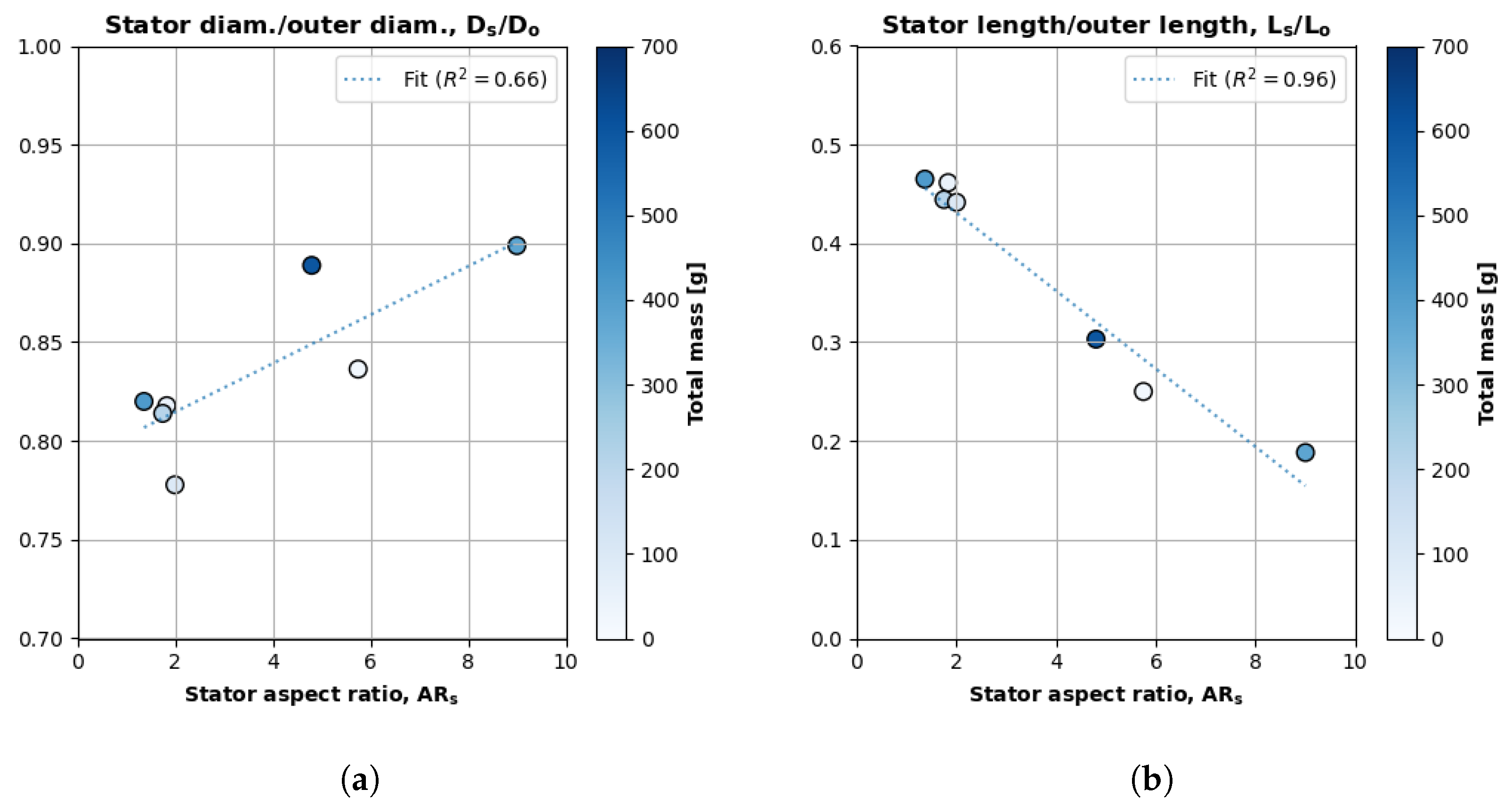
Figure 10a plots changes in the ratio of a motor’s stator diameter to its outer diameter. The x axis is the motor’s aspect ratio ( A R s ), and the y axis is the motor’s stator–diameter ratio ( D s / D o ). The fill intensity of each data point corresponds to the motor’s total mass. Figure 10a also plots the linear regression of the stator’s outer diameter ratio relative to the aspect ratio (Equation (16)).
D s D o = ( 1.23 × 10 2 ) A R s + 0.79
Figure 10a shows that the stator diameter constitutes an increasingly larger portion of the total (outer) diameter as a motor becomes wider and more pancake-like ( D s > L s ). The stator diameter is the driving factor for high aspect ratios; therefore, it makes sense that stator and outer diameter approach unity at high aspect ratios.
Figure 10b plots the ratio of a motor’s stator length to its outer length as a function of its aspect ratio. The x axis is the motor’s aspect ratio, and the y axis is the motor’s stator length versus its outer length. The fill intensity of each data point corresponds to the motor’s total mass. Figure 10b also plots the linear regression of the stator’s outer length ratio relative to the aspect ratio (Equation (17)).
L s L o = ( 3.95 × 10 2 ) A R s + 0.51
Figure 10b shows that the stator length constitutes a smaller portion of the total length as the aspect ratio increases. The stator length is the subordinate dimension in high aspect ratios; therefore, stator length plays a more minor role in the overall motor length as the aspect ratio increases.

3.3. Figure-of-Merit Trends

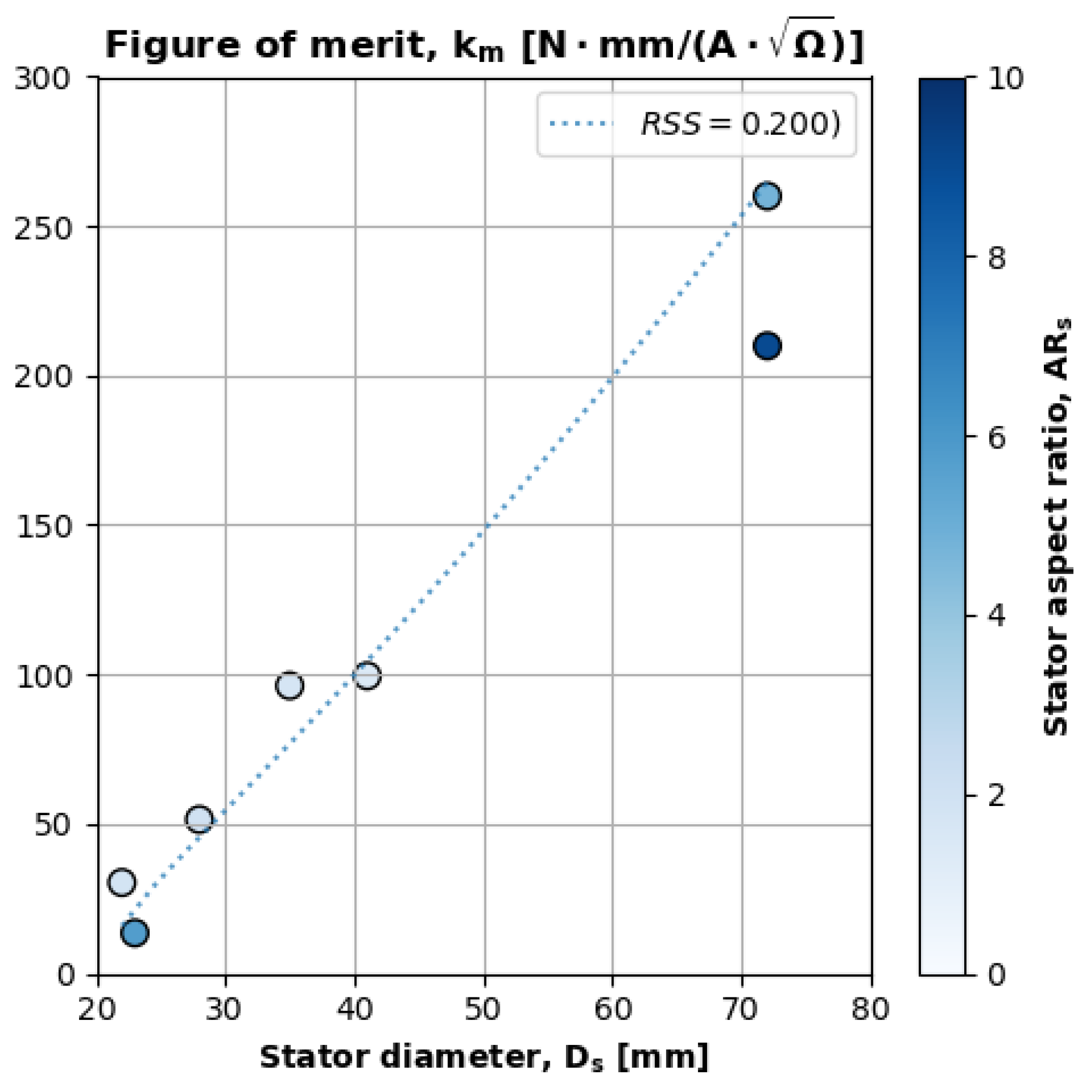
Figure 11 plots the teardown motors’ figures of merit (y axis) versus their stator diameters (x axis). The fill intensity of each data point corresponds to the motors’ aspect ratios. Figure 11 also plots a semi-empirical power-law regression, which we derive shortly. The slope of this fit line is approximately linear because theory suggests k m D s [24].
Equation (18) expresses the motor figure of merit ( k m ) as a function of motor design parameters as derived by Hanselman for radial-flux BLDC motors [24]. The figure of merit is a function of the motor’s magnetic loading (B), the stator diameter ( D s ), the volume of copper inside the motor ( U C u ), and the resistivity of copper ( ζ C u ).
k m = 1 2 B D s U C u ζ C u
Equation (18) reveals how copper volume provides some flexibility to motor designers to adjust a conceptual motor for different voltage and current applications. A notional motor with a fixed size can have windings that consist of many turns of a single copper wire. This motor has high k t and high R m and is suitable for high-voltage and low-current applications. At the same size, another motor can have windings that consist of fewer turns of multiple parallel copper wires. The second motor has low k t and R m and is suitable for low-voltage, high-current applications. In both instances, the total copper volume and the figure of merit are roughly constant.
For aluminum-wound motors, U C u and ζ C u are parameterized with the appropriate values for aluminum. The aviation industry has explored aluminum cabling because aluminum is lighter and more flexible than copper. Aluminum even has a lower resistivity per unit mass, i.e., 1 × 10 6   cm 4 Ω g vs. 1.9 × 10 7   cm 4 Ω g [25]. However, aluminum also has a higher coefficient of thermal expansion, which may lead to faster thermal failure in motors. Further discussion is beyond the scope of this paper.
We developed two semi-empirical versions of Equation (18) via power-law regression of teardown data (Equations (19) and (20)). We approximated magnetic loading and copper resistivity as constants, since they are material properties that are essentially the same for high-quality BLDC motors [26]. Equation (19) is a regression that approximates the copper volume as the stator footprint ( U C u U S F P , Equation (5)). The residual sum of squares (RSS) for this regression is 0.2. Equation (20) is a regression that more accurately approximates the copper volume as the stator volume ( U C u U s t a t , Equation (9)). The RSS for the copper–stator volume regression (Equation (20)) is 0.218. Approximating copper volume using stator volume is more physically accurate because the hollow stator volume (Equation (9)) excludes the central space occupied by the shaft and bearings.
k m = 333 D s 0.80 U S F P 0.52
k m = 319 D s 0.85 U s t a t 0.49
Surprisingly, approximating copper volume with the stator footprint (Equation (19)) predicts the motor figure of merit more accurately, since the SFP regression has a smaller residual sum of squares (RSS). The higher accuracy of the SFP approximation is also more practical for conceptual designers, since the stator’s inner diameter, which is required to calculate the stator volume, may not always be known. Otherwise, Equations (19) and (20) have similar exponents that closely match theoretical values. Hanselman’s derivation suggests k m D s , and the D s exponent in both regressions is approximately 1. Likewise, theory suggests k m U C u , and the U exponent in both regressions is approximately 0.5.

4. Sizing Models and Validation

We compared predictions from the empirical regressions developed in the previous section to specifications from an independent catalog of more than 30 motors. The catalog motors spanned a least an order of magnitude in mass (18 g to 1075 g) and stator aspect ratio (0.9 to 9.0).
We assume the stator footprint is known, since the broader algorithm iteratively solves Equation (4) for U S F P  with varying shear stress values. From the stator footprint and a user-prescribed stator aspect ratio ( A R s ), we can solve for the stator diameter and stator length via Equations (21) and (22), respectively. The user can sweep different aspect ratios in a more extensive trade study.
D s = 4 U S F P A R s π 3
L s = 4 U S F P π A R s 2 3

4.1. Mass

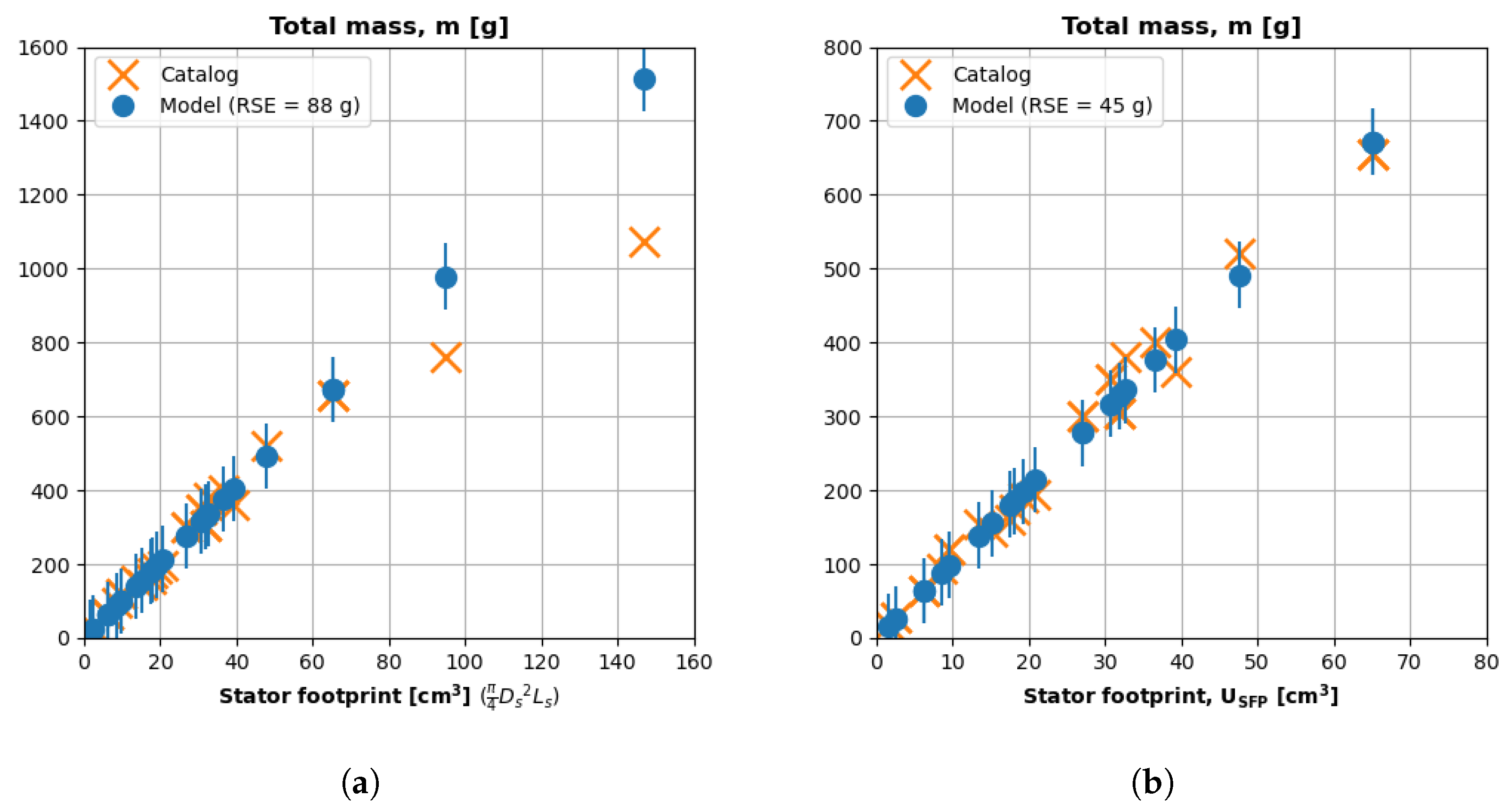
Figure 12 plots the measured and predicted mass for the motor catalog. The x axis is the stator footprint, and the y axis is the total mass. The predicted mass is the product of U S F P  and the ratio of mass to stator footprint (10.3 g/ cm 3 ) regressed in Equation (14). The predictions have a residual standard error (RSE) of 88 g, as represented by the vertical error bars on the model data points.
The mass predictions are within the error bars of the model for motors with a mass of less than 800 g and a stator footprint of less than 80 cm 3 . We suspect the mass model fails above this point because stators at this scale are more hollow and ring-like than the seven teardown motors used to tune the mass model. For example, ref. [27] points to the datasheet of the 150 cm 3 , 1 kg motor plotted at the upper-right extreme of Figure 12. Reference [28] points to the datasheet of one of our teardown motors. The 1 kg motor has a more hollow stator than our teardown motor. Our solid-biased mass model overestimates the mass of the 150 cm 3 motor by 50%.

4.2. Geometry

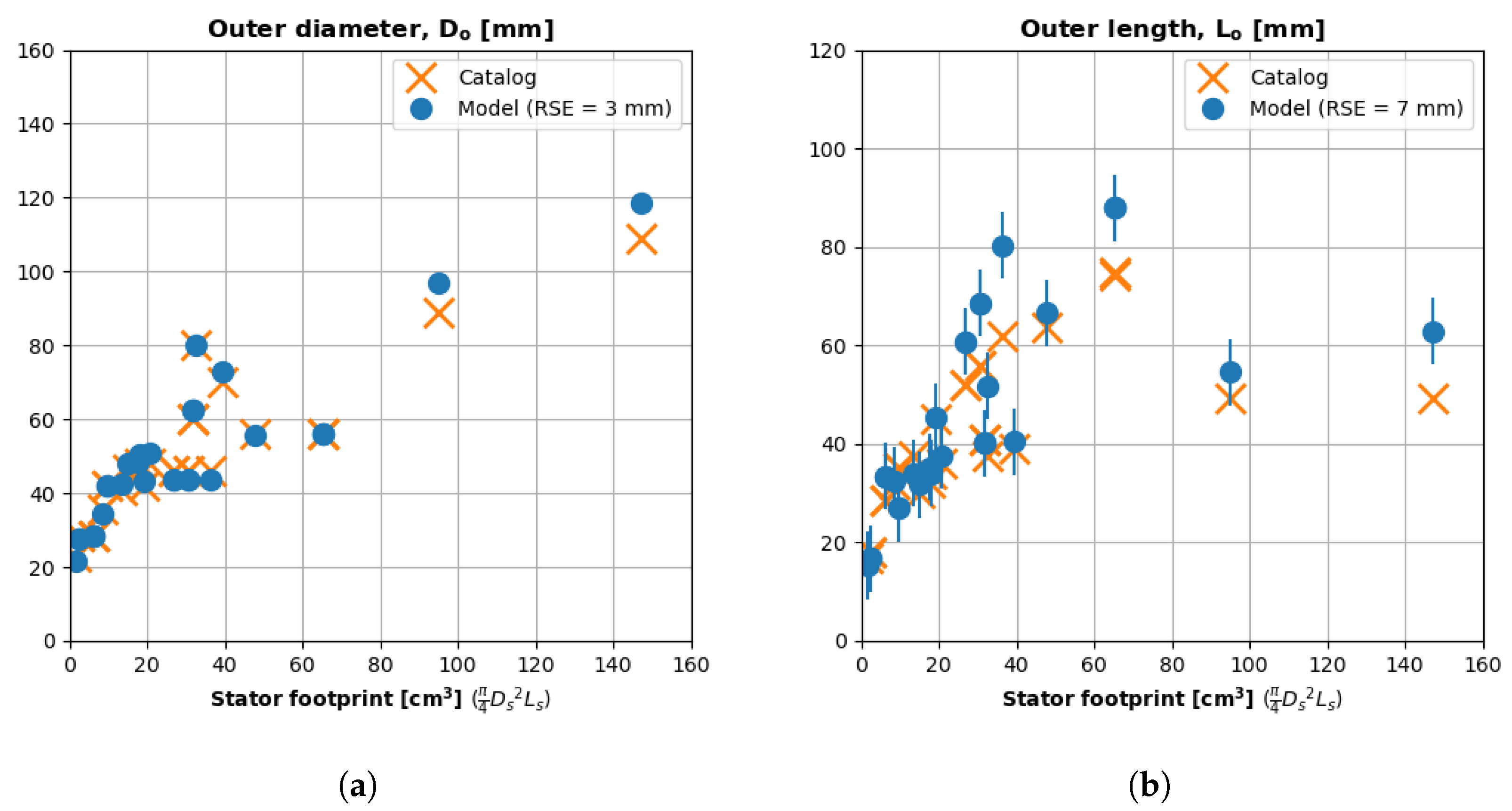
Figure 13a plots the measured and predicted outer diameters for the motor catalog. The x axis is the stator footprint, and the y axis is the outer diameter. The predicted diameters are a function of the given aspect ratio and the derived stator diameter, as expressed in Equation (16). The outer-diameter predictions have an RSE of 3 mm for all catalog values, which suggests Equation (16) can accurately predict the outer diameter of motors up to to 1 kg in size.
Figure 13b plots the measured and predicted outer lengths for the motor catalog. The x axis is the stator footprint, and the y axis is the outer length. The predicted length is a function of the given aspect ratio and the derived stator length, as expressed in Equation (17). The outer-length predictions have an RSE of 7 mm for all catalog values, which, again, suggests Equation (16) can accurately predict the outer diameter of motors up to 1 kg in size.

4.3. Figure of Merit and Resistance

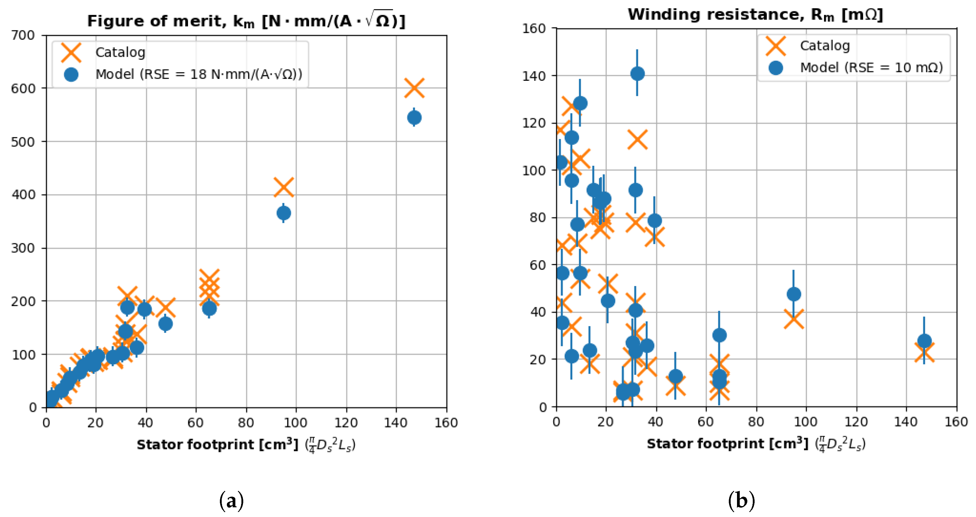
Figure 14a plots the predicted and catalog values for the figure of merit ( k m ). The x axis is the stator footprint. The y axis is the figure of merit. The predicted k m values are a function of Equation (19), with an RSE of 18 units. Again, the model accurately predicts k m for motors with a stator footprint up to 80 cm 3 .
Using the predicted k m values and the catalog torque constants ( k t ), we solved Equation (3) for the winding resistances ( R m ) of the motors. We could not predict the catalog motors’ torque constants because the application voltage and speed drive the ideal k t value. In such cases, we recommend an ideal sizing ( k t , i d ) with a 30% buffer ( b m r g = 0.3 ) between back-EMF ( V e d ) at the design speed ( ω d ) and the DC voltage ( V D C ), as expressed in Equation (23).
V e d = ( 1 b m r g ) V D C k t , i d ω d = ( 1 b m r g ) V D C k t , i d = ( 1 b m r g ) V D C ω d
Figure 14b plots the predicted and catalog resistance values. The x axis is the stator footprint, and the y axis is the winding resistance ( R m ). The model predicted resistance with a residual standard error of 10 m Ω . The resistance prediction for the largest motor ( U S F P = 150 cm 3 ) is within the average error bounds, even though the mass and volume predictions are not as accurate for this case. We restricted the resistance model to motors of less than 800 g (80 cm 3  stator footprint) for consistency with the mass model.

5. Full Sizing Algorithm

We integrated the sizing models validated in the preceding section with the efficiency and thermal models we developed and validated in previous papers. We evaluated the full algorithm in the following scenarios:
Case 1.
Experimental validation: We compared the algorithm’s initial size, efficiency, and temperature predictions against experimental data for two different-sized motors under similar loads.
Case 2.
Literature comparison: We compared the algorithm’s iterative predictions to literature models and experimental data.
Case 3.
Broader exploration: We coupled the motor algorithm with a reduced-order battery sizing model and examined the results from a mission-level perspective.

5.1. Experimental Validation

Given shear stress and the ambient conditions, how accurately does the algorithm predict mass, efficiency, and temperature? We fed experimental loads and environmental data for two motors into the algorithm. One motor was larger than the other and operated under a lower shear stress. We compared the algorithm’s initial (non-iterative) mass, efficiency, and temperature predictions with experimental measurements for each motor.
Table 3 lists salient data for the two experimental motors. Reference [19] contains performance data for four different-sized motors under various loads and ambient conditions. We found two data points for which two motors of different sizes operated under the most similar applied loads and ambient conditions. Motor 2’s shear stress is 158% greater than motor 1’s, despite less than 20% differences in the applied torque and freestream velocity. We applied the exact loads and ambient conditions of each data point (motor) to the algorithm and compared its initial predictions with experimental measurements. The mean values are relevant to the next scenario.
First, the algorithm sizes a notional stator footprint from the given torque and shear stress ( U S F P  via Equation (4)). Then, the algorithm estimates the total mass (m via Equation (14)) and outer dimensions ( D o , L o , and U o u t via Equations (16), (17), and (13), respectively). The algorithm uses some of these size predictions to predict the electric constants ( k m , k t , and R m via Equations (19), (23) and (3), respectively).
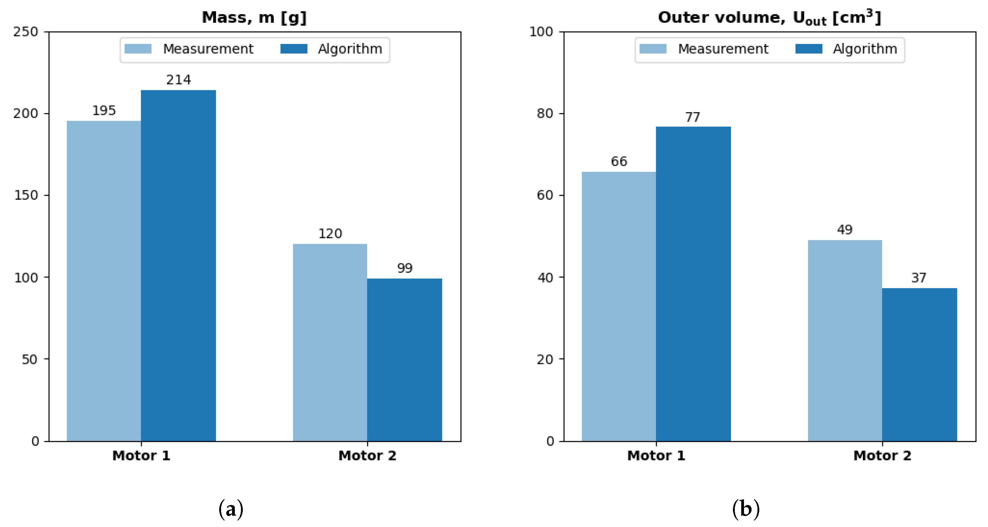
Figure 15a plots the algorithm’s mass prediction and the measured mass for both motor cases. The predicted mass of motor 2 is smaller than that of motor 1 mass, which matches the experimental trend, where mass decreases as shear stress increases. For both motors, the predicted mass is within 20% of the experimental mass, which is acceptable accuracy for a vehicle conceptual design tool.
Figure 15b plots the algorithm’s outer volume predictions alongside measurements. The algorithm, again, captures the experimental trend wherein volume decreases as shear stress increases. The outer-volume predictions for both motors are within 25% of the experimental volume. The volume prediction has poorer accuracy than mass predictions because of error propagation from the outer-diameter ( D o ) and outer-length ( L o ) predictions. Nevertheless, the volume predictions can still reveal valuable trends in the early design stages.
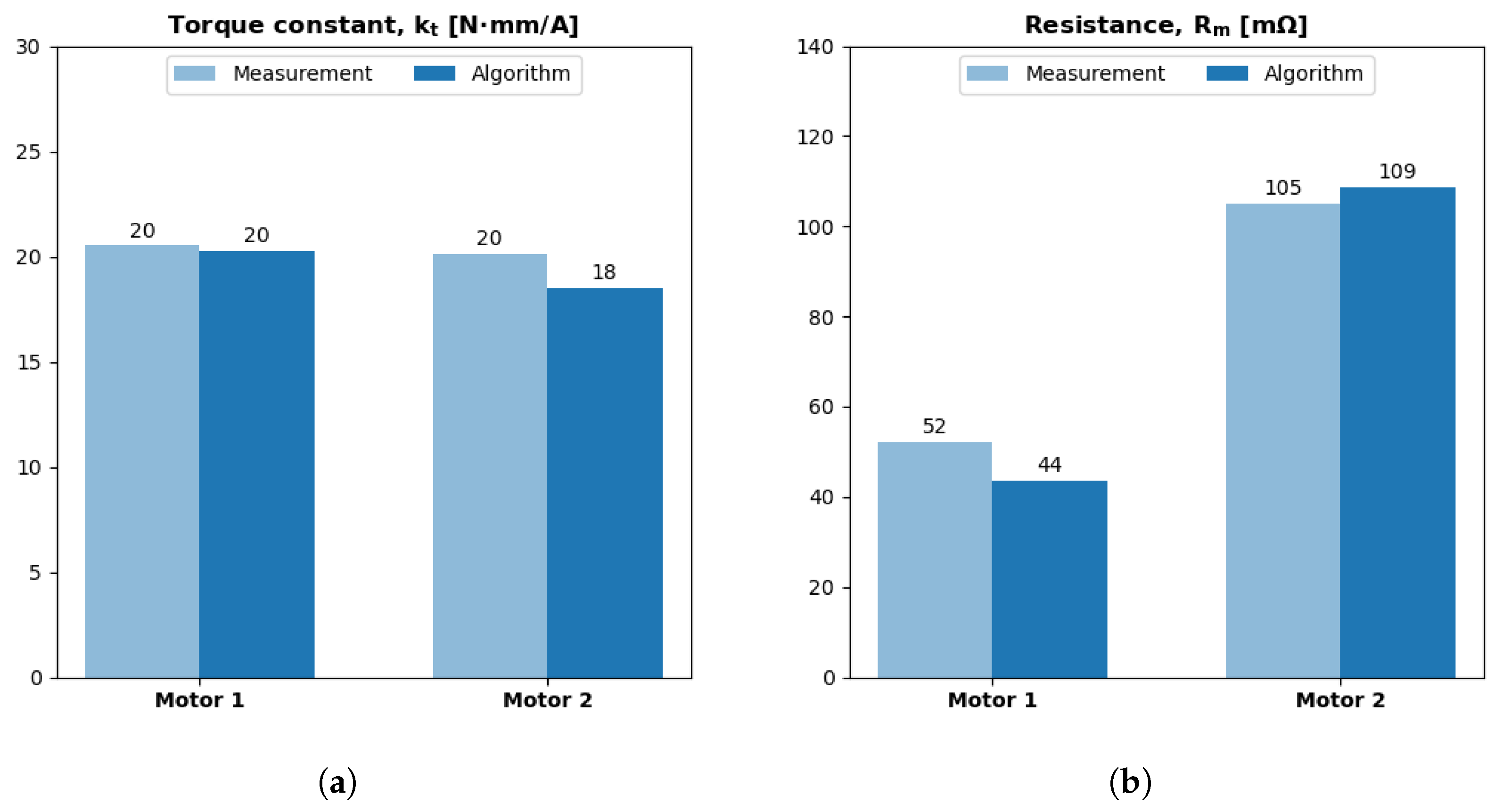
Figure 16a,b plot the algorithm’s predictions for torque constant ( k t ) and winding resistance ( R m ), respectively. The k t prediction error is <10% for both cases, which suggests our 30% margin between back-EMF and the DC voltage in Equation (23) is reasonable. The algorithm underpredicts R m by 16% for motor 1 and overpredicts resistance by only 4% for motor 2. Such accuracy is remarkable, since the resistance prediction inherits errors from upstream k t , U S F P , and D s predictions.
Next, the efficiency model predicts steady-state efficiency ( η , Equation (24)) as a function of the output power ( P o u t ) and total losses ( P l ) using the previously predicted electrical constants ( k t , R m ). The output power is a function of the applied torque and rotational speed ( P o u t = M ω ). The total losses ( P l , Equation (25)) include joule losses ( I 2 R m ) that grow with torque ( I M ) and iron losses ( k t ω I 0 ) that grow with rotational speed and no-load current ( I 0 ). A 10% penalty based on the output power approximates higher-order iron losses. A scaling factor based on the throttle setting (d) approximates harmonic losses associated with modulating voltage. In reference [23], we developed and validated this model with novel powertrain flight data from an instrumented quadcopter.
η = P o u t P i n = P o u t P o u t + P l
P l = 0.1 P o u t + ( I 2 R m + k t ω I 0 ) / d
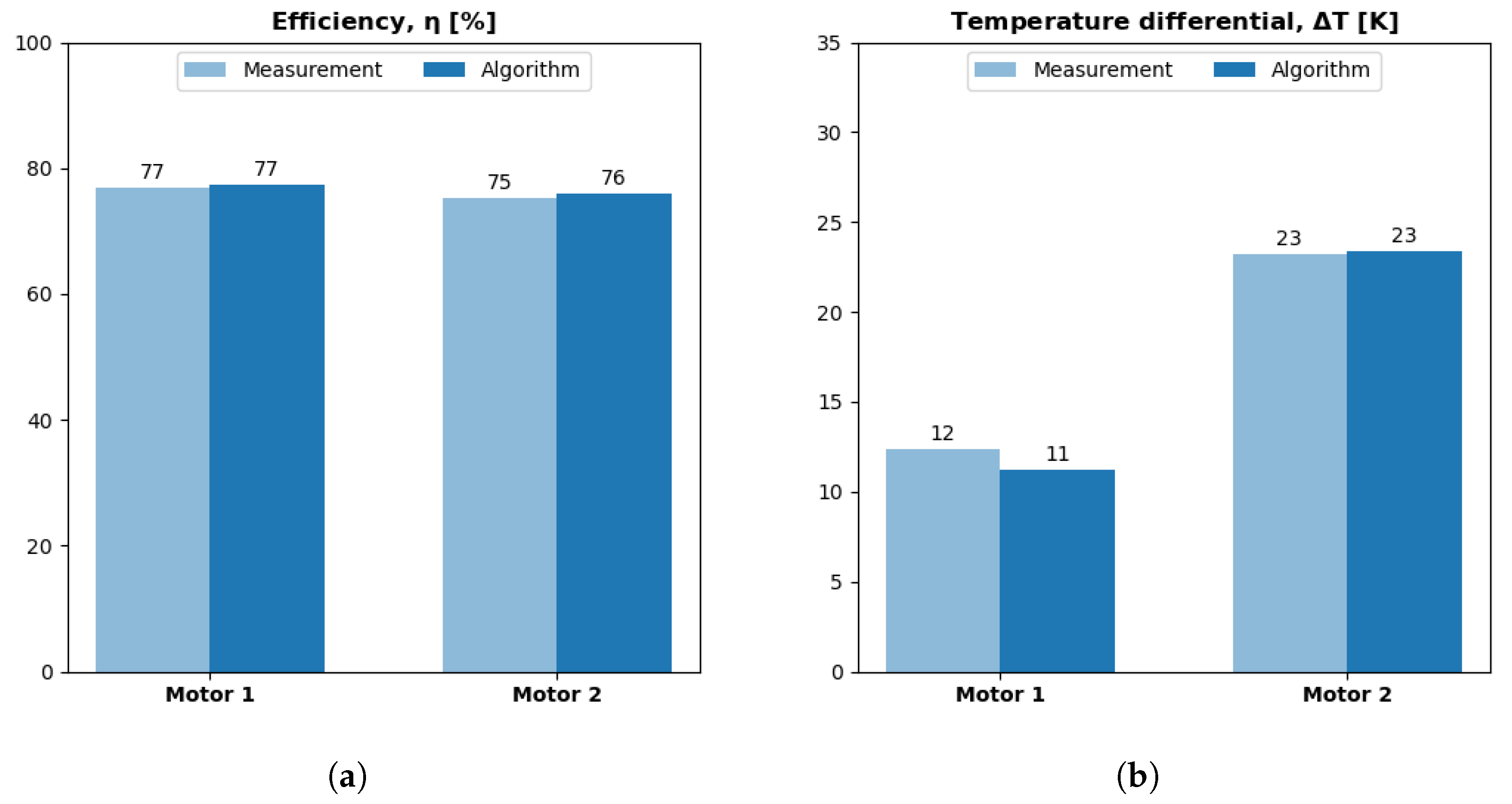
Figure 17a plots the algorithm’s efficiency predictions alongside experimental predictions. The algorithm predicts efficiency with less than 5% error for both motors. The algorithm achieves such accuracy despite upstream errors in the k t and R m predictions, highlighting the efficiency model’s robustness.
The thermal models (Equations (26)–(28)) use the efficiency model’s predicted losses and the sizing models’ predicted dimensions to calculate the motor’s thermal response. First, Equation (26) predicts the Nusselt number ( N u ), a non-dimensional measure of convective heat transfer. The prediction of the Nusselt number is a function of the outer aspect ratio ( A R o = D o / L o ), freestream Reynolds number ( R e i n f = u D o / ν ), and rotational Reynolds number ( R e ω = π 4 D o 2 / ν ). The Reynolds numbers use a constant dynamic viscosity ( ν 15 × 10 6 m 2 /s). Equation (27) calculates the dimensional heat transfer coefficient (h) as a function of the Nusselt number ( N u ), freestream thermal conductivity ( k 26 mW/(m·K)), and the motor’s predicted outer diameter ( D o ). Equation (28) predicts the motor’s freestream temperature differential ( Δ T = T m T ) as a function of the losses ( P l ), heat transfer coefficient (h), and the lateral surface area ( A l a t = π D o L o ). In reference [19], we developed and validated these thermal models with novel wind-tunnel thermal testing of different motors.
N u = 0.01 A R o 1.56 R e 0.39 R e ω 0.66
h = N u k a i r / D o
Δ T = P l / ( h A l a t )
Figure 17b plots the algorithm’s temperature differential predictions alongside experimental measurements. The results show the algorithm accurately captures the coupling between size, efficiency, and temperature; in both cases, the predictions are within 10% of experimental values. The algorithm achieves such accuracy despite upstream error propagation from the sizing and efficiency models and errors within each sizing, efficiency, and thermal sub-routine.

5.2. Literature Comparison

Given the applied load, ambient conditions, and initial shear stress, how do the algorithm’s iterative predictions compare to those of literature models? We fed the algorithm a constant load and freestream conditions and allowed it to iterate until the notional motor overheated. We compared the iterative results to literature model predictions based on the same inputs. We also compared the algorithm’s results to experimental data from similar but not matching loads and conditions.
The mean values listed in Table 3 are the inputs to our algorithm and the literature models. The algorithm began with a conservative shear stress value ( τ 0 < 1 kPa) before incrementing shear stress in each subsequent iteration ( τ i + 1 τ i + 500 Pa). The algorithm stopped when it predicted the motor temperature would meet or exceed 100 °C.
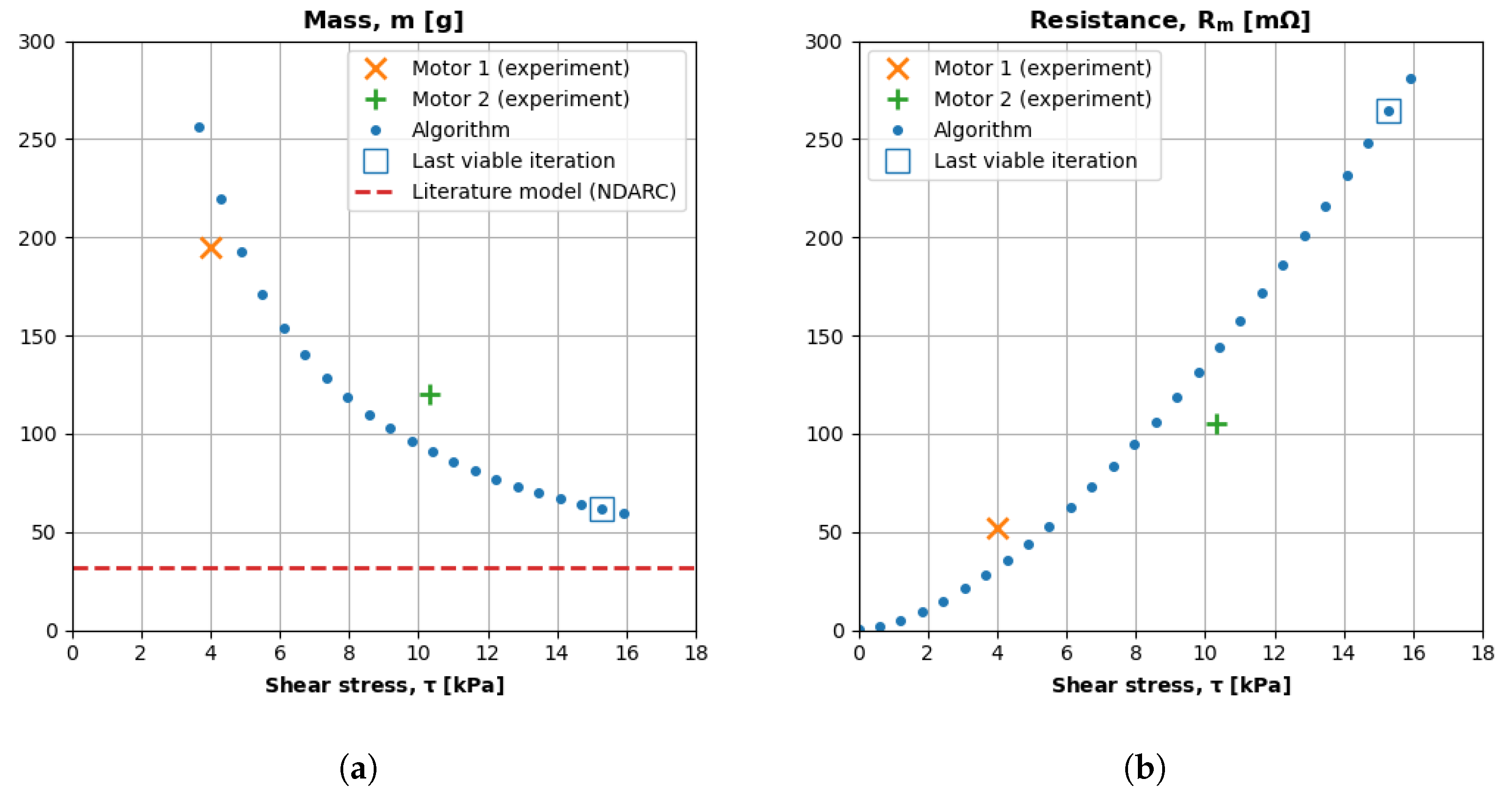
Figure 18a plots the algorithm’s mass predictions. The x axis is the shear stress, and the y axis is the mass. A box highlights the algorithm’s last viable result that does not exceed temperature limits. The figure also plots a mass prediction of a specific torque regression used in two literature models [1,2] and the masses of experimental motors 1 and 2.
The results presented in Figure 18a illustrate that the proposed algorithm can deliver more realistic weight-saving results than literature models. The algorithm nearly quadrupled the notional motor’s specific torque between the first and last viable iterations. The mass estimate shrank from more than 240 g to nearly 60 g at constant torque. The algorithm’s optimal mass (61 g) is 93% greater than the literature estimate (31 g); however, the literature model does not account for thermal effects and does not likely overheat. The algorithm’s mass is slightly larger than motor 1’s mass, at τ = 4 kPa, because motor 1’s applied torque is somewhat larger than the algorithm’s applied torque. Conversely, the predicted mass is slightly smaller than that of motor 2, at τ = 10 kPa, because motor 2’s applied torque is marginally smaller than the algorithm’s applied torque.
Figure 18b plots the algorithm’s iterative winding resistance predictions. The x axis is the shear stress, and the y axis is the winding resistance. The figure also plots the winding resistance for motors 1 and 2. A box highlights the algorithm’s last viable result that does not exceed temperature limits.
The results presented in Figure 18b show how the algorithm captures the experimental trend of increasing resistance, which the literature ignores. A smaller, higher-shear-stress motor (motor 2) has a lower copper volume and, thus, a lower figure of merit ( k m ) than a larger, lower-shear-stress motor (motor 1). A lower k m yields a higher R m at a constant k t . The predicted k t does not change because the operating speed and voltage are constant. Literature models cannot predict any electrical constants.
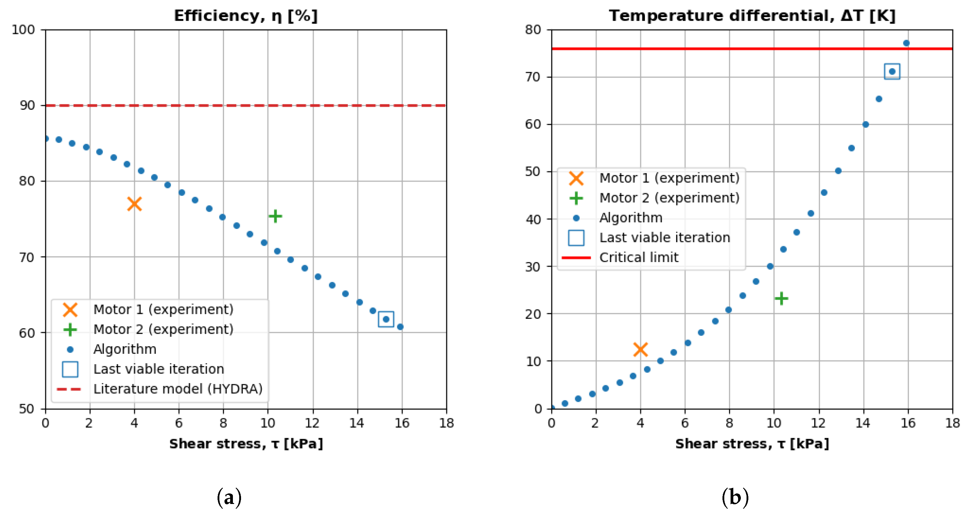
Figure 19a plots the algorithm’s iterative efficiency predictions. The x axis is the shear stress, and the y axis is the efficiency. The figure also plots the experimental efficiency and shear stress for motors 1 and 2, as well as the popular 90% efficiency assumption used in ref. [3]. A box highlights the algorithm’s last viable result that does not result in overheating.
The results presented in Figure 19a show how the algorithm captures a tradeoff of reduced mass that the literature models ignore, namely decreasing efficiency. The first algorithm iteration has an efficiency of about 85%; however, the final motor iteration has an efficiency of about 60%. As a motor shrinks, the resistance increases (Figure 18b), so it generates more waste heat for the same output power (Equation (25)). Even with a dynamic efficiency model, literature sizing approaches cannot capture this trend because they do not model the change in winding resistance with size.
Figure 19b plots the algorithm’s iterative temperature predictions. The x axis is the shear stress, and the y axis is the temperature differential between the motor and ambient environment ( Δ T = T m T ). The figure also plots the experimental temperature differential and shear stress for motors 1 and 2, as well as the limit temperature differential. A box highlights the algorithm’s last viable result that does not result in overheating.
The results presented in Figure 19b illustrate how the algorithm captures the experimental trend of increasing temperature, which the literature ignores. A smaller motor (motor 2) suffers from more heat transfer penalties than a larger motor (motor 1). First, a smaller motor has a smaller lateral surface area to dissipate heat. Second, a smaller motor has a shorter characteristic length; therefore, its corresponding Reynolds and Nusselt numbers are also smaller, reducing its heat transfer coefficient. Third, a smaller motor operates less efficiently and generates higher losses. Literature approaches do not capture this coupling because they ignore thermal effects and assume a constant efficiency.

5.3. System-Level Integration

How does more nuanced motor sizing improve higher-level vehicle design? We combined the motor algorithm with a battery sizing model. The battery model predicted the extra battery mass required to compensate for the decreasing efficiency of an ever-smaller motor. We examined results for different mission lengths and held the motor power requirement constant for simplicity.
Equation (29) computes the change in motor mass ( Δ m m o t ). Equation (30) predicts the energy ( Δ E l o s t ) that the motor wastes as a function of the motor’s power losses and the specified mission duration ( t m i s ). Equation (31) then estimates the extra battery mass ( Δ m b a t t ) that corresponds to the additional energy demand. We assumed a battery density ( e b a t t ) of 170 Wh/kg (612 kJ/kg). All variable changes are relative to the respective values from the first iteration. Equation (32) computes the net change in mass ( Δ m n e t ) from the combined changes in motor and battery weight.
Δ m m o t i = m m o t i m m o t 0
Δ E l o s t i = ( P l i P l 0 ) t m i s
Δ m b a t t i = Δ E l o s t i / e b a t t
Δ m n e t i = Δ m m o t i + Δ m b a t t i
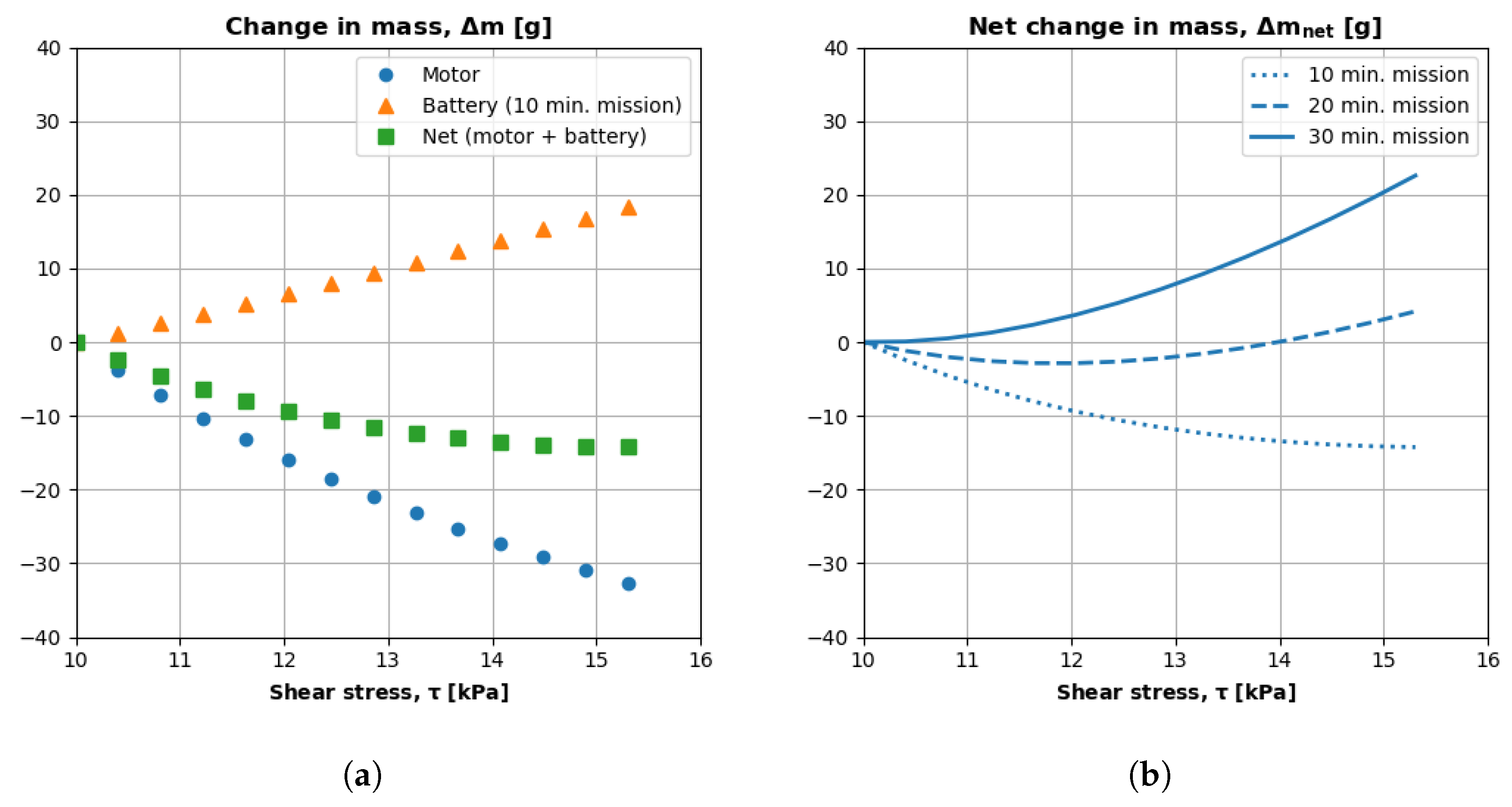
Figure 20a plots the predicted mass changes for a 10-min mission. The x axis is the shear stress, and the y axis is the change in mass relative to the initial iteration. The blue dots are the changes in motor mass, and the orange triangles are the changes in battery mass. The green squares are the sum of motor and battery mass changes.
The results presented in Figure 20a show that a decreasing motor mass can have diminishing returns. At τ 15 kPa, the net mass experiences an inflection point. The extra battery mass required to compensate for the motor’s decreasing efficiency negates the mass savings accrued by shrinking the motor.
The diminishing returns of reducing motor mass are more apparent in Figure 20b. This figure plots the net change in mass (y axis) versus motor shear stress (x axis) for missions of increasing duration. As the mission length increases, the net change in mass increases because the increasingly smaller and less efficient motors consume more power throughout the mission. Therefore, a vehicle must carry extra battery mass to ensure the motor can operate for the mission’s duration. Literature models cannot deliver such broad insights because they assume constant efficiency and do not capture the additional harmful couplings between size (mass), efficiency, and cooling.

6. Discussion

We highlight key results and contributions from the analytical algorithm and the experimental teardown. We also acknowledge this study’s limitations and outline steps to address them in future work.

6.1. Analysis

The algorithm is greater than the sum of its constituent sizing, efficiency, and thermal models. Teardown ((Figure 9)) revealed that motors exhibit a constant 10.3 g/ cm 3 density defined as ρ = m / U S F P . This suggests that a specific iterative torque approach could accurately size mass if each iteration also predicts temperature. Specific torque ( M / m ) has the same units as τ / ρ . Our teardown shows ρ is constant, so iterating over M / m with thermal feedback (an improved literature approach) is no different than iterating over τ with thermal feedback (our approach). However, cooling is a function of the environment, geometry, and efficiency, which is a function of a motor’s electrical constants. Literature models assume a constant efficiency and cannot predict a motor’s dimensions or its internal electrical constants [1,3,14]. Our algorithm has models that capture each size, efficiency, and thermal facet, and the different models intelligently share their predictions to deliver more nuanced and realistic results.
Motor teardown contributes parametric experimental data to the scientific literature. Other research efforts detail the design of singular motors, such as Oak Ridge National Laboratory’s exhaustive teardown of the Toyota Prius’ motor generator [21]. However, these data are not practical for small UAS conceptual designers who are more interested in general trends for various sizes and geometries. Our teardown addresses this knowledge gap despite only examining motors with a stator aspect ratio greater than 1.0.
Researchers and practitioners can use the teardown data to develop other sizing models or even parameterize other models. For example, transient motor thermal models need the constituent component masses to predict temperature rise [8]. Users can estimate the masses of a notional motor’s stator, rotor, bearing, etc., with the presented mass fraction trends. Motor designers can even use the teardown data to validate new designs, since new commercial motors are typically incremental variations of existing designs [24]. For example, teardown motors 5 and 7 in Table 1, which are from the same manufacturer, are identical except for their length.
The sizing algorithm contributes analytical models to the scientific literature. Existing small UAS design codes only provide a single-size estimate that ignores thermal effects and assumes an ideal and constant motor efficiency. Moreover, the existing approaches rely on inter-domain regressions (electromagnetic torque/mechanical mass), whose underlying data were not collected under the same thermal conditions [1,2]. Our algorithm couples sizing, efficiency, and thermal models to deliver more nuanced results. For example, the algorithm captures how decreasing the motor size under constant load and freestream conditions reduces efficiency and increases operating temperature. The algorithm’s empirical regressions are strictly between mechanical parameters, such as mass vs. volume (Equation (14)) or stator vs. outer diameter (Equation (16)); therefore, the regressions are unaffected by different thermal conditions. In finding the lightest motor, the model also offers intermediary options that are heavier but operate more efficiently and at a lower steady-state temperatures.
Researchers and practitioners can implement our approach in existing vehicle design codes to enable system-level optimization. As mentioned, a smaller motor is less efficient and requires more input power to deliver the same output power. For long-duration missions, the extra battery weight needed to compensate for lower motor efficiency may negate the weight savings resulting from shrinking the motor. Our algorithm can help identify such inflection points by capturing a motor’s mass, efficiency, and thermal coupling.

6.2. Future Work

There seems to be a linear relationship between shear stress and motor efficiency. The algorithm predicts a nearly linear decrease in efficiency as shear stress increases (Figure 19a) for a constant output torque and rotational speed (and thus, constant output power). Increasing shear stress reduces volume, and reducing volume decreases the figure of merit ( k m ), which reduces a motor’s ability to convert current into torque rather than waste heat. Therefore, the observed trend principally agrees with the theory. In the future, researchers can attempt to derive an analytical expression to explain this phenomenon.
The presented sizing models cannot predict no-load current ( I 0 ), which is a specification that efficiency models use to predict losses at zero applied torque [4,5,23]. Unfortunately, I 0 is a poor metric for any regression. No-load losses grow as a polynomial function of speed [30], yet datasheets publish I 0 as a scalar value at an unspecified speed. Researchers have an opportunity to address the literature’s lack of suitable no-load loss data and to develop a no-load sizing model. We suggest (1) measuring the no-load mechanical power curve for a variety of motors; (2) fitting a third-order polynomial for each curve; and (3) regressing the polynomial coefficients against key motor specifications such as outer diameter, torque constant, and rotor inertia. The resulting model would predict the no-load power curve coefficients for an arbitrarily sized motor, which efficiency models could use to predict no-load losses at any speed more accurately. We did not have the time and resources to conduct this additional track of experimental and modeling work.
Researchers can tune and validate sizing models to larger air-cooled, radial-flux brushless motors. For example, the algorithm’s sizing accuracy suffers beyond 800 g (Figure 12) because the underlying teardown regression spans 25–600 g motors (Table 1). We optimized our teardown domain to span the widest array of small UAS motors attainable with our budget. A wider regression domain would naturally improve the algorithm’s scope and accuracy. Addressing this shortcoming requires additional destructive teardowns to expand the envelope of the sizing expressions and more thermal testing to inform new regressions for larger motors, particularly in static hover cases where a motor would not experience freestream airflow.
Researchers can also extend the sizing algorithm to other motor topologies like axial-flux motors. These motors often rely on liquid cooling with built-in heat exchangers; therefore, both the sizing and thermal models would require extensive re-development and testing. We specifically targeted conventional outrunner radial-flux motors because they are the most common motors for small UAS. Newer axial-flux motors are found in larger and more expensive manned applications [31], since axial-flux motors offer more specific torque [11,32].
Researchers could also extend the broader algorithm to components like the inverter and battery. In reference [23], we developed efficiency models for the controller and battery. Canonical flat-plate heat transfer models can be used for these components, since they are rectangular prisms that experience freestream convection over their faces. Researchers must find equivalent expressions for the internal sizing models depicted in Figure 4.

7. Conclusions

We developed motor sizing models that integrate with developed efficiency and thermal models in a broader sizing algorithm. The sizing models can predict the mass, dimensions, and electrical constants of outrunner radial-flux brushless DC motors up to 800 g. A teardown of seven motors that varied in mass (24–600 g) and geometry (stator aspect ratio 1.4–9.0) informed the sizing models. Validated against an independent catalog of 30 motors, the sizing models predicted mass and resistance within 10% and 20% of catalog specifications, respectively. Validated against experimental data, the algorithm predicted mass, efficiency, and temperature within 20%, 5%, and 10% accuracy, respectively. The algorithm also captured tradeoffs between size, efficiency, and thermal response that literature models ignore.

Author Contributions

Conceptualization, F.S.; Formal analysis, F.S.; Funding acquisition, M.B.; Investigation, F.S.; Methodology, F.S.; Project administration, M.B.; Supervision, M.B.; Visualization, F.S.; Writing—original draft, F.S.; Writing—review and editing, M.B. All authors have read and agreed to the published version of the manuscript.

Funding

This research was sponsored by the Army Research Laboratory and was accomplished under Cooperative Agreement Number W911NF2020208. The views and conclusions contained in this document are those of the authors and should not be interpreted as representing the official policies, either expressed or implied, of the Army Research Laboratory or the U.S. Government. The U.S. Government is authorized to reproduce and distribute reprints for Government purposes notwithstanding any copyright notation herein.

Data Availability Statement

The original data presented in the study are openly available in Figshare, https://doi.org/10.6084/m9.figshare.26107465, accessed on 26 June 2024.

Acknowledgments

We thank Charlie Gordon for helping with the teardowns.

Conflicts of Interest

The authors declare no conflicts of interest.

Nomenclature

AArea [ m 2 ]
A R s Stator aspect ratio [-]
BMotor magnetic loading [T]
b m r g Back-EMF margin [-]
DDiameter [m]
dThrottle setting (duty-ratio) [-]
EEnergy [J]
eSpecific energy [J/kg]
hConvective heat transfer coefficient [W/( m 2 · K)]
ICurrent [A]
k a i r Air thermal conductivity [W/(m·K)]
k t Motor torque constant [N/(m·A)]
LLength [m]
MTorque [N·m]
mMass [m]
N u Nusselt number [-]
PPower [W]
R e Reynolds number [-]
R m Motor winding resistance [ Ω ]
TTemperature [K]
tTime [s]
UVolume [ m 3 ]
uVelocity [m/s]
V D C DC voltage [V]
wMass (weight) fraction [-]
ζ Resistivity per unit length [ Ω · m]
η Efficiency [-]
ν Dynamic viscosity [ m 2 /s]
ρ Density [kg/ m 3 ]
τ Electromagnetic shear stress [Pa]
ω Rotational speed [rad/s]

References

  1. Johnson, W. NDARC-NASA Design and Analysis of Rotorcraft. In Proceedings of the American Helicopter Society Aeromechanics Specialists’ Conference, San Francisco, CA, USA, 20–22 January 2010; Available online: https://ntrs.nasa.gov/citations/20110002948 (accessed on 28 April 2024).
  2. Vegh, J.M.; Botero, E.; Clark, M.; Smart, J.; Alonso, J.J. Current capabilities and challenges of NDARC and SUAVE for eVTOL aircraft design and analysis. In Proceedings of the 2019 AIAA/IEEE Electric Aircraft Technologies Symposium (EATS), Indianapolis, IN, USA, 19–22 August 2019; IEEE: Piscataway, NJ, USA, 2019; pp. 1–19. [Google Scholar] [CrossRef]
  3. Sridharan, A.; Govindarajan, B.; Chopra, I. A scalability study of the multirotor biplane tailsitter using conceptual sizing. J. Am. Helicopter Soc. 2020, 65, 1–18. [Google Scholar] [CrossRef]
  4. Thurlbeck, A.P.; Cao, Y. Analysis and Modeling of UAV Power System Architectures. In Proceedings of the 2019 IEEE Transportation Electrification Conference and Expo (ITEC), Detroit, MI, USA, 19–21 June 2019; pp. 1–8. [Google Scholar] [CrossRef]
  5. Gong, A.; MacNeill, R.; Verstraete, D. Performance Testing and Modeling of a Brushless DC Motor, Electronic Speed Controller and Propeller for a Small UAV Application. In Proceedings of the 2018 Joint Propulsion Conference, Cincinnati, OH, USA, 9–11 July 2018. [Google Scholar] [CrossRef]
  6. Ma, Y.; Zhang, W.; Zhang, Y.; Ma, Y.; Bai, Z. Preliminary Design and Experimental Investigation of a Distributed Electric Propulsion Aircraft. In Proceedings of the 32nd Congress of the International Council of the Aeronautical Sciences (ICAS), Shanghai, China, 6–10 September 2021; pp. 6–10. [Google Scholar]
  7. Perry, A.T.; Ansell, P.J.; Kerho, M.F. Aero-propulsive and propulsor cross-coupling effects on a distributed propulsion system. J. Aircr. 2018, 55, 2414–2426. [Google Scholar] [CrossRef]
  8. Liang, D.; Zhu, Z.; Feng, J.; Guo, S.; Li, Y.; Wu, J.; Zhao, A. Influence of critical parameters in lumped-parameter thermal models for electrical machines. In Proceedings of the 2019 22nd International Conference on Electrical Machines and Systems (ICEMS), Harbin, China, 11–14 August 2019; IEEE: Piscataway, NJ, USA, 2019; pp. 1–6. [Google Scholar] [CrossRef]
  9. Tong, W. Mechanical Design and Manufacturing of Electric Motors; CRC Press: Boca Raton, FL, USA, 2022. [Google Scholar] [CrossRef]
  10. Mohan, N. Electric Machines and Drives, 1st ed.; Wiley: Hoboken, NJ, USA, 2012; Available online: https://books.google.com.hk/books?id=G-xHDwAAQBAJ&printsec=copyright&redir_esc=y#v=onepage&q&f=false (accessed on 1 June 2024).
  11. Hamdi, E.S. Design of Small Electrical Machines; John Wiley & Sons, Inc.: Hoboken, NJ, USA, 1994; Available online: https://dl.acm.org/doi/abs/10.5555/561305 (accessed on 28 April 2024).
  12. Hendershot, J.; Miller, T. Design of Brushless Permanent-Magnet Machines; Oxford Academic: Oxford, UK, 2010. [Google Scholar] [CrossRef]
  13. Kirchgässner, W.; Wallscheid, O.; Böcker, J. Estimating electric motor temperatures with deep residual machine learning. IEEE Trans. Power Electron. 2020, 36, 7480–7488. [Google Scholar] [CrossRef]
  14. Ugwueze, O.; Statheros, T.; Horri, N.; Bromfield, M.A.; Simo, J. An Efficient and Robust Sizing Method for eVTOL Aircraft Configurations in Conceptual Design. Aerospace 2023, 10, 311. [Google Scholar] [CrossRef]
  15. Miyairi, Y.; Perullo, C.; Mavris, D.N. A parametric environment for weight and sizing prediction of motor/generator for hybrid electric propulsion. In Proceedings of the 51st AIAA/SAE/ASEE Joint Propulsion Conference, Orlando, FL, USA, 27–29 July 2015; p. 3887. [Google Scholar] [CrossRef]
  16. Tursini, M.; Villani, M.; Fabri, G.; Di Leonardo, L. A switched-reluctance motor for aerospace application: Design, analysis and results. Electr. Power Syst. Res. 2017, 142, 74–83. [Google Scholar] [CrossRef]
  17. Dussart, G.X.; Lone, M.M.; O’Rourke, C. Size estimation tools for conventional actuator system prototyping in aerospace. In Proceedings of the AIAA Scitech 2019 Forum, San Diego, CA, USA, 7–11 January 2019; p. 1634. [Google Scholar] [CrossRef]
  18. Roussel, J.; Budinger, M.; Ruet, L. Preliminary Sizing of the Electrical Motor and Housing of Electromechanical Actuators Applied on the Primary Flight Control System of Unmanned Helicopters. Aerospace 2022, 9, 473. [Google Scholar] [CrossRef]
  19. Saemi, F.; Whitson, A.; Benedict, M. Heat Transfer Models and Measurements of Brushless DC Motors for Small UASs. Aerospace 2024, 11, 401. [Google Scholar] [CrossRef]
  20. Koegler, L. KDE4215XF-465 Brushless DC Motor; KDE Direct, LLC: Bend, OR, USA, 2024; Available online: https://www.kdedirect.com/blogs/news/18013663-4215xf-465-uas-brushless-motor (accessed on 28 April 2024).
  21. Burress, T.A.; Campbell, S.L.; Coomer, C.; Ayers, C.W.; Wereszczak, A.A.; Cunningham, J.P.; Marlino, L.D.; Seiber, L.E.; Lin, H.T. Evaluation of the 2010 Toyota Prius Hybrid Synergy Drive System; Technical report; Oak Ridge National Lab. (ORNL): Oak Ridge, TN, USA, 2011. [Google Scholar] [CrossRef]
  22. Staunton, R.H.; Burress, T.A.; Marlino, L.D. Evaluation of 2005 Honda Accord Hybrid Electric Drive System; Technical report; Oak Ridge National Lab. (ORNL): Oak Ridge, TN, USA, 2006. [Google Scholar] [CrossRef]
  23. Saemi, F.; Benedict, M. Flight-Validated Electric Powertrain Efficiency Models for Small UASs. Aerospace 2023, 11, 16. [Google Scholar] [CrossRef]
  24. Hanselman, D. Brushless Permanent Magnet Motor Design. The Writers’ Collective. 2003. Available online: https://digitalcommons.library.umaine.edu/fac_monographs/231 (accessed on 24 June 2024).
  25. Bolam, R.C.; Vagapov, Y.; Anuchin, A. Performance Comparison between Copper and Aluminium Windings in a Rim Driven Fan for a Small Unmanned Aircraft Application. In Proceedings of the 2020 XI International Conference on Electrical Power Drive Systems (ICEPDS), St. Petersburg, Russia, 4–7 October 2020; pp. 1–6. [Google Scholar] [CrossRef]
  26. Hughes, A.; Drury, W. Electric Motors and Drives: Fundamentals, Types and Applications; Newnes: Oxford, UK, 2013. [Google Scholar] [CrossRef]
  27. Koegler, L. KDE 10218XF-105 Brushless DC Motor; KDE Direct, LLC: Bend, OR, USA, 2024; Available online: https://www.kdedirect.com/products/kde10218xf-105 (accessed on 24 June 2024).
  28. Koegler, L. KDE 4014XF-380 Brushless DC Motor; KDE Direct, LLC: Bend, OR, USA, 2024; Available online: https://www.kdedirect.com/products/kde4014xf-380 (accessed on 24 June 2024).
  29. Koegler, L. KDE3510XF-475 Brushless DC Motor; KDE Direct, LLC: Bend, OR, USA, 2024; Available online: https://www.kdedirect.com/products/kde3510xf-475 (accessed on 24 June 2024).
  30. Toliyat, H.A.; Kliman, G.B. Handbook of Electric Motors; CRC Press: Boca Raton, FL, USA, 2018. [Google Scholar] [CrossRef]
  31. Coleman, D.; Halder, A.; Saemi, F.; Runco, C.; Denton, H.; Lee, B.; Subramanian, V.; Greenwood, E.; Lakshminaryan, V.; Benedict, M. Development of “Aria” a Compact, Quiet Personal Electric Helicopter. J. Am. Helicopter Soc. 2023, 68, 42011–42024. [Google Scholar] [CrossRef]
  32. Bird, J.Z. A Review of Electric Aircraft Drivetrain Motor Technology. IEEE Trans. Magn. 2022, 58, 1–8. [Google Scholar] [CrossRef]
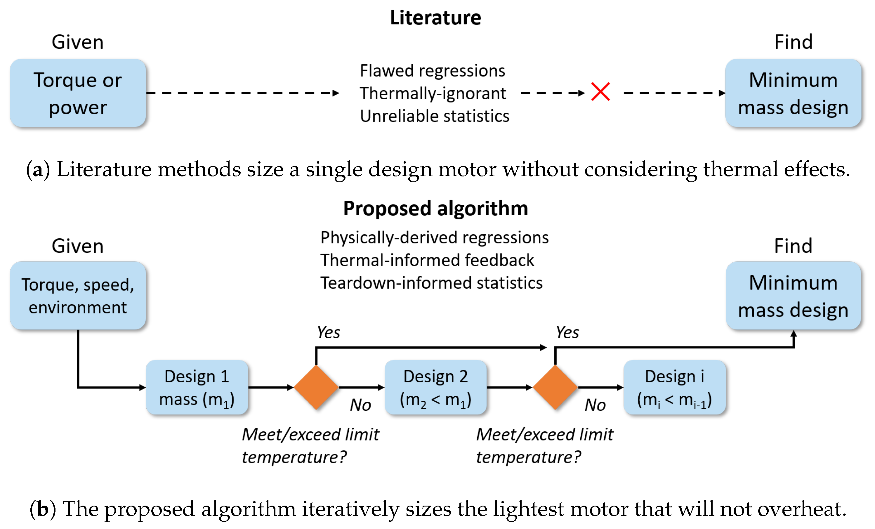
Figure 1. Comparing our approach to literature methods.
Aerospace 11 00649 g001
Figure 2. An outrunner brushless DC motor and its stator and rotor assemblies.
Aerospace 11 00649 g002
Figure 3. The proposed algorithm and its key model blocks.
Aerospace 11 00649 g003
Figure 4. The internal functions of the Sizing models block that is highlighted in Figure 3.
Aerospace 11 00649 g004
Figure 5. Motor teardown process.
Aerospace 11 00649 g005
Figure 6. Key motor components and their dimensions.
Aerospace 11 00649 g006
Figure 7. The seven teardown motors vary in mass and stator aspect ratio.
Aerospace 11 00649 g007
Figure 8. Analysis of the electromagnetically active stator and rotor. (a) The stator and rotor constitute about 70% of a motor’s total mass. (b) The stator and rotor densities are both nearly 6 g/ cm 3 .
Aerospace 11 00649 g008
Figure 9. m / U S F P is surprisingly more consistent than m / U o u t .
Aerospace 11 00649 g009
Figure 10. Analysis of the stator and outer dimensions. (a) The stator drives outer diameter across all aspect ratios. (b) The stator only drives outer length at low aspect ratios.
Aerospace 11 00649 g010
Figure 11. Figure-of-merit trends for the teardown motors.
Aerospace 11 00649 g011
Figure 12. Equation (14) can accurately predict mass up to 800 g. (a) Mass predictions for the entire catalog. (b) Model accuracy improves below 800 g.
Aerospace 11 00649 g012
Figure 13. Model predictions of a motor’s outer dimensions. (a) Predictions of outer diameter. (b) Predictions of outer length.
Aerospace 11 00649 g013
Figure 14. Model predictions of a motor’s electrical constants. (a) Predictions of the figure of merit. (b) Predictions of winding resistance.
Aerospace 11 00649 g014
Figure 15. Algorithm predictions for mass and volume. For each motor case, model error = (algorithm − measurement)/measurement. (a) Model errors are 10% and −17%, respectively. (b) Model errors are 17% and −24%, respectively.
Aerospace 11 00649 g015
Figure 16. Algorithm predictions for electrical constants. For each motor case, model error = (algorithm − measurement)/measurement. (a) Model errors are −5% and −10%, respectively. (b) Model errors are −16% and 4%, respectively.
Aerospace 11 00649 g016
Figure 17. Algorithm predictions for efficiency and freestream temperature differential. For each motor case, model error = (algorithm − measurement)/measurement. (a) Model errors are −9% and 4%, respectively. (b) Model errors are −9% and 4%, respectively.
Aerospace 11 00649 g017
Figure 18. Algorithm mass and resistance predictions. (a) The algorithm reduces mass by a factor of 1 4 between the first and last viable iterations. (b) Resistance increases as size and internal copper volume decrease.
Aerospace 11 00649 g018
Figure 19. Algorithm efficiency and temperature predictions. (a) The popular 90% assumption is unrealistic for small UAS motors. (b) Temperature increases as size decreases.
Aerospace 11 00649 g019
Figure 20. Motor algorithm predictions coupled with a battery sizing model. (a) Reducing motor mass can result in diminishing returns overall. (b) Longer flight times amplify the diminishing returns of reduced motor mass.
Aerospace 11 00649 g020
Table 1. Salient specifications of the teardown motors listed in order of increasing mass.
Motor 1234567
Mass, m[g]244997208379412598
Stator aspect ratio, A R s [-]5.81.82.01.89.01.44.8
Stator inner diameter, D s [mm]10.09.512.712.929.713.929.9
Stator diameter, D s [mm]23.022.028.035.072.041.072.0
Rotor inner diameter, D r i [mm]21.222.929.036.073.041.673.2
Motor outer diameter, D o [mm]27.526.936.043.080.150.081.0
Stator length, L s [mm]4.012.014.020.08.030.015.0
Motor outer length, L o [mm]16.026.031.745.042.564.549.5
Table 2. The mass fractions of each motor’s constituent components.
Motor1234567
Stator0.320.410.390.500.450.500.50
Rotor0.280.310.360.250.160.280.19
Stator support0.120.090.100.040.130.010.04
Rotor support0.120.120.070.100.140.140.15
Bearings0.110.030.050.050.070.020.08
Shaft0.050.030.040.050.060.040.05
Table 3. Salient specifications of two different-sized motors operating under similar conditions.
Motor 1Motor 2Mean
Massm195120158g
Applied torqueM167199183N·mm
Applied rotational speed ω 396547004333 1 / min
Freestream velocity u 9.810.310.1m/s
Freestream temperature T 24.024.024.0°C
Shear stress τ 4.010.37.2kPa
Stator aspect ratio A R s 2.83.53.2
DC voltage V D C 12.013.012.5V
No-load current I 0 0.20.70.5A
Full motor specifications Ref. [20]Ref. [29]
Disclaimer/Publisher’s Note: The statements, opinions and data contained in all publications are solely those of the individual author(s) and contributor(s) and not of MDPI and/or the editor(s). MDPI and/or the editor(s) disclaim responsibility for any injury to people or property resulting from any ideas, methods, instructions or products referred to in the content.