Abstract
Because fixed-wing unmanned aerial vehicles (UAVs) require high-speed taxiing for takeoff and landing, the aircraft’s stability during taxiing is critical. However, despite research on the taxiing stability of fixed-wing UAVs conducted in taxiing motion simulations employing various tire models, the applicability of the models to fixed-wing UAV taxiing simulations remains unclear, as does the rationale behind the parameter settings in the models. Therefore, in our study, we measured the forces acting on the tires of a fixed-wing UAV under various conditions, including tire loads of 1.6–3.6 kg and tire slip angles of 0–40 deg. Based on the results, we modified conventional tire models and assessed their applicability in taxiing simulations. Among our findings, the parameter values of the models significantly differed from those used in crewed aircraft taxiing simulations, and the presence or absence of load parameters in the lateral force tire models significantly affected the dynamics. Furthermore, the aerodynamics acting on the aircraft enhanced the straight-line stability during taxiing, resulting in reduced forces on the tires.
1. Introduction
Following advancements in flight control technology, unmanned aerial vehicles (UAVs) are increasingly used in various fields. Compared to rotary-wing UAVs, including multirotor UAVs, fixed-wing UAVs offer several advantages, including the capability of high-speed flight, greater flight energy efficiency that enables longer flight durations, and the capacity for larger payloads [1]. These characteristics make fixed-wing UAVs especially suitable for applications that require long-range transportation and wide-range ground observation [2,3,4,5].
Because fixed-wing UAVs rely on the lift generated by their wings for takeoff, they require high-speed taxiing on runways during takeoff and landing. Therefore, the stability of fixed-wing UAVs during taxiing is crucial for safe takeoffs and landings. The importance of taxiing stability during takeoff and landing has also been emphasized for aircraft considering that runway incidents account for a significant proportion of all accidents [6,7,8]. Aircraft that lack stability during taxiing may find it difficult to steer in the desired direction using steering maneuvers, thereby leading to potential runway excursions or the failure to reach takeoff speed. Because such events can also occur with fixed-wing UAVs, it is essential to evaluate their stability during taxiing in the design stage in order to ensure their safe and reliable takeoff and landing.
Research on the taxiing stability during the takeoff and landing of aircraft and fixed-wing UAVs is primarily conducted using simulations. In one study, Brott [9] analyzed the lateral stability of tailwheel airplanes during takeoff and landing taxiing using a two-wheel mathematical model in order to evaluate how the mutual positioning of the wheels, the center of gravity, and the vertical tail affected the stability. In another, Khapane [10] simulated aircraft taxiing, proposed an antilock brake system algorithm, and demonstrated the algorithm’s effectiveness in reducing the stopping distance and vibrations of the aircraft. In other work, Rankin et al. [11,12] performed bifurcation analysis as a new method of evaluating the stability of aircraft ground dynamics and observed qualitative changes in the region of stable solutions when thrust levels varied in both heavy and light aircraft. Turbuk and Paglione [13], meanwhile, proposed a five-degrees-of-freedom aircraft motion model for conducting runway speed control with simple velocity control, and Georgieva and Serbezov [14] investigated the effects of aircraft weight and center-of-gravity positioning to reveal that increased front gear loads heightened lateral instability. Moreover, Song et al. [15] evaluated the factors leading to ground loops in fixed-wing UAVs with flying-wing shapes using simulation, which indicated that reducing the front-wheel load could avoid ground loops. In addition, Hou et al. [16] conducted a ground dynamics analysis of three-wheeled UAVs with varying taxiing speeds and steering angles, thereby clarifying the range between overturning and non-overturning conditions. Finally, Yin et al. [17,18] conducted a bifurcation analysis of fixed-wing UAVs to assess the effects of the aircraft speed, steering angle, and rudder on stability and, as a result, elucidated the transition between stable and unstable states and their causes.
As mentioned above, evaluating the taxiing stability during the takeoff and landing of aircraft and fixed-wing UAVs involves constructing motion models in simulations, altering parameters that influence the aircraft’s motion, and assessing the impact of those parameters on the motion. The key parameters affecting aircraft motion include the aircraft’s mass, center of gravity, landing gear arrangement, aerodynamics, and tire forces.
A point of interest in conventional research using simulated taxiing is the application of various models of tire dynamics. Indeed, because the forces acting on the tires are crucial parameters that directly influence the movement of aircraft during taxiing, conducting taxiing simulations for fixed-wing UAVs requires employing an appropriate tire model. However, the applicability of conventional tire models to such simulations remains unclear. Moreover, though studies on aircraft tend to establish parameter values in tire models based on tire data provided by manufacturers [9], the literature on taxiing simulations for fixed-wing UAVs often lacks citations to the sources of parameter values used in their models.
The purpose of our study is to clarify the tire model parameters that have been unclear in conventional fixed-wing UAV taxiing simulations through parameter identification experiments. We also aimed to clarify the impact of the tire model on the taxiing motion by conducting fixed-wing UAV taxiing simulations.
2. Tire Model
2.1. Tire Coordinate System
Figure 1 presents the coordinate system of the tire examined in our study. Because the coordinate system is fixed to the tire itself, when the tire moves at a velocity with a slip angle , forces are generated along the directions defined by the system. The force acting in the direction , called the “longitudinal force”, is denoted as ; the force generated in the tire’s lateral direction , called the “lateral force”, is denoted as ; and the force acting in the vertical direction perpendicular to the ground, called the “vertical reaction force”, is denoted as .
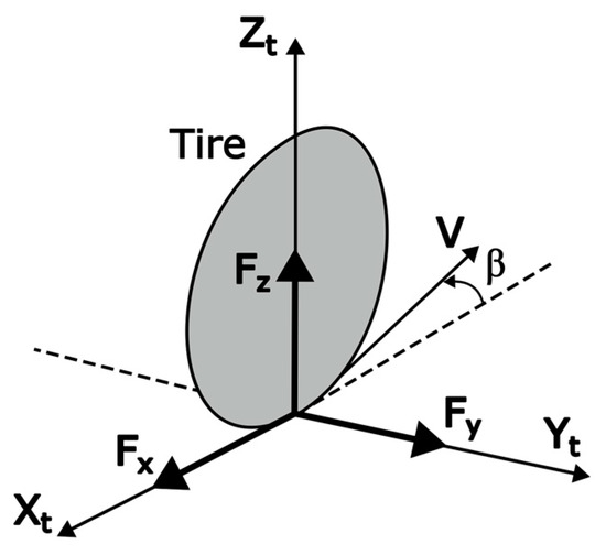
Figure 1.
The definition of the coordinate system and forces acting on the tire.
2.2. Conventional Tire Models
Using the tire-fixed coordinate system shown in Figure 1, we organized the conventional tire models as presented in Table 1, Table 2 and Table 3. The equations in each table were modified from their sources to align with the coordinate system and variable names used in Figure 1.

Table 1.
Longitudinal force tire models.

Table 2.
Lateral force tire models.

Table 3.
Vertical reaction force tire models.
Table 1 presents the conventional tire model equations for the longitudinal force . The tire model for includes a linear model, as shown in Equation (1), and nonlinear models, as indicated in Equations (2)–(4). All models account for variations in in response to changes in the vertical reaction force . The nonlinear tire model in Equation (2) is characterized by a friction coefficient, , which varies as a function. Although Khapane’s [10] article includes graphs of the friction coefficient , it does not provide a specific formula. By comparison, the tire model used by Rankin et al. [11,12], shown in Equations (3) and (4), represents the nonlinearity of with and .
Next, Table 2 presents the conventional tire model equations for the lateral force . Equation (5) describes a linear Coulomb friction model, where changes in response to . Equation (6), by contrast, is a linear model represented by the lateral force coefficient and slip angle , with changing in response to variations in . Equation (7), also a Coulomb friction model, incorporates a friction coefficient, , which varies with the slip angle , the vertical reaction force , and velocity . However, the explicit formula for is not provided in Turbuk and Paglione’s [13] article. Equation (8), known as the “Magic Formula” (MF) tire model proposed by Bakker et al. [19], accurately represents the nonlinear characteristics of in relation to the slip angle by appropriately setting the parameters and . Beyond that, Equation (9) models the nonlinear characteristics of against . Rankin et al. [11,12] designed the equation such that is a quadratic polynomial of , which allows the model to accommodate changes in .
Finally, Table 3 presents the conventional equations for the vertical reaction force . Equation (10) describes a spring–damper model that calculates based on the vertical displacement and velocity displacement of the tire or landing gear. The model is frequently used in the ground dynamics of aircraft and fixed-wing UAVs. Equation (11), by contrast, describes a model that calculates as a polynomial of tire displacement, . In that equation, the coefficients and are set based on tire data.
3. Experiment
Various tire force test machines that are available for automotive tires enable the construction of tire models for motion analysis using individual tire tests. However, no commercially available tire testing devices are specifically designed for use with fixed-wing UAVs. Therefore, we constructed a tire-testing device for UAVs in order to measure tire forces. The forces acting on a tire change based on the load on the tire, slip angle, slip ratio, and velocity [20]. In our study, we focused on the load on the tire, , and the slip angle, as the test parameters that significantly affect tire forces. By varying these parameters, we conducted measurements to understand how changes in them influence the forces exerted on the tire.
3.1. Experimental Method
Figure 2 presents a schematic of the tire force measurement device. The measurement part moves in the forward direction via an electric linear motion system, which causes the tire to roll. The load on the tire is adjusted by placing weights on top of the measurement part. Meanwhile, the slip angle of the tire can be adjusted and fixed at a determined angle using a rotational stage. The Vernier scale of the rotational stage is used to set the angle, tire forces are measured with a load cell located at the top of the tire, and the measurement data are recorded by a data logger. Figure 3 shows the constructed tire force measurement device, while Table 4 lists the specifications of the testing equipment.
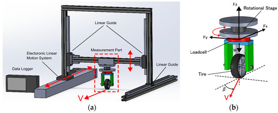
Figure 2.
(a) Schematic of tire force measurement device and (b) measurement part.
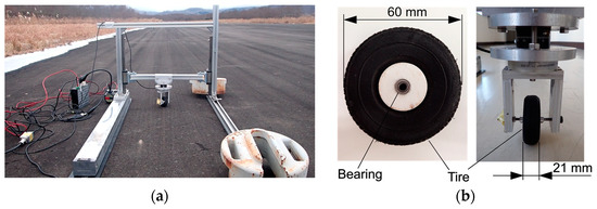
Figure 3.
(a) Constructed tire force measurement device and (b) specimen tire.

Table 4.
Specifications of the experimental equipment and specimen tire.
Table 5 presents the experimental conditions. The load on the tire was set in light of the weight distribution across three tires while assuming the mass of a fixed-wing UAV to be 5–10 kg. The speed of the tire was set at 0.05 m/s to ensure a sufficient number of measurement points within the 1 m length of the electric linear motion system.

Table 5.
Experimental conditions.
3.2. Experimental Results
The results of our measurements appear in Figure 4, Figure 5 and Figure 6. Figure 4 presents the results for the longitudinal force , Figure 5 presents the results for the lateral force , and Figure 6 presents the results for the vertical force . The results plotted in the figures represent the average values obtained from three measurements under the experimental conditions, while the error bars indicate the standard deviation. The forces in each graph follow the coordinate system presented in Figure 1. All measurement results are included in the Supplementary Materials.
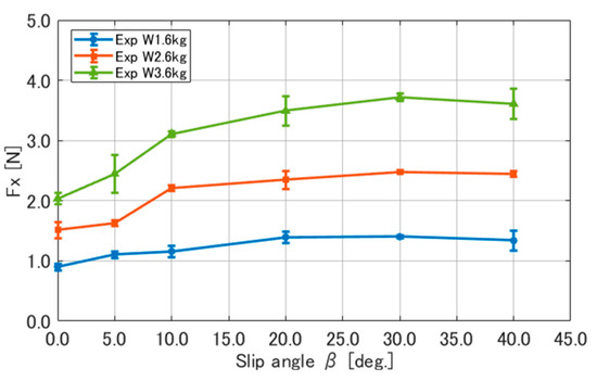
Figure 4.
Results of measuring longitudinal force .
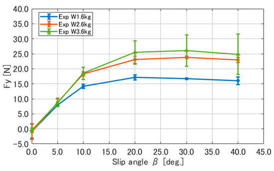
Figure 5.
Results of measuring lateral force .
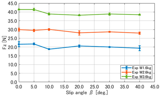
Figure 6.
Results of measuring vertical reaction force .
First, as shown in Figure 4, the longitudinal force increased with an increasing slip angle and load . The rate at which increased also increased nonlinearly with both the slip angle and load .
Next, Figure 5 shows the measurement results of the lateral force , which increased linearly when the slip angle was small, approximately from 0 to 5 deg. When the slip angle exceeded 5 deg., nonlinearity emerged. The change in the lateral force in response to the load change was greater when the load varied from 1.6 to 2.6 kg than when it changed from 2.6 to 3.6 kg. Therefore, also increased nonlinearly in response to the changes in .
Finally, as shown in Figure 6, the vertical force increased by a constant amount with each 1 kg increase in the load , and its magnitude remained nearly constant even when the slip angle varied. This result indicates that a constant reaction force was measured in response to the load. As for the difference between the load and , when the tire was stationary, and matched because the tire was deformed by the load. However, as the tire started to rotate, its undeformed parts made contact with the ground, and the measurement part was pushed upward along the linear guide. Due to slight friction in the guide, the load cell measured as being larger than .
4. Parameter Identification
In our study, we modeled the longitudinal force and lateral force , which significantly affect the taxiing motion of fixed-wing UAVs. The experimental results in Section 3 demonstrate that forces and generated on the tire varied with the tire load and the slip angle . The tire modeling in our study used the actual vertical force on the tire instead of the tire load . Based on the experimental results in Section 3 and the conventional tire models presented in Table 1 and Table 2, we modified the tire models, which included the vertical reaction force and the slip angle as variables.
4.1. Method for Longitudinal Force
Researchers have often employed the Coulomb friction model, shown in Equation (1), to calculate the longitudinal force . The results in Figure 4, by contrast, indicate that while changed linearly in relation to the slip angle , its slope varied with changes in . This dynamic suggests that the friction coefficient changes with variations in . In Table 1, Equation (4) includes only the slip angle as a variable. However, when we tried to model this using Equation (4), the experimental results shown in Figure 4 could not be represented by the equation. For these reasons, we considered two model equations: one in which the friction coefficient in Equation (1) was identified from the experimental results in Figure 4, and the other expressed as a function of and .
4.1.1. Linear Longitudinal Force Model
Equation (1) presents the Coulomb friction model for . The friction coefficient can be determined by dividing the experimental results for by . Equation (1) does not include the slip angle as a variable. Therefore, as shown in Figure 7, the experimental results for each load at a slip angle deg. Were fitted with a linear equation, and the coefficient obtained was designated as . The values of the friction coefficient obtained appear in Figure 7.
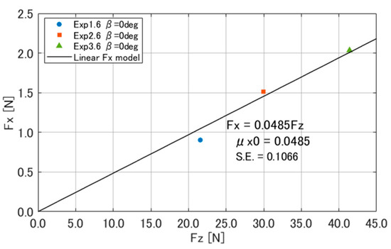
Figure 7.
Slope of in relation to at deg. S.E. = standard error.
4.1.2. Nonlinear Longitudinal Force Model
Next, we constructed a model for considering the slip angle and the vertical reaction force as parameters. As the results in Figure 4 show, varied with the slip angle and , and even at deg., . Based on these characteristics, is expressed by Equation (12), the first term of which represents the longitudinal force when deg. By contrast, the second term represents the increment of due to the slip angle and vertical reaction force . Figure 8 shows a comparison of the obtained from the experimental results and the calculated using Equation (12). The coefficients , , , and in Equation (12) were determined through optimization calculations to minimize the difference between the experimental results and the calculations using the model equation. The fmincon function, a program function in the MATLAB R2022a Optimization Toolbox used to find the minimum value of nonlinear multivariable functions, was used for the optimization calculations.
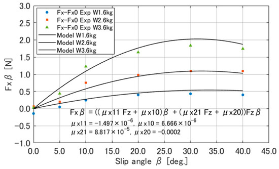
Figure 8.
Results of fitting for each load.
4.2. Method for Lateral Force (
As Table 2 shows, conventional studies have often involved using Equation (6) for the lateral force , which models as changing linearly with the slip angle . However, as Figure 5 shows, becomes nonlinear when the slip angle exceeds the range of 5–10 deg. In response, we employed both the linear model of Equation (6) and the nonlinear models of Equations (8) and (9), each of which has its advantages and disadvantages. The MF, represented by Equation (8), is widely used in the automotive industry and has a proven track record but requires the specification of many parameters for model construction. By contrast, the lateral force model by Rankin et al. represented by Equation (9) requires fewer parameters to be specified; even so, it remains unclear whether it can accurately represent experimental results.
4.2.1. Linear Lateral Force Model
To determine the lateral force coefficient for the linear lateral force model represented by Equation (6), can be calculated by dividing the experimental results for by the slip angle . From the experimental data shown in Figure 5, is taken as the average value of the slopes for each load within the linear range of slip angles, that is, 0–10 deg. The value of obtained appears in Figure 9.
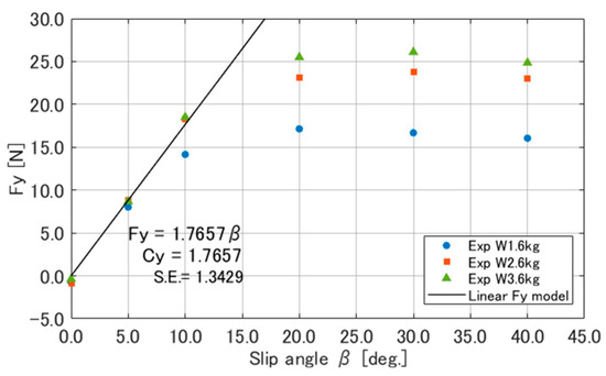
Figure 9.
Comparison of lateral force calculated using Equation (6) and experimental results. S.E. = standard error.
4.2.2. Magic Formula (MF) Tire Model
The MF, represented by Equation (8), was used to analyze the vehicle motion. In the MF, the appropriate settings of the parameters and are crucial. Each parameter plays a unique role in shaping the tire behavior model:
- : stiffness factor (i.e., the product represents the slope at the graph’s origin, indicating the stiffness);
- : shape factor (i.e., determines the overall shape of the graph);
- : peak factor (i.e., specifies the peak value of the graph);
- : curvature factor (i.e., describes the curvature of the graph leading up to the maximum value).
To determine each parameter, we first started with the peak factor . represents the peak value of the lateral force . Figure 5 shows that the peak value of changes with the load. Therefore, in our study, we obtained the peak value of and the corresponding vertical reaction force from Figure 5 and Figure 6, and fitted their relationship to a quadratic equation, as shown in Figure 10. The quadratic equation obtained for is shown in Equation (13).
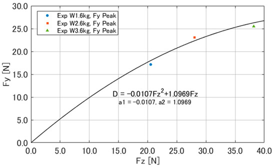
Figure 10.
A quadratic approximation of the peak value of .
The curvature factor can be derived from Equation (14). In Equation (8) of the MF, the lateral force reaches peaks when the argument inside the sine function equals . Therefore, with the sine function’s argument set to and the slip angle at which achieves its maximum value denoted as , can be arranged as shown in Equation (14):
The stiffness coefficient can be determined based on the fact that represents the slope at the origin.
Bakker [19] generalizes by expressing it as a function of , as shown in Equation (15). To determine the coefficients in Equation (15), we used the experimental results for the slip angles from 0 deg. to 10 deg. to obtain the for each load. Beyond that, the average values of for the slip angles from 0 deg. to 10 deg. were used for each load. Figure 11 shows the results of plotting the , obtained using Equation (15), against the experimental results.
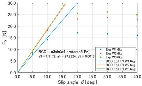
Figure 11.
Fitting of the slope as a function of .
The shape factor can be determined by employing an optimization method. The appropriate parameter was found by minimizing the difference between the experimental results and the values calculated using Equation (8). For optimization, we used the fmincon function in the MATLAB Optimization Toolbox.
Furthermore, the curvature factor was determined using the values of each load according to Equation (14) for the optimized . Bakker [19] represented as a function of , as shown in Equation (16), in order to generalize . Figure 12 shows the fitting results of for each load using Equation (16).
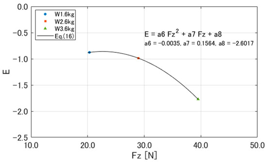
Figure 12.
Quadratic approximation of .
4.2.3. Rankin et al.’s Tire Model
Constructing a lateral force model using Equation (9) requires allowing to vary with the vertical load by making a function of . Rankin et al.’s [11,12] model represents as a quadratic function of , in which is the slip angle at which occurs. can be obtained from the experimental results in Figure 5, and in our study, we expressed as a quadratic function of , similar to the Magic Formula. The quadratic function for can directly utilize Equation (13) to become Equation (17).
4.3. Results of Identification
The parameter values of the tire model obtained in Section 4.2 are summarized below.
4.3.1. Longitudinal Force
Linear Longitudinal Force

Table 6.
Coefficient of linear longitudinal force for .
Nonlinear Longitudinal Force
The coefficients , , , and for Equation (12) obtained from Figure 8 are shown in Table 7. Figure 13 compares the experimental results of with calculated using Equation (12). As shown in Figure 13, the model is capable of representing the changes in in response to the vertical reaction force and the slip angle .

Table 7.
Coefficient of nonlinear longitudinal force model.
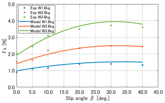
Figure 13.
Comparison of longitudinal force calculated using Equation (12) and experimental results.
4.3.2. Lateral Force Model
Linear Lateral Force Model
Table 8 shows the lateral force coefficient in Equation (6), which differs significantly from that of crewed aircraft. In Georgieva’s aircraft taxiing simulation [14], a lateral force coefficient value of 34.38 [kN/deg.] is used. Furthermore, Brott’s thesis [9] on aircraft taxiing simulation includes lateral force data for various load conditions of aircraft tires from the Goodyear Tire & Rubber Company. Calculating the lateral force coefficient from that data yields values ranging from 0.25 to 0.5 [kN/deg.]. Altogether, that evidence indicates the need to identify the coefficients of any tire lateral force model according to the aircraft and fixed-wing UAV fuselage weight and types of tires.

Table 8.
Coefficient of lateral force model.
Magic Formula (MF) Tire Model
The identified parameters of the MF are shown in Table 9. Figure 14 presents a comparison of the lateral force calculated using the MF and the experimental results for . Based on Figure 14, the MF captured the nonlinear characteristics of the lateral force well and accurately represented the experimental results. Figure 15, using the identified parameters for the MF, is a graph of the lateral force as the vertical reaction force varies from 5 N to 35 N.

Table 9.
Identified parameters of Magic Formula tire model.
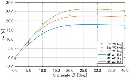
Figure 14.
Comparison of lateral force calculated with Magic Formula tire model and experimental results.
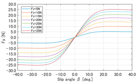
Figure 15.
calculated with the Magic Formula tire model for changes in .
Rankin et al.’s Tire Model
Figure 16 shows a comparison of the lateral force calculated using Equation (9), Equation (17), and the experimental results. Figure 17 presents as the vertical load which varies from 5 N to 35 N. As demonstrated in Figure 16, the model equation from Equation (9) can capture the nonlinear characteristics of the lateral force. Furthermore, Rankin et al.’s tire model has the advantage of being easier to construct than the MF because the MF, shown in Equation (8), requires identifying the parameters and for model construction, whereas Rankin et al.’s tire model, shown in Equation (9), requires only and to be identified.
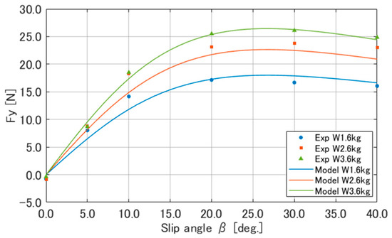
Figure 16.
Comparison of lateral force calculated using Equation (9) and experimental results.
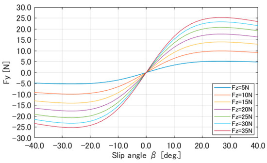
Figure 17.
calculated with Equation (9) for changes in .
5. Simulation
In this section, we describe a taxiing simulation of a fixed-wing UAV performed using the tire models in Section 4. The simulation was aimed at evaluating the differences in motion arising from different tire models and elucidating the impact of tire models on the taxiing dynamics of a UAV.
The fixed-wing UAV airframe model used in the simulation is based on the one-third-scale model of Oowashi, a small winged uncrewed aircraft currently under development at the Muroran Institute of Technology Aerospace System Research Center [21]. The one-third-scale Oowashi serves as a testbed aircraft for realizing the supersonic autonomous flight of fixed-wing UAVs. Figure 18 depicts the one-third-scale Oowashi fuselage. The one-third-scale Oowashi features an elongated shape typical of supersonic aircraft, which is designed to reduce air resistance during high-speed flight. The main wing adopts a cranked arrow wing design.
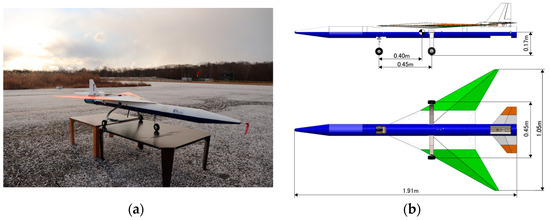
Figure 18.
(a) One-third-scale Oowashi and (b) dimensions of one-third-scale Oowashi.
5.1. Simulation Model
The simulation was conducted using a motion with six degrees of freedom, which treated the airframe as a rigid body. The taxiing motion was calculated using the fourth-order Runge–Kutta method applied to Equations (18) and (19) of the motion equations in the body-fixed coordinate system. In those equations, represents the velocity, represents the external forces, represents the gravity force, represents the moment of inertia, represents angular velocity, and represents the torque. As shown in Equations (20) through (30), the boldface in the equations represents the components of the coordinate system in each axis’s direction as three-dimensional vectors. The tire forces , , and in Equations (23) and (24) are calculated in the tire-fixed coordinate system and transformed into the body-fixed coordinate system using the coordinate transformation matrix and . is the coordinate transformation matrix from the coordinate system fixed to the front tire to the coordinate system fixed to the body, and is the coordinate transformation matrix from the coordinate systems fixed to the left and right tires to the coordinate system fixed to the body. The gravitational force in Equation (25) is calculated in the ground-fixed coordinate system and transformed into the body-fixed coordinate system using the coordinate transformation matrix . The coordinate transformation matrices , and are listed in Appendix A. , , and are the tire torques generated by the tire forces and . The aerodynamic force and the torque are calculated in the body-fixed coordinate system. The terms and in Equation (26) represent the aerodynamic drag and lateral force, respectively. The terms and in Equation (30) represent the rolling moment and yawing moment due to aerodynamics, respectively. Because the one-third-scale Oowashi does not generate lift or a pitching moment at an angle of attack measuring 0 deg., they were not considered in the simulation.
The tire models shown in Table 10 were used in the simulation. The vertical reaction force on the tires was determined using the spring–damper model presented in Equation (10). The spring coefficient and damping coefficient in Equation (10) were set to values that prevented the significant vertical motion of airframes during the simulations.

Table 10.
Tire models in the simulation.
The aerodynamics coefficients , , , and shown in Table 11 were measured by wind tunnel experiments.

Table 11.
Aerodynamic parameters.
Table 12 also lists the specifications of the airframe used, whereas Figure 19 shows the force diagram used in the simulation.

Table 12.
The configuration of the unmanned aerial vehicle.
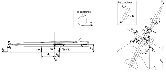
Figure 19.
A force diagram and parameters for a dynamic model of a UAV.
5.2. Simulation Method
In the simulation, two scenarios were conducted: one without considering aerodynamics and the other considering aerodynamics. The former was performed to assess the influence of tire forces on taxiing motion, while the latter was based on the assumption of actual taxiing motion. The simulation cases are shown in Table 13. Case 1.1 compared the linear tire model with the nonlinear tire model. Case 1.2 compared the nonlinear tire model with the MF and Rankin et al.’s tire model. Case 2.1 compared the taxiing motion with and without considering aerodynamics.

Table 13.
Simulation cases.
The evaluation method in the simulation involved assessing the aircraft’s motion and tire forces when the aircraft was subjected to a right turn. The right turn maneuver began by propelling the UAV straight forward with an engine thrust of 45 N from s. Once the UAV speed reached 5.0 m/s, a step input for steering was applied to the front tire to initiate the right turn. The stopping conditions for the simulation were set to occur if either any of the tires lifted off the ground or the slip angle of any tire exceeded 40 deg. The threshold of 40 deg. for the slip angle was determined based on the maximum value of the tire force measurement experiments in Section 2. The simulation time was set to 5 s.
5.3. Results and Discussion
Figure 20, Figure 21, Figure 22, Figure 23, Figure 24 and Figure 25 show the results of the simulation cases presented in Table 13.
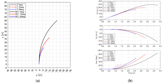
Figure 20.
(a) Trajectories of LT and NT1, and (b) velocities and yaw angles of LT and NT1.
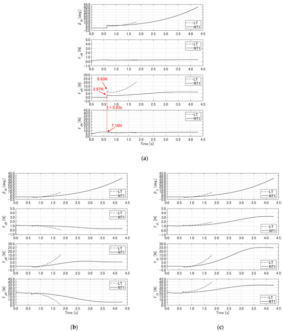
Figure 21.
Comparison of slip angle and tire forces between LT and NT1 under steering input of 5 deg.: (a) nose tire, (b) right main tire, and (c) left main tire.
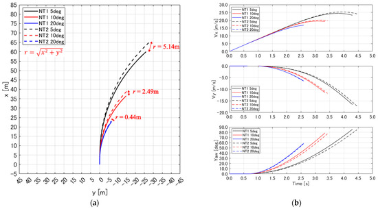
Figure 22.
(a) Trajectories of NT1 and NT2 and (b) velocities and yaw angles of NT1 and NT2.
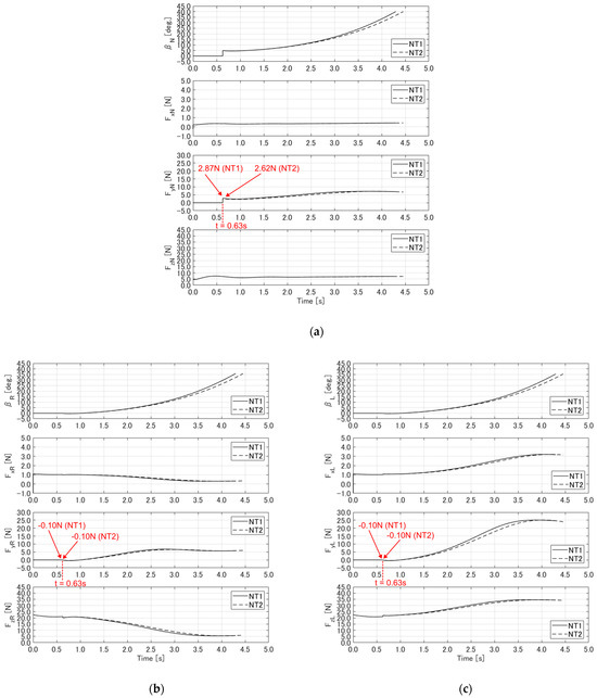
Figure 23.
Comparison of slip angle and tire forces between NT1 and NT2 under steering input of 5 deg.: (a) nose tire, (b) right main tire, and (c) left main tire.
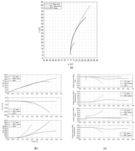
Figure 24.
(a) Trajectories of LT considering aerodynamics, NT1 considering aerodynamics, and NT1; (b) velocities and yaw angles of LT considering aerodynamics, NT1 considering aerodynamics, and NT1; and (c) rolling and yawing moments of LT considering aerodynamics, NT1 considering aerodynamics, and NT1.
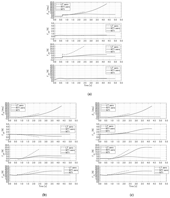
Figure 25.
Comparison of slip angle and tire forces between NT1 aero, NT2 aero, and NT2.: (a) nose tire, (b) right main tire, and (c) left main tire.
5.3.1. Case 1.1: Comparing the Linear Tire Model (LT) with the Nonlinear Tire Model 1 (NT1)
Figure 20a represents the taxiing trajectories of the LT and NT1 when the steering input was set to 5, 10, and 20 deg. Figure 20b shows the time history of the velocity in the -axis direction, the velocity in the -axis direction, and the yaw angle rotation in the body-fixed coordinate system. These results indicate that increasing the steering angle led to a smaller turning radius for both the LT and NT1. However, significant differences were observed between the LT and NT1 in terms of the taxiing trajectory, velocity, and yaw angle. Furthermore, the simulation end times for LT and NT1 are different. The LT simulation ended because the right tire lifted off the ground during a right turn, while the NT1 simulation ended when the front tire’s slip angle exceeded 40 degrees. Those reasons why the simulations ended can be confirmed by the front tire slip angle for NT1 shown in Figure 21a and the transition of the right tire vertical force to zero for LT shown in Figure 21b.
The cause of the significant differences in the taxiing dynamics between the LT and NT1 are discussed using the results of a steering input of 5 deg. Figure 21 shows the slip angle and the tire forces for each tire.
The longitudinal force for each tire showed no significant difference between the LT and NT1. According to Equations (1) and (12), is influenced by . Although a considerable difference in between the right and left tires emerged for the LT and NT1, the difference in was less than 1 N for both models. This result, due to the small values of , , , , and in Table 6 and Table 7, suggests that had a minor impact on the discrepancies in the UAV taxiing dynamics.
Regarding the lateral force for each tire, a significant difference was observed between the LT and NT1. Immediately after the steering input, the nose tire’s lateral force was 8.83 N for LT and 2.87 N for NT1. This difference is attributable to the effect of . After the steering input from s to s, the slip angle remained below 10 deg., and was approximately 7.18 N, with both LT and NT1 having nearly the same values. Therefore, was not the cause of the difference between them. By contrast, the equation for the LT shown in Equation (6) did not include as an input parameter, whereas the equation for NT1 did incorporate , as shown in Equations (13), (15) and (16). This difference resulted in smaller values in the NT1 due to a smaller , whereas the LT did not undergo changes from a smaller because was not included as a parameter. This circumstance accounts for the significant difference in .
These results indicate no significant difference between the LT and NT1 in terms of due to the small values of the friction coefficients , , , , and . However, showed significant differences between the LT and NT1 influenced by whether was included as an input parameter. Indeed, the inclusion or exclusion of significantly impacted the magnitude of the force generated, which subsequently led to a difference in the UAV taxiing dynamics.
5.3.2. Case 1.2: Comparing MF (NT1) with Rankin et al.’s Tire Model (NT2)
Figure 22a shows the taxiing trajectories of the NT1 and NT2, while Figure 22b illustrates the velocity in the -axis direction, the velocity in the -axis direction, and the yaw angle of the UAV in the body-fixed coordinate system. Compared to the results for the LT and NT1 in Figure 20, the results for the NT1 and NT2 in Figure 22 reveal a small difference in the final values.
Figure 23 shows the slip angles and tire forces for each tire under the condition of a 5 deg. steering input. The slip angles and tire forces of each tire at s when the steering input was applied reveal little difference between the NT1 and NT2 for the right and left tires. However, the nose tire exhibited a difference of approximately 0.25 N in lateral force between the NT1 and NT2. Ultimately, this difference in lateral force on the nose tire led to differences in subsequent aircraft dynamics.
Based on these results, the UAV dynamics of the MF and Rankin et al.’s tire model exhibited similar trends.
5.3.3. Case 2.1: Considering Aerodynamics
Figure 24 and Figure 25 show the results when considering aerodynamics. The tire models used were the LT and NT1. For comparison, the results of the NT1 without aerodynamics were also included. In Figure 24a,b, it is evident that the NT1 with aerodynamics improved the straight-line stability, resulting in linear motion. The reason for this is clear in Figure 24c. The NT1 experienced a positive rolling moment due to aerodynamics. The positive rolling moment acted to prevent the aircraft from rolling over. Additionally, the yawing moment due to aerodynamics acted negatively, opposing the right turn. These results indicate that the aerodynamics improved the straight-line stability. Furthermore, Figure 25 shows the forces acting on each tire. It can be seen that the LT with aerodynamics (LT aero) still experienced significant lateral forces. By contrast, the NT1 with aerodynamics (NT1 aero) showed smaller forces acting on each tire compared to the NT1 without aerodynamics, which occurred because the aerodynamics contributed to improving the straight-line stability of the aircraft, thereby reducing the forces on the tires.
6. Conclusions
In our study, we conducted parameter identification experiments to clarify the tire model parameters in fixed-wing UAV taxiing simulations, which have been unclear in previous research. Using the obtained tire model, we also clarified the impact of the tire model on taxiing motion through fixed-wing UAV taxiing simulations.
The parameter identification of the tire model was carried out for both linear and nonlinear tire models using the results of tire force measurement experiments and the method presented in our study. Among the obtained parameters, the lateral force coefficient of the linear tire model differed significantly from those used in crewed aircraft taxiing simulations. Therefore, it is recommended to conduct parameter identification according to the aircraft weight and the tires used when conducting fixed-wing UAV taxiing simulations.
In the taxiing simulations, significant differences in taxiing motion were observed between the linear and nonlinear tire models. The main reason for these differences is whether the load parameter was included in the lateral force tire model equation. Furthermore, in the comparison between the MF and Rankin et al.’s nonlinear tire models, the taxiing motion was almost the same for both models, with slight differences appearing due to the lateral force acting on the nose wheel. From the perspective of tire model construction, Rankin et al.’s tire model has the advantage of being easier to construct than the MF model because only two variables need to be identified: the maximum lateral force and the slip angle at which it occurs.
Finally, a taxiing simulation that included aerodynamics was conducted. The results show that the aerodynamics enhanced the straight-line stability during taxiing, which consequently reduced the forces acting on the tires. By contrast, the linear tire model produced significant lateral forces even when aerodynamics were included because the load parameter was not incorporated into the lateral force model.
The results of our study are valuable in that they identify the parameter values of the tire model based on actual measurements of fixed-wing UAV tires and clarify the differences in taxiing motion due to the tire model and their causes.
Supplementary Materials
The following supporting information can be downloaded at: https://www.mdpi.com/article/10.3390/aerospace11080620/s1, File: TireForceExperimentData.xlsx.
Author Contributions
Conceptualization, H.E.; methodology, H.E.; software, H.E.; formal analysis, H.E.; investigation, H.E.; resources, H.E.; writing—original draft, H.E.; writing—review and editing, D.N. All authors have read and agreed to the published version of the manuscript.
Funding
The research and the APC were funded by the Aerospace Plane Research Center, Muroran Institute of Technology.
Data Availability Statement
Data from the tire force measurement experiment in Section 3 are available upon request.
Conflicts of Interest
The authors declare that they have no conflicts of interest.
Abbreviations
| Mass | |
| Moment of inertia | |
| Gravity | |
| Gravity force in ground-fixed coordinates | |
| Force | |
| UAV engine thrust | |
| Peak value of lateral force | |
| Torque | |
| Velocity | |
| Angular velocity | |
| Distance between two points on the xy-plane | |
| Euler angle around the axis | |
| Euler angle around the axis | |
| Euler angle around the axis | |
| , , | Ground-fixed coordinates |
| , , | UAV body coordinates |
| , , | Tire-fixed coordinates |
| Center of gravity height | |
| Length between nose wheel and center of gravity | |
| Length between main wheel and center of gravity | |
| Main wheel tread width | |
| Tire load | |
| Steering angle | |
| Slip angle | |
| Slip angle at | |
| Stiffness factor of Magic Formula tire model | |
| Shape factor of Magic Formula tire model | |
| Peak factor of Magic Formula tire model | |
| Curvature factor of Magic Formula tire model | |
| Coefficient of MF parameter function | |
| Friction coefficient of longitudinal force | |
| Friction function of longitudinal force | |
| Friction coefficient of lateral force | |
| Friction function of lateral force | |
| Coefficient of tire lateral force | |
| Spring coefficient of vertical force | |
| Damping coefficient of vertical force | |
| , , | Polynomial coefficient of vertical force |
| Displacement in z axis | |
| Tire slip ratio | |
| Main wing area | |
| Main wingspan | |
| Main wing mean aerodynamic chord | |
| Aerodynamic drag coefficient | |
| Aerodynamic lateral force coefficient | |
| Aerodynamic rolling moment coefficient | |
| Aerodynamic yawing moment coefficient | |
| Atmospheric density | |
| Side-slip angle | |
| Subscripts | |
| , , | Direction of body coordinate or tire coordinate |
| Nose tire | |
| Main tire | |
| Right tire | |
| Left tire | |
Appendix A
The coordinate transformation matrices used in Equations (23)–(25) are shown in (A1) through (A3).
References
- Mohsan, S.A.H.; Othman, N.Q.H.; Li, Y.; Alsharif, M.H.; Khan, M.A. Unmanned aerial vehicles (UAVs): Practical aspects, applications, open challenges, security issues, and future trends. Intell. Serv. Robot. 2023, 16, 109–137. [Google Scholar] [CrossRef] [PubMed]
- Rau, J.Y.; Jhan, J.P.; Lo, C.F.; Lin, Y.S. Landslide mapping using imagery acquired by a fixed-wing UAV. In Proceedings of the International Archives of the Photogrammetry, Remote Sensing and Spatial Information Sciences, Zurich, Switzerland, 14–16 September 2011. [Google Scholar] [CrossRef]
- Cobar, M.; Montalvo, C.; Buckner, C. Disaster Response Fixed Wing UAV for Gulf of Mexico Field Campaign. In Proceedings of the AIAA Scitech 2021 Forum, Virtual Event, 11–15 and 19–21 January 2021. [Google Scholar] [CrossRef]
- Boon, M.A.; Drijfhout, A.P.; Tesfamichael, S. Comparison of a fixed-wing and multi-rotor UAV for environmental mapping applications: A case study. Int. Arch. Photogramm. Remote Sens. Spatial Inf. Sci. 2017, XLII-2/W6, 47–54. [Google Scholar] [CrossRef]
- Deng, C.; Wang, S.; Huang, Z.; Tan, Z.; Liu, J. Unmanned aerial vehicles for power line inspection: A cooperative way in platforms and communications. J. Commun. 2014, 9, 687–692. [Google Scholar] [CrossRef]
- BOEING. Statistical Summary of Commercial Jet Airplane Accidents. Available online: https://www.boeing.com/content/dam/boeing/boeingdotcom/company/about_bca/pdf/statsum.pdf (accessed on 5 April 2024).
- Flight Safety Foundation. 2023 SAFETY REPORT. Available online: https://flightsafety.org/foundations-annual-report-highlights-threat-to-aviation-safety-from-eroding-safety-culture/ (accessed on 5 April 2024).
- Flight Safety Foundation, Reducing the Risk of Runway Excursions. Available online: https://flightsafety.org/files/RERR/fsf-runway-excursions-report.pdf (accessed on 5 April 2024).
- Brott, H. A Study of Aircraft Lateral Dynamics & Ground Stability. Master’s Thesis, Rochester Institute of Technology, Rochester, NY, USA, 1998. [Google Scholar]
- Khapane, P.D. Simulation of asymmetric landing and typical ground maneuvers for large transport aircraft. Aerosp. Sci. Technol. 2003, 7, 611–619. [Google Scholar] [CrossRef]
- Rankin, J.; Coetzee, E.; Krauskopf, B.; Lowenberg, M. Nonlinear ground dynamics of aircraft: Bifurcation analysis of turning solutions. In Proceedings of the AIAA Modeling and Simulation Technologies Conference and Exhibit, Honolulu, HI, USA, 18–21 August 2008. [Google Scholar] [CrossRef]
- Rankin, J.; Krauskopf, B.; Lowenberg, M.; Coetzee, E. Operational Parameter study of aircraft dynamics on the ground. J. Comput. Nonlinear Dyn. 2010, 5, 1–11. [Google Scholar] [CrossRef]
- Turbuk, M.C.; Paglione, P. Aircraft ground dynamics modeling, VI National congress of mechanical engineering. In Proceedings of the Campina Grande, Paraiba, Brazil, 18–21 August 2010. [Google Scholar]
- Georgieva, K.; Serbezov, V. Mathematical model of aircraft ground dynamics. In Proceedings of the ICMT 2017—6th International Conference on Military Technologies, Brno, Czech Republic, 31 May–2 June 2017. [Google Scholar] [CrossRef]
- Song, L.; Yang, H.; Yan, X.; Ma, C.; Huang, J. A study of instability in a miniature flying-wing aircraft in high-speed taxi. Chin. J. Aeronaut. 2015, 28, 749–756. [Google Scholar] [CrossRef][Green Version]
- Hou, Y.X.; Guan, Y.; Jia, H. Research on motion characteristics for UAV ground maneuvers. In Proceedings of the 2015 IEEE International Conference on Mechatronics and Automation, Beijing, China, 2–5 August 2015. [Google Scholar] [CrossRef]
- Yin, Q.; Nie, H.; Wei, X. Dynamics and directional stability of high-speed unmanned aerial vehicle ground taxiing process. J. Aircr. 2020, 57, 689–701. [Google Scholar] [CrossRef]
- Yin, Q.; Wei, X.; Nie, H.; Deng, J. Parameter effects on high-speed UAV ground directional stability using bifurcation analysis. Chin. J. Aeronaut. 2021, 34, 1–14. [Google Scholar] [CrossRef]
- Bakker, E.; Nyborg, L.; Pacejka, H.B. Tyre Modelling for Use in Vehicle Dynamics Studies; SAE Technical Paper 870421; Wiley-Intersciece: New York, NY, USA, 1987. [Google Scholar] [CrossRef]
- Wong, J.Y. Theory of Ground Vehicles, 3rd ed.; John Wiley & Sons, Inc.: Hoboken, NJ, USA, 2001. [Google Scholar]
- Mizobata, K.; Minato, R.; Higuchi, K.; Ueba, M.; Takagi, S.; Nakata, D.; Higashino, K.; Tanatsugu, N. Development of a Small-scale Supersonic Flight Experiment Vehicle as a Flying Test Bed for Future Space Transportation Research. Trans. JSASS Aerosp. Technol. Jpn. 2014, 12, Po_3_1–Po_3_10. [Google Scholar] [CrossRef] [PubMed]
Disclaimer/Publisher’s Note: The statements, opinions and data contained in all publications are solely those of the individual author(s) and contributor(s) and not of MDPI and/or the editor(s). MDPI and/or the editor(s) disclaim responsibility for any injury to people or property resulting from any ideas, methods, instructions or products referred to in the content. |
© 2024 by the authors. Licensee MDPI, Basel, Switzerland. This article is an open access article distributed under the terms and conditions of the Creative Commons Attribution (CC BY) license (https://creativecommons.org/licenses/by/4.0/).