A Comparative Study on the Efficiencies of Aerodynamic Reduced Order Models of Rigid and Aeroelastic Sweptback Wings

Abstract

This paper presents the effect of wing elasticity on the efficiency of a nonintrusive reduced order model using a three-dimensional sweptback wing. For this purpose, a computationally low-cost but highly accurate nonintrusive reduced order method is constructed utilizing proper orthogonal decomposition (POD) coupled with radial basis function (RBF) interpolation. The results are evaluated in terms of order reduction and prediction capability of rigid and aeroelastic ROMs. Our results show that compared to the rigid wing, reduced order modeling is more effectively applied to the aeroelastic sweptback wing due to the postponement of flow separation caused by bending–torsion coupling, when the pressure coefficient (Cp) is considered as the output. We further show that for flexible wings, utilizing rigid nodes is not sufficient for presenting the Cp distribution accurately; hence, separate ROMs must be generated for the deformed positions of the nodes. Moreover, the RBF method is also exploited for prediction of the results with direct interpolation of the data ensemble by generating a surrogate model. Finally, the proposed methods are compared in terms of accuracy, computational cost and practicality.

1. Introduction

Static aeroelastic behavior of aerospace structures is an important phenomenon to be considered since it greatly affects the flight performance and hence the design of the structure. However, high-fidelity numerical simulations of aeroelastic problems are computationally costly and demand a large storage capacity. The data acquired from such studies need effective post-processing strategies to gain insight into the physics of the problem and assessment of models with different variables. Therefore, there is an increasing interest in exploiting reduced order models (ROMs) as well as surrogate models among the scientific community to reduce the cost of high-fidelity simulations.

Many techniques are used in reduced order modeling; however, proper orthogonal decomposition (POD) is the most frequently used method in various scientific fields. In this method, the dominant features of the solutions of similar cases are extracted, and the reduced model is constructed by exploiting these dominant features. The POD method produces an optimal linear set of basis vectors that describe the ensemble of data in the optimum way [1]. Then, the reduced order system is represented by the linear superposition of the basis vectors and the corresponding basis coefficients.

To determine the basis coefficients, several methods exist which make ROM modeling intrusive or nonintrusive. In one method, the governing equations of the high-fidelity system can be projected onto the reduced space spanned by basis vectors. The Galerkin method is used frequently as a projection technique in both aerodynamic and aeroelastic studies [2,3,4,5,6]. Since the original equations of the system are modified in this method, such methods are called intrusive. Preserving the underlying physics and the need for access to the governing equations are the main points of intrusive methods. On the other hand, basis coefficients can also be obtained by projecting the available solutions on the basis vectors. By exploiting the basis coefficients at hand, others can be obtained using different methods that make the prediction of solutions possible for different parameters of interest. Since such methods do not depend on the governing equations, they are called nonintrusive methods. The efficiency of intrusive and nonintrusive ROMs in terms of accuracy and computational cost is problem-dependent, and this is investigated in several studies [7,8,9,10,11,12]. Although there are many cases where intrusive methods are declared to give more accurate results, it is known that many industrial applications rely on commercial solvers, such that interference with the source code may not be possible or may be a highly complex task. For such cases, the demand for simple, low-cost but still accurate models can be met by nonintrusive ROMs. Since there is no need to access the governing equations of the problem in nonintrusive ROMs, they enable great flexibility in practical applications.

For the construction of POD-based nonintrusive ROMS, several interpolation methods can be adopted for the evaluation of basis coefficients such as cubic spline interpolations [13,14,15,16,17,18], radial basis function (RBF) methods [16,19,20,21,22,23], Kriging or Kriging-based interpolation methods [21,24,25,26,27] and other interpolation methods [10,18,28,29]. The interpolated coefficients are then exploited for the prediction of data for the relevant flow variable (angle of attack, Mach number, etc.) [13,14,15,16,28], geometric variable (chord, thickness, etc.) [10,16,25,30], structural variable (stiffness, density, etc.) or flight condition (altitude, load factor, etc.). For unsteady analyses, time and frequency can also be varying parameters [19,20,22]. In some cases, different kind of variables, such as a flow and a structural variable, are investigated together [21,24].

In the static aeroelastic analysis of aircraft structures, ROM techniques can be applied to either the fluid part or the structural part, as well as to both parts, in order to reduce the order of the overall model. The expectation from a reduced model is that it approximates the results corresponding to a different input variable set accurately with less computational time. Lindhorst et al. replaced the CFD solver in the aeroelastic coupling scheme with a ROM performing static as well as transient analyses of an airfoil [31]. For time independent problems, the ROM is constructed by coupling POD with the radial basis function artificial neural network (RBF-ANN) method. A similar study is also conducted for wing analysis [32]. In the study of Ripepi et al., a ROM with POD and Isomap methods, in both intrusive and nonintrusive frameworks, is used to predict static aeroelastic loads to exploit in multidisciplinary optimization [33]. Similarly, a ROM based on the Volterra series method is used for modeling the aerodynamic part for the static aeroelastic response of composite plates as well as the AGARD 445.6 and the HiReNASD wing configurations [34]. On the other hand, in the study of Xie et al., the structural model in the aeroelastic analysis of a wing is represented by a ROM [35]. A ROM is obtained by regression analysis from load cases and corresponding deformations, and then it is coupled with vortex lattice aerodynamics to obtain the static aeroelastic behavior of the wing. In the study of Berthelin et al., surrogate models are constructed for the aerodynamic and the structural disciplines separately using POD with Gaussian Process interpolation [36].

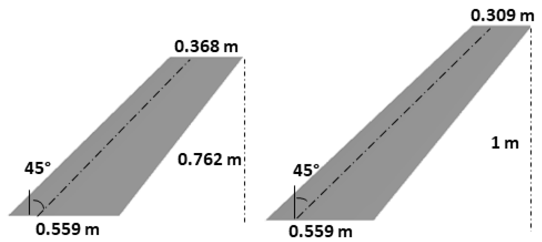
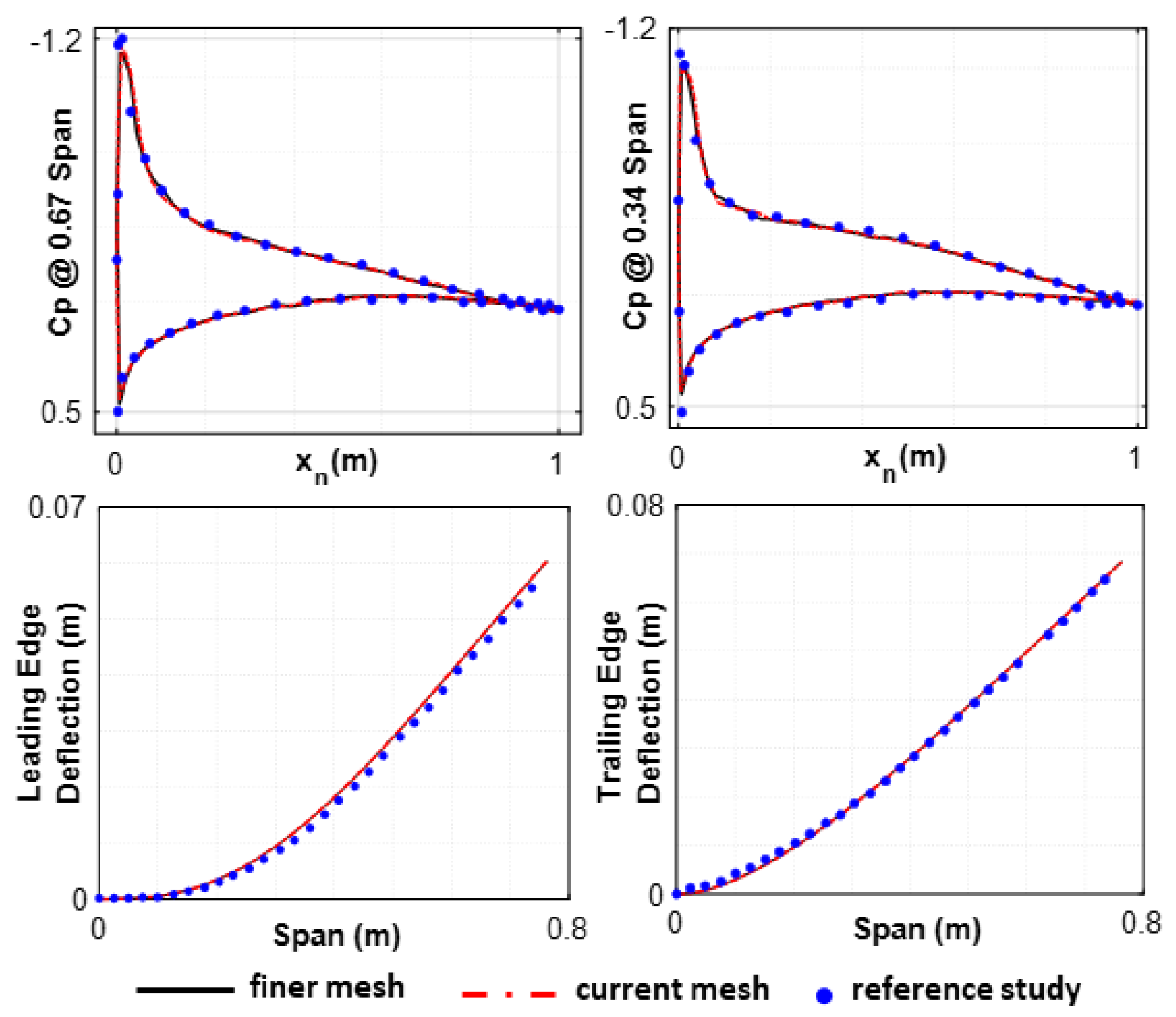
This study presents nonintrusive POD-based ROMs for rigid and aeroelastic sweptback wing configurations which require aerodynamic and static aeroelastic analysis of the 3-dimensional wing for varying flow conditions parameterized by the angle of attack and the Mach number. The effectiveness of the application of the POD-based ROM is compared for both configurations, and conclusions are inferred with regard to the effect of the bending–twisting coupling of the sweptback wing configuration on decreasing the number of POD modes to be included in the ROM constructed compared to the rigid wing configuration. The effect of bending–twisting coupling of sweptback wing configurations on reducing the effective number of POD modes compared to rigid sweptback wing configurations is not studied in the literature. Nonintrusive POD-based ROMs are constructed by exploiting the results of high-fidelity CFD analysis with Navier–Stokes equations for the rigid wing and two-way fluid structure interaction analysis for the aeroelastic wing with high-fidelity CFD analysis on the aerodynamic side and 3D finite element analysis on the structure side. Both aerodynamic and structural disciplines are included together under the nonintrusive POD-based ROM framework to reconstruct the resultant aerodynamic and structural metrics of the wing. For the evaluation of the prediction capability of the method, Cp distributions are predicted for different angle of attacks and Mach conditions for both rigid and aeroelastic wings. Contrary to the rigid wing, the effect of changes in the positions of the nodes of the aeroelastic wing due to the deflection of the wing is also investigated in this study. In this respect, for the prediction of the Cp distribution by the POD-based ROM, converged nodal positions of the wing surface obtained from the high-fidelity static aeroelastic analysis are also taken into account while constructing the ROM. For the evaluation of deformed nodal positions, another POD-based ROM is generated, and Cp distribution and wing deflection predictions are made utilizing the ROM generated for the deformed nodal positions of the aeroelastic wing. It is noted that, especially for flexible wings, it is necessary to generate a separate ROM for the deformed positions of the nodes in order to obtain accurate variation of the Cp distribution in the wing. The separate ROM generated for the deformed positions of the nodes also allows the calculation of the deformation of the wing as a by-product. In addition, von Mises stress distribution in the aeroelastic wing is obtained by constructing a ROM utilizing the high-fidelity solutions of static aeroelastic analysis. Moreover, in the present study the RBF method is adopted as an interpolation method coupled with the POD method for the CFD analysis of the rigid wing and the static aeroelastic analysis of the aeroelastic wing. In addition, the RBF method is also exploited for prediction of the results with direct interpolation of the data ensemble in a comparative manner.

The rest of the article is organized as follows. In Section 2, the test wing is introduced, and the methodologies of high-fidelity CFD and static aeroelastic analyses are presented. Section 2 also explains the POD and RBF techniques implemented. Section 3 presents the reduced order model constructed by exploiting small numbers of POD modes for both rigid and aeroelastic sweptback wing configurations, and the results are compared with the high-fidelity results and discussed accordingly. In Section 4, results of the intermediate parameters that do not exist in the original data set are predicted, exploiting the reduced order models constructed. In addition, at the end of this section, instead of the reduced order model, a surrogate model is exploited using the RBF technique for the same purpose. Finally, the results are compared in terms of accuracy, computational cost and practicality.

2. Methodology

2.1. High-Fidelity Full Order Models of the Rigid and Aeroelastic Sweptback Wing Configurations

In this study, a 3D sweptback wing configuration is investigated for both rigid and aeroelastic configurations. CFD analysis is conducted for the rigid wing using the commercial solver Ansys Fluent Release 21.2 [37]. For the aeroelastic case, Ansys Fluent is coupled with Ansys Mechanical Release 21.2 [38] via the system coupling tool to perform two-way static aeroelastic analysis, as demonstrated in Figure 1.

Static aeroelastic analysis is an iterative solution process during which aerodynamic loads are interpolated between nonconformal meshes on either side of the fluid–solid interface. Dynamic mesh is defined at the fluid–solid interface using the diffusion-smoothing method, such that interior nodes are moved with the deforming boundary and the number of nodes and their connectivities does not change. The solutions obtained from the CFD analysis of the rigid wing and the two-way static aeroelastic analysis of the elastic wing are considered as high-fidelity results since they reflect real-life phenomena with a significant degree of accuracy.

The baseline model used in this study is the AGARD 445.6 wing [39], which is a well-known test case for aeroelastic problems. It is a swept wing with an NACA 65A004 airfoil [39]. In the current study, the span of the baseline AGARD 445.6 wing is increased by about 30%, which leads to a decrease in the stiffness of the wing, making the static aeroelastic effects more remarkable. The dimensions of the baseline and the elongated AGARD 445.6 wing and the first four natural frequencies are given in Figure 2 and

Table 1. Comparison of the modal frequencies.

	1st Bending Mode (Hz)	1st Torsion Mode (Hz)	2nd Bending Mode (Hz)	2nd Torsion Mode (Hz)
AGARD 445.6	9.599	39.165	48.348	91.545
AGARD 445.6 with 1 m Span	5.894	25.607	36.753	62.420

, respectively.

The decision on the proper CFD mesh density to be used in the AGARD 445.6 wing with elongated span was made after a comparative study. The maximum wing deflection and the 3D C_L results obtained with the current mesh and finer mesh used in this study are compared in

Table 2. Results of different mesh cases.

	Element Number	Node Number	CL	Maximum Wing Deflection (m)
Finer Mesh	2,921,285	726,109	0.2668	0.0683
Current Mesh	2,310,158	570,659	0.2670	0.0683

.

It is noted that the differences between the current and the finer meshes in terms of 3D C_L and maximum wing deflection results are insignificant. In addition, the Cp distribution and the edgewise deflections obtained from the static aeroelastic analysis of the baseline AGARD 445.6 wing are compared with the reference study [40] for different mesh densities in Figure 3.

The comparative study presented in Figure 3 shows that the mesh case represented as the ‘current mesh’ is able to predict the results obtained by Cai et al. [40] accurately. Therefore, the ‘current mesh’ is also adapted for the elongated AGARD 445.6 wing. In the CFD model of the elongated AGARD 445.6 wing, the fluid domain is made from a half cylindrical prism cut by the symmetry plane, and the wing is placed inside the half cylindrical prism, as shown in Figure 4.

The far-field boundary condition is defined on the surfaces of the prism except the surface where the root of the wing is located. The symmetric boundary condition is defined on this surface. Figure 5 shows a detailed view of the root section. For the wing surface, no slip wall condition is defined. Finer mesh is applied on the edges of the wing to obtain an accurate airflow on the wing and also to avoid convergence issues. In addition, the mesh at the zone near the wall of the wing is also refined to keep y+ below 1 at the boundary layer.

In the current mesh, there are 20,366 nodes on the surface of the wing in total, and each of these nodes is used to obtain the data to create a snapshot matrix. For the flow conditions, compressible and viscous flow with the SST k-w turbulence model assumption are used.

2.2. Reduced Order Models of the Rigid and the Aeroelastic Sweptback Wing Configurations

2.2.1. Proper Orthogonal Decomposition

POD is an effective statistical tool that is able to extract dominant features from a large data set. The data set can be obtained from either the results of experiments or simulations for one or more variables of interest. Exploiting the data set, a snapshot matrix of $\mathrm{Z}\in {\mathbb{R}}^{\mathrm{n}\mathrm{x}\mathrm{m}}$ is created for the ‘m’ number of results of a system for a changing parameter and the ‘n’ number of nodes or points where the data are taken. It is common to subtract from each row of Z the mean value of that row, to create a modified snapshot matrix. Defining $\stackrel{\sim }{{\mathrm{z}}_{\mathrm{k}}}={\displaystyle \frac{1}{\mathrm{m}}}\sum _{\mathrm{i}=1}^{\mathrm{m}}{\mathrm{z}}_{\mathrm{i}}$, as the mean of the k^th row, the mean vector $\stackrel{\sim }{\mathrm{z}}$ is formed. Then, the modified snapshot matrix is constructed as

$${\left\{\overline{\mathrm{z}}\right\}}_{\mathrm{i}}={\left\{\mathrm{z}\right\}}_{\mathrm{i}}-\stackrel{\sim }{\mathrm{z}},\hspace{1em}\hspace{1em}\hspace{1em}\mathrm{i}=\mathrm{1,2},\dots ,\mathrm{m}$$

(1)

where m is the total number of snapshots.

The aim of the POD method is to first extract the optimal orthogonal basis vectors or the POD modes from the sampled parameter space, the snapshot matrix. From these basis vectors, the first ${\mathrm{m}}_{\mathrm{s}}<\mathrm{m}$ modes that contain sufficient information provided by the snapshots are chosen. Singular value decomposition (SVD) or method of snapshots (MOS) techniques can be used for this purpose. When the snapshot matrix has a few snapshots but an excessive number of nodes (n >> m), the method of snapshots is an effective alternative that can be applied. In this method, eigenvectors and eigenvalues of the covariance matrix (${\overline{\mathrm{Z}}}^{\mathrm{T}}\overline{\mathrm{Z}})$ are determined. The covariance matrix has a size of m × m, which is much less than the original snapshot matrix and therefore easier to handle.

In this method, POD basis vectors are calculated as

$${\mathrm{U}}_{\mathrm{j}}={\displaystyle \frac{1}{{\mathrm{s}}_{\mathrm{j}}}}{\sum }_{\mathrm{l}=1}^{\mathrm{m}}{\left({\mathrm{V}}_{\mathrm{j}}\right)}_{\mathrm{l}}{\mathrm{z}}_{\mathrm{l}}\hspace{1em}\hspace{1em}\hspace{1em}\mathrm{j}=1,2,\dots ,\mathrm{m}$$

(2)

where s is the square root of eigenvalues, V stands for the eigenvectors and m is the number of snapshots. Similar to the SVD method, the eigenvalues of the covariance matrix quantify the importance of the basis vectors and enable the determination of the number of dominant modes,${\mathrm{m}}_{\mathrm{s}}$. The percentage of the captured energy of the modes is calculated as

$$\%\mathrm{E}={\displaystyle \frac{\sum _{\mathrm{i}=1}^{{\mathrm{m}}_{\mathrm{s}}}{\mathrm{s}}_{\mathrm{i}}}{\sum _{\mathrm{i}=1}^{\mathrm{m}}{\mathrm{s}}_{\mathrm{i}}}}$$

(3)

After obtaining the modes exploiting either the SVD or the method of snapshots, the solution at a particular parameter that already exists in the initial sample data is reconstructed as

$${\mathrm{z}}_{\mathrm{j}}^{\mathrm{r}\mathrm{c}}=\stackrel{\sim }{\mathrm{z}}+{\sum }_{\mathrm{i}=1}^{{\mathrm{m}}_{\mathrm{s}}<\mathrm{m}}{\mathrm{a}}_{\mathrm{j}\mathrm{i}}{\mathrm{U}}_{\mathrm{i}} \mathrm{j}=1,2,\dots ,\mathrm{m}$$

(4)

where ${\mathrm{z}}^{\mathrm{r}\mathrm{c}}$ denotes the reconstructed result. Equation (4) gives the solution as the linear combination of a set of orthonormal basis vectors and the corresponding coefficients ${\mathrm{a}}_{\mathrm{j}\mathrm{i}}$, which are also referred to as basis/scalar/projection/POD coefficients. The POD coefficients are obtained by projecting the solutions onto the POD modes as

$${\mathrm{a}}_{\mathrm{j}\mathrm{i}}={\mathrm{z}}_{\mathrm{j}}^{\mathrm{T}}{\mathrm{U}}_{\mathrm{i}} \mathrm{j}=1,2,\dots ,\mathrm{m};\mathrm{i}=1,2,\dots ,{\mathrm{m}}_{\mathrm{s}}$$

(5)

Equation (4) is used to obtain the results of the system at a desired parameter for which a snapshot has already been calculated; however, it can also be used predict the solutions at intermediate parameters in the sampling space by creating a surrogate model having the parameters as input and the POD coefficients as output. In this study, the RBF method is adopted for this purpose.

2.2.2. Regression Model for the Interpolation

As mentioned in the introduction, there are many regression techniques utilized to provide a relationship between input variables and the outcomes. In particular, RBFs are suitable due to their flexibility, convenience and accuracy when applied to scattered multi-dimensional data sets [41]. Therefore, the RBF-based interpolation is considered to be appropriate for this study. The RBF-based interpolation model is a linear combination of basis functions evaluated at the Euclidean distance between the point x (at which the interpolation is made) and all the other points in the known data set. The RBF model does not require regular data for accurate approximation; in particular, it is suitable for scattered data. RBF approximation of a function is built as

$${\mathrm{f}\left(\mathrm{x}\right)}_{\mathrm{k}}=\sum _{\mathrm{i}=1}^{\mathrm{m}}{\mathsf{\beta }}_{\mathrm{i}}\mathsf{\varphi }\left(‖\mathrm{x}-{\mathrm{x}}_{\mathrm{i}}‖\right)\hspace{1em}\hspace{1em}\hspace{1em}\mathrm{k}=1,\dots \mathrm{n}$$

(6)

where m is the number of data points, x_is are the values at data points, ϕ is the chosen RBF and ‖.‖ is used to denote the Euclidean norm. In the current study, the multiquadric basis function given in Equation (7) is used as the RBF.

$$\mathsf{\varphi }=1+\sqrt{\mathrm{c}{‖\mathrm{x}‖}^2}$$

(7)

where the constant c > 0 is called the shape parameter. In Equation (6), β_is are unknown coefficients to be found by making use of the existing data. Denoting the training data vector as f, the coefficient vector as β and the interpolation matrix as ϕ, one can express the relation between them as

$$\mathrm{f}=\mathsf{\varphi }\mathsf{\beta }$$

(8)

• where ${\mathrm{f}}_{\mathrm{k}}=\left\{\begin{array}{c}{\mathrm{f}}_1\\ {\mathrm{f}}_2\\ \begin{array}{c}⋮\\ {\mathrm{f}}_{\mathrm{m}}\end{array}\end{array}\right\}{\mathsf{\beta }}_{\mathrm{k}}=\left\{\begin{array}{c}{\mathsf{\beta }}_1\\ {\mathsf{\beta }}_2\\ \begin{array}{c}⋮\\ {\mathsf{\beta }}_{\mathrm{m}}\end{array}\end{array}\right\}{\mathsf{\varphi }}_{\mathrm{k}}=\left[\begin{array}{cc}\begin{array}{cc}{\mathsf{\varphi }}_{11}& {\mathsf{\varphi }}_{12}\\ {\mathsf{\varphi }}_{21}& \ddots \end{array}& \begin{array}{cc}\dots & {\mathsf{\varphi }}_{1\mathrm{m}}\\ \ddots & {\mathsf{\varphi }}_{2\mathrm{m}}\end{array}\\ \begin{array}{cc}⋮& \ddots \\ {\mathsf{\varphi }}_{\mathrm{m}1}& \dots \end{array}& \begin{array}{cc}\ddots & ⋮\\ \dots & {\mathsf{\varphi }}_{\mathrm{m}\mathrm{m}}\end{array}\end{array}\right] ,\mathrm{k}=1,\dots \mathrm{n}$
• and ${\mathsf{\varphi }}_{\mathrm{i}\mathrm{j}}=\mathsf{\varphi }\left(‖{\mathrm{x}}_{\mathrm{i}}-{\mathrm{x}}_{\mathrm{j}}‖\right)$. Once the equation is solved for undetermined coefficients β, the approximation function f(x) can be evaluated for any data points which are not in the original data set.

Coupled with the POD method, the RBF interpolation method can be used to predict the solutions at intermediate parameters that are not sampled in the original snapshot matrix. However, it is also possible to perform RBF interpolation directly on the snapshot matrix for the same purpose. When data reduction is not the main concern, this approach could also be adopted. In this study, we compare the two approaches in terms of accuracy and computational cost.

3. Reconstruction of Results Based on the POD Method

In the current study, two flow parameters, angle of attack (AOA) and Mach number (M), are taken as variables. The snapshots are taken in the subsonic regime between 0.55 and 0.85 Mach with a uniform interval of 0.05 Mach and between 1° and 5° AOA with a uniform interval of 0.5°, leading to 63 snapshots in total. Based on the high-fidelity analysis results obtained for the input data comprising the AOA and M, the POD and RBF methodologies are applied on the rigid and aeroelastic wing configurations from the results of the CFD analysis and 2-way coupled CFD with static structural analysis, respectively. Cp distribution is taken as the aerodynamic output for both rigid and aeroelastic wing. Moreover, for the aeroelastic wing, displacement and von Mises stress distributions are also determined as the structural output.

The results of the reduced order model are compared with full order solutions for the variables that are not contained in the initial snapshot matrix utilizing the R² error, root mean squared error (RMSE) and normalized root mean squared error (NRMSE) metrics defined in Equation (9).

$$\begin{gathered} {\mathrm{R}}^2=1-{\displaystyle \frac{{\sum _{\mathrm{i}=1}^{\mathrm{N}}({\mathrm{z}}_{\mathrm{a},\mathrm{i}}-{\mathrm{z}}_{\mathrm{p},\mathrm{i}})}^2}{{\sum _{\mathrm{i}=1}^{\mathrm{N}}({\mathrm{z}}_{\mathrm{a},\mathrm{i}}-\overline{{\mathrm{z}}_{\mathrm{a}}})}^2}} \\ \mathrm{R}\mathrm{M}\mathrm{S}\mathrm{E}=\sqrt{{\displaystyle \frac{{\sum _{\mathrm{i}=1}^{\mathrm{N}}({\mathrm{z}}_{\mathrm{a},\mathrm{i}}-{\mathrm{z}}_{\mathrm{p},\mathrm{i}})}^2}{\mathrm{N}}}}\hspace{1em}\mathrm{N}\mathrm{R}\mathrm{M}\mathrm{S}\mathrm{E}={\displaystyle \frac{\mathrm{R}\mathrm{M}\mathrm{S}\mathrm{E}}{{{(\mathrm{z}}_{\mathrm{a},\mathrm{i}})}_{\mathrm{m}\mathrm{a}\mathrm{x}}-{{(\mathrm{z}}_{\mathrm{a},\mathrm{i}})}_{\mathrm{m}\mathrm{i}\mathrm{n}}}} \end{gathered}$$

(9)

where z_a,i, z_p,i and $\overline{{\mathrm{z}}_{\mathrm{a}}}$ stand for the actual, predicted and average of the actual values of output (Cp, wing displacement and von Mises stress), respectively, i is the node number and N is the total number of nodes.

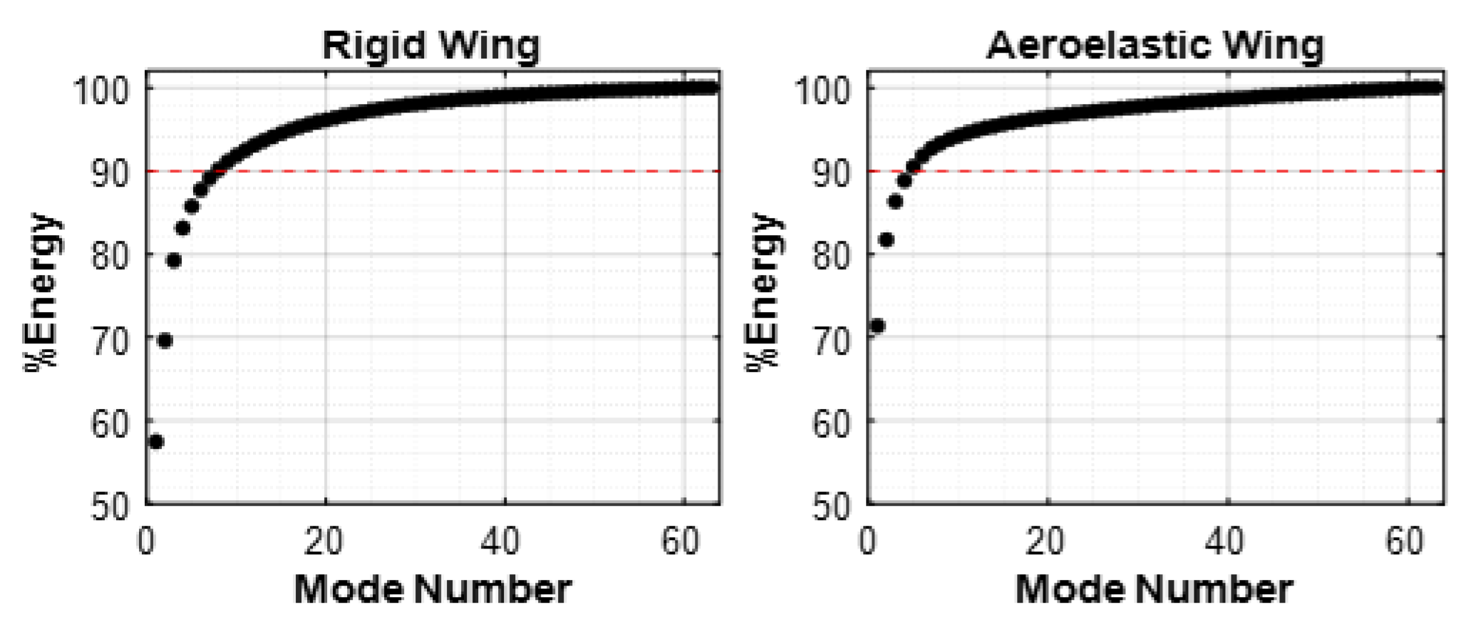
A reduced order model is constructed both for the rigid and aeroelastic wing configurations using POD. By applying the MOS technique, the energy of the system captured by each mode and the corresponding basis functions are obtained. It should be noted that since the number of nodes on the surface of the 3D wing is far more than the number of variables, MOS is computationally much faster; therefore, in the current study the MOS technique is used. For the rigid wing, 1 mode captures 57.48% of the energy, while for the aeroelastic wing the percentage increases to 71.38%. The results show that in order to reach at least 90% of the energy of the system, 8 modes are required for the rigid wing and 5 modes are required for the elastic wing. The accumulated energies for Cp distributions with respect to mode number are given in Figure 6.

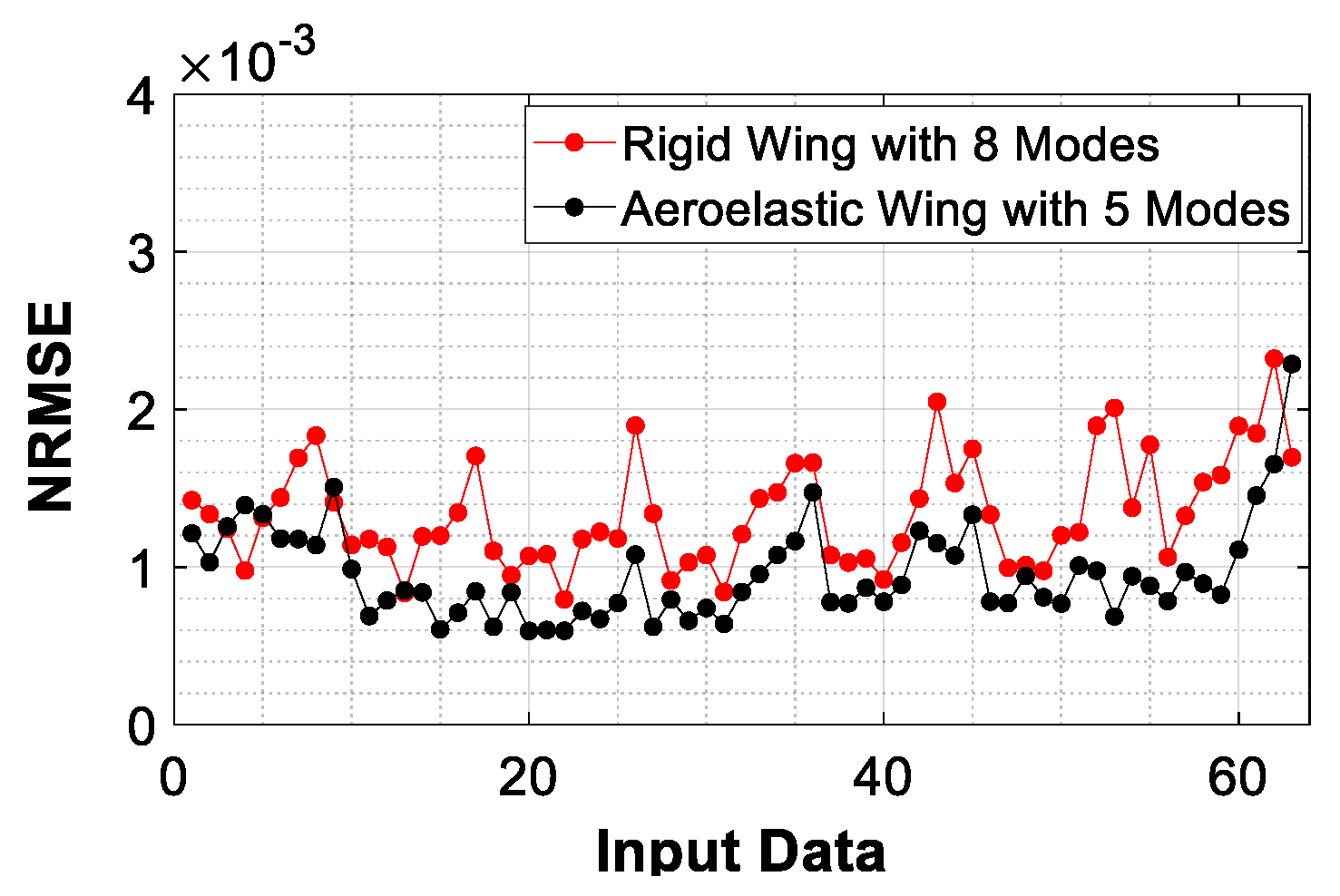
By exploiting these modes, Cp results for each 63 AOA and Mach number pair in the snapshot domain are reconstructed; in Figure 7, NRMSE values are presented for each reconstructed result.

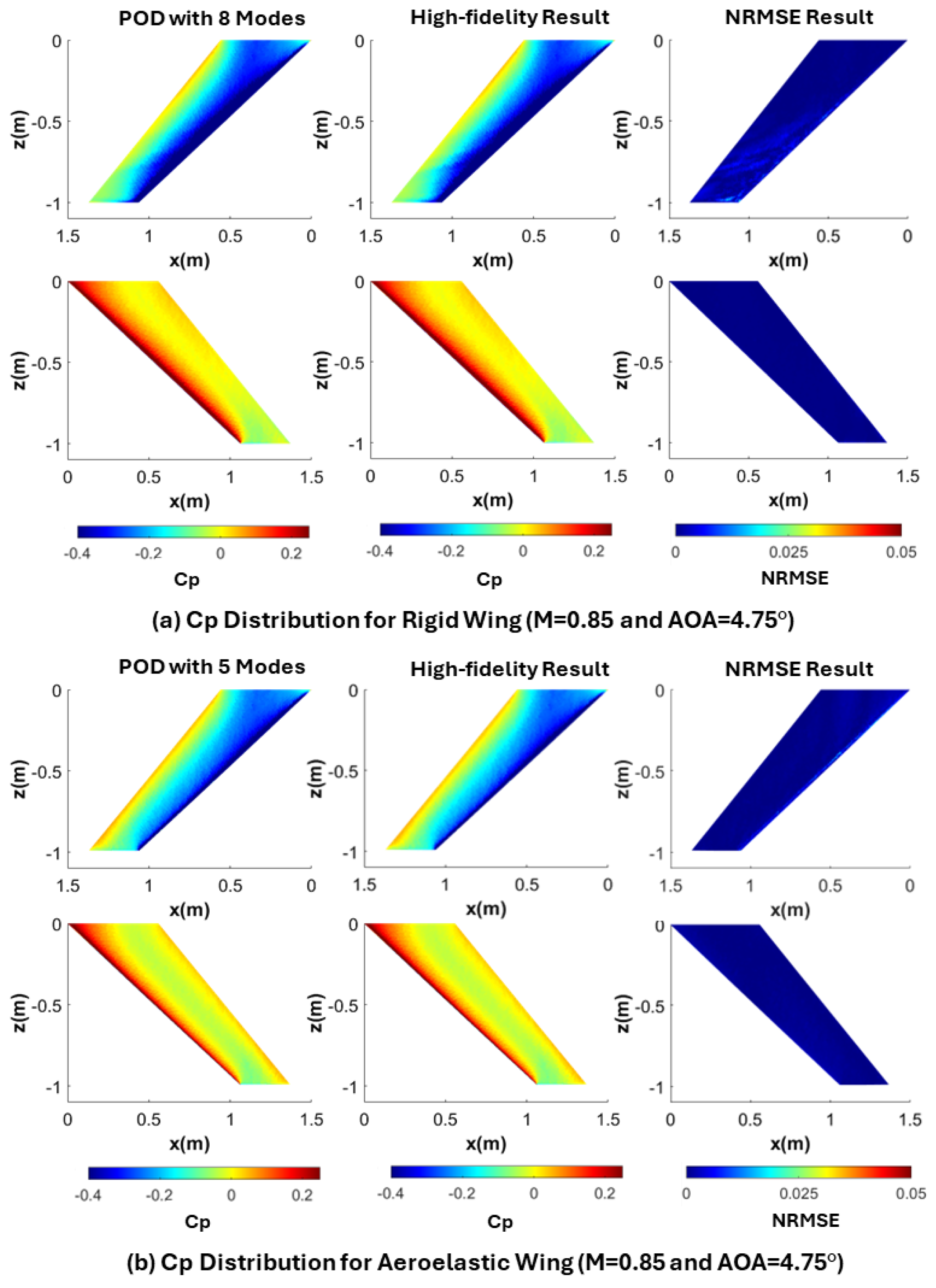
As is clearly seen in Figure 7, NRMSE values of the reconstructed results, with 8 modes for the rigid wing and 5 modes for the aeroelastic wing, are very close to zero, which proves the accuracy of the results. It should also be noted that NRMSE results are lower for the aeroelastic wing for the majority of the flow cases. To verify that 8 and 5 modes are sufficient to reflect the actual results for the rigid and aeroelastic wings, respectively, Cp distributions of the least accurate flow condition are compared with the high-fidelity Cp in Figure 8.

Figure 8 shows that even for the least accurate flow condition in the data domain, 8 modes and 5 modes give highly accurate results for rigid and aeroelastic wings, respectively. Hence, in Section 4 for the purpose of predicting Cp distributions, 8 and 5 modes are used in the POD-based reduced order models for the rigid and the aeroelastic wings, respectively. It should also be noted that in the aeroelastic wing case, since the locations of the nodes also change due to deflection of the wing, contrary to the rigid wing, each analysis case has its own node positions. Therefore, separate snapshot matrices for the x, y and z positions of the nodes are constructed to display the Cp distributions accurately. The MOS technique is also applied on these snapshot matrices. In this case, the first mode captures 97.1% of energy for the x position, 99.5% of energy for the y position and 97.4% of energy for the z position of the nodes. Hence, it is concluded that using only 1 mode is sufficient for the reconstruction of the nodal positions, indicating a significant reduction of order. Cp distributions for the aeroelastic wing are presented with their corresponding node positions whose ROM is generated using only 1 mode. Moreover, deflection of the wing can also be obtained from the position of the nodes as a by-product. 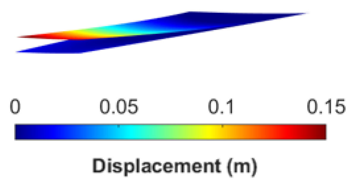Figure 9 shows the reconstructed displacement results using the POD-based ROM at M = 0.85 and 5° AOA for the aeroelastic wing. The rigid wing is also shown in this figure for comparison purposes.

The maximum displacement obtained by the reduced order solution with 1 mode is 0.1584 m, while the full order static aeroelastic analysis gives 0.1580 m for the M = 0.85 and 5° AOA flow condition. With 1 mode, it has been possible to obtain a very accurate maximum displacement result.

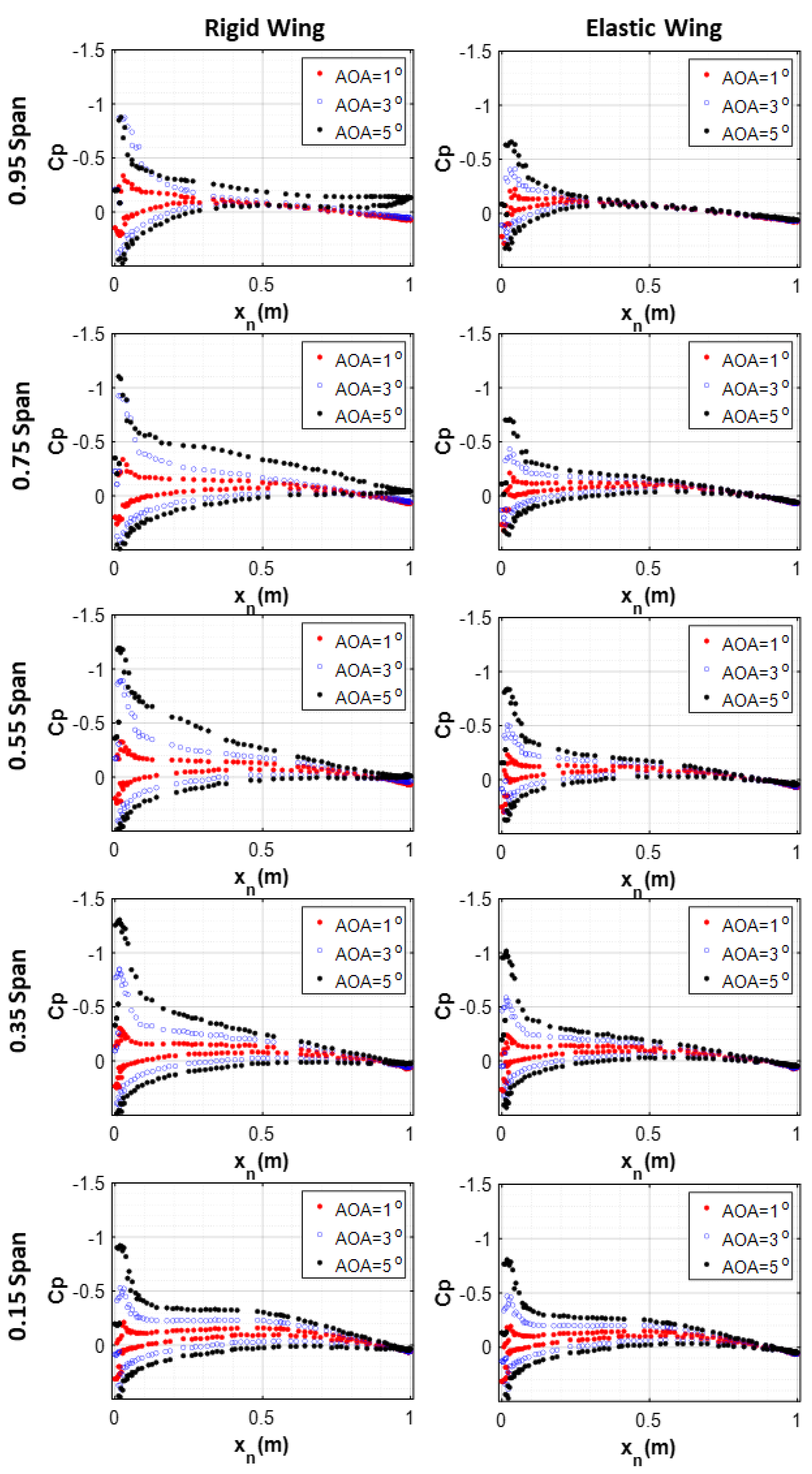
The reason for requiring a lower number of modes to reach 90% of the energy for the aeroelastic wing is attributed to the regular pattern that is obtained in the Cp distribution for the aeroelastic wing. However, for the rigid wing, the pattern starts to be disrupted as the AOA increases. The disruption of the Cp variation is shown in Figure 10, which compares the chordwise Cp distributions for the rigid and aeroelastic wings for M = 0.85 and 3 different AOAs (1°, 3° and 5°) at different span locations.

The span locations are displayed in Figure 11. The nodes which are used for the comparison of the results for different cases are taken from sectional regions within a 0.004 m interval from the given chordwise section.

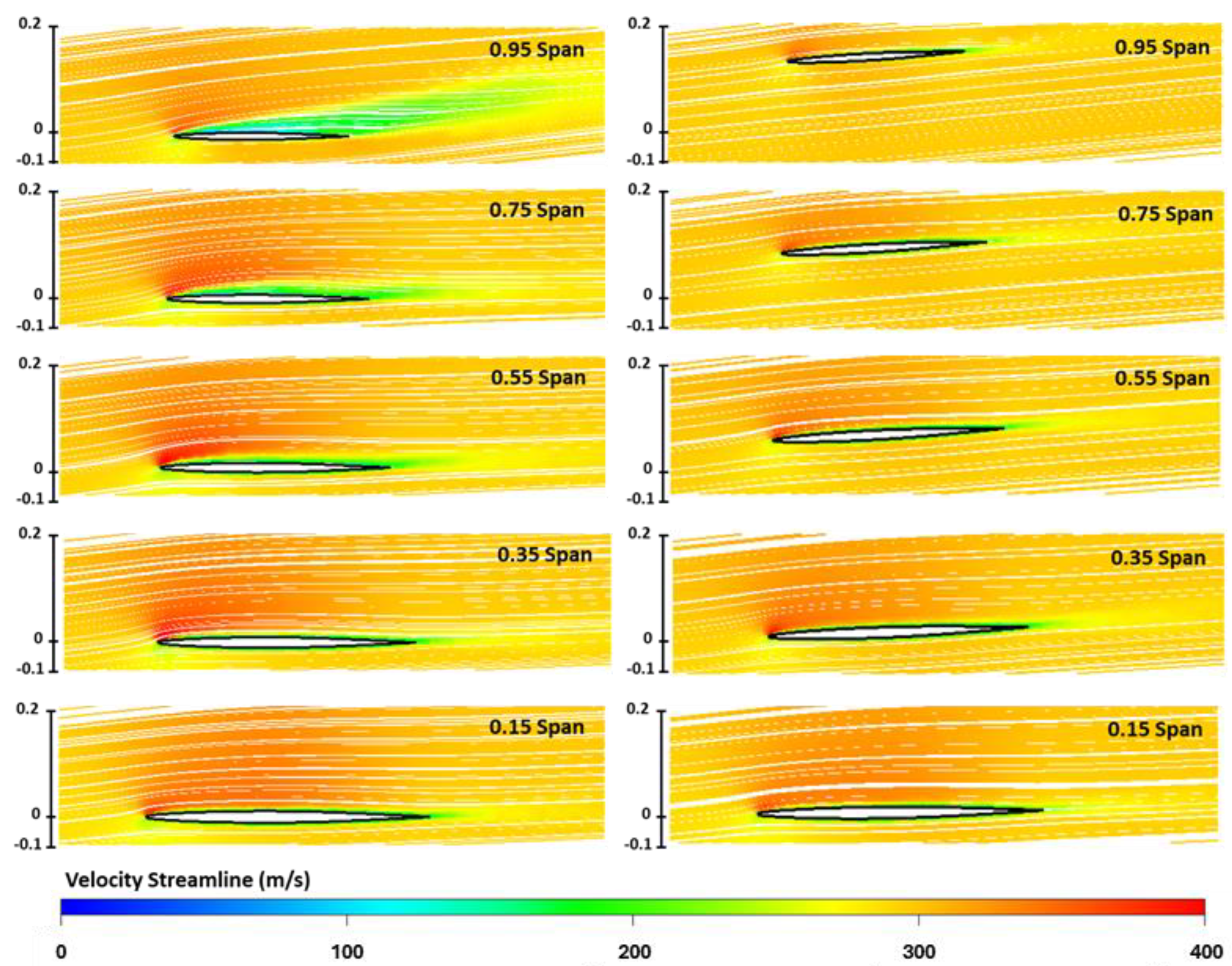
Figure 10 shows that for the rigid wing, at a higher AOA such as 5°, the Cp distribution ceases to follow a pattern like the aeroelastic wing. Figure 12 displays the streamlines around the rigid and the aeroelastic wings for the 5° AOA case at the five different sections of the wing shown in Figure 11.

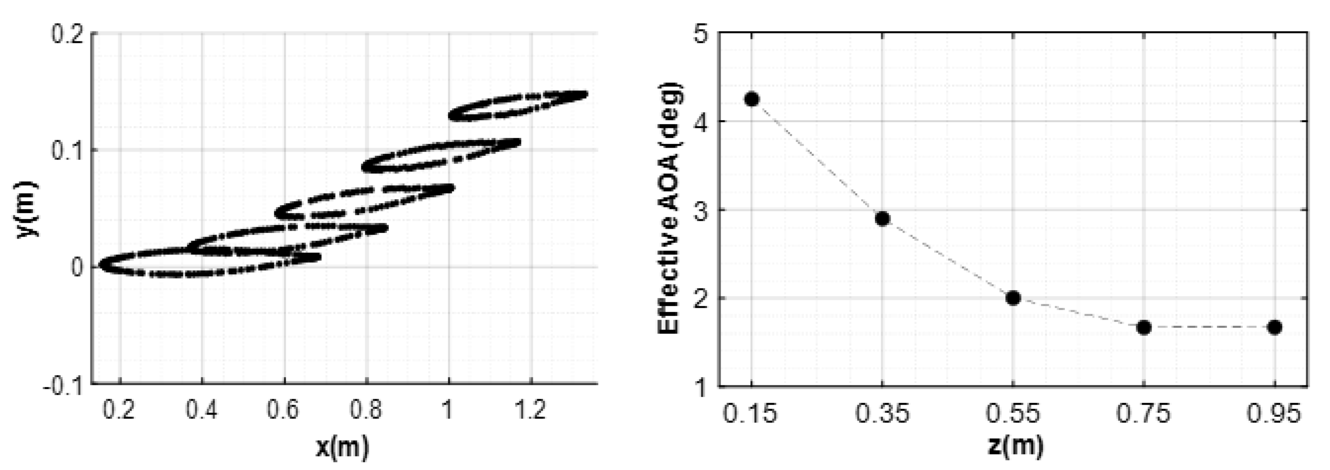
As seen in Figure 12, for the rigid wing, at 5° AOA flow starts to separate, whereas it is still attached for the aeroelastic sweptback wing. The separation progressively increases from wing root to the wing tip. It is worth noting that the wing concerned has a relatively thin airfoil which gets thinner towards the tip, making it more prone to separation. The streamlines exhibit a pronounced upward deflection near the leading edge. However, for the aeroelastic sweptback wing streamlines are relatively undisturbed and follow the airfoil smoothly without a pronounced separation. The reason for this behavior is attributed to the decrease in the effective AOA due to the inward twist of the aeroelastic sweptback wing due to bending. The decrease in the effective AOA at different sections of the aeroelastic wing (Figure 11) at the same flow condition (M = 0.85 and AOA = 5°) is shown in Figure 13.

As a typical behavior of wings with sweptback geometry, when the aeroelastic wing bends, the effective AOA at a wing section decreases due to the bending–torsion coupling. The bending deformation induces twisting of the wing sections as shown in Figure 13. The twisting of the wing due to bending leads to a decrease in the effective AOA in the wing sections, ceasing the flow separation. As seen in Figure 13, the outboard sections of the aeroelastic sweptback wing twist inward to a greater extent compared to the inboard sections. For the rigid angle of attack case of 5°, in almost half of the wing in the outboard sections, the effective angle of attack is less than 2°. Since there is no drastic change in the Cp distribution for the aeroelastic sweptback wing as there is with the rigid wing, a smaller number of modes can capture the system behavior easily as, and this accounts for more efficient reduced order modeling for the aeroelastic sweptback wing compared to the rigid wing. In the following section, the prediction ability of the ROMs is evaluated for both configurations.

4. Prediction of Results Based on the Coupled POD-RBF Method for the Rigid and Aeroelastic Sweptback Wings

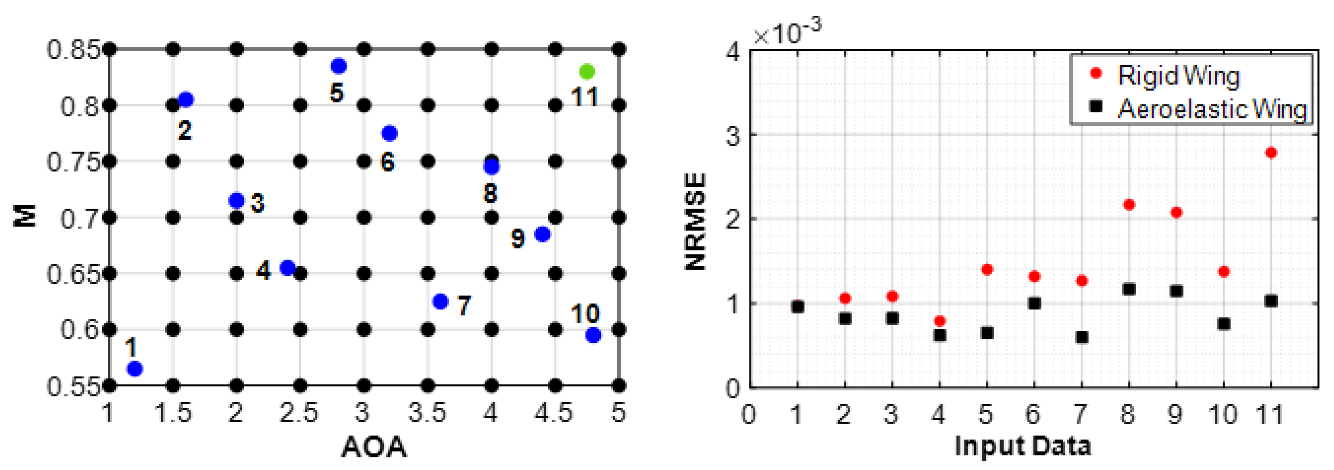
In this section, the POD-based reduced order models are coupled with the RBF interpolation method to predict the results at intermediate variables that do not exist in the original data ensemble. For this purpose, Latin hypercube sampling (LHS) is adopted to decide on 10 flow conditions in the selected interval. The LHS method divides the interval into subintervals and guarantees that each of them has a single sample. Therefore, LHS is able to provide better uniformity compared to random sampling, even if the samples are selected randomly. In Figure 14, parameter pairs used for the assessment of the POD-RBF model as well as the NRMSE results for each case are shown. Parameter pairs shown as black dots are the data samples from the snapshot matrix, whereas the 10 parameter pairs derived from the LHS are shown as blue dots. Moreover, an intermediate flow condition at high M and AOA (M = 0.83 and AOA = 4.75°) is also added to make the effect of deflection of the aeroelastic wing more visible. This data point is shown as the green dot in Figure 14.

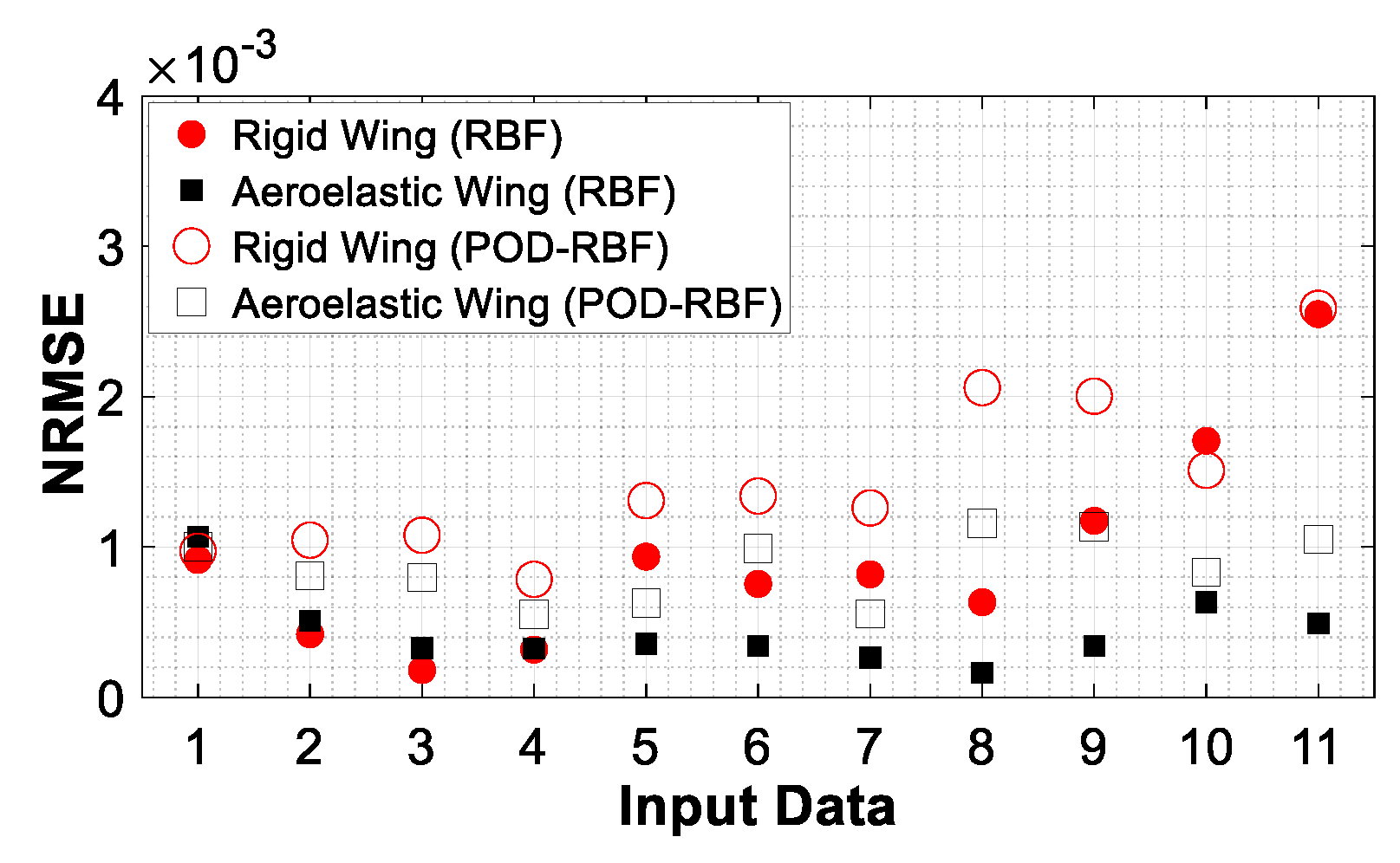
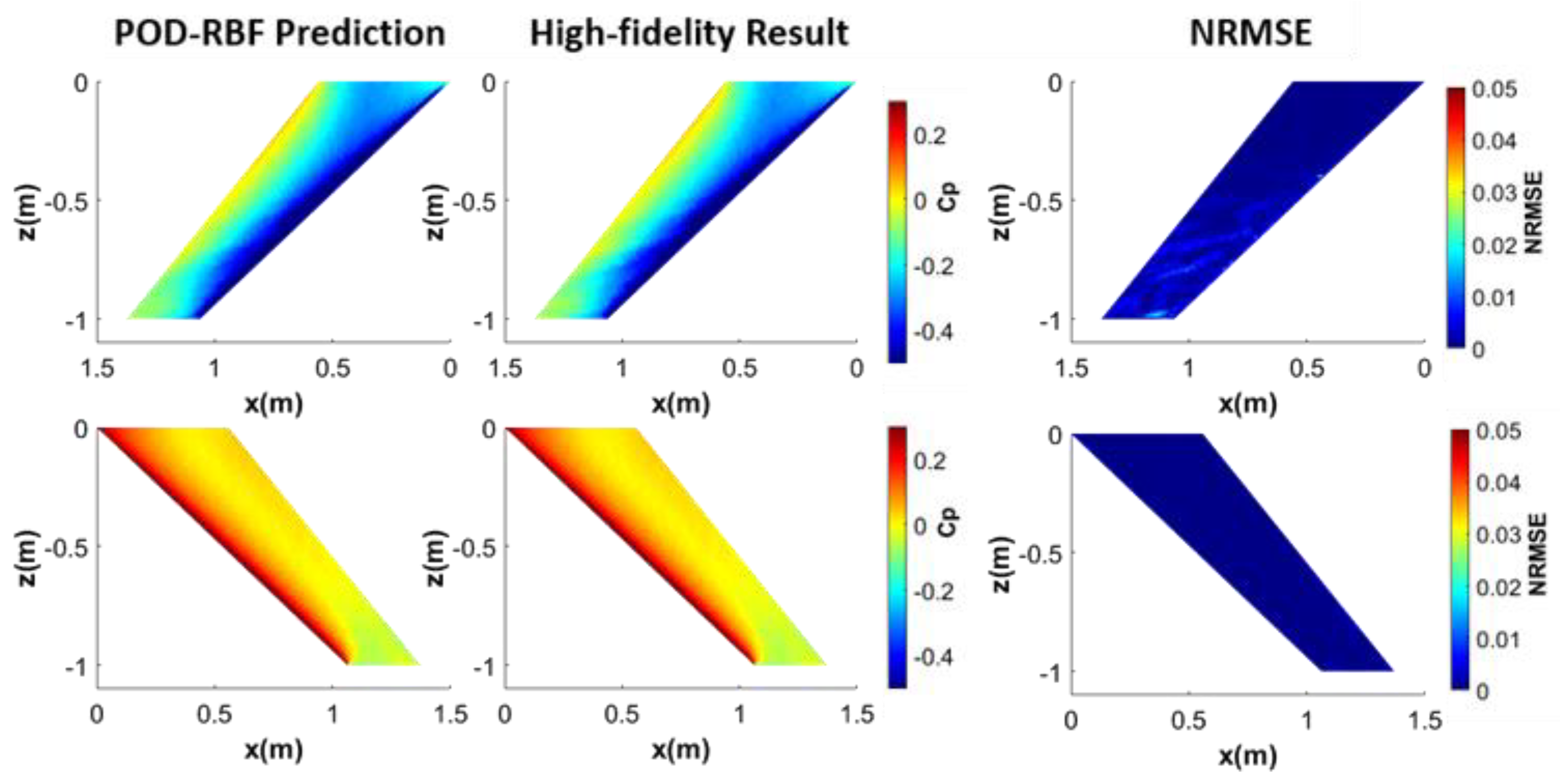
From the NRMSE results given for 10 randomly selected data points and the 11th data point manually added, it is seen that for both rigid and aeroelastic wings a significant accuracy is obtained for the Cp distribution, with NRMSE values less than 4 × 10⁻³. In accordance with the findings inferred from the reconstruction study, the accuracy of the aeroelastic wing is slightly higher than that of the rigid wing. For the Mach number and the AOA flow condition of M = 0.83 and AOA = 4.75°, corresponding to the highest Mach number and the AOA pair in the intermediate data set, the prediction performance is investigated in more detail for both rigid and aeroelastic wings. In the previous section, it was concluded that 8 modes out of 63 were required to capture 90% of the energy to provide sufficient accuracy in terms of flow reconstruction for the rigid wing. In this section, the POD coefficients corresponding to 8 POD modes are interpolated via the RBF method to obtain the POD coefficients. For this case, the POD coefficient matrix that is used for the regression analysis is 63 × 8. The resultant Cp distributions obtained by high-fidelity CFD analysis and the coupled POD–RBF method for M = 0.83 and AOA = 4.75° are displayed on the 3D rigid wing in Figure 15.

Figure 15 shows that predicted pressure distributions match the high-fidelity CFD results with great accuracy. The NRMSE plots show that the NRMSE is higher on the top surface of the rigid wing compared to the bottom surface, which is due to the higher distortion of the flow over the top surface compared to the bottom surface. To observe the differences more clearly, sectional results at 0.95, 0.55 and 0.15 span locations are given in Figure 16.

The Cp distribution at a spanwise section taken through the aerodynamic center of the wing, as shown in Figure 17a, is displayed in Figure 17b, where Cp values at the nodes located within a 0.0015 m interval from the selected spanwise section are used for this purpose.

From Figure 16 and Figure 17, one can see that the sectional Cp variations predicted by the POD-RBF method match well with the full order result. For the rigid wing, the R², RMSE and NRMSE for the POD-RBF prediction of the Cp at the flow condition M = 0.83 and M = 4.75° are calculated as 0.9996, 0.0058 and 0.0026, which shows the great accuracy of the POD-RBF prediction capability for the rigid wing.

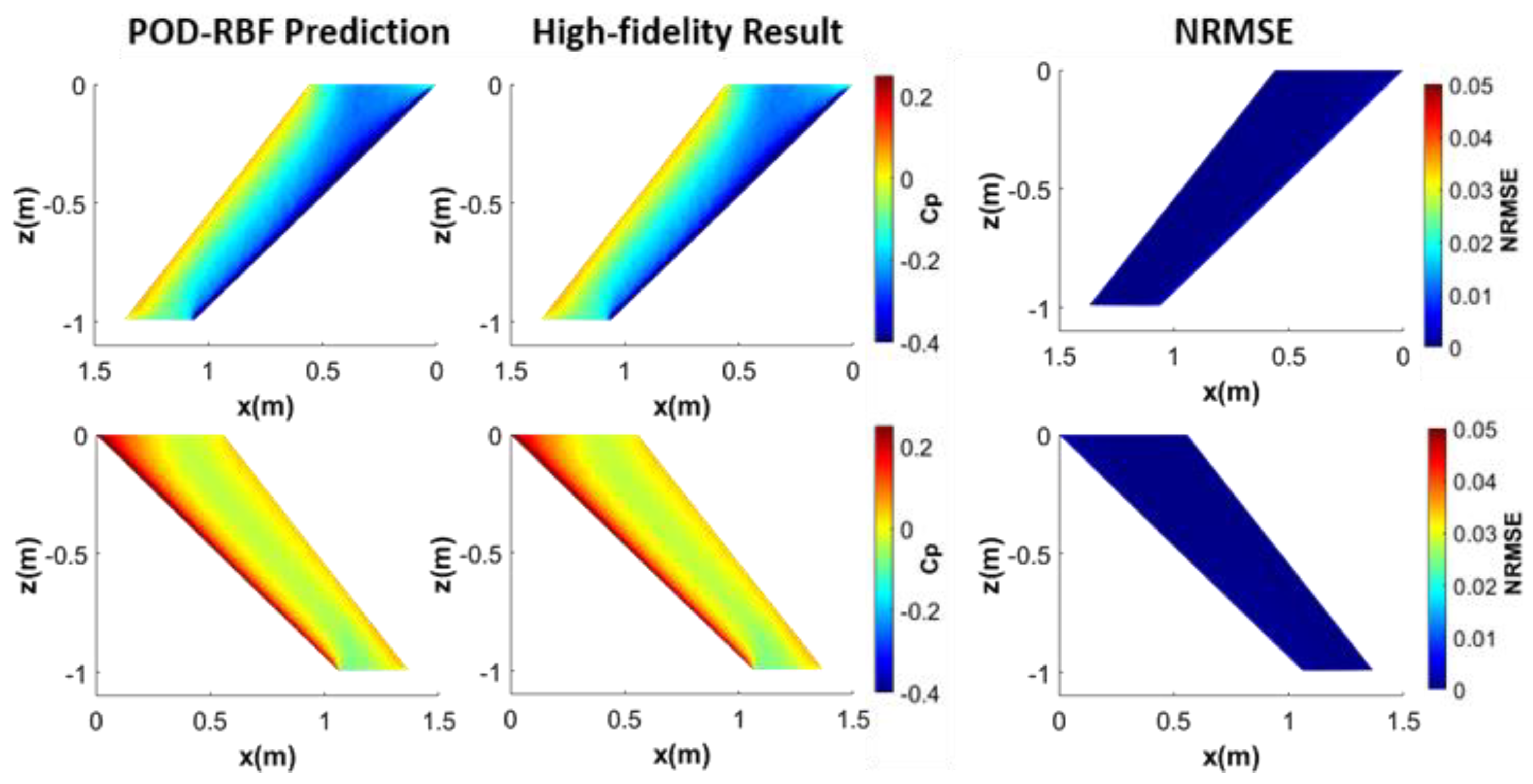
For the same flow condition (M = 0.83 and AOA = 4.75°), 5 modes out of 63 were required to capture 90% of the energy to provide sufficient accuracy in terms of Cp reconstruction for the aeroelastic wing. In this case, the POD coefficients corresponding to 5 POD modes are interpolated via the RBF method. Moreover, for the aeroelastic wing, while constructing the following Cp distribution plots, positions of the nodes were also taken into account, unlike the rigid wing case. It should be recalled that for the position of the nodes only 1 mode was required to obtain sufficient accuracy. Hence, by interpolating the POD coefficients corresponding to 1 mode, required POD coefficients for the M = 0.83 and AOA = 4.75° flow case are obtained. The resultant Cp distributions are displayed on the 3D wing in Figure 18.

Figure 18 clearly shows that predicted Cp distributions match perfectly with the Cp distributions obtained by high-fidelity static aeroelastic analysis. For the aeroelastic wing, the R², RMSE and NRMSE for the POD-RBF prediction of the Cp at the flow condition M = 0.83 and M = 4.75° are calculated as 0.9999, 0.0024 and 0.0011, respectively. It is noted that compared to the rigid wing case, even with 5 POD modes in the coupled POD-RBF ROM, a better prediction of the Cp distribution is achieved in the aeroelastic sweptback wing compared to the Cp predicted by the coupled POD-RBF ROM of the rigid wing with 8 POD modes. Moreover, the NRMSEs on the top and bottom surfaces of the aeroelastic wing are closer to each other compared to the rigid wing case. As displayed in Figure 13, because of the bending–twisting coupling effect of the sweptback wing geometry, the distortion of pressure distributions on the top and bottom surfaces of the aeroelastic wing is less compared to the rigid wing. Hence, NRMSE differences between the top and bottom surfaces are less compared to the rigid wing.

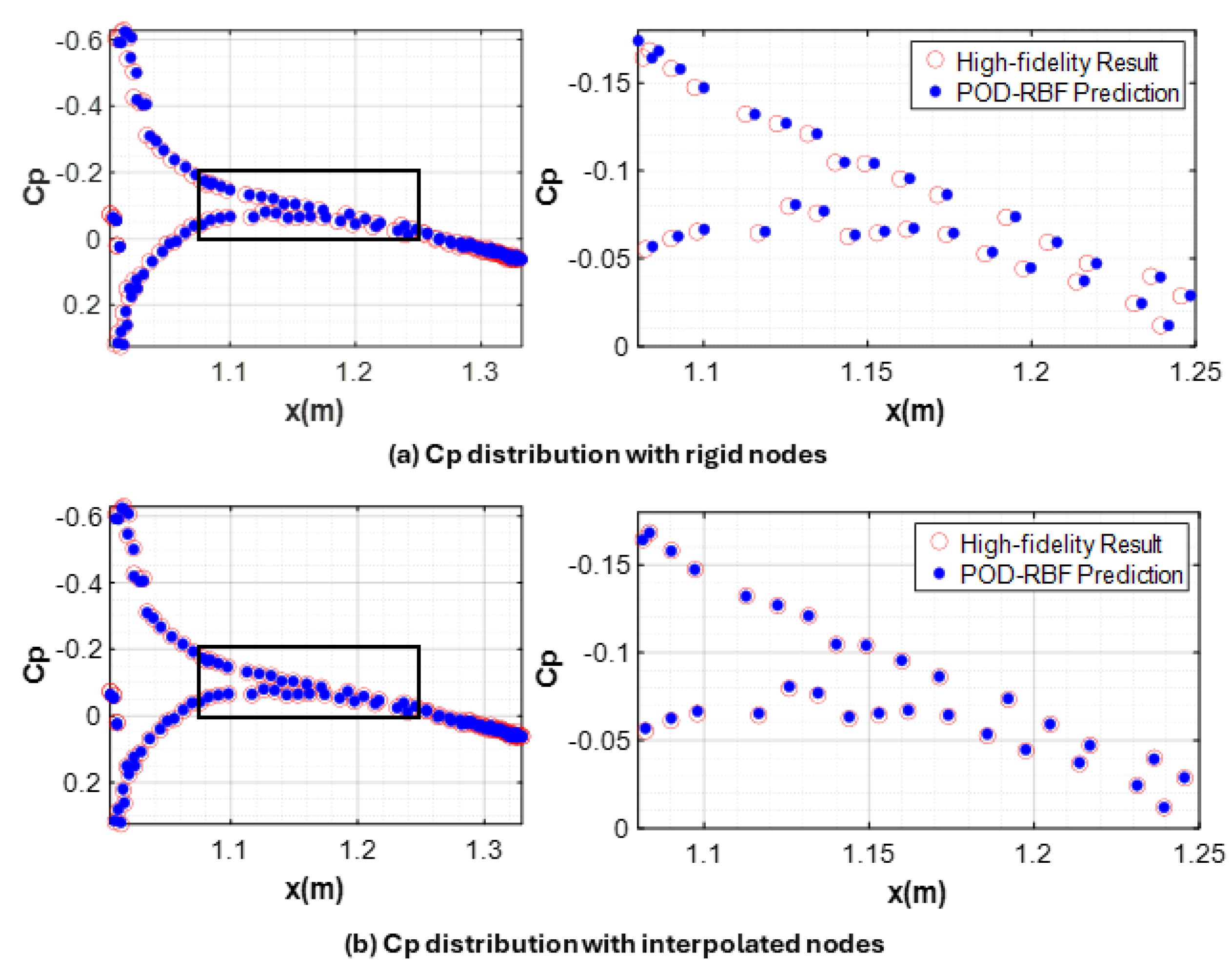
For the aeroelastic wing, Cp variations are also displayed along the chordwise and spanwise sections of the wing first, by keeping the nodes constant as in the case of rigid wing. Hence, no additional snapshot matrices are constructed for the position of the nodes and no ROM is constructed for the nodal positions. Then, positions of the nodes are also taken into account via a ROM with 1 mode to see the differences in Cp variations more clearly along the chordwise and spanwise sections. Figure 19 and Figure 20 show the chordwise and spanwise Cp variations, respectively. In Figure 19, chordwise variation of the Cp is shown at the 0.95 span location, and in Figure 20, the spanwise section along the aerodynamic center of the wing, shown in Figure 17, is taken to plot the spanwise variation of the Cp.

Zoomed views in Figure 19 and Figure 20 clearly show that there is an improvement in the predicted Cp results via the POD-RBF interpolation if the positions of the nodes are also taken into account by constructing a separate POD model and coupling it with the RBF method for interpolation. It should further be noted that for more flexible wings, the differences in Cp variation obtained by utilizing rigid nodes and interpolated nodes will be more pronounced; hence, a separate ROM for the positions of the nodes stands out as a necessity for flexible wings. As a by-product of utilizing a separate POD-RBF coupled ROM for the position of the nodes, it is also possible to calculate the displacement of the aeroelastic wing. For the M = 0.83 and AOA = 4.75° flow condition, while the maximum displacement is calculated as 0.1454 m by the full order analysis, utilizing the coupled POD-RBF ROM method maximum wing deflection is predicted very accurately as 0.147 m.

Moreover, for the aeroelastic wing, another reduced order model is constructed for von Mises stress distribution in the wing, utilizing the results from the 2-way static aeroelastic analysis. In this case, it is seen that 1 mode captures 96.5% of the energy. From the reduced order model constructed for the von Mises stress distribution, stress distribution at M = 0.83 and AOA = 4.75° is also calculated. The predicted von Mises stress distributions via the coupled POD-RBF method and von Mises stress distributions calculated by high-fidelity static aeroelastic analysis on the top and bottom wing surfaces are shown in Figure 21.

Figure 21 shows the well-matched results of the high-fidelity analysis and the POD-RBF predicted von Mises stress distributions with an R², RMSE and NRMSE of 0.9997, 0.0384 and 0.0043, respectively. Moreover, the maximum von Mises stresses obtained by the full order aeroelastic analysis is 8.88 MPa, whereas from the coupled POD-RBF approach it is found to be 8.94 MPa.

In order to predict the results at intermediate variables that do not exist in the original data ensemble, a surrogate model based on the RBF method can also be used; hence, the model is not reduced and a surrogate model is constructed directly using the original snapshot matrix. Ten random variables introduced in Figure 14 are used as intermediate parameters for prediction purposes. For both rigid and aeroelastic wings, NRMSE values of the Cp distribution for each intermediate variable, obtained using the coupled POD-RBF ROM and the RBF-based surrogate model, are shown in Figure 22.

As is the case for the POD-RBF ROM prediction, all NRMSE results are below 4 × 10⁻³ for both rigid and aeroelastic wings, showing the high accuracy of the RBF-based surrogate model for Cp distribution; however, for the majority of the results predictions for the aeroelastic wing give more accurate results. On the other hand, it is seen that for flow conditions with a very low Mach number, the accuracy of the results for both configurations is very similar. In addition, it is also seen that even though both methods give highly accurate results, accuracy of the prediction of the RBF-based surrogate model is slightly higher than that of the POD-RBF ROM. Since, in the RBF-based surrogate model, the RBF method is applied directly on the snapshot matrix, the slightly higher accuracy of the RBF-based surrogate model compared to the POD-RBF ROM is reasonable.

As in the case of the coupled POD-RBF ROM approach for the aeroelastic wing, a separate surrogate model is constructed utilizing the snapshot matrices of the positions of the nodes. Maximum deflections at the intermediate flow condition of M = 0.83 and AOA = 4.75° obtained from high-fidelity static aeroelastic analysis and the RBF surrogate model prediction are 0.1454 m and 0.1459 m, respectively, showing a great match. Moreover, from the snapshot data for the von Mises stress distribution, von Mises stress distribution at M = 0.83 and AOA = 4.75° is obtained via the surrogate model based on the RBF method. The maximum von Mises stresses as well as maximum deflections obtained from both methods are summarized in

Table 3. Maximum deflection and von Mises stress results for the POD-RBF and RBF ROMs (M = 0.83 and AOA = 4.75°).

	High-Fidelity	POD-RBF	RBF
Maximum Deflection (m)	0.1454	0.1470	0.1459
Maximum von Mises Stress (MPa)	8.88	8.94	8.95

.

Our results show that both the POD-based ROM coupled with the RBF method and the RBF-based surrogate model have almost the same accuracy, very close to the results of the high-fidelity analysis. In terms of computational time, a comparison of the methods is given in

Table 4. Comparison of the computational time for the Cp distribution for the rigid and the aeroelastic wing (M = 0.83 and AOA = 4.75°) *.

	High-Fidelity	POD-RBF	RBF
Rigid Wing	1366.5 s	3.2 s	3.6 s
Aeroelastic Wing	3251.2 s	10 s	13 s

* On an AMD Ryzen 7-5800X 8-Core Processor and 3.80 GHz computer.

.

As Table 4 shows, utilizing the POD-based ROM or the RBF-based surrogate model to predict the solutions for flow conditions that are not contained in the original data set saves a great amount of computational time. It should be noted that for the aeroelastic wing, interpolation of the nodal positions is also included in the computational time for both the POD-RBF-based ROM and the RBF-based surrogate modeling; therefore, its computational time is higher than for the rigid wing.

Here it should also be noted that, in the current case, in order to construct a snapshot matrix, high-fidelity analyses are run for 63 flow conditions, which requires a great computational cost. In addition, to decide on the number of POD modes in order to capture the features of the data domain effectively, the reconstructed results are compared with the actual ones, and this process takes time during the construction of the POD-based ROM. Moreover, to find an appropriate basis function and shape parameter for the RBF, the models are run several times. However, since obtaining a result takes a few seconds with the ROM or the surrogate model, compared with the computational cost of the construction of a snapshot matrix, the computational cost of the training process is negligible. In the present study, static aeroelastic analyses of the sweptback wing took approximately 57 h to complete in order to create a snapshot matrix. Hence, for an individual static aeroelastic analysis or rigid CFD analysis for a given flow condition, performing a high-fidelity analysis should be preferred instead of constructing a ROM or a surrogate model. However, for complex and higher order problems involving repeated analysis, such as optimization, uncertainty quantification, etc., constructing a ROM or a surrogate model is usually justified, and for these cases the computational cost of constructing a ROM or a surrogate model is worthwhile.

In this study, it is concluded that both the coupled POD-RBF ROM and RBF-based surrogate modeling have almost the same level of accuracy; however, there is a difference in terms of computational time such that the RBF-based surrogate model has a slightly higher computational cost than the POD-RBF-based reduced order model. This is because the RBF-based surrogate model includes the RBF interpolation of the whole data set; whereas, for the POD-based ROM, RBF interpolation is applied only to the POD coefficient matrix whose data size is far less than the snapshot matrix. Moreover, since the aeroelastic wing includes the effect of nodal positions, the difference in the computational time becomes more explicit in favor of the POD-RBF-based ROM. For a crowded analysis model with a higher number of data points and nodes, the difference in computational time would increase substantially, with an inevitable increase in memory demand.

It should be noted that constructing the surrogate model consists of only the application of the RBF method on the snapshot data, while constructing the coupled POD-RBF reduced order model includes the whole process of the POD method, which includes the application of the MOS technique on the modified snapshot matrix to find the basis vectors and deciding on the significant number of modes, calculating the POD coefficients by multiplying the basis vectors with the data in hand and applying the RBF method to these POD coefficients. Afterwards, basis vectors are multiplied by the POD coefficients calculated utilizing the RBF method, and the mean of the snapshot data is added to reach the desired result. Hence, compared to the coupled POD-RBF ROM, the RBF-based surrogate model can be considered as more practical in its application.

5. Conclusions

In this study, the effect of wing elasticity on the efficiency of the POD-based ROM method is presented by implementing the method with respect to both rigid and aeroelastic sweptback wings for different flow conditions. In the literature, there are several studies on reduced order modeling applications for the investigation of the aeroelastic and rigid aerodynamic behavior of aerospace structures utilizing POD-based ROMs. However, the effect of bending–twisting coupling in aeroelastic sweptback wing configurations on the more effective application of POD-based ROMs, compared to rigid sweptback wing configurations, has not been studied before. To the best of our knowledge, such a study does not exist in the literature, and this is a novel feature of our study. We believe that for flexible sweptback wings of future high aspect ratio aircraft designs, the findings of the present study will prove to be a benchmark for the ROM community.

The present study shows that reduced order modeling is more effectively applied to the aeroelastic wing when the pressure coefficient (Cp) is taken as the output; this is because for the elongated AGARD 445.6 wing configuration studied, to reach 90% of the captured energy of the modes, 8 POD modes are required for the rigid wing, whereas 5 POD modes are sufficient for the aeroelastic wing. The main reason for this is attributed to the bending–torsion coupling mechanism which occurs in sweptback wing geometries. Since bending–torsion coupling accounts for reducing the effective angle of attack of the aeroelastic wing configuration, it is concluded that because of the separation of flow around the rigid wing at a lower angle of attack compared to the aeroelastic wing, the Cp distribution pattern is disrupted; hence, a higher number of modes is required to reach 90% of the energy. There is no drastic change in the Cp distribution pattern for the aeroelastic wing compared with the rigid wing, and this results in more effective reduced order modeling for the aeroelastic wing.

In addition, for the aeroelastic wing, the location of the nodes changes due to deflection of the wing; therefore, contrary to the rigid wing, each case analyzed has its own node positions. In this case, it is shown that separate snapshot matrices for the x, y and z positions of the nodes have to be constructed, and the POD-based ROM has to be applied also for the positions of the nodes in order to obtain Cp distributions slightly more accurately for the current wing configuration. However, for more flexible wing configurations with higher wing deflections, the deformed positions of the nodes will be highly influential on the accurate display of the Cp distribution. It is concluded that for flexible wings, utilizing rigid nodes is not sufficient for presenting the Cp distribution accurately; hence, separate ROMs must be generated for the deformed x, y and z positions of the nodes. Moreover, as a by-product of separate ROMs generated for the positions of the nodes, a deflection prediction of the wing is also made. Similarly, von Mises stress distribution for the aeroelastic wing can be reconstructed very accurately via the same process with a significant reduction of order.

The prediction capability of the POD-based ROM is also demonstrated by coupling it with the RBF-based regression method. For this purpose, predictions of aerodynamic (Cp) and structural metrics (deflection and stress) are performed at 11 intermediate data points that do not exist in the original data set. It is shown that accurate prediction of both aerodynamic and structural metrics can be made for the flow conditions that do not exist in the original data set using the coupled POD-RBF ROM. It is shown that compared to the rigid wing case, even with 5 POD modes in the coupled POD-RBF ROM a slightly more accurate prediction of the Cp distribution is achieved in the aeroelastic wing compared to the Cp predicted by the coupled POD-RBF ROM of the rigid wing with 8 POD modes. The main reason for this is attributed to the bending–torsion coupling of the sweptback wing geometry causing a reduction in the effective angle of attack, thereby reducing the distortion of the flow mainly on the top surface of the wing, hence increasing the prediction capability of the coupled POD-RBF ROM.

In addition to the POD-based ROM coupled with the RBF method, surrogate models based on the RBF method are constructed for the prediction of results with direct interpolation of the data ensemble in a comparative manner. It is seen that both the POD-based ROM coupled with the RBF method and the RBF-based surrogate models have almost the same level of accuracy; they both produce results which are very close to the results of the high-fidelity analyses. Furthermore, both methods save a great amount of computational time compared to the high-fidelity analysis. However, the RBF-based surrogate model has a higher computational cost than the POD-RBF-based reduced order model since the RBF-based surrogate model includes the RBF interpolation of the whole data set; whereas, for the POD-based ROM, RBF interpolation is applied only to the POD coefficient matrix whose data size is far less than the snapshot matrix. On the other hand, for less crowded analysis models with a smaller sized snapshot matrix, then constructing the RBF-based surrogate model and utilizing it for predicting results at intermediate data points which are not in the original snapshot matrix is more practical since the computational process is simpler.