New Data-Driven Models of Mass Flow Rate and Isentropic Efficiency of Dynamic Compressors

Abstract

Dynamic compressors are widely used in many industrial sectors, such as air, land, and marine vehicle engines, aircraft environmental control systems (ECS), air-conditioning and refrigeration, gas turbines, gas compression and injection, etc. The data-driven formulas of mass flow rate and isentropic efficiency of dynamic compressors are required for the design, energy analysis, performance simulation, and control- and/or diagnosis-oriented dynamic simulation of such compressors and the related systems. This work develops data-driven models for predicting the performance of dynamic compressors, including empirical models for mass flow rate and isentropic efficiency, which have high prediction accuracy and broad application range. The performance maps of two multi-stage axial compressors of an aero engine and a centrifugal compressor of an aircraft ECS were chosen for evaluation of the existing empirical formulas and testing of the new models. There are 16 empirical models of mass flow rate and 14 empirical models of isentropic efficiency evaluated, and the results show that it is necessary to develop highly accurate empirical formulas both for mass flow rate and isentropic efficiency. With the data-driven method, two empirical models for mass flow rate and one for isentropic efficiency are developed. They are in general form, with some terms removable to make them simple while enhancing their applicability and prediction accuracy. The new models have much higher prediction accuracy than the best existing counterparts. The new mass flow rate models predict for the three compressors a mean absolute relative deviation (MAD) not greater than 1.3%, while the best existing models all have MAD > 2.0%. The new efficiency model predicts for the three compressors an MAD of 1.0%, 0.4%, and 1.9%, respectively, while the best existing model predicts for the three compressors an MAD of 1.8%, 0.8%, and 3.2%, respectively.

1. Introduction

Dynamic compressors are widely used in many industrial sectors, such as air, land, and marine vehicle engines, aircraft environmental control systems (ECSs), air-conditioning and refrigeration, gas turbines, turbochargers, gas compression and injection, air compression for producing compressed air, pipeline compression for gas transport, electric power generation applications for industrial power plants, and combined heat and power systems for buildings, and they are also used in oil refineries, chemical and petro-chemical plants, and natural gas processing plants [1,2,3,4,5].

The mathematical models of isentropic efficiency (also called efficiency or adiabatic efficiency) and mass flow rate of compressors are necessary for performance study, energy analysis, and control- and/or diagnosis-oriented dynamic simulation of systems including compressors. These models may be built by a mechanism analysis method, a data-based method, or a hybrid method.

The mechanism analysis method is based on theoretical analysis and studies the intrinsic mechanism of the physical object, building a mathematical model from the physical laws of mass, energy and momentum conservation. The obtained model is called the mechanism model. Dynamic compressors are thermal fluid components, for which the mechanism analysis method is generally based on the conservation laws of mass, energy, and momentum in thermal fluid mechanics, yielding a model usually with some form of the Navier–Stokes equation. Solving this kind of mechanism models involves complex numerical operations, such as the computational fluid mechanics (CFD) manipulation [6,7,8], which is so computationally intensive and inefficient that it is unfit for control- and/or diagnosis-oriented dynamic simulation and less attractive than data-driven counterparts.

The data-based method may be classified into the data-driven, the graphical, and the tabular methods. The graphical method usually models compressors using performance maps, and the tabular method uses look-up tables. Due to the difficulty of data-driven modeling for dynamic compressors, the graphical and tabular methods were widely used in early modeling and simulation [9,10], and are still frequently used today [11,12]. Yang et al. [11] used the Ansys CFX software to obtain turbine and compressor performance maps for the performance simulation and analysis of a reversed bootstrap ECS. Jennings et al. [12] used performance maps to calculate the performance of the compressor and turbine in the modeling and simulation of the B737-800 passenger aircraft ECS.

Data-driven methods are based on available data, discovering correlations and mathematical relationships between the variables among the data, and then expressing these relationships mainly in the form of a mathematical formula or artificial neural network. The former is often referred to as an empirical formula, empirical model, or correlation. An empirical formula is also called a mean value model in some literature regarding turbochargers and land vehicle engines [13,14,15].

The main categories of the data-driven methods include the regression analysis method, the artificial intelligence method, and the curve fitting method [16,17,18]. The regression analysis method includes linear regression, nonlinear regression, and Gaussian process regression, etc. The artificial intelligence method includes artificial neural networks (ANN), machine learning, and genetic algorithms, etc. In the actual modeling process, these methods are often used interchangeably. For example, Zhang and Duraisamy [17] used multi-scale Gaussian process regression and neural network methods in machine learning based modeling. In addition, different literature may have inconsistent definitions or different names for a certain method. For example, Ahmad et al. [18] use the terms of the regression analysis method and the statistical modeling method alternately.

Among data-driven modeling methods, the regression analysis is the most widely used, and can be used alone or in combination with other methods. Using the regression analysis method, Pulpeiro Gonzalez and Hall [19] obtained the empirical formulas representing the mass flow rate and isentropic efficiency maps of turbine and compressor. Using the non-parametric regression method, Sun et al. [20] obtained the health indices for ECS health management based on the ECS flight parameters detected onboard. Regression analysis methods are often used in conjunction with other methods. For example, Fang et al. [21,22] first used the Taylor expansion method to obtain the basic model for the mass flow rate and isentropic efficiency of cooling turbines, and then determined the number of terms and constants using regression analysis methods based on experimental data.

In the artificial intelligence method, ANN and machine learning methods are most commonly used, and machine learning methods are often aided by other methods, such as ANN and regression analysis. Nikiforov et al. [23] established a mathematical model using an ANN method to replace the performance maps of a centrifugal compressor. Fei et al. [24] proposed an artificial intelligence method combining the feedforward backpropagation neural network and the Gaussian kernel function to predict the performance maps of a multi-stage axial compressor and compared it with the feedforward backpropagation neural network method and the support vector machine method. Zhang and Duraisamy [17] attempted to add terms to the turbulent Reynolds averaged equation to improve its accuracy and applicability. The added items were obtained using a machine learning method called supervised learning. Uzun et al. [25] used a deep machine learning method and an ANN method to establish an aircraft fuel consumption model based on the given meteorological and flight data.

The least squares method is commonly used in curve fitting methods. Tu and Chen [26] used it to obtain the mass flow rate and isentropic efficiency formulas based on a compressor performance map for a MAN Diesel & Turbo TCA88 turbocharger from Augsburg, Germany. Li et al. [27] used a partial least squares curve fitting method to obtain the mass flow rate and isentropic efficiency formulas for a variable geometry compressor in a diesel engine.

The hybrid modelling method is the combination of the mechanism analysis method and the data-driven method. It utilizes the mechanism analysis method to establish a basic mathematical model of the system through appropriate simplification and uses the data-driven method to determine the constants and terms in the model, and the resultant model is also known as a semi-empirical formula, or simply called an empirical formula. Due to the use of the data-driven method in the modeling process, the hybrid method is also categorized as a data-driven method in some literature. Using the hybrid modelling method, Yang and Yang [28] established an equation for the number of transfer units (NTU) in ECS heat exchangers, with the heat transfer coefficient in the NTU equation determined based on experimental data. Chen et al. [29] obtained the basic performance models of a centrifugal compressor through theoretical analysis, with the constants in the models to be determined using the genetic algorithm based on experimental data.

In the above data-driven modelling methods, regression analysis, curve fitting, and hybrid methods yield empirical formulas, which are the dominant models for dynamic compressors because they are compact and time-efficient in design, analysis and performance simulation and favorite for control- and/or diagnose-oriented dynamic simulation among such compressors and systems [30,31].

There are a number of empirical formulas for compressor mass flow rate and isentropic efficiency for turbochargers and land and marine vehicle engines [13,14,15,26,30,32,33,34,35,36,37,38,39,40,41]. However, for dynamic compressors used in aero engines and aircraft ECSs, the empirical formulas of the mass flow rate and isentropic efficiency are rare, with only two papers [42,43] found presenting the empirical formulas for aero engine compressors and two articles [44,45] found for the empirical formulas for aircraft ECS compressors. In addition, our systematic review and evaluation show that the prediction accuracy of the existing empirical models for mass flow rate and isentropic efficiency is not satisfactory for the dynamic compressors of aero engines and aircraft ECSs, and thus new models with a high accuracy need to be developed [1,31,44,45].

The purpose of the present paper is to meet the above needs, developing the empirical formulas of mass flow rate and isentropic efficiency that have high prediction accuracy and broad application range for dynamic compressors, with an emphasis on their application to aero engines and aircraft ECSs. For this purpose, the empirical models of mass flow rate and isentropic efficiency for existing dynamic compressors are reviewed, and the reviewed models are evaluated with the performance data of aero engine and aircraft ECS compressors. Then, new empirical formulas for the mass flow rate and isentropic efficiency of dynamic compressors are developed using data-driven methods. Considering that most of the existing models have fixed terms, which may be accurate for the authors’ own data, but usually experience large deviation when applied to data from other sources, the new models are in general form, with some terms removable to simplify them while enhancing their applicability and prediction accuracy. Several data-driven methods are tested to select one which produces the best result.

2. Existing Empirical Models of Compressor Mass Flow Rate and Isentropic Efficiency

2.1. Basic Parameters of Dynamic Compressors

• Parameters regarding mass flow rate

For a dynamic compressor, the mass flow rate G may be indirectly expressed as the normalized mass flow rate parameter ϕ and the corrected mass flow rate ϕ_corr.

$$\varphi ={\displaystyle \frac{G}{\frac{\pi }{4}{d}^{2}U{\rho }_{in}}}$$

(1)

$${\varphi }_{corr}=G\left({\displaystyle \frac{p_{ref}}{p_{in}}}\right)\sqrt{{\displaystyle \frac{T_{in}}{T_{ref}}}}$$

(2)

where G is the mass flow rate; d is the blade wheel diameter; U is the blade tip speed; ρ, p and T are the air density, pressure, and temperature, respectively; and the subscripts in and ref denote the inlet and reference point, respectively. The reference point is usually set at T = 288.15 K and p = 101,325 Pa. The compressor tip speed U is defined as

$$U=\pi dn$$

(3)

where n is the compressor rotational speed. Other useful parameters regarding the compressor rotational speed are the rotational speed parameter n_t, the corrected rotational speed n_corr, and the rotational speed ratio n_r, as defined below:

$$n_t={\displaystyle \frac{n}{\sqrt{T_{in}}}}$$

(4)

$$n_{corr}=n\sqrt{{\displaystyle \frac{T_{ref}}{T_{in}}}}$$

(5)

$$n_r=n/n_{ref}$$

(6)

where n_ref is the compressor rotational speed at the reference point, usually the design point.

Some researchers [13,14] have related the mass flow rate to the dimensionless head parameter ψ, which is defined as

$$\psi ={\displaystyle \frac{c_p{T}_{in}({{\pi }_c}^{\frac{k-1}{k}}-1)}{\frac{1}{2}{U}^2}}$$

(7)

where c_p is the gas specific heat at constant pressure, k is the isentropic exponent, and π_c is the compressor compression ratio.

$${\pi }_c={\displaystyle \frac{p_{out}}{p_{in}}}$$

(8)

Some researchers [39,43] correlate the mass flow rate indirectly by setting the compression ratio as the function instead of the mass flow rate.

2.

Compressor isentropic efficiency

The compressor isentropic efficiency η (sometimes called adiabatic efficiency, or simply efficiency) is defined as

$$\eta ={\displaystyle \frac{W_s}{W}}$$

(9)

where W_s and W are the compressor isentropic compression work and actual compression work, respectively.

$$W_s=G{c}_p{T}_{in}\left({{\pi }_c}^{\frac{k-1}{k}}-1\right)$$

(10)

$$W=G{c}_p\left(T_{out}-T_{in}\right)$$

(11)

Substituting Equations (10) and (11) into Equation (9) yields

$$\eta =\left({{\pi }_c}^{\frac{k-1}{k}}-1\right)/\left({\displaystyle \frac{T_{out}}{T_{in}}}-1\right)$$

(12)

2.2. Existing Empirical Formulas for Compressor Mass Flow Rate

The available existing empirical formulas for compressor mass flow rate are listed in

Table 1. Existing empirical models for compressor mass flow rate.

Sources	Models	Remarks
Jensen et al. [13]	$\psi =\frac{A_1+A_2\varphi }{A_3-\varphi }$ $A_i=a_{i1}+a_{i2}Ma,\begin{array}{ccc} & & i=1,2,3\end{array}$ where coefficients aij are determined through the least square fit on experimental data, and the Mach number Ma is defined as $Ma=\frac{U}{\sqrt{{kRT}_{in}}}$ where R is the gas constant.	They proposed the model when studying the compressor of a 1.6 L turbocharged indirect injection diesel engine.
Mueller [14]	$\psi =A_1+A_2\varphi +A_3{\varphi }^2$ $A_1=a_1+a_{2}U+a_3{U}^2$ $A_2={\displaystyle \frac{-2A_3{G}_{top}}{U}}$ $G_{top}=a_4+a_{5}U+a_6{U}^2$ $A_3=a_7+a_{8}U+a_9{U}^2$	Mueller proposed the polynomial model to simulate the compressor of turbocharged spark ignition (SI) engines.
Tu and Chen [26]	${\varphi }_c=a+\left(1-e^{{\psi }^c+b}\right)$ where the coefficients a, b, c are fitted by polynomial function of the Mach number Ma as in the following: $a=a_{m}M{a}^m+a_{m-1}M{a}^{m-1}+\dots +a_{1}Ma+a_0$ $b=b_{n}M{a}^n+b_{n-1}M{a}^{n-1}+\dots +b_{1}Ma+b_0$ $c=c_{l}M{a}^l+c_{l-1}M{a}^{l-1}+\dots +c_{1}Ma+c_0$ where the order of the polynomials m, n, l are obtained from the actual curve fitting.	They proposed the exponential model and implemented a case study of a compressor map for the TCA88 turbocharger to verify it.
Andersson [32]	$\varphi =a_1\sqrt{1-a_2{\psi }^2}$ where $1-a_2{\psi }^2\ge 1$.	Andersson reasoned that the normalized mass flow rate could be described using only the head parameter and thus proposed a model for the compressor of turbocharged SI engines.
Kolmanovsky et al. [33,34]	${\displaystyle \frac{\varphi }{{\varphi }_{top}}=}\left\{\begin{array}{c}1+\beta \left\{1-\exp \left[a_5\left({\displaystyle \frac{{\pi }_c}{{\pi }_{c,top}}}-1\right)\right]\right\}\begin{array}{cc}& \mathrm{for}{\pi }_c<{\pi }_{c,top}\end{array}\hfill \\ 1-\beta a_5\left({\displaystyle \frac{{\pi }_c}{{\pi }_{c,top}}}-1\right)\begin{array}{ccc}& & \mathrm{for}{\pi }_c>{\pi }_{c,top}\end{array}\hfill \end{array}\right.$ ${\varphi }_{top}=a_1{n}_t+a_2{n}_t^2$ ${\pi }_{c,top}=a_3+a_4{\varphi }_{top}^2$ $\beta =a_{6}exp(-a_7{n}_t)$ where ϕtop is the maximum normalized mass flow rate on each speedline, and πc,top is the compression ratio corresponding to ϕc,top.	They proposed the model for compressors used in automobile turbocharged diesel engines.
Tsoutsanis et al. [35,36]	${\displaystyle \frac{{\varphi }_{corr0}^2}{{a_{{\pi }_c}}^2}}+{\displaystyle \frac{{\pi }_{c0}^2}{{b_{{\pi }_c}}^2}}=1$ where $a_{{\pi }_c}$ and $b_{{\pi }_c}$ denote the semi-major and the semi-minor axes of the ellipse, respectively, and ϕcorr0 and πc0 denote the corrected mass flow rate and the compression ratio when the ellipse center is fixed at (0, 0).      Taking into consideration that each ellipse is free to rotate at an angle θ, then the ellipse’s new coordinates (ϕcorr, πc) are given by ${\varphi }_{corr}={\varphi }_{corr0}cos\left({\theta }_{{\pi }_c}\right)-{\pi }_{c0}sin\left({\theta }_{{\pi }_c}\right)$ ${\pi }_c={\varphi }_{corr0}sin\left({\theta }_{{\pi }_c}\right)+{\pi }_{c0}cos\left({\theta }_{{\pi }_c}\right)$ The coefficients $a_{{\pi }_c}$ and $b_{{\pi }_c}$ are expressed as $a_{{\pi }_c}=a_{{\pi }_{c1}}{n_{corr}}^3+a_{{\pi }_{c2}}{n_{corr}}^2+a_{{\pi }_{c3}}{n}_{corr}+a_{{\pi }_{c4}}$ $b_{{\pi }_c}=b_{{\pi }_{c1}}{n_{corr}}^4+b_{{\pi }_{c2}}{n_{corr}}^3+b_{{\pi }_{c3}}{n_{corr}}^2+b_{{\pi }_{c4}}{n}_{corr}+b_{{\pi }_{c5}}$	They proposed a compressor map tuning method to improve the accuracy and fidelity of gas turbine engine performance models. Axial compressor performance maps were used in their study.
Biteus [37]	$G=a_1\left(1-{\displaystyle \frac{1}{{\pi }_c}}\right)+a_{2}n{\left(1-{\displaystyle \frac{1}{{\pi }_c}}\right)}^{1/2}+a_{3}n{\left(1-{\displaystyle \frac{1}{{\pi }_c}}\right)}^{1/4}+a_{4}n$	The model was proposed for heavy duty diesel engine compressors.
Eriksson et al. [38]	$G=a_{1}P+a_2{P}^2+a_3{P}^3$ $P={\pi }_c+a_4{n}^{\prime }+a_5{n}^{\prime 2}$ where $n^{\prime }=5\times {10}^{-5}(n-8\times {10}^4)$.	They developed the model for turbocharged SI engine compressors.
Guzzella and Amstutz [39]	${\pi }_c=A_1+A_2{({\varphi }_{corr}-A_3)}^2$ where Ai (i = 1, 2, 3) depend on the shaft speed n only, and can be parameterized as polynomial functions.	They proposed the compressor model in studying the model-based control of diesel engines.
Jiang et al. [40]	${\pi }_c^{*}={\pi }_c^{(k-1)/k}$ ${\pi }_c^{*}=a_0+a_1{\varphi }_{corr}{n}_t+a_2{\varphi }_{corr}^2+a_3{\varphi }_{corr}^2{n}_t+a_4{n}_t^2+a_5\left({\displaystyle \frac{n_t^3}{{\varphi }_{corr}}}\right)$	The model was proposed for centrifugal compressors.
Orkisz and Stawarz [42]	$\varphi =a_0+a_1{n}_t+a_2{n}_t^2+a_3{n}_{t}Z+a_{4}Z+a_5{Z}^2$ where Z is the coefficient of relative stability margin of the compressor.	They rescaled a traditional axial compressor performance map in a coordinate system of (nt, Z, ϕ), based on which they proposed their model.
Sieros et al. [43]	1. Non-linear model, which can be reduced to ${\pi }_c=a_0+a_1{n}_r+{\displaystyle \frac{a_2+a_3{n}_r+a_4{n_r}^2}{a_5+G+a_6{n}_r}}$ 2. Simple linear model, which can be reduced to $G+{\pi }_c=a_1+a_2{n}_r{\left(G-{\pi }_c\right)}^2$ 3. Generalized linear model 1  The simplest form of the generalized linear models is $Y=A_1+A_{2}X$ $Y=G+{\pi }_c$ $X=n_r{\left(G-{\pi }_c\right)}^2$ $A_1=a_1+a_2{n}_r$ $A_2=a_3+a_4{n}_r$ 4. Generalized linear model 2  A further increase in accuracy may be achieved by using the following second-degree polynomial form: ${\pi }_c=a_1+A_{1}X+A_2{X}^2$ $X=n_r{({\pi }_c+G)}^2$ $A_1=a_2+a_3{n}_r+a_4{n}_r^2$ $A_2=a_5+a_6{n}_r$	They proposed four types of mass flow models for jet engine compressors: Non-linear model, simple linear model, generalized linear model 1, and generalized linear model 2. All of them incorporate the rotational speed ratio nr. The simple linear model, generalized linear model 1, and generalized linear model 2 are implicit, which are not convenient for use. since iteration is needed during the calculations.
Tian [44]	${\pi }_c={\displaystyle \frac{a_0+a_{1}ln{n}_r+a_2{\left(ln{n}_r\right)}^2+a_3\varphi +a_4{\varphi }^2}{1+a_{5}ln{n}_r+a_6\varphi }}$	The model was proposed to fit the performance map of an ECS compressor.

.

2.3. Existing Empirical Formulas for Compressor Efficiency

The available existing empirical formulas for compressor efficiency are listed in

Table 2. Existing empirical models for compressor efficiency.

Sources	Models	Remarks
Jensen et al. [13]	$\eta =a_1{\varphi }^2+a_2\varphi +a_3$ $a_i={\displaystyle \frac{a_{i1}+a_{i2}Ma}{a_{i3}-Ma}},\begin{array}{ccc} & & i=1,2,3\end{array}$	They proposed the model when studying the compressor of a 1.6 L turbocharged indirect injection diesel engine.
Canova et al. [15]	$\eta ={\displaystyle \frac{G{c}_p{T}_{in}\left({{\pi }_c}^{\frac{k-1}{k}}-1\right)\left(\frac{p_{ref}}{p_{in}}\right)\sqrt{\frac{T_{ref}}{T_{in}}}}{W_{corr}}}$ where Wcorr is difined as $W_{corr}=W\left({\displaystyle \frac{p_{ref}}{p_{in}}}\right)\sqrt{{\displaystyle \frac{T_{ref}}{T_{in}}}}$ and it is obtained by $W_{corr}=A_1+A_2{\varphi }_{corr}+A_3{{\varphi }_{corr}}^2+A_4{{\varphi }_{corr}}^3$ where the coefficients Ai (i = 1, 2, 3, 4) are linear functions of the corrected speed ncorr and can be obtained by fitting the compressor maps.	They proposed the model for automotive diesel engine compressors, where the corrected compression work Wcorr is treated as the function of the corrected mass flow rate ϕcorr.
Tu and Chen [26]	$\begin{array}{cc}\hfill \eta =& a_0+a_{1}Q+a_2{\pi }_c+a_3{Q}^2+a_{4}Q{\pi }_c+a_5{{\pi }_c}^2\hfill \\ \hfill & +a_6{Q}^3+a_7{Q}^2{\pi }_c+a_{8}Q{{\pi }_c}^2+a_9{{\pi }_c}^3+a_{10}{Q}^4\hfill \\ \hfill & +a_{11}{Q}^3{\pi }_c+a_{12}{Q}^2{{\pi }_c}^2+a_{13}Q{{\pi }_c}^3+a_{14}{{\pi }_c}^4\hfill \end{array}$ where Q is the volume flow rate.	They proposed the polynomial model and implemented a case study of a compressor map for the TCA88 turbocharger to verify it.
Andersson [32]	$\eta ={\eta }_{max}-{\chi }^{T}Q\chi$ ${\chi }^T=\left[{\varphi }_{corr}-{\varphi }_{corr,{\eta }_{max}},\left(1+\sqrt{{\pi }_c-1}\right)-{\pi }_{c,{\eta }_{max}}\right]$ $Q=\left[\begin{array}{cc}{a}_{11}& a_{12}\\ a_{12}& a_{22}\end{array}\right]$	Andersson proposed the model for the compressor of turbocharged SI engines by modifying the Guzzella and Amstutz model [39] with πc replaced by 1 + (πc − 1)0.5.
Tsoutsanis et al. [35,36]	${\displaystyle \frac{{\varphi }_{corr0}^2}{{a_{\eta }}^2}}+{\displaystyle \frac{{\eta }_0^2}{{b_{\eta }}^2}}=1$ where $a_{\eta }$ and $b_{\eta }$ denote the semi-major and the semi-minor axes of the ellipse, respectively, and ϕcorr0 and η0 denote the corrected mass flow rate and the efficiency when the ellipse center is fixed at (0, 0). The coefficients $a_{\eta }$ and $b_{\eta }$ are expressed as $a_{\eta }=a_{{\eta }_1}{n_{corr}}^2+a_{{\eta }_2}{n}_{corr}+a_{{\eta }_3}$ $b_{\eta }=b_{{\eta }_1}{n_{corr}}^3+b_{{\eta }_c}{n_{corr}}^2+b_{{\eta }_3}{n}_{corr}+b_{{\eta }_4}$ Taking into consideration that each ellipse is free to rotate at an angle θ, then the compressor isentropic efficiency η is given by $\eta ={\varphi }_{corr0}sin\left({\theta }_{\eta }\right)+{\eta }_{0}cos\left({\theta }_{\eta }\right)$	They proposed a compressor map tuning method to improve the accuracy and fidelity of gas turbine engine performance models. Axial compressor performance maps were used in their study.
Eriksson et al. [38]	$\eta ={\displaystyle \frac{U^2\left[a_1{\left(\frac{G}{U}\right)}^2+a_2\left(\frac{G}{U}\right)+a_3\right]}{b_{1}G+b_{2}GU+b_3{U}^2+b_{4}U+b_5}}$ where a1, a2, a3, b1, …, b5 are constants needing to be determined based on the available data.	They described a component-based modeling method for turbocharged engines and developed the model for turbocharged SI engine compressors.
Guzzella and Amstutz [39]	$\eta ={\eta }_{max}-{\chi }^{T}Q\chi$ ${\chi }^T=\left[{\varphi }_{corr}-{\varphi }_{corr,{\eta }_{max}},{\pi }_c-{\pi }_{c,{\eta }_{max}}\right]$ $Q=\left[\begin{array}{cc}{a}_{11}& a_{12}\\ a_{12}& a_{22}\end{array}\right]$ where ϕcorr,ηmax and πc,ηmax are the corrected mass flow parameter and the compression ratio corresponding to the maximum efficiency ηmax, respectively. This model requires ηmax and its location in terms of ϕcorr,ηmax and πc,ηmax. This data point may not be included in the measured data, in which case ηmax, ϕcorr,ηmax and πc,ηmax need to be determined using curve fitting or similar methods.	They proposed the compressor model in studying the model-based control of diesel engines.
Jiang et al. [40]	${\eta }^{*}={\displaystyle \frac{{\pi }_c^{(k-1)/k}-1}{\eta }}$${\eta }^{*}=a_0+a_1{n}_t^2+a_2{n}_t^3+a_3\left({\displaystyle \frac{n_t^3}{{\varphi }_{corr}}}\right)+a_4\left({\displaystyle \frac{n_t^4}{{\varphi }_{corr}}}\right)+a_5{n}_t^2{\varphi }_{corr}$	The model was proposed for centrifugal compressors.
Park et al. [41]	$\eta =c_1+c_2{\pi }_c+c_{3}G+c_4{{\pi }_c}^2+c_5{\pi }_{c}G+c_6{G}^2$ where c1–c6 are the fitted constants.	They proposed the model when studying the control of the variable geometry turbocharger in a diesel engine.
Orkisz and Stawarz [42]	$\eta =b_0+b_1{n}_t+b_2{n}_t^2+b_3{n}_{t}Z+b_{4}Z+b_5{Z}^2$ where Z is the coefficient of relative stability margin of the compressor.	They rescaled a traditional axial compressor performance map in a coordinate system of (nt, Z, ϕ), based on which they proposed the model.
Sieros et al. [43]	1. Simple linear model Y = a1 + a2X $Y={\left({\pi }_c+\eta \right)}^2$ $X=\left({\pi }_c+\eta +1/{\pi }_c\right)\left({\pi }_c+\eta \right)$ 2. Generalized linear model 1 $\eta =A_1+A_2{\pi }_c+A_3{\pi }_c^2$ $A_1=a_1+a_2{n}_r+a_3{n}_r^2$ $A_2=a_4+a_5{n}_r$ $A_3=a_6$ 3. Generalized linear model 2 $\eta =A_1+A_2{\pi }_c+A_{3}log{\pi }_c$ $A_1=a_1$ $A_2=a_2+a_3{n}_r$ $A_3=a_4+a_5{n}_r$	They proposed the simple linear and generalized linear models for the isentropic efficiency of jet engine compressors. They indicated that the generalized linear model 2 has the same accuracy as the generalized linear model 1, while reducing the regression constants from six to five. The simple linear model is implicit, which is not convenient for use, since the iteration is needed during the calculation.
Tian [44]	$\eta ={\displaystyle \frac{a_0+a_1\phi +a_2{\pi }_c+a_3{{\pi }_c}^2+a_4{{\pi }_c}^3}{1+a_5\varphi +a_6{\varphi }^2+a_7{\varphi }^3+a_8{\pi }_c+a_9{{\pi }_c}^3}}$	The model was proposed to fit the performance map of an ECS compressor.

.

3. Evaluation of the Reviewed Models for Applications to Aero Engine and ECS Compressors

The above-mentioned models were evaluated against dynamic compressors of an aero engine and an aircraft ECS to find the clue for proposing highly accurate new mass flow and isentropic efficiency models.

3.1. Criteria for Evaluation

Two commonly-used criteria are chosen for the evaluation, which are the mean absolute relative deviation (MAD) and the corrected coefficient of determination R_c² [1,31]. The former provides the direct information of the average deviation of the model predictions from the sample data set, and the latter is a statistical index that gives some information about the goodness of fit of a model. In most cases, the two criteria yield the same sorting of the compared models in prediction accuracy. However, if two models have close values of MAD and R_c² or there is a big difference between the numbers of predictors, the orders ranked by these two criteria may be different.

The MAD is chosen for the primary criterion and R_c² is used as auxiliary because the deviation of the model predictions from the real data is more concerning in engineering practice.

$$\mathrm{MAD}={\displaystyle \frac{1}{N}}{\displaystyle \sum _{i=1}^N\left|\frac{y_{pred,i}-y_{exp,i}}{y_{exp,i}}\right|}$$

(13)

where y_exp and y_pred are the experimental and predicted values, respectively, and N is the number of the sample data.

$$R_c^2=1-{\displaystyle \frac{(N-1)(1-R^2)}{N-m}}=1-{\displaystyle \frac{(N-1)s^2}{{\displaystyle \sum _{i=1}^N{\left(y_{exp,i}-y_{mean}\right)}^2}}}$$

(14)

where y_mean is the mean experimental value, R² is the coefficient of determination, s² is the residual mean square, and m is the number of predictors. For example, m = 15 in the efficiency model of Tu and Chen [26].

$$R^2=1-{\displaystyle \frac{{\displaystyle \sum _{i=1}^N{\left(y_{exp,i}-y_{pred,i}\right)}^2}}{{\displaystyle \sum _{i=1}^N{\left(y_{exp,i}-y_{mean}\right)}^2}}}$$

(15)

$$s^2={\displaystyle \frac{1}{N-m}}{\displaystyle \sum _{i=1}^N{\left(y_{exp,i}-y_{pred,i}\right)}^2}$$

(16)

The coefficient of determination R² is also a statistical index that gives some information about the goodness of fit of a model. However, for a particular model, its value tends to increase when the sample size is reduced and the model thus becomes closer to being saturated. R_c² corrects this overestimation problem by considering the number of predictors in the model, and thus it is generally considered superior to R², especially when comparing models with different numbers of predictors.

3.2. Description of Dynamic Compressors

A dynamic compressor is a rotary machine that inputs energy continuously on the gas to compress the fluid by inducing a change of angular momentum to it as it flows through the compressor blading. According to fluid flow directions when entering and leaving compressors, dynamic compressors have three categories: centrifugal, axial, and mixed, as shown in Figure 1, where all compressors are single stage.

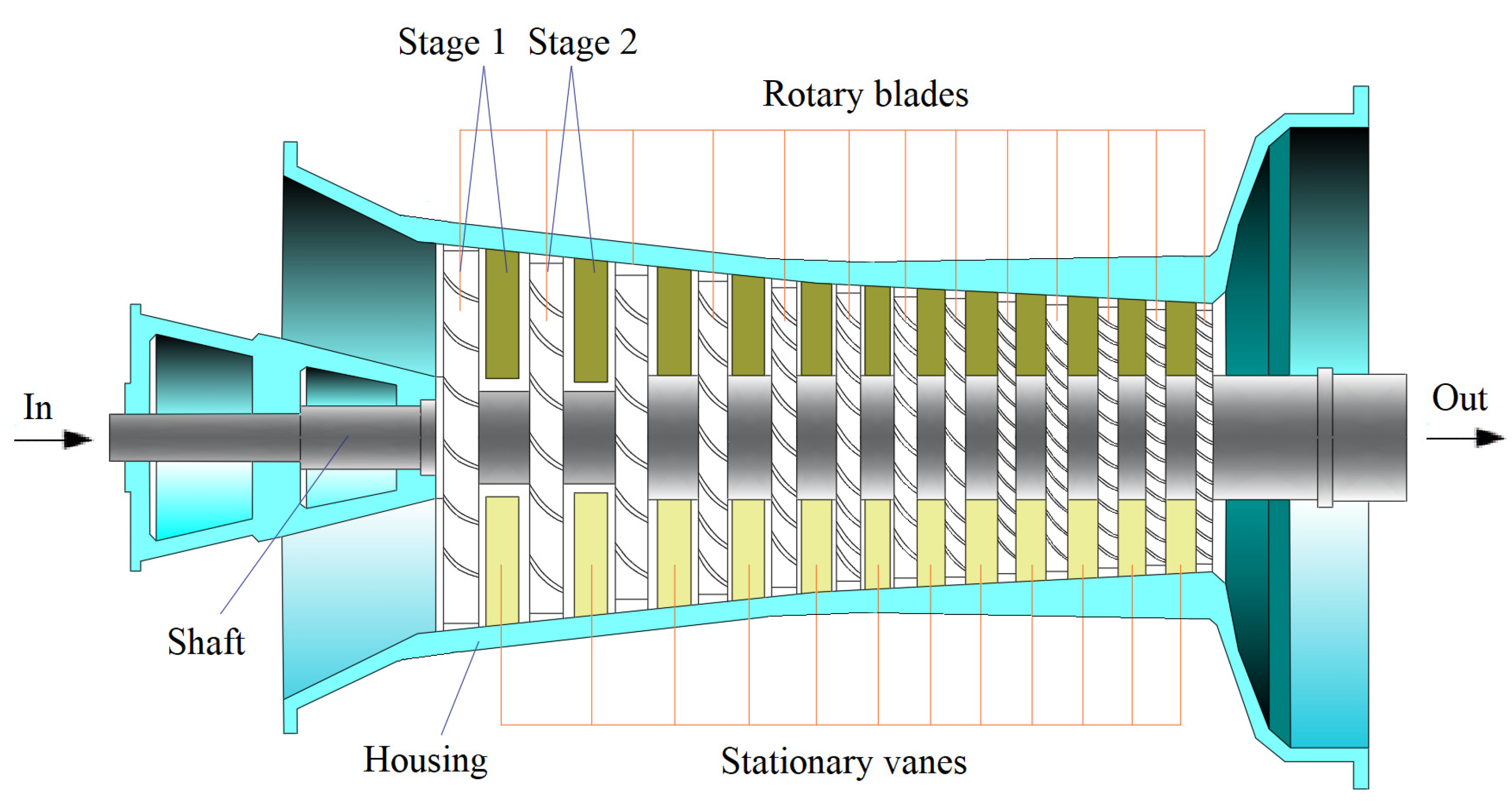
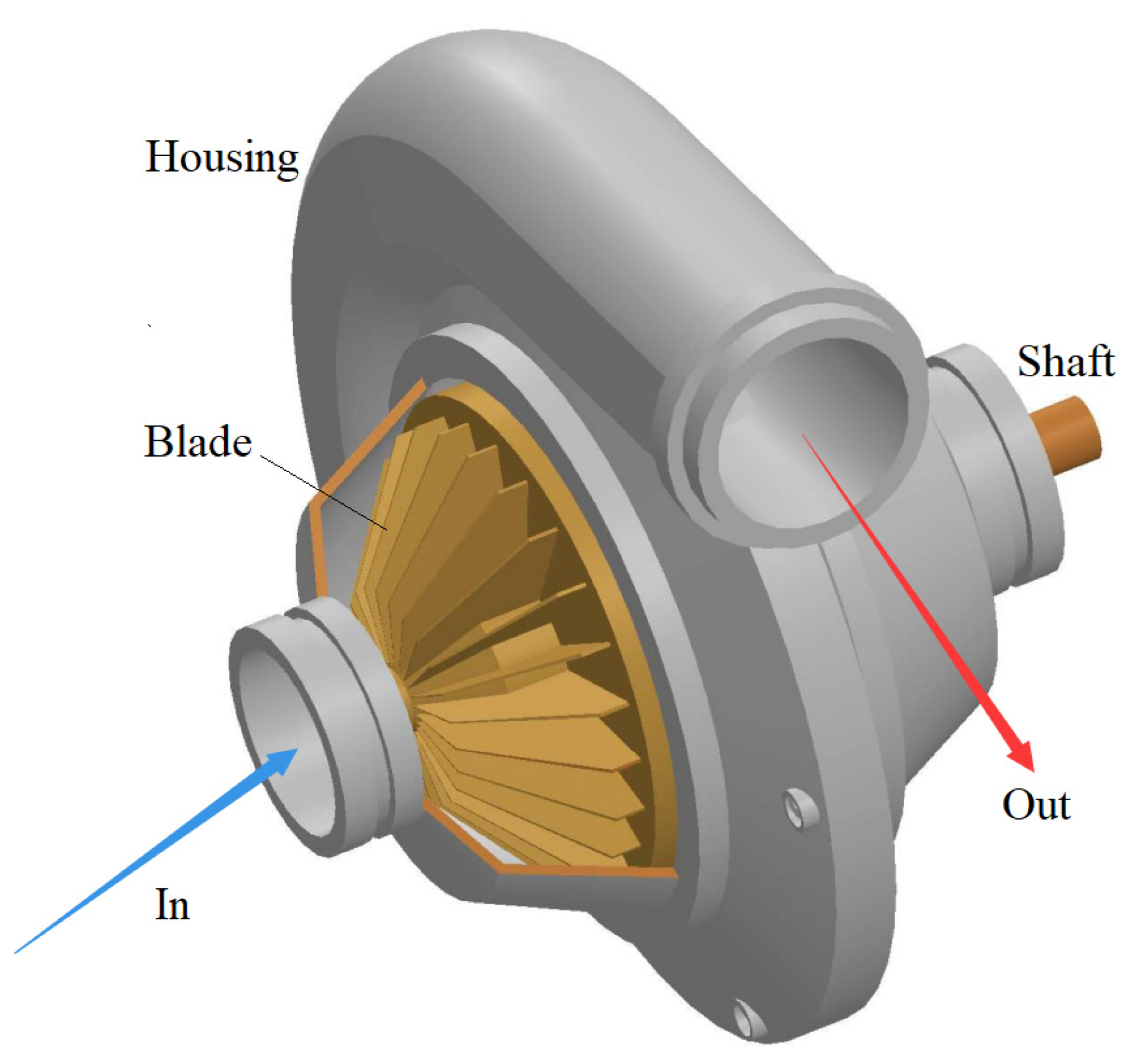
For a centrifugal compressor, gas enters it parallel to the shaft and leaves the blades radially. For an axial compressor, gas enters it and leaves the blades both parallel to the shaft. If gas enters a compressor parallel to the shaft and leaves the blades at an angle greater than 0° but less than 90° to the shaft, it is a mixed type. Figure 2 shows schematically a multi-stage axial compressor. Figure 3 shows schematically a single-stage centrifugal compressor.

3.3. Performance Maps of Dynamic Compressors

Three dynamic compressors are chosen for this study, with two from a civil turbofan engine named BIGFAN and the third from an airliner three-wheel high pressure water separator (HPWS) ECS. The BIGFAN engine compressors are multi-stage axial compressors, a commonly seen type in aero engines. The BIGFAN engine is a civil turbofan engine simulated in NLR’s Gas turbine Simulation Program (GSP) version 11 [46]. The ECS compressor is a single-stage centrifugal compressor used in Fokker 100 airliner, a regional jet that was produced by Fokker in Amsterdam, the Netherlands. Single-stage centrifugal compressors are a commonly seen type of compressors used in aircraft ECS.

3.3.1. Performance Maps of BIGFAN Compressors

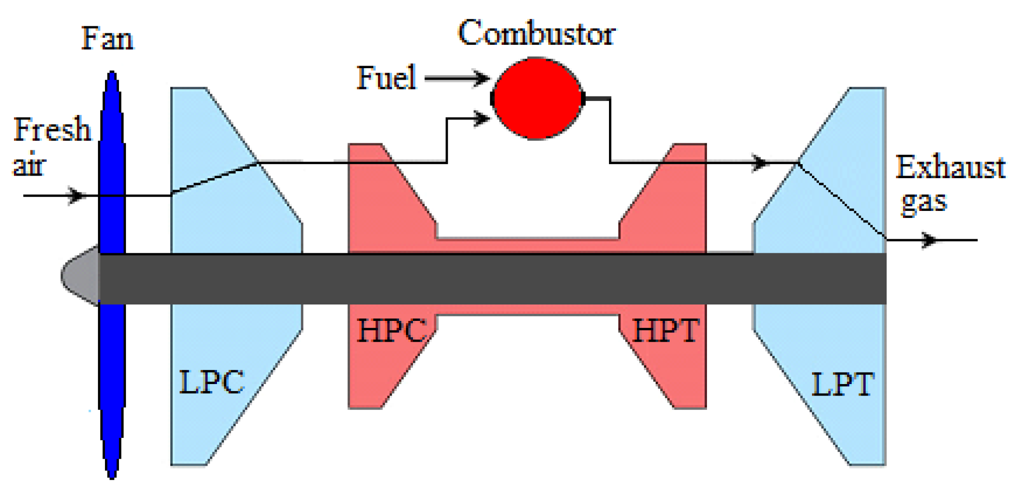
The main components of a BIGFAN include, in air flow direction, a fan, a low-pressure compressor (LPC), a high-pressure compressor (HPC), a combustor, a high-pressure turbine (HPT), and a low-pressure turbine (LPT) [46,47,48], as shown in Figure 4. The LPC is mounted on one shaft driven by the LPT, and the HPC is mounted on the high-pressure shaft driven by the HPT.

The fan delivers the compressed air to the compressors, where air pressure is increased gradually, coming out of the HPC as high-pressure hot air. The high-pressure hot air enters the combustor, or combustion chamber, where fuel is added. The air temperature increases remarkably in the combustor due to the combustion of air–fuel mixture, and then it enters the HPT and LPT in sequence, where it expands, producing the needed power.

The performance maps of the BIGFAN compressors were generated using the NLR’s GSP version 11 [46,47]. The performance map of the BIGFAN LPC is shown in Figure 5. The parameter ranges are the compression ratio π_c from 1.07 to 1.96, the corrected mass flow rate ϕ_corr from 19.2 to 107.8 kg/s, the isentropic efficiency η from 0.62 to 0.94, and the rotational speed ratio n_r from 0.3 to 1.2.

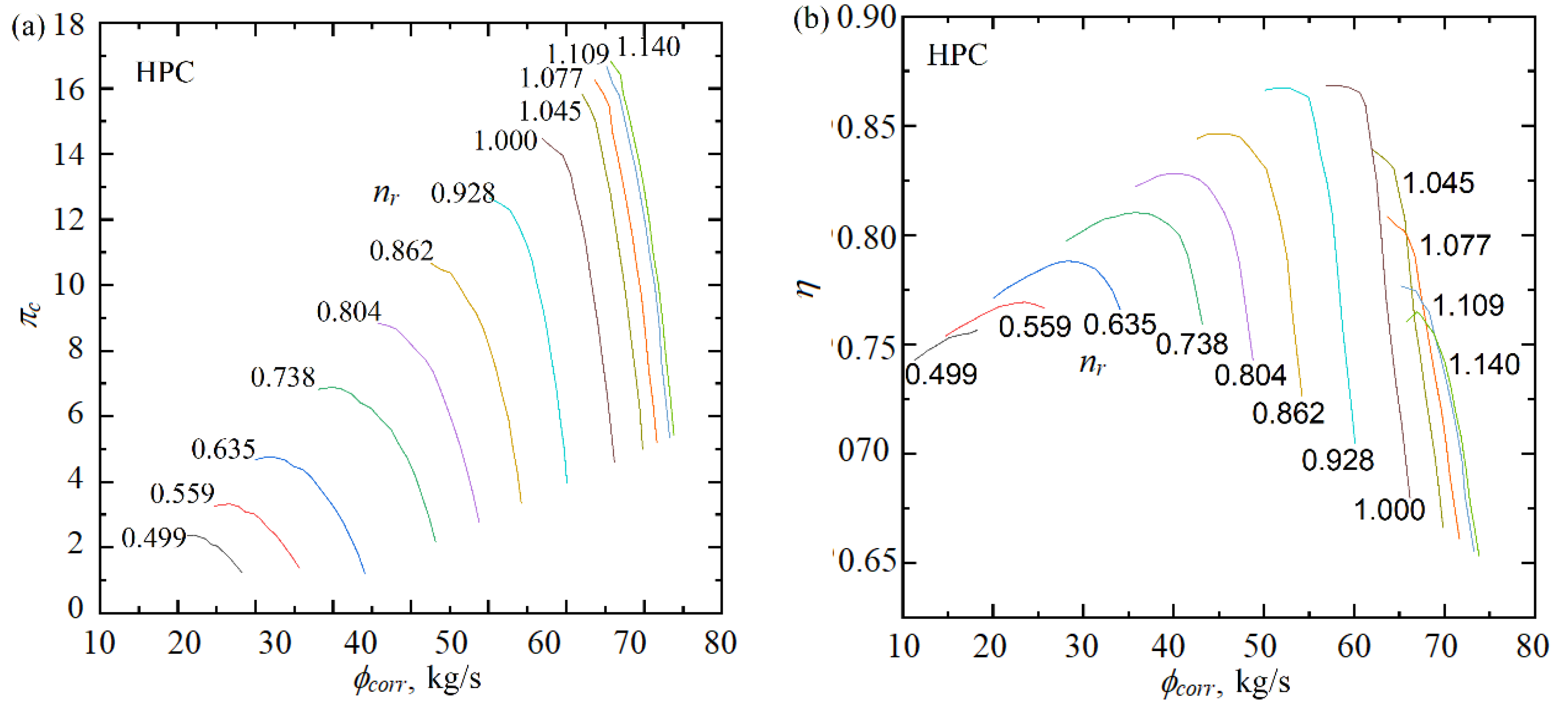
The performance map of the BIGFAN HPC is shown in Figure 6. The parameter ranges are the compression ratio π_c from 1.21 to 16.82, the corrected mass flow rate ϕ_corr from 20 to 65.7 kg/s, the isentropic efficiency η from 0.65 to 0.87, and the rotational speed ratio n_r from 0.5 to 1.14.

3.3.2. Performance Map of Aircraft ECS Compressor

For aircraft ECSs, dynamic compressors are used in air cycle machines (ACMs), vapor cycle refrigeration systems, and electric-driven air sources [2]. An ACM, which is composed of one or two cooling turbines with a compressor, a fan, or both on the same shaft to utilize the turbine work [49,50,51], is the key component of an air cycle ECS. The compressor of an ACM is either centrifugal, axial, or mixed dynamic, with the centrifugal type dominant.

An airliner HPWS ECS with a three-wheel ACM is shown schematically in Figure 7, which utilizes main engine bleed air as the pressurized air source and ram air as the heat sink [2]. The HPWS contains a condenser (COND), a reheater (REH), and a water extractor (WE). The bleed air passes through the primary heat exchanger (PHX), where it is cooled down. Then, it enters the ACM compressor (C), where its pressure is boosted. Leaving the compressor, the air is further cooled by the secondary heat exchanger (SHX). Coming out the SHX, it sequentially passes through the RHE hot side, the COND hot side, the WE, the RHE cold side, the ACM turbine (T), and the COND cold side, becoming cold air. The cold air mixes with the recirculation air from the cabin, and then the mixture enters the cabin, and eventually discharged overboard.

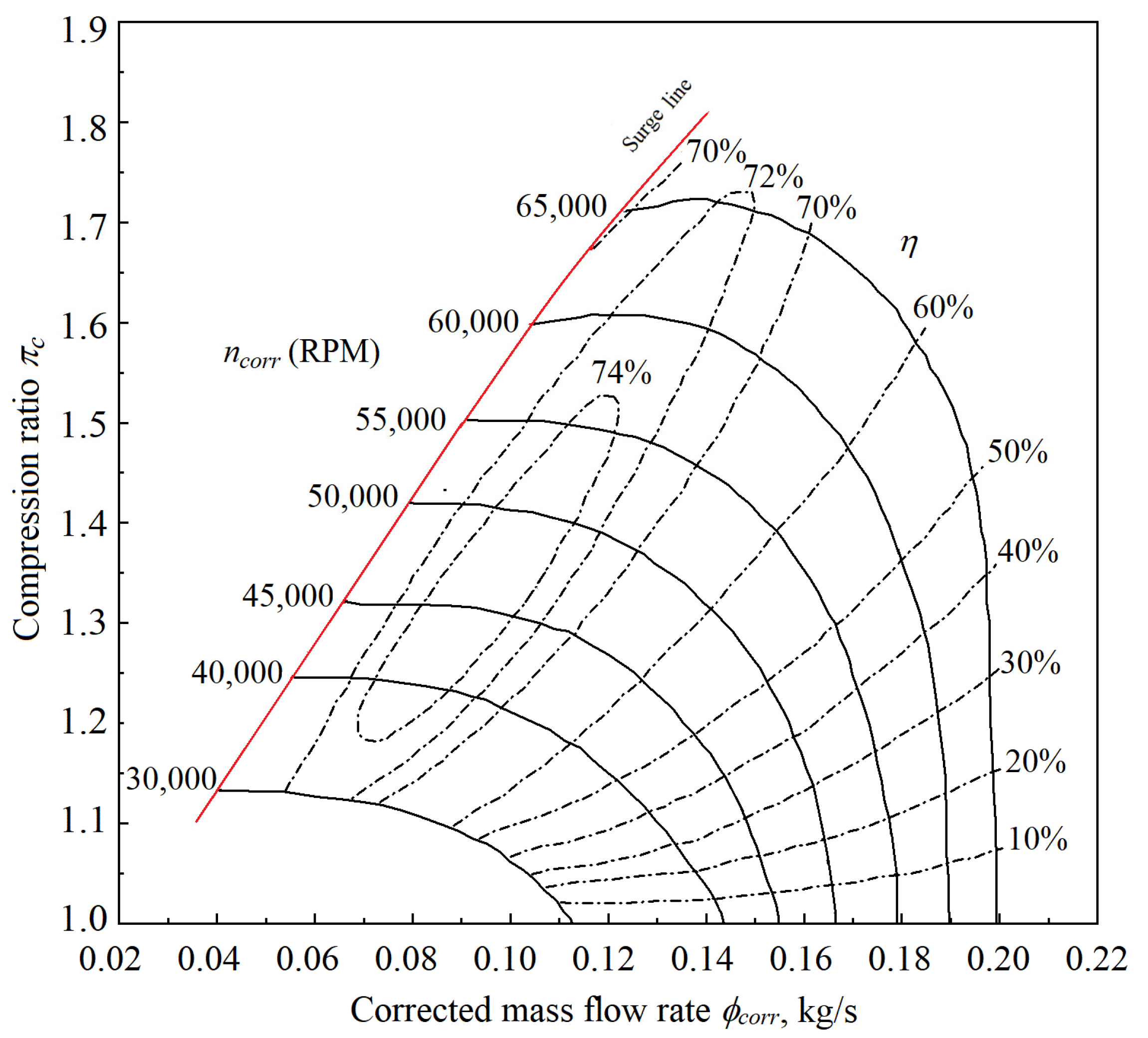
The performance map of an airliner ECS compressor is taken from [45], as shown in Figure 8. The data were read from the map using a computer software. The parameter ranges are the compression ratio π_c from 1.02 to 1.73, the corrected mass flow rate ϕ_corr from 0.04 to 0.2 kg/s, the isentropic efficiency η from 0.1 to 0.75, and the corrected rotational speed n_corr from 30,000 to 65,000 RPM.

3.4. Evaluation of the Existing Mass Flow Models

The evaluation results of the above-reviewed mass flow models against the BIGFAN LPC, the BIGFAN HPC, and the ECS compressor are shown in

Table 3. Mass flow models applied to the BIGFAN LPC.

Model	MAD (%)	Rc2
Tian [44]	2.0	0.954
Jiang et al. [40]	2.2	0.930
Guzzella and Amstutz [39]	2.9	0.938
Orkisz and Stawarz [42]	3.5	0.988
Eriksson et al. [38]	5.2	0.974
Jensen et al. [13]	6.3	0.962
Tsoutsanis et al. [35,36]	12.7	0.870
Tu and Chen [26]	12.8	0.865

,

Table 4. Mass flow models applied to the BIGFAN HPC.

Model	MAD (%)	Rc2
Orkisz and Stawarz [42]	2.1	0.997
Jensen et al. [13]	4.1	0.989
Tsoutsanis et al. [35,36]	4.9	0.988
Eriksson et al. [38]	5.1	0.989
Tu and Chen [26]	7.5	0.966
Jiang et al. [40]	10.2	0.827
Tian [44]	11.0	0.893

and

Table 5. Mass flow models applied to the ECS compressor.

Model	MAD (%)	Rc2
Tian [44]	2.4	0.960
Jiang et al. [40]	3.0	0.994
Tu and Chen [26]	4.5	0.945
Sieros et al. [43] model 1	5.2	0.922
Jensen et al. [13]	8.1	0.986
Biteus [37]	10.9	0.748
Kolmanovsky et al. [33,34]	11.0	0.741

, respectively, where only the models with MAD < 15% are listed.

From Table 3, Table 4 and Table 5, the following conclusions can be obtained:

• None of the evaluated existing mass flow models has an MAD less than 2.0%, indicating the need to develop new models with high accuracy.
• The Tian [44] model has the highest prediction accuracy for the BIGFAN LPC and the ECS compressor, with MADs of 2.0% and 2.4%, respectively, while it predicts poorly for the BIGFAN HPC, with an MAD of 11.0%. The Orkisz and Stawarz [42] model has the highest prediction accuracy for the BIGFAN HPC, with MAD = 2.1%, and a moderate prediction accuracy for the BIGFAN LPC, with an MAD of 3.5%, while it predicts poorly for the ECS compressor, with an MAD of 15%.
• The BIGFAN LPC is a multi-stage axial compressor, with ϕ_corr = 19.2–107.8 kg/s and π_c = 1.07–1.96. The BIGFAN HPC is a multi-stage axial compressor, with ϕ_corr = 20–65.7 kg/s and π_c = 1.21–16.82. The ECS compressor is a centrifugal compressor, with ϕ_corr = 0.04–0.2 kg/s and π_c = 1.02–1.73. Comparing the compressor type, mass flow rate, and the compression ratio, from the prediction accuracy of the Tian [44] model and the Orkisz and Stawarz [42] model to the three compressors, it may be reasoned that, among the three factors, the compression ratio and the compressor type rank in the first and the second places as to the effect on model applicability, and a single mass flow rate model may not be adequate to variety of applications.
• For evaluating the applicability of compressors, the MAD is much better than R_c². This can be seen by comparing the prediction accuracy of the Tian [44] model and that of Jensen et al. [13]. For the BIGFAN LPC and the ECS compressor, the Jensen et al. [13] model has higher R_c² values than the Tian [44] model, but actually the predictions of the Jensen et al. [13] model has much larger deviation from the map values than the Tian [44] model has.

3.5. Evaluation of the Existing Isentropic Efficiency Models

The evaluation results of the above-reviewed efficiency models against the BIGFAN LPC, the BIGFAN HPC, and the ECS compressor are shown in

Table 6. Isentropic efficiency models applied to the BIGFAN LPC.

Model	MAD (%)	Rc2
Tian [44]	1.8	0.911
Jiang et al. [40]	2.4	0.657
Park et al. [41]	2.5	0.815
Orkisz and Stawarz [42]	3.1	0.724
Guzzella and Amstutz [39]	3.2	0.654
Tsoutsanis et al. [35,36]	3.4	0.667
Sieros et al. [43] model 3	4.6	0.540
Eriksson et al. [38]	5.7	0.542

,

Table 7. Isentropic efficiency models applied to the BIGFAN HPC.

Model	MAD (%)	Rc2
Tian [44]	0.8	0.956
Park et al. [41]	1.6	0.902
Orkisz and Stawarz [42]	1.7	0.911
Jiang et al. [40]	1.8	0.852
Tsoutsanis et al. [35,36]	2.0	0.828
Eriksson et al. [38]	2.4	0.796
Sieros et al. [43] model 3	2.8	0.744
Guzzella and Amstutz [39]	3.5	0.779

and

Table 8. Isentropic efficiency models applied to the ECS compressor.

Model	MAD (%)	Rc2
Tian [44]	3.2	0.982
Sieros et al. [43] model 2	7.0	0.954
Sieros et al. [43] model 3	8.5	0.871
Park et al. [41]	8.5	0.935

, respectively, where only the models with MAD < 15% are listed.

All the mass flow rates in the efficiency maps of the BIGFAN LPC, the BIGFAN HPC, and the ECS compressor are given in the corrected mass flow parameter ϕ_corr, with the inlet temperature T_in and inlet pressure p_in not available, while the Tu and Chen [26] model uses volume flow rate Q, and thus it is not applicable theoretically and does not appear in the tables.

From Table 6, Table 7 and Table 8, the following points can be seen:

• The Tian [44] model has the highest prediction accuracy for all the three compressors, with MAD = 1.8% for the BIGFAN LPC, MAD = 0.8% for the BIGFAN HPC, and MAD = 3.2% for the ECS compressor, suggesting that it is possible to propose a single efficiency model for a wide range of applications.
• For the ECS compressor, the highest prediction accuracy of the existing models is MAD = 3.2% and, for the BIGFAN LPC, the highest prediction accuracy of the existing models is MAD = 1.8%, indicating a need to develop a highly accurate efficiency model.

4. Development of New Empirical Models for Dynamic Compressor Performance

The above-mentioned three performance maps of the dynamic compressors are used to test and tune the basic forms.

4.1. New Empirical Models of Mass Flow Rate

4.1.1. Developing New Models

Several data-driven methods are tried to develop new empirical models of mass flow rate, among which two effective examples are introduced below.

Method 1

The performance maps of the three compressors show that the corrected mass flow parameter ϕ_corr is the function of the compression ratio π_c and the corrected rotational speed n_corr, or π_c is the function of the ϕ_corr and n_corr. Thus, it follows that

$${\varphi }_{corr}=f({\pi }_c,n_{corr})$$

(17)

or

$${\pi }_c=f({\varphi }_{corr},n_{corr})$$

(18)

Assuming that f(π_c, n_corr) is the function of the product of the sub-function f₁(π_c, n_corr), f₂(π_c, n_corr), …, f_k(π_c, n_corr), Equation (17) becomes

$${\varphi }_{corr}=f_1({\pi }_c,n_{corr})f_2({\pi }_c,n_{corr})\dots f_{\mathrm{k}}({\pi }_c,n_{corr})$$

(19)

where f_i(π_c, n_corr) (i = 1, 2, …, k) have very complicated forms due to the complicated compressor configurations and the flow fields in compressor channels.

So far, it is impossible to derive an explicit equation for f_i(π_c, n_corr) through theoretical analysis, and thus data-driven methods have to be used to find the right forms. Generally, a variety of the basic forms of empirical correlations need to be constructed and then tested through computation based on the available compressor performance data. The following steps are adopted to determine mass flow rate model forms:

• Choose a k value. For example set k = 3.
• Construct sub-functions f₁(π_c, n_corr), f₂(π_c, n_corr), and f₃(π_c, n_corr). The simplest practice is to use polynomial forms.
• Based on the above-mentioned three performance maps of mass flow rate, conduct extensive computational trial and error using different data-driven methods. Those yielding superior results are selected to refine the sub-functions in the next step. In this step, the tested data-driven methods include the Levenberg–Marquardt method, the Powell Optimization method, the Quasi-Newton method, the Simplex method, the Gold Rush Optimizer, the Python curve fit tool, and the Genetic Algorithm (GA). The Levenberg–Marquardt method, the Python curve fit tool, and GA show superior performance, and are selected to refine the sub-functions in the next step.
• Use MAD as the criterion to tune the sub-functions using the data-driven methods selected in the above step. In this step, add or remove terms in the sub-functions one by one to determine which terms should be included. If removing a term does not increase MAD, this term should be removed. If adding a term does not reduce MAD, this term should not be added. The general model form include all terms for the three compressors.
• If the result obtained in the above step is unsatisfactory, go to step 1 and repeat the processes of trial and error in steps 1–4, until a satisfied result is obtained.

Regarding the use of GA, the initial number of populations is 300–500, the number of iterations is 2000–4000, the crossover probability is 0.85, and the variance probability is 0.1. The sub-generation of individuals with the smallest MAD without R_c² deterioration is the optimal one after the iteration. The data is split into two groups, one with 75% of the total data, and the other with 25%, similar to the training set and test set in machine learning. The training set, which contains 75% of the total data, is used to obtain the model, and then the model is used to predict the test set. The resultant MAD is the weighted arithmetic mean of the MADs of the two data sets.

The final general model yielded by this method is of the form

$${\varphi }_{corr}={\displaystyle \frac{a_0+a_1{\pi }_c+a_2{n}_{corr}+a_3{\pi }_c^2+a_4{n_{corr}}^2+a_5{\pi }_c{n}_{corr}+a_6{\pi }_c^3+a_7{n_{corr}}^3+a_8{\pi }_c{n_{corr}}^2}{1+a_9{\pi }_c+a_{10}{n}_{corr}+a_{11}{\pi }_c^2+a_{12}{n_{corr}}^2+a_{13}{\pi }_c{n}_{corr}+a_{14}{\pi }_c^3+a_{15}{n_{corr}}^3+a_{16}{\pi }_c^2{n}_{corr}}}$$

(20)

where a_i (i = 1, 2, …, 16) are the constants to be determined by the available data.

Mention should be made of the fact that the above equation is a general form for the mass flow rate of dynamic compressors. Some terms may be removed to simplify the form for a given compressor. It is suggested to remove as many terms as possible to simplify the model for a given compressor. The suggest methodology is as follows.

At first, remove one term, if necessary, from the general form. Test each term in the general form by removing it while keeping all the other terms to calculate the MAD and the R_c² of the reduced model. Divide all the terms into three categories: strong relevant terms, weak relevant terms, and little relevant terms. A term is strong relevant if the MAD increases remarkably when removing it from the model, a term is weak relevant if the MAD increases noticeably when removing it from the model, and a term is little relevant if the MAD increases very little or does not increase when removing it from the model. Among the little relevant terms, the one yielding the smallest MAD and the greatest or almost greatest R_c² when removed should be deleted from the general form. For convenience, the model yielded in this round is called the first-generation model. Generally, for a given compressor, at least one term can be removed from the general form.

Secondly, test each term of the above-mentioned weak relevant and little relevant terms remaining in the first-generation model by removing it while keeping all the other terms to calculate the MAD and the R_c² of the further reduced model, and classify them into strong relevant terms, weak relevant terms, and little relevant terms. Among the little relevant terms, if any, the one yielding the smallest MAD and the greatest or almost greatest R_c² when removed may be deleted from the first-generation model. The model yielded in this round is called the second-generation model. Please note that a strong relevant term, no matter in which round it is yielded, remains as a strong relevant term in the next round, and all strong relevant terms are kept in the model, exempt from testing.

In the second round, if there is no little relevant term, the first-generation model is the final result. If not, try to reduce the second-generation model using the same method as that when reducing the first-generation model. Repeat this method until no term can be removed.

With this approach, the final mass flow rate model and accuracy for the three compressors are obtained, as listed in

Table 9. Final mass flow rate model form and accuracy for the three compressors.

Compressor	MAD (%)	Rc2	Terms Removed from Equation (20)
BIGFAN LPC	1.1	0.9981	a6, a13
BIGFAN HPC	1.3	0.9988	a7, a11, a14
ECS compressor	2.8	0.9827	a4, a5, a6, a13

, where the terms with the constants in the “Terms removed from Equation (20)” column are removed from Equation (20).

Method 2

Equation (20) has very high accuracy for the BIGFAN LPC and BIGFAN HPC, but it falls short of predicting the ECS compressor satisfactorily. Therefore, a need exists to develop another mass flow rate model with high prediction accuracy for the ECS compressor, which is of the centrifuge type and operates at low compression ratio.

Observing the ECS compressor performance map in Figure 8, it is found that, for a given corrected rotational speed n_corr, the compression ratio π_c is the exponential function of the corrected mass flow parameter ϕ_corr, and thus it follows that

$${\pi }_c=A{e}^{B{\phi }_{corr}}+C$$

where A, B, and C can be expressed as the function of corrected rotational speed n_corr.

Through extensive computer test, the polynomial function for A, B, and C yields preferable results. The obtained final form of mass flow rate is as follows:

$$\begin{array}{l}{\pi }_c=A_1{e}^{A_2{\phi }_{corr}}+A_3\\ A_i=a_{i,1}{n_{corr}}^2+a_{i,2}{n}_{corr}+a_{i,3}\end{array}$$

(21)

where the constants a_i,j (i = 1, 2, 3, and j = 1, 2, 3) are to be determined by the available data.

The prediction ability of Equation (21) for the three compressors is shown in

Table 10. Prediction ability of Equation (21).

Compressor	MAD (%)	Rc2
ECS compressor	1.3	0.9808
BIGFAN LPC	2.0	0.9992
BIGFAN HPC	5.6	0.9952

. It is seen that this model has a high prediction accuracy for the ECS compressor, and its prediction ability for the BIGFAN LPC is fairly good.

From the compressor type, it is reasoned that Equation (20) may be better for multi-stage axial compressors and Equation (21) may be better for centrifugal compressors. However, for a given compressor, it is suggested that careful computer tests should be conducted to determine which model is better.

4.1.2. Comparison of the New Models with the Best Existing Models

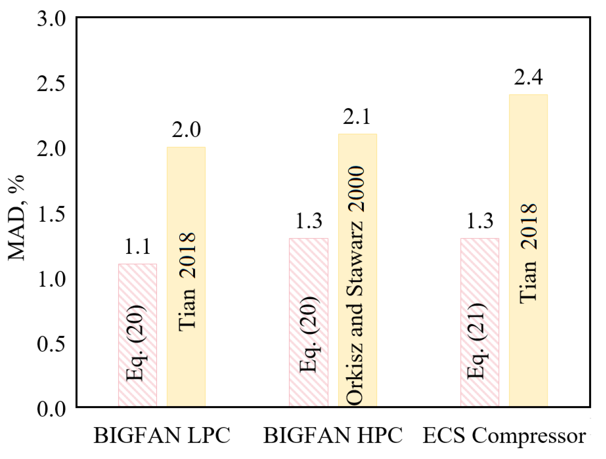
Figure 9 shows the comparison of the prediction errors (MAD) of the new mass flow models with the best existing ones in prediction accuracy, where Equations (20) and (21) are the new models, and Tian [44] and Orkisz and Stawarz [42] are the best existing models for the specified compressors. It is seen that the new models predict the three compressors with MAD ≤ 1.3%, while the best existing models all have MAD > 2.0%, indicating that the new models improve the prediction accuracy greatly.

4.2. New Empirical Model of Isentropic Efficiency

4.2.1. Developing New Model

From the evaluation of the isentropic efficiency models of dynamic compressors, it is seen that the Tian [44] model gives satisfied prediction results for the BIGFAN LPC and HPC, while no model predicts well for the ECS compressor. In practice, the available performance dada of aero engine and ECS compressors are usually given in the corrected mass flow rate ϕ_corr or the mass flow rate parameter ϕ without giving T_in and p_in information, leaving the volume flow rate Q unknown. Since T_in and p_in vary in real operation processes, it is necessary to propose a compressor efficiency model with ϕ_corr or ϕ instead of Q.

In order to find more clues for developing a said new efficiency model, the Tu and Chen [26] efficiency model was evaluated against the above-mentioned three efficiency maps by assuming that T_in and p_in are constant, from which the volume flow rate Q is calculated. The results show that the Tu and Chen [26] has very high prediction accuracy for the BIGFAN LPC and BIGFAN HPC, though its prediction accuracy is not high for the ECS compressor. By assuming that T_in and p_in are constant, the prediction accuracy of the Tu and Chen [26] model is overestimated.

Based on the above evaluation and analysis, several basic efficiency model forms were constructed. Through extensive computer testing, it is found that the best basic efficiency model form for a dynamic compressor is as follows:

$$\begin{array}{l}\eta =a_0+a_1{\varphi }_{corr}+a_2{\pi }_c+a_3{{\varphi }_{corr}}^2+a_4{\pi }_c^2+a_5{\varphi }_{corr}{\pi }_c+a_6{{\varphi }_{corr}}^3\\ +a_7{\pi }_c^3+a_8{{\varphi }_{corr}}^2{\pi }_c+a_9{\varphi }_{corr}{\pi }_c^2+a_{10}{{\varphi }_{corr}}^4+a_{11}{\pi }_c^4\\ +a_{12}{{\varphi }_{corr}}^3{\pi }_c+a_{13}{{\varphi }_{corr}}^2{\pi }_c^2+a_{14}{\varphi }_{corr}{\pi }_c^3+a_{15}{\pi }_c^5+a_{16}{\varphi }_{corr}{\pi }_c^4\end{array}$$

(22)

It should be mentioned that, for a given compressor, some terms in the above general form may be removed with little increase in MAD. In other words, some terms in Equation (22) may be removed to simplify the efficiency model for a given compressor. It is suggested to remove as many terms as possible for a given compressor as long as the R_c² value does not noticeably deteriorate.

The prediction accuracy of the new model for the BIGFAN LPC, the BIGFAN HPC, and the ECS compressor is listed in

Table 11. Prediction accuracy of the new efficiency model.

Compressor	MAD (%)	Rc2	Terms Removed from Equation (22)
BIGFAN LPC	1.0	0.9633	a6, a13
BIGFAN HPC	0.4	0.9922	a12
ECS compressor	1.9	0.9967	a13, a15

, where the terms with the constants in the “Terms removed from Equation (22)” column are removed from Equation (22).

4.2.2. Comparison of the New Model with the Best Existing Models

Figure 10 shows the comparison of the prediction errors (MAD) of the new isentropic efficiency model with the best existing model in prediction accuracy, where New means Equation (22) and Tian [44] denotes the Tian [44] compressor efficiency model, which predicts best for all of the three compressors. It is seen that the new model has a much higher prediction accuracy (much lower MAD) than the best existing model.

5. Conclusions and Discussion

The existing empirical formulas for dynamic compressors, including 16 mass flow rate models and 14 isentropic efficiency models, were evaluated against the performance data of two multi-stage axial compressors used in an aero engine and a centrifugal compressor used in an aircraft ECS. Two empirical formulas for mass flow rate and one for isentropic efficiency of dynamic compressors are proposed. The following conclusions are obtained:

• For three dynamic compressors, none of the existing empirical models of mass flow rate has an MAD less than 2.0%, and the smallest MAD of the existing isentropic efficiency models is 3.4%, indicating the need to develop new models with high accuracy.
• As to the effect on the applicability of mass flow rate models, compression ratio and compressor type rank in the first and the second places among the three factors of compressor type, mass flow rate, and the compression ratio. A single mass flow rate model may not be adequate to a variety of applications.
• A compressor efficiency model is less sensitive to compressor type, mass flow rate, and the compression ratio than a mass flow rate model. The Tian [44] model was developed for aircraft ECS centrifugal compressors with low compression ratio and small mass flow rate, but it has the highest prediction accuracy for multi-stage axial compressors in wide ranges of compression ratio and mass flow rate among the existing models.
• The data-driven method is used to develop new models of mass flow rate and isentropic efficiency for dynamic compressors, for which two empirical formulas (Equations (20) and (21)) for the mass flow rate and one (Equation (22)) for the isentropic efficiency are developed.
• The new models have much higher prediction accuracy than the best existing models. The new mass flow rate models predict the three compressors with MAD ≤ 1.3%, while the best existing models all have MAD > 2.0%. The new efficiency model predicts the BIGFAN LPC, BIGFAN HPC, and ECS compressor, with MAD of 1.0%, 0.4%, and 1.9%, respectively, while the best existing one predicts the BIGFAN LPC, BIGFAN HPC, and ECS compressor with MAD of 1.8%, 0.8%, and 3.2%, respectively.
• For evaluating the applicability of compressors, the criterion MAD is much better than R_c², while R_c² is preferred to refining a general form, with some terms needing to be removed or added.
• Most of the existing empirical models of mass flow rate and isentropic efficiency of dynamic compressors relate to dimensional parameters, which limits the model robustness. Modeling the characteristics by relying on the fundamentals of the theory of dynamic compressors may have potential to solve the problem.

References

1. Yang, B.; Fang, X.; Zhang, L.; Zhuang, F.; Bi, M.; Chen, C.; Li, G.; Wang, X. Applicability of empirical models of isentropic efficiency and mass flow rate of dynamic compressors to jet engines. Prog. Aerosp. Sci. 2019, 106, 32–42. [Google Scholar] [CrossRef]
2. Fang, X. Aircraft Environmental Control and Refrigeration; Beihang Press: Beijing, China, 2023. [Google Scholar]
3. Meira, R.L.; Costa, G.M.N.; Kalid, R.A.; Martins, M.A.F. Improving the centrifugal compressor map through rigorous thermodynamic modeling: An analysis on a natural gas compression station pipeline. J. Nat. Gas Sci. Eng. 2021, 92, 104006. [Google Scholar] [CrossRef]
4. Molière, M. The fuel flexibility of gas turbines: A review and retrospective outlook. Energies 2023, 16, 3962. [Google Scholar] [CrossRef]
5. Liu, Z.; Liu, X.; Yang, S.; Hooman, K.; Yang, X. Assessment evaluation of a trigeneration system incorporated with an underwater compressed air energy storage. Appl. Energy 2021, 303, 117648. [Google Scholar] [CrossRef]
6. Wang, Z.; Xiao, Y.; Li, X.; Ren, X.; Gu, C.; Li, Y. Experiment and numerical simulation of the performance on scaled compressor cascade and development of a prediction model. Int. J. Heat. Fluid. Flow. 2024, 105, 109243. [Google Scholar] [CrossRef]
7. Li, Z.; Agarwal, R.K. Numerical simulations and design optimization of compressor cascade flow using one equation and Wray-Agarwal turbulence model. Int. J. Comput. Fluid Dyn. 2022, 36, 705–718. [Google Scholar] [CrossRef]
8. Nicolas, V.; Sdanghi, G.; Mozet, K.; Schaefer, S.; Maranzana, G.; Celzard, A.; Fierro, V. Numerical simulation of a thermally driven hydrogen compressor as a performance optimization tool. Appl. Energy 2022, 323, 119628. [Google Scholar] [CrossRef]
9. Tsujikawa, G.S. Digital Controlled Closed Loop Air Cycle Development; SAE 851319; Society of Automobile Engineers, Inc.: Warrendale, PA, USA, 1985. [Google Scholar]
10. He, J.; Zhao, J.Q.; Sun, W. Dynamic simulation of bootstrap air cycle refrigeration components for aircraft environmental control system. J. Syst. Simul. 2004, 16, 727–729. [Google Scholar]
11. Yang, Y.; Chen, S.; Sheng, C.; Xie, H.; Luo, G.; Hou, Y. Study on coupling performance of turbo-cooler in aircraft. Energy 2021, 224, 120029. [Google Scholar] [CrossRef]
12. Jennions, I.; Ali, F.; Miguez, M.E.; Escobar, I.C. Simulation of an aircraft environmental control system. Appl. Therm. Eng. 2020, 172, 114925. [Google Scholar] [CrossRef]
13. Jensen, J.P.; Kristensen, A.F.; Sorenson, S.C.; Houbak, N.; Hendricks, E. Mean Value Modeling of a Small Turbocharged Diesel Engine; SAE 910070; Society of Automobile Engineers, Inc.: Warrendale, PA, USA, 1991. [Google Scholar]
14. Mueller, M. Mean Value Modeling of Turbocharged Spark Ignition Engines. Master′s Thesis, DTU, Kgs Lyngby, Denmark, 1997. [Google Scholar]
15. Canova, M.; Midlam-Mohler, S.; Guezennec, Y.; Rizzoni, G. Mean value modeling and analysis of HCCI diesel engines with external mixture formation. J. Dyn. Syst. Meas. Control. 2009, 131, 011002. [Google Scholar] [CrossRef]
16. Liu, M.; Wang, B.; Liu, D. A digital twin modeling method for turbofan engine real-time test data analysis and performance monitoring. In Proceedings of the 2020 11th International Conference on Prognostics and System Health Management (PHM-2020), Virtual Meeting, 16–18 October 2020. [Google Scholar]
17. Zhang, Z.J.; Duraisamy, K. Machine learning methods for data-driven turbulence modeling. In Proceedings of the 22nd AIAA Computational Fluid Dynamics Conference, Dallas, TX, USA, 22–26 June 2015. [Google Scholar]
18. Ahmad, T.; Chen, H.; Guo, Y.; Wang, J. A comprehensive overview on the data driven and large scale based approaches for forecasting of building energy demand: A review. Energy Build. 2018, 165, 301–320. [Google Scholar] [CrossRef]
19. Pulpeiro Gonzalez, J.; Hall, C. Equation-Based Compressor and Turbine Modeling for Variable Geometry Turbochargers; SAE Technical Paper 2018-01-0966; SAE: Warrendale, PA, USA, 2018. [Google Scholar] [CrossRef]
20. Sun, J.; Li, C.; Liu, C.; Gong, Z.; Wang, R. A data-driven health indicator extraction method for aircraft air conditioning system health monitoring. Chin. J. Aeronaut. 2019, 32, 409–416. [Google Scholar] [CrossRef]
21. Fang, X.; Dai, Q. Modeling of turbine mass flow rate performances using the Taylor expansion. Appl. Therm. Eng. 2010, 30, 1824–1831. [Google Scholar] [CrossRef]
22. Fang, X.; Xu, Y. Development of an empirical model of turbine efficiency using the Taylor expansion and regression analysis. Energy 2011, 36, 2937–2942. [Google Scholar] [CrossRef]
23. Nikiforov, A.; Popova, D.; Soldatova, K. A network application for modeling a centrifugal compressor performance map. IOP Conf. Ser. Mater. Sci. Eng. 2017, 232, 012046. [Google Scholar] [CrossRef]
24. Fei, J.; Zhao, N.; Shi, Y.; Feng, Y.; Wang, Z. Compressor performance prediction using a novel feed-forward neural network based on Gaussian kernel function. Adv. Mech. Eng. 2016, 8, 1–14. [Google Scholar] [CrossRef]
25. Uzun, M.; Demirezen, M.U.; Inalhan, G. Physics guided deep learning for data-driven aircraft fuel consumption modeling. Aerospace 2021, 8, 44. [Google Scholar] [CrossRef]
26. Tu, H.; Chen, H. Modeling of a compressor’s performance map by fitting function methodology. Adv. Mater. Res. 2013, 779–780, 1194–1198. [Google Scholar] [CrossRef]
27. Li, X.; Yang, C.; Wang, Y.; Wang, H. A prediction model of compressor with variable-geometry diffuser based on elliptic equation and partial least squares. R. Soc. Open Sci. 2018, 5, 171468. [Google Scholar] [CrossRef]
28. Yang, H.; Yang, C. Application of scaling-endoreversible thermodynamic analysis model to aircraft environmental control system-methodology development. Int. J. Refrig. 2020, 112, 90–99. [Google Scholar] [CrossRef]
29. Chen, S.; Zuo, S.; Wu, Z. Aerodynamic performance modeling of the centrifugal compressor and stability analysis of the compression system for fuel cell vehicles. SAE Int. J. Adv. Curr. Pract. Mobil. 2021, 3, 2325–2336. [Google Scholar] [CrossRef]
30. Canova, M. Development and validation of a control-oriented library for the simulation of automotive engines. Int. J. Engine Res. 2004, 5, 219–228. [Google Scholar] [CrossRef]
31. Fang, X.; Chen, W.; Zhou, Z.; Xu, Y. Empirical models for efficiency and mass flow rate of centrifugal compressors. Int. J. Refrig. 2014, 41, 190–199. [Google Scholar] [CrossRef]
32. Andersson, P. Air Charge Estimation in Turbocharged Spark Ignition Engines. Ph.D. Thesis No. 989, Department of Electrical Engineering, Linkoping University, Linkoping, Sweden, 2005. [Google Scholar]
33. Kolmanovsky, I.V.; Moraal, P.E.; van Nieuwstadt, M.J.; Criddle, M.; Wood, P. Modeling and Identification of a 2.0 L Turbocharged DI Diesel Engine; Ford Internal Technical Report SR-97-039; Ford: Dearborn, MI, USA, 1997. [Google Scholar]
34. Moraal, P.; Kolmanovsky, I. Turbocharger modeling for automotive control application. SAE Trans. 1999, 108, 1324–1338. [Google Scholar]
35. Tsoutsanis, E.; Meskin, N.; Benammar, M.; Khorasani, K. A component map tuning method for performance prediction and diagnostics of gas turbine compressors. Appl. Energy 2014, 135, 572–585. [Google Scholar] [CrossRef]
36. Tsoutsanis, E.; Meskin, N.; Benammar, M.; Khorasani, K. Transient gas turbine performance diagnostics through nonlinear adaptation of compressor and turbine maps. J. Eng. Gas Turbines Power 2015, 137, 091201. [Google Scholar] [CrossRef]
37. Biteus, J. Mean Value Engine Model of a Heavy Duty Diesel Engine; LITH-ISY-R-2666; Department of Electrical Engineering, Linkopings Universitet: Linkoping, Sweden, 2004. [Google Scholar]
38. Eriksson, L.; Nielsen, L.; Brugard, J.; Bergstriim, J.; Pettersson, F.; Andersson, P. Modeling of a turbocharged SI engine. Annu. Rev. Control. 2002, 26, 129–137. [Google Scholar] [CrossRef]
39. Guzzella, L.; Amstutz, A. Control of diesel engines. IEEE Control. Syst. Mag. 1998, 18, 53–71. [Google Scholar]
40. Jiang, H.; Dong, S.; Liu, Z.; He, Y.; Ai, F. Performance prediction of the centrifugal compressor based on a limited number of sample data. Math. Probl. Eng. 2019, 2019, 5954128. [Google Scholar] [CrossRef]
41. Park, Y.; Park, I.; Min, K.; Sunwoo, M. Model-based feedforward control of the VGT in a diesel engine based on empirical models of compressor and turbine efficiencies. Int. J. Automot. Technol. 2015, 16, 561–570. [Google Scholar] [CrossRef]
42. Orkisz, M.; Stawarz, S. Modeling of turbine engine axial-flow compressor and turbine characteristics. J. Propuls. Power 2000, 16, 336–339. [Google Scholar] [CrossRef]
43. Sieros, G.; Stamatis, A.; Mathioudakis, K. Jet engine component maps for performance modeling and diagnosis. J. Propuls. Power 1997, 13, 665–674. [Google Scholar] [CrossRef]
44. Tian, L. Research on Mathematical Modeling of Fault Prediction of Aircraft Environmental Control System. Master’s Thesis, Nanjing University of Aeronautics and Astronautics, Nanjing, China, 2018. [Google Scholar]
45. Yang, Y. Simulation Research on Mean Value Model of Air Circulation Machine and Aircraft Environmental Control System. Master’s Thesis, Nanjing University of Aeronautics and Astronautics, Nanjing, China, 2020. [Google Scholar]
46. NLR. Program GSP 11; National Aerospace Laboratory NLR: Amsterdam, The Netherlands, 2014. [Google Scholar]
47. Yang, B. Research on Adaptive Control of Turbofan Engine Based on Data Driven. Ph.D. Thesis, Beihang University, Beijing, China, 2021. [Google Scholar]
48. Sun, P.; Fang, X.; Zhuang, F.; Chen, C.; Shang, H.; Liu, Y.; Yang, B. Evaluation of applicability of empirical models of turbine performance to aircraft engine. Aerosp. Sci. Technol. 2021, 117, 106953. [Google Scholar] [CrossRef]
49. Jones, K.; Claeys, H. The Continuing Evolution of the C-130 Environmental Control System; SAE 1999-01-2163; Society of Automobile Engineers, Inc.: Warrendale, PA, USA, 1999. [Google Scholar]
50. Ryan, S.K. F-15 Environmental System Improvements; SAE 901235; Society of Automobile Engineers, Inc.: Warrendale, PA, USA, 1990. [Google Scholar]
51. Wiegand, C.; Bullick, B.A.; Catt, J.A.; Hamstra, J.W.; Walker, G.P.; Wurth, S. F-35 air vehicle technology overview. In Proceedings of the AIAA Aviation Forum, Atlanta, GA, USA, 25–29 June 2018. [Google Scholar]
Figure 1. Types of dynamic compressors.
Aerospace 11 00589 g001
Figure 2. Schematics of an axial dynamic compressor.
Aerospace 11 00589 g002
Figure 3. Schematics of a single-stage centrifugal dynamic compressor.
Aerospace 11 00589 g003
Figure 4. Schematic diagram of turbofan engine (BIGFAN).
Aerospace 11 00589 g004
Figure 5. Performance map of the BIGFAN LPC [47]. (a) Performance map of mass flow rate. (b) Performance map of isentropic efficiency.
Aerospace 11 00589 g005
Figure 6. Performance map of the BIGFAN HPC [47]. (a) Performance map of mass flow rate. (b) Performance map of isentropic efficiency.
Aerospace 11 00589 g006
Figure 7. Schematic diagram of three-wheel HPWS ECS [2].
Aerospace 11 00589 g007
Figure 8. Performance map of the ECS compressor [45].
Aerospace 11 00589 g008
Figure 9. Prediction MAD: New mass flow models vs. the best existing ones (Tian [44] for BIGFAN LPC and ECS compressor, Orkisz and Stawarz [42] for BIGFAN HPC).
Aerospace 11 00589 g009
Figure 10. Prediction MAD: New efficiency model vs. the best existing one (Tian [44]).
Aerospace 11 00589 g010