Numerical Simulation of the Transient Thermal Load of a Sightseeing Airship Cockpit

Abstract

The calculation of a cockpit’s transient thermal load is important for determining the capacity of the cockpit environmental control system, ensuring the safety of electronic equipment and increasing the health and comfort of cockpit occupants. According to the structural parameters of the cockpit of a sightseeing airship, a physical model is established. The turbulence model and calculation method are selected and verified. The transient thermal load within full flight envelope, the cockpit thermal loads at different times of the day, and the cockpit thermal loads under different free-flow velocities are obtained based on the Computational Fluid Dynamics (CFD) method. The cockpit transient thermal loads during different seasons are also obtained. The results show that solar radiation has a great influence on the cockpit transient thermal load. As the flight altitude increases, the thermal load decreases from 8.8 kW (H = 0 m) to 4.7 kW (H = 3000 m). With the change in the solar radiation intensity and solar radiation angle, the thermal load increases considerably, from 2.2 kW (8:00 a.m.) to 5.4 kW (12:00 a.m.). The influence of the free-flow velocity is not very obvious at an altitude of 3000 m, as discussed in this study. The influence of seasons is significant. Finally, the influence of the solar absorptivity and infrared emissivity of the cockpit surface material are studied, and the temperature distribution on the cockpit’s surface is determined.

1. Introduction

The temperature inside the cockpit of an airship is influenced by the interior and exterior thermal loads. The environmental control system is used to maintain a stable temperature in the cockpit according to the transient thermal loads. The calculation of the cockpit transient thermal load is important for the design of the cockpit’s environmental control system [1]. Shou proposed two methods to calculate the transient thermal load [2]. The first was to calculate the sum of the increment in the transient and steady-state thermal loads in the cockpit, and finally obtain the transient thermal load of the cockpit; the second was to directly calculate the transient thermal load by using the numerical analysis method of the finite difference method. Hu adopted the lumped calculation method to obtain the steady-state thermal loads of a helicopter cabin [3], but Hu did not consider the change in the solar altitude angle and neglected the change in the cockpit’s surface temperature. Wang adopted the lumped parameter method to obtain the temperature of the aircraft’s surface. The determined temperature was applied to the boundary to calculate the thermal load. The lumped parameter method considers the convective heat transfer coefficient of one wall as the same, which leads to certain errors [4]. Fan used the equations where heat conduction, convection, and radiation were combined to determine the temperature of each cockpit wall. Then, the temperature of the walls was used as the boundary to calculate the thermal load [5]. Fan did not consider the effect of the temperature distribution on the same surface. Zhang estimated the thermal load of the cockpit using the lumped parameter method. She regarded the temperature at each location of the skin as the same, which caused some errors [6]. Liu established two simulation models, the CFD and two-node thermal network, and proposed a new fitting relation for the two-node thermal network model [7]. The effects of the solar radiation and thermal radiation on the solids were significant, but they were not considered in this study. Rezanov investigated the effect of the thermal properties of the environment and mechanisms of heat transfer, which revealed the dependence of thermal properties quantitatively on the thermal load of the aircraft at different altitudes. However, the influence of different heat fluxes on each surface was not considered [8]. Wu established a dynamical thermal load model based on the response factor method [9]. The method required a large number of response factors to achieve results with good accuracy. Omleod calculated the winter transient heat transfer lost through building walls using the leapfrog–hopscotch and modified Dufort–Frankel techniques. The orientation of the outside walls and solar radiation were investigated [10]. However, the solar radiation angle was not taken into account.

In previous studies, two main methods were employed to calculate the thermal loads inside a cockpit. One was the node thermal network analysis method, which used lumped parameters. The cabin was divided into multiple nodes and the heat transfer network was a one-dimensional flow through the nodes composed of heat conduction and radiation. The heat balance equations of each node were solved simultaneously to obtain the temperature values of each node and the thermal load of the cabin. However, this method treats surface temperatures as evenly distributed and creates relatively large errors. The other way to obtain the thermal load is by using the computational fluid dynamics (CFD) method. By solving the Navier–Stokes (NS) governing equations, the CFD method can obtain complex three-dimensional flow details and provide information on the temperature distribution fields. As a result, the transient thermal loads of a sightseeing airship during flight are calculated based on the CFD method. The temperature distribution on the surface and the thermal load inside the cockpit are determined under various conditions. In this paper, the influence of various factors is investigated, including the altitude, different times of the day, free-flow velocity, seasons, and thermal radiation properties of the cockpit’s surface material.

2. Numerical Calculation Method and Verification

2.1. Numerical Calculation Method

2.1.1. Computational Assumption

The following basic assumptions were made when calculating the cockpit’s thermal load:

• In order to facilitate the division of the grid, the structure was reasonably simplified when the physical model was established;
• The internal temperature of the cockpit was assumed to be 299 K after being cooled down by the environmental control system;
• The free-flow velocity was considered to be the same at different altitudes when calculating the thermal load within the flight envelope.

In assumption 2, the natural convection of the airflow inside the cockpit was ignored and the temperature inside the cockpit was regarded as constant, which could result in some difference in the actual situation. This study mainly focused on the influence of various factors outside the cockpit, such as the free-flow velocity and solar radiation. When investigating the impact of external factors on the cockpit’s thermal load, the external conditions influenced the internal convective heat transfer. This complexity led to intricate calculations. Thus, the internal temperature is regarded as constant. Hence, the influence of external factors was considered in this paper.

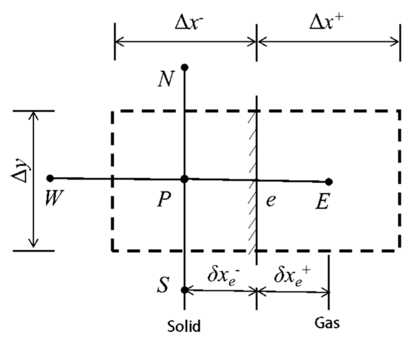
2.1.2. Governing Equation and Turbulence Model

In this paper, the software FLUENT 19.2 was used to calculate the thermal load of the cockpit and the SIMPLE algorithm based on pressure was applied. The second-order spatial discretization was adopted for the iterative calculation. The fluid was considered incompressible at a low Mach number. Thus, the governing equations at low Mach numbers referring to [11] are listed below:

Continuity equation:

$$\frac{\partial \left(\rho {\mathit{u}}_j\right)}{\partial x_j}=0$$

(1)

Momentum equation:

$$\frac{\partial \left(\rho {\mathit{u}}_i{\mathit{u}}_j\right)}{\partial x_j}=-\frac{\partial P}{\partial x_i}+\frac{\partial }{\partial x_j}\left[(\mu +{\mu }_t)(\frac{\partial {\mathit{u}}_j}{\partial x_i}+\frac{\partial {\mathit{u}}_i}{\partial x_j})\right]$$

(2)

Energy equation for fluid:

$$\frac{\partial (\rho {\mathit{u}}_{i}T)}{\partial x_i}=\frac{\partial }{\partial x_i}\left[\left(\frac{\mu }{Pr}+\frac{{\mu }_t}{P{r}_t}\right)\frac{\partial T}{\partial x_i}\right]+S_T$$

(3)

where $\rho$ is the fluid density, kg/m³; $P$ is the pressure, where $p=\rho R\mathrm{T}$ in Equation (2), Pa; μ is the dynamic viscosity, N·s/m²; $Pr$ is the Prandtl number; ${Pr}_t$ is the turbulent Prandtl number; and $S_T$ is heat source.

The RANS (Reynolds average Navier–Stokes) method provided many alternative turbulence models, such as k-ε and k-ω. The realizable k-ε model was employed in this study. This method has a good universality result. For the realizable k-ε model, an improved method was used to calculate the turbulent viscosity. The dissipation rate equation was derived from the precise transport equation for the wave vorticity. The realizable k-ε model can predict the dissipation rate distribution accurately. In addition, the realizable k-ε model can predict large pressure gradients and separation and boundary layer characteristics of the circulating airflow accurately. It can also handle the flow problems involving a rapid strain, slight rotation, and boundary layer separation more accurately. The equations are as follows [12]:

$$\frac{\partial }{\partial t}\left(\rho k\right)+\frac{\partial }{\partial x_i}\left(\rho k{u}_i\right)=\frac{\partial }{\partial x_j}\left[\left(\mu +\frac{{\mu }_t}{{\sigma }_k}\right)\frac{\partial k}{\partial x_j}\right]+G_k+G_b-\rho \epsilon -Y_M$$

(4)

$$\frac{\partial }{\partial t}\left(\rho \epsilon \right)+\frac{\partial }{\partial x_i}\left(\rho \epsilon u_i\right)=\frac{\partial }{\partial x_j}\left[\left(\mu +\frac{{\mu }_t}{{\sigma }_{\epsilon }}\right)\frac{\partial \epsilon }{\partial x_j}\right]+\rho C_{1}E\epsilon +\rho C_2\frac{{\epsilon }^2}{k+\sqrt{\upsilon \epsilon }}+C_{1\epsilon }\frac{\epsilon }{k}{C}_{3\epsilon }{G}_b$$

(5)

where A₀, C₂, ${\sigma }_k$, and ${\sigma }_{\epsilon }$ are the empirical constants, A₀ = 4, C₂ = 1.9, ${\sigma }_k=1$, ${\sigma }_{\epsilon }=1.2$; $A_S=\sqrt{6}cos\varphi$; $C_1=max(0.43,\eta /(\eta +5))$; $C_{\mu }={(A_0+A_S{U}^{*}k/\epsilon )}^{-1}$; ${\mu }_t=\rho C_{\mu }{k}^2/\epsilon$; $\eta ={(2E_{ij}\cdot E_{ij})}^{1/2}k/\epsilon$; $Eij=(\partial u_i/\partial x_j+\partial u_j/\partial x_i)/2$; ${\ddot{\Omega }}_{ij}={\Omega }_{ij}-2{\epsilon }_{ijk}{\varpi }_k$; ${\Omega }_{ij}=\overline{{\Omega }_{ij}}-{\epsilon }_{ijk}{\varpi }_k$; $\varphi =co{s}^{-1}(\sqrt{6}W)/3$; $W=E_{ij}{E}_{jk}{E}_{ki}/{(E_{ij}{E}_{ij})}^{1/2}$.

2.1.3. Radiation Model

The Do model is adopted to calculate the radiation thermal load. In the Do radiation model, the radiation transfer equation of the radiation intensity $I_{\lambda }(\mathit{r},\mathit{s})$ at $r$ along the $s^{\text{'}}$ direction is as follows [13]:

$$\nabla \left(I_{\lambda }\left(\mathit{r},\mathit{s}\right)\mathit{s}\text{'}\right)+\left(\alpha +{\alpha }_s\right)I\left(\mathit{r},\mathit{s}\right)=\alpha n^2\frac{\sigma T^4}{\pi }+\frac{{\sigma }_s}{4\pi }{\displaystyle \underset{0}{\overset{4\pi }{\int }}I\left(\mathit{r},\mathit{s}\right)\Phi \left(\mathit{s},\mathit{s}\text{'}\right)}\mathrm{d}\Omega$$

(6)

where $r$ is the position vector, ${\mathit{s}}^{\text{'}}$ is the scattering direction, n is the refraction coefficient, and T is the local temperature, K; α is absorption coefficient; ${\alpha }_s$ is scattering coefficient; σ is the Boltzmann constant, σ = 5.67 × 10⁻⁸ W/(m²·K⁴); I is the radiation coefficient, depending on the position and direction, Φ is the scattering phase coefficient; $\mathsf{\Omega }$ is space solid angle.

When dealing with the issues of heat conduction and convection at the interface of solid and fluid, the energy and momentum conservation equation should be satisfied in the calculation domain of fluid and solid, and the interface of fluid and solid should be satisfied [14]:

$$\rho c_p\frac{\partial T}{\partial t}=\nabla \cdot (\lambda \cdot \nabla T)$$

(7)

where t is time, s; $\lambda$ is the thermal conductivity, W/(m·K).

The temperature of the interface can only be determined in the calculation process. For solid surfaces with different temperatures in the flow field, the radiation heat transfer between the different solid surfaces should be considered. The net radiation heat transfer of the solid surface can be treated as an additional source term of the two control volumes located on both sides of the interface [14]. For the airship cockpit heat transfer studied here, the temperature of each part of the solid wall is different, so the radiation heat transfer between each part of the solid wall cannot be ignored. When dealing with this part of the radiation heat transfer, additional source terms can be introduced, and the additional source terms of the two control volumes are the net radiation heat transfer obtained from different walls. The cockpit’s surface temperature can be obtained by the following method:

For the air side control volume, we have:

$$S_{c,ad}=\frac{q_r\frac{(\delta x)e^{-}}{k_E}}{\frac{(\delta x)e^{-}}{k_P}+\frac{(\delta x)e^{+}}{k_E}}\cdot \frac{1}{\Delta x^{+}}$$

(8)

For the control volume located in the solid region, we have:

$$S_{c,ad}=\frac{q_r\frac{(\delta x)e^{+}}{k_E}}{\frac{(\delta x)e^{-}}{k_P}+\frac{(\delta x)e^{+}}{k_E}}\cdot \frac{1}{\Delta x^{-}}$$

(9)

where $q_r$ is the radiant heat transfer of the surface, W.

The temperature of the coupling interface is needed to calculate the $q_r$ of each surface. As shown in Figure 1, it is the schematic diagram of the gas–solid coupling interface. It can be obtained from the continuity theorem of heat flow:

$$T_e=\frac{T_p{\lambda }_p/{(\delta x)}_e^{-}+T_E{\lambda }_E/{(\delta x)}_e^{+}-q_r}{k_P/{(\delta x)}_e^{-}+k_E/{(\delta x)}_e^{+}}$$

(10)

where T_e is the temperature of the coupling interface, K.

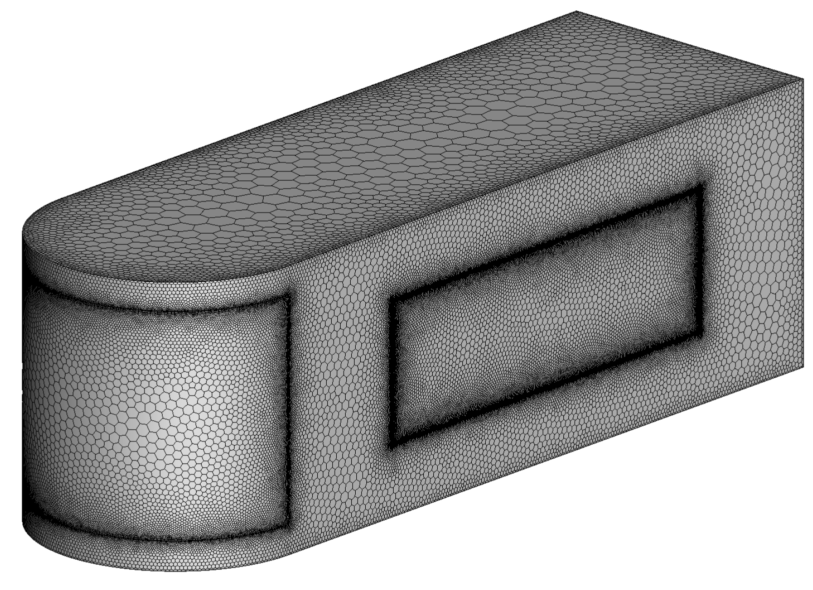
2.2. Models and Grids

A simplified geometric model for numerical simulation was established. The dimensions of the cockpit are 6 m (length) × 2 m (width) × 2 m (height) and the dimensions of the external flow field are 66 m (length) × 42 m (width) × 27 m (height). The area of the windshield and the observation window are 5 m² and 3 m², respectively. The airbag could have a significant effect on shading of the solar irradiation. In this study, the influence of the airbag was ignored. Although the assumption could lead to an overestimation of the calculated temperature, it can considerably save computing costs and obtain the primary and secondary factors affecting the total thermal loads quickly. Fiberglass, PVC foam, etc., were used in the cockpit, and the physical parameters of the main material are shown in

Table 1. Physical parameters of the materials of the envelop enclosure.

	Thermal Conductivity (W/(m·K))	Density (kg/m3)	Specific Heat Capacity (J/kg·K)
Fiberglass	1.09	2600.00	794.20
PVC Foam	0.04	1380.00	1200.00
Inner Wall	0.11	1300.00	10.00
Roof Inner Wall	0.04	1000.00	28.00

. After simplification, the main parameters of the cockpit structure are shown in

Table 2. Average parameters of the main structure.

	Average Thermal Conductivity (W/(m·K))	Average Density (kg/m3)	Average Specific Heat Capacity(J/kg·K)
Roof	0.05	1578.79	1033.50
Bulkhead	0.06	1508.51	1031.24
Floor	0.04	1086.54	1034.55
Windshield	0.22	1180.00	200.00
Window	0.22	1180.00	200.00

.

To verify the grid independence, three different quantities of grids were used to calculate the maximum cockpit temperature (T_max) at the same cruising altitude. As can be seen from

Table 3. Grid independence verification.

Number of Cells (Million)	Tmax (K)
2.44	345.07
3.23	339.33
3.60	339.37

, the calculation results are independent in different numbers of cells. When the number of cells is 2.4 million, the T_max is 345.07 K, but when the number of cells increases to 3.23 million, the T_max decreases to 339.33 K, and when the number of cells continues to increase to 3.60 million, the changes in T_max are not obvious. In order to save computing costs, the grid with 3.23 million cells was selected to carry out the following study.

As shown in Figure 2, the model was divided into unstructured hexahedron grids. Because the thicknesses of the observation window and windshield are small, it is difficult to generate grid cells. In order to improve the mesh quality and the calculation accuracy, the grid elements of the observation window and the windshield were refined. The details are shown in Figure 3. Figure 3a shows the details of the surface mesh for the observation window; the maximum size is 3.23 × 10⁻³ m², and the minimum size is 5.06 × 10⁻⁷ m². Figure 3b shows the details of the surface mesh for the windshield; the maximum size is 7.05 × 10⁻³ m², and the minimum size is 4.7 × 10⁻⁷ m².

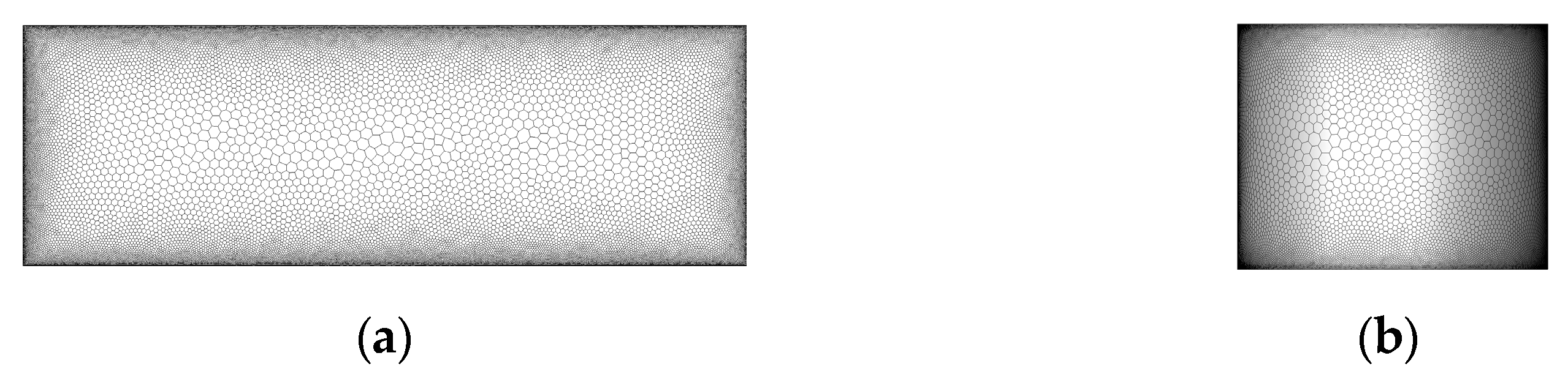
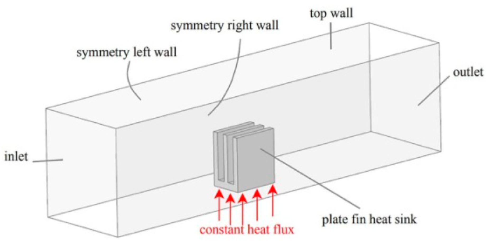
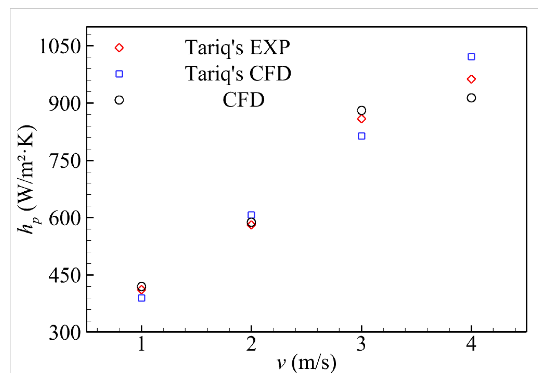
2.3. Simulation Model Verification

To validate the present simulation, this paper selected Tariq’s experiment [15] data to verify the correctness of the calculation method. Figure 4 shows the schematic diagram of the calculation model. In this model, the underside of the plate-fin sink is heated by a constant heat flux and the inlet airflow velocity is 2 m/s [15].

Inlet airflow with different free-flow velocities was calculated with a value of 2 m/s, 4 m/s, 6 m/s, 8 m/s, respectively. As shown in Figure 5, the calculated results of this paper are consistent with the experimental and simulation results of the reference. The maximum error between the calculated results of forced convection and the experimental results is 5.1% [15]. The above turbulence model and calculation method can be used to carry out the calculation work.

3. Results and Analysis

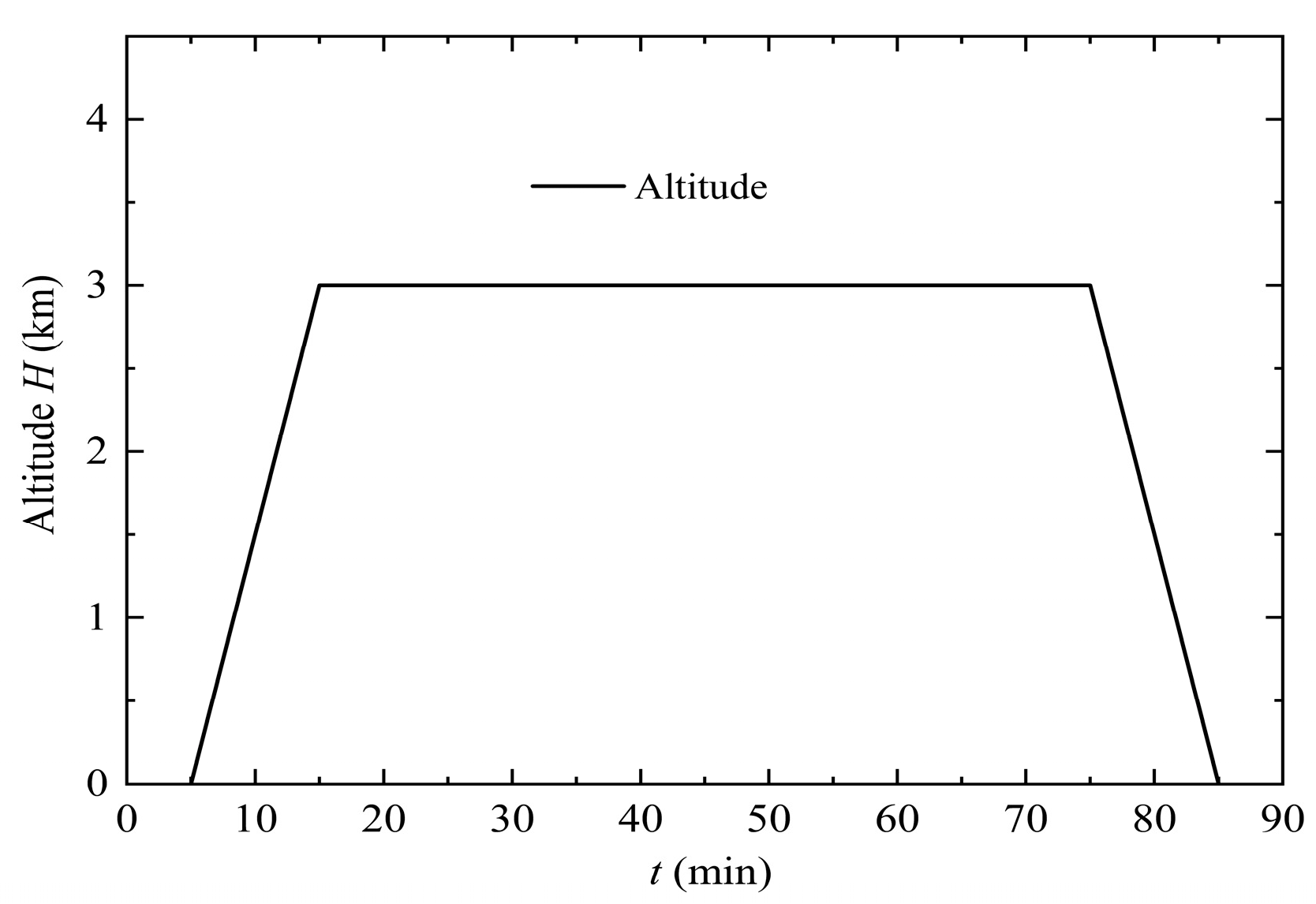
3.1. Flight Mission Envelope

The flight envelope of the airship is shown in Figure 6. Before the airship starts to take off, the cockpit reaches a stable thermal state. At t = 5 min, the airship takes off and it takes 10 min to climb from the ground to the cruise altitude of 3000 m at a constant velocity. Then, the airship cruises at that altitude for one hour. The last 10 min are spent on landing on the ground.

3.2. Results and Discussion

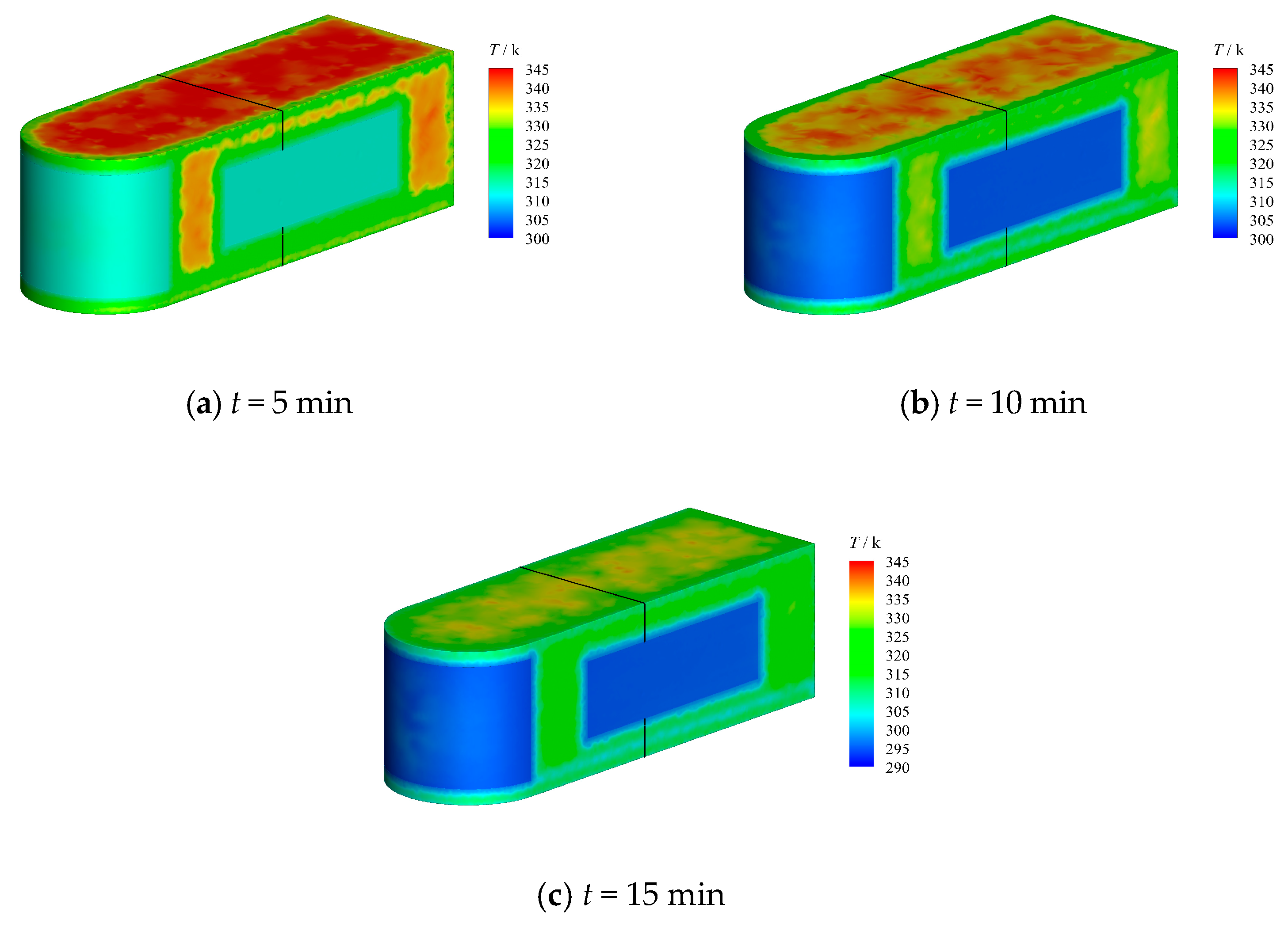
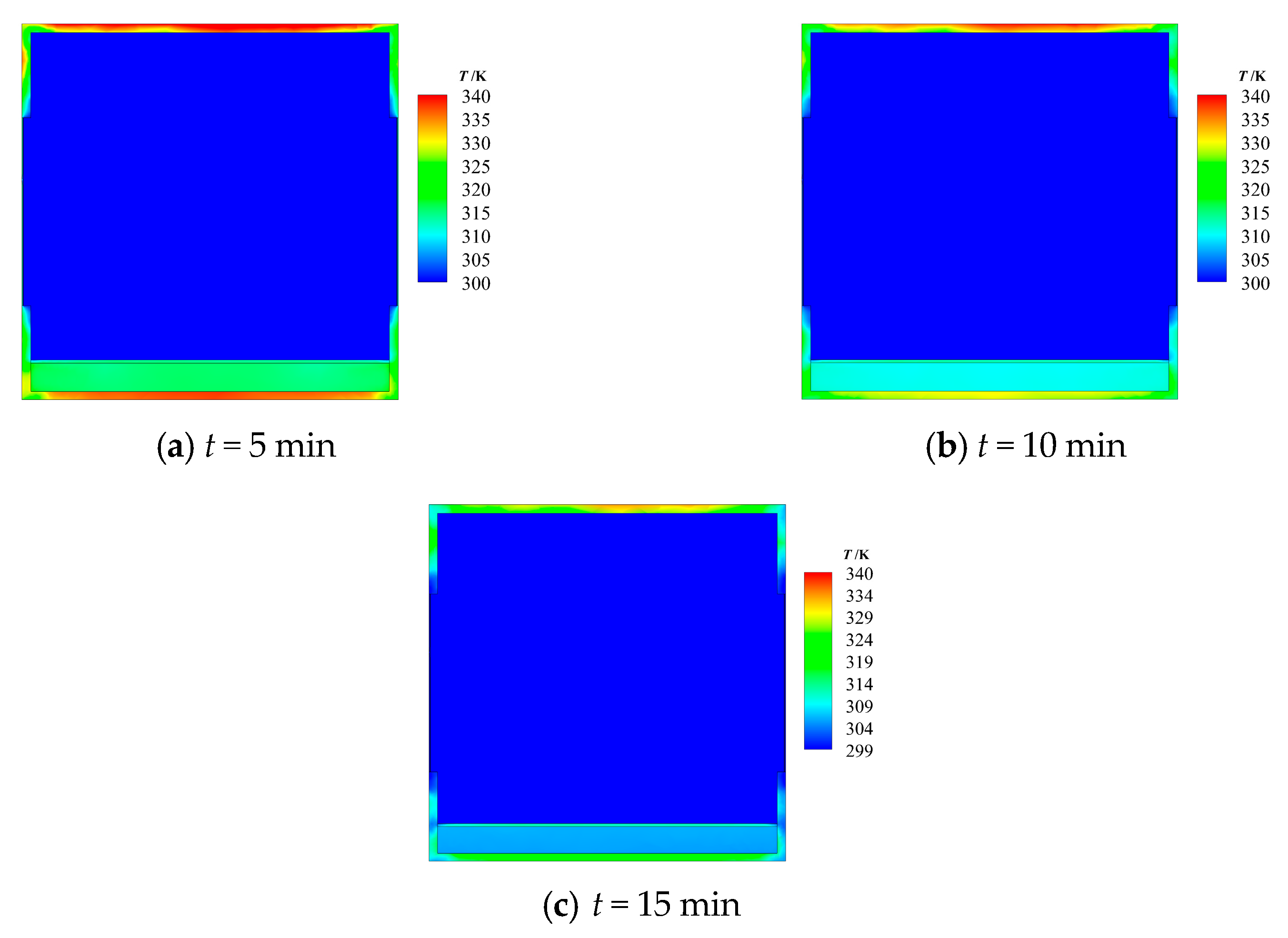
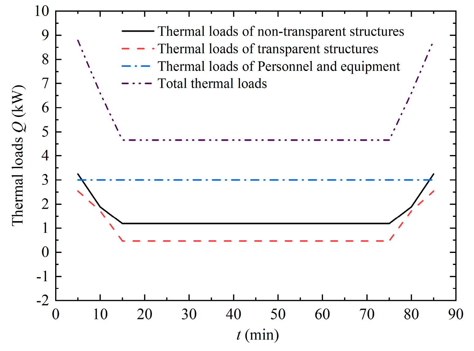
3.2.1. The Influence of Altitudes

In this section, the influences of different altitudes on the cockpit thermal loads were studied. The free-flow velocity is 40 m/s and the time is 8:00 a.m., the ground temperature is 313 K, and the temperature at cruising altitude is 293.5 K. Figure 7a shows the temperature distribution of the cockpit when the airship takes off at t = 5 min; Figure 7b shows the temperature distribution of the cockpit at t = 10 min during the ascending process; Figure 7c shows the temperature distribution of the cockpit when the airship reaches the highest altitude at t = 15 min. The temperature at the top and side walls of the cockpit is higher than that of other walls. The maximum temperature of the airship decreases with time, because the environment temperature decreases when the flight altitude increases. The high reflectivity and low absorptivity of the observation window and the windshield compared with that of the walls leads to a low temperature at the outside of the windows and the windshield, which approximates the external temperature.

Figure 8a–c show the temperature distribution of the cross-sections at x = 1 m of the cockpit corresponding to the three flight states, indicated by the black lines in Figure 7. As the flight altitude increases, the long-wave radiation intensity of the ground and the temperature of the external free-flow decreases. As a result, the temperature at the bottom of the airship gradually decreases. The highest temperature occurs at the top of the cockpit because of the effect of the solar radiation.

In this paper, only the influences of different altitudes on the cockpit thermal loads were studied, ignoring the change in the solar radiation angle and radiation intensity with time during the flight envelope. Figure 9 shows the variation in thermal load within the flight envelope, and the direction of thermal loads is positive from the outside to the inside and negative from the inside to the outside. In this study, the thermal loads of personnel and equipment was regarded as a constant; its value is 3 kW. In the ascending stage from t = 5 min to t = 10 min, the increase in the flight altitude leads to a lower free-flow temperature. Thus, the temperature difference between the cockpit surface and the free-flow temperature becomes smaller, resulting in a decrease in the total thermal loads. At t = 5 min, the total thermal load reaches a maximum of 8.8 kW. At t = 15 min, the total thermal load reaches a minimum value of 4.7 kW. In the cruising stage from t = 15 min to t = 75 min, the thermal load remains unchanged because there is no change in the external environment. In the descending stage from t = 75 min to t = 85 min, the decrease in the flight altitude leads to a higher free-flow temperature, resulting in the increase in the total thermal loads of the cockpit.

3.2.2. Influence of Solar Radiation

In this section, the influence of solar radiation is examined. The airship is in the cruise stage, the flow velocity is 40 m/s, and the external temperature is 293.5 K. The variation in solar radiation at different times is shown in

Table 4. The variation in solar radiation at different times of the day.

	8:00	10:00	12:00	14:00	16:00	18:00	20:00
Direct Normal Solar Irradiation [W/m2]	371.0	425.8	439.5	430.7	388.4	216.7	0
Diffuse Solar Irradiation—vertical surface: [W/m2]	114.4	99.9	77.48	94.4	114.4	74.8	0
Diffuse Solar Irradiation—horizontal surface [W/m2]	100.5	115.4	119.2	116.7	105.3	58.7	0
Ground Reflected Solar Irradiation—vertical surface [W/m2]	50.4	84.1	98.1	88.7	58.5	15.6	0

. As can be seen from the table, the largest intensity of solar radiation occurs from 10:00 to 14:00. These data are calculated with FLUENT19.2, using the ASHRAE Fair Weather Conditions method [16].

Figure 10 shows the thermal load curves at different times of the day. As can be seen from the figure, the largest total thermal loads of the cockpit occur from 10:00 to 14:00 of the day and the value is 5.5 kW, because of the highest intensity of solar radiation occurs during that time. After 14:00, as the intensity of solar radiation decreases, the thermal loads become smaller. The thermal loads reach a minimum at 20:00, and the value is 2.2 kW.

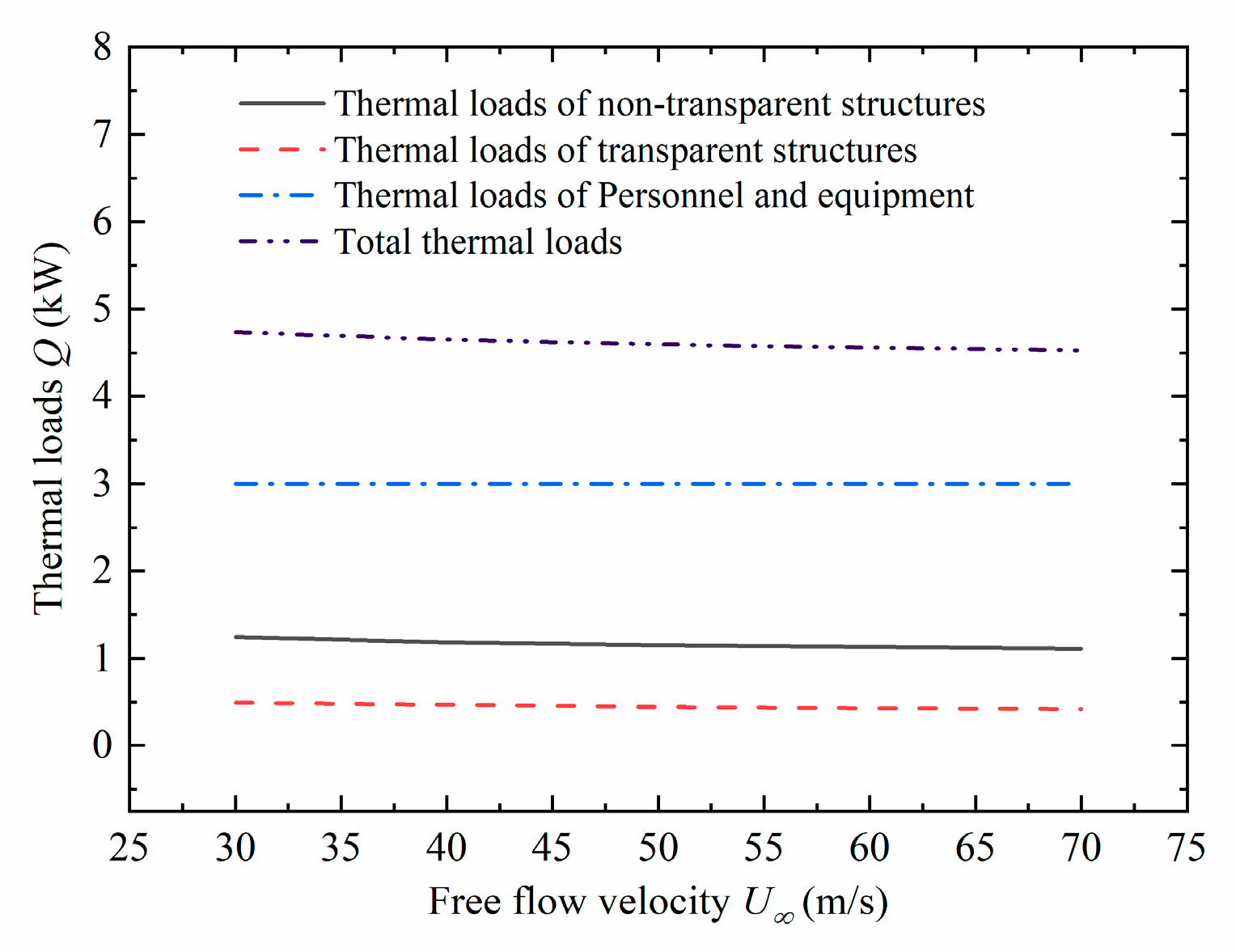
3.2.3. Influence of the Free-Flow Velocity

Here, the influence of the free-flow velocity is examined. The cockpit is in the cruising state, the time is 8:00 a.m., and the external temperature is 293.5 K. Figure 11 shows the thermal load curves with the free-flow velocity. As can be seen from the figure, the low free-flow velocity has little effect on the total thermal loads. The greater the free-flow velocity, the stronger the convective heat transfer between the free-flow temperature and the cockpit surface. Thus, the average temperature of the surface and the total thermal loads decrease when the free-flow velocity increases. Additionally, the curve in the figure decreases slowly, which shows that the free-flow velocity accounts for a relatively small change in the total thermal loads of the cockpit.

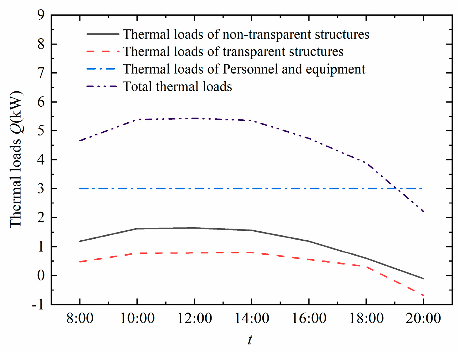
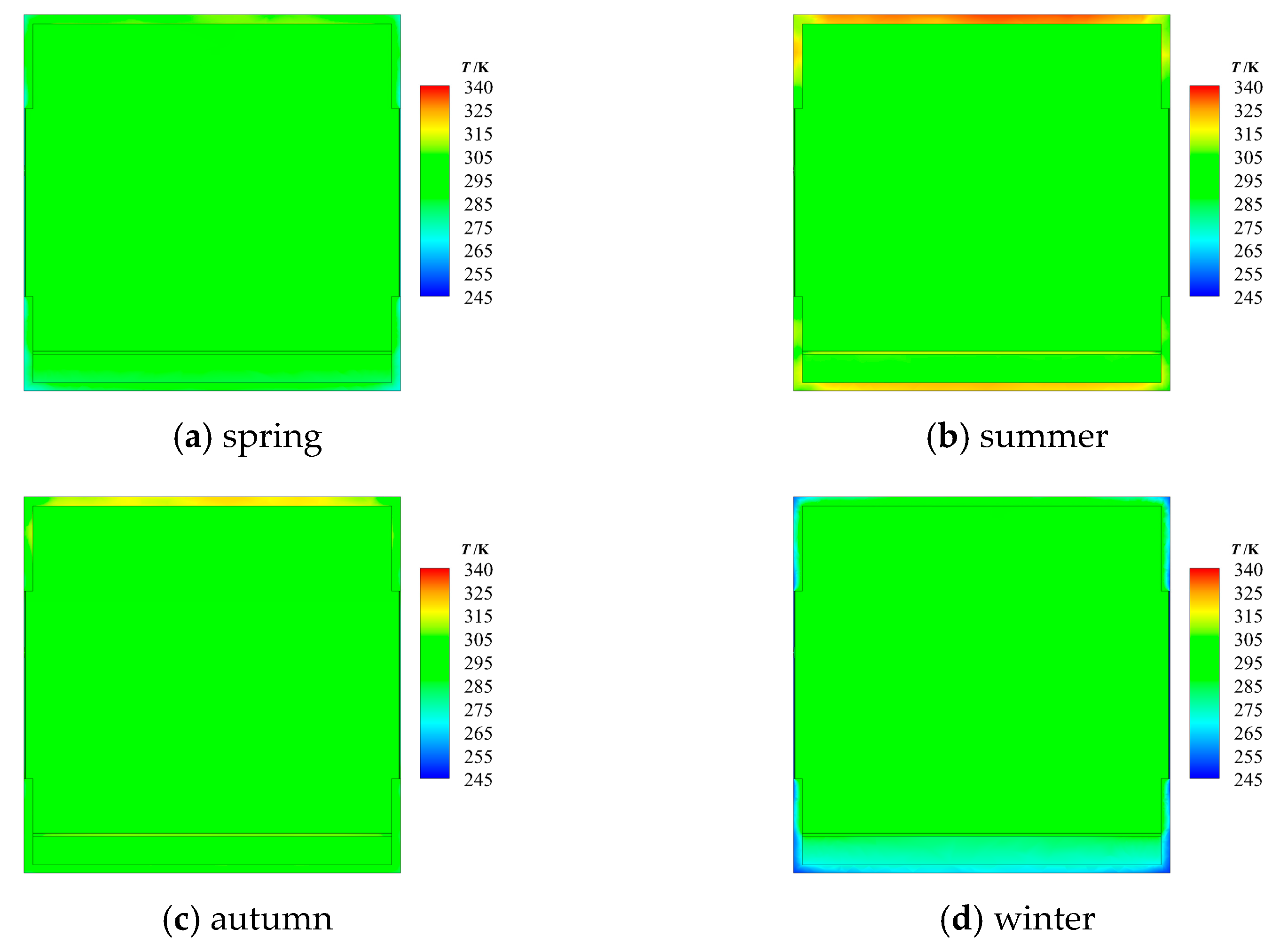
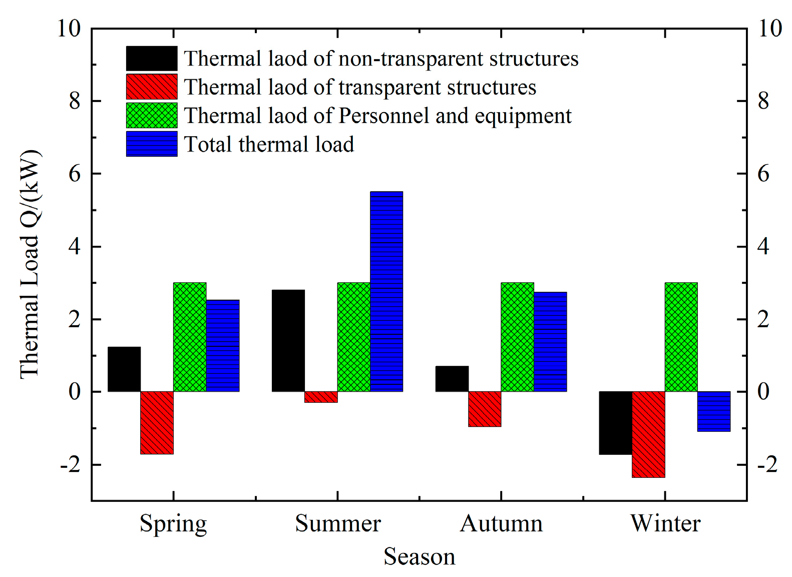
3.2.4. Influence of the Season

In this section, the influence of different seasons on the cockpit thermal loads is examined. Only one day in each season was selected for calculation. The free-flow velocity is 40 m/s and the time is 8:00 a.m. at the cruising stage. The external temperature is 262.7 K, 293.5 K, 273 K, and 243.7 K for spring, summer, autumn, and winter, respectively.

Figure 12 shows the temperature distribution of the cockpit in different seasons at the cruising stage. As shown in Figure 12a–d, the maximum temperatures in these four seasons are 311.94 K, 339.34 K, 324.67 K, 301.1 K, respectively, and it all occurs at the top of the cockpit. The difference between the maximum temperature and the minimum temperature of the cockpit across the four seasons is 38.23 K. Because of the high reflectivity and low absorptivity of the transparent structure, the temperature of it is close to that of the free-flow temperature. This phenomenon is caused by the difference in the angle of the sun, the intensity of the solar radiation, and the free-flow temperature.

Figure 13a–d show the temperature distribution of the cross-sections at x = 1 m of the cockpit in different seasons mentioned in Figure 12. At the bottom of the cockpit, the temperature is 286 K, 320 K, 296 K, 266 K, respectively. The bottom temperature of the cockpit increases first and then decreases. In summer, it reaches the maximum, and in winter, the minimum. There are two reasons for this phenomenon. Firstly, the intensity of the ground long wave radiation was affected by the intensity of the solar radiation, which influences the temperature of the cockpit bottom. Secondly, the convective heat transfer effect between the cockpit bottom and the free-flow changes when the free-flow temperature changes.

Figure 14 shows the cockpit thermal loads in different seasons. As can be seen from the figure, from spring to winter, the cockpit total thermal loads increase first and then decrease. Because of the drastic change in the external environment, the effect of season on the thermal loads is very obvious. In winter, the total thermal load is a negative value, and the heat flow direction is from inside to outside; however, in other seasons, the total thermal load is a positive value, and the heat flow direction is from outside to inside. It reaches the maximum in summer, with a value of 5.5 kW, and the minimum in winter, with a value of −1.08 kW. Therefore, the change in external conditions caused by the change in season has a great influence on the thermal loads of the cockpit.

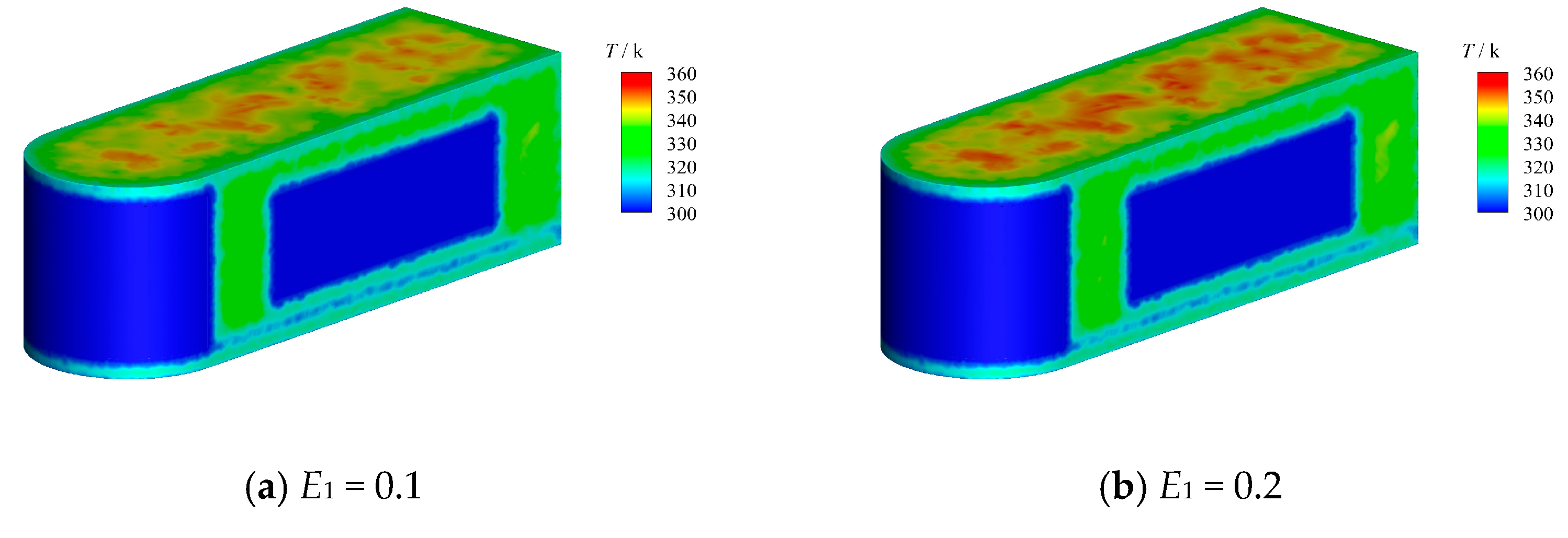
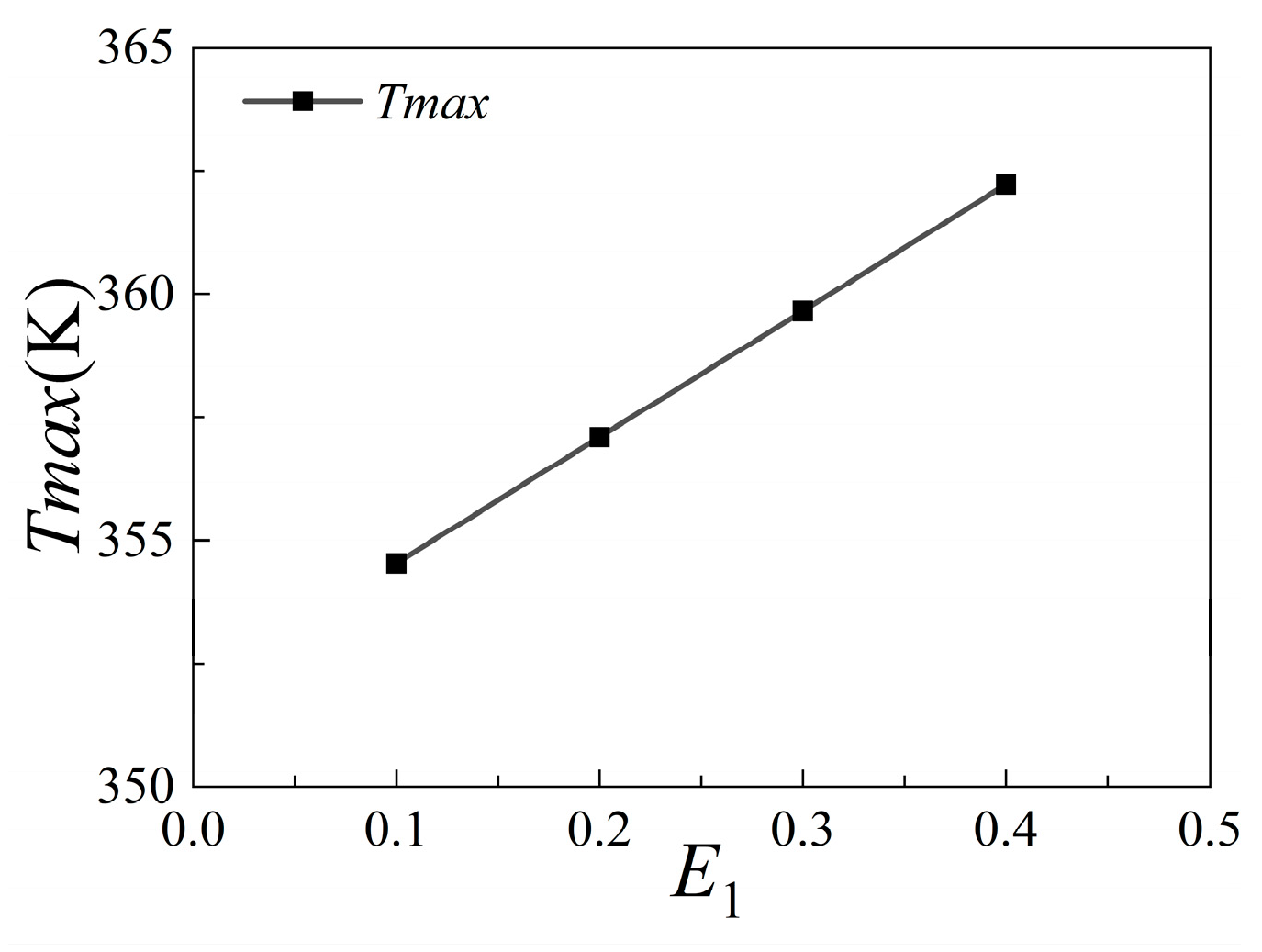
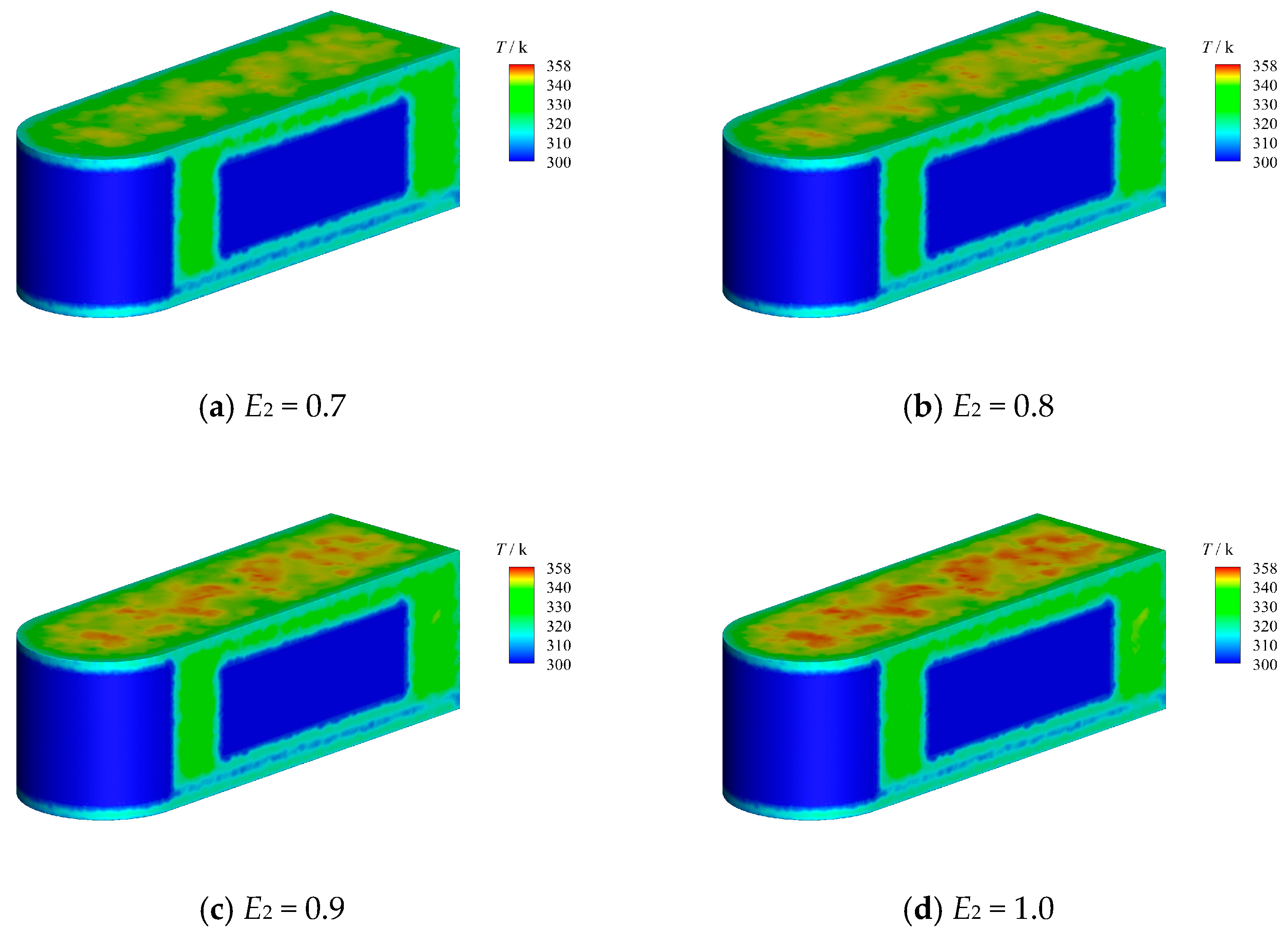
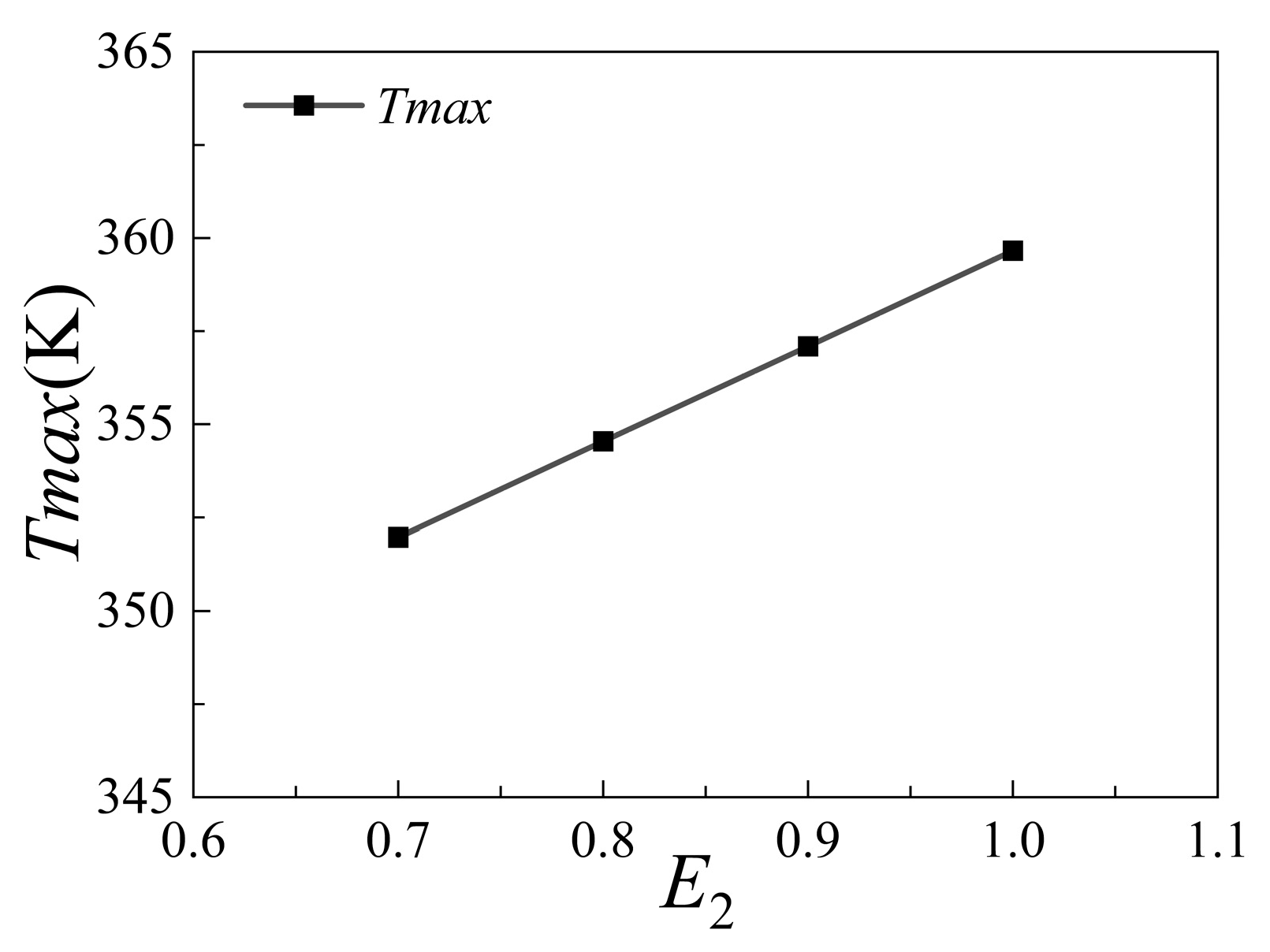
3.2.5. Influence of the Solar Absorptivity and Infrared Emissivity

In this section, the influence of solar absorptivity and infrared emissivity are examined. Here, the solar absorptivity is expressed as E₁ and it varies from 0.1 to 0.4, while the infrared emissivity is expressed as E₂ and it varies from 0.7 to 1.0. The absorptivity and emissivity of a material are a function of the electromagnetic spectrum. For the same electromagnetic spectrum, the absorptivity of a material is equal to its emissivity [17].

Figure 15 shows the temperature distribution with solar absorptivity changing from 0.1 to 0.4. The maximum temperatures all occur at the top of the cockpit. As the solar absorptivity increases, the maximum temperature of the wall also increases. Figure 16 shows that T_max varies from 354 K to 363 K when E₁ varies from 0.1 to 0.4. This phenomenon shows that the cockpit’s absorption of solar radiation is greater than the emission to the environment.

Figure 17 shows the temperature distribution with infrared emissivity changing from 0.7 to 1.0. The maximum temperatures all occur at the top of the cockpit. This phenomenon is consistent with the above. Figure 18 shows that T_max varies from 352 K to 360 K when E₂ varies from 0.7 to 1.0. As the infrared emissivity increases, the temperature of cockpit surface also increases. Thus, the absorption rate has a more substantial effect than emissivity.

4. Conclusions

The thermal loads of the cockpit of a sightseeing airship and the surface temperature distribution were obtained in this paper. The influences of different times of the day, flight altitudes, seasons, and thermal radiation properties of the cockpit surface material were investigated. The results show that solar radiation has a great influence on the cockpit transient thermal loads. As the flight altitude increases, the thermal loads decrease from 8.8 kW (H = 0 m) to 4.7 kW (H = 3000 m). The total thermal loads of an airship decrease gradually with the increase in altitude due to decreased ambient temperature. Because of the change in solar radiation intensity and solar radiation angle, the thermal loads increase greatly, from 2.2 kW (8:00 a.m.) to 5.4 kW (12:00 a.m.). The influence of the free-flow velocity is not very obvious at an altitude of 3000 m, as discussed here. The total thermal loads of the airship decrease as the surrounding free-flow velocity increases. Additionally, the impact of the free-flow velocity on non-transparent structures is more pronounced than that on transparent structures. The influence of the free-flow velocity on the thermal loads is relatively small. Thermal loads of the cockpit changed obviously under different seasons. Additionally, the solar absorptivity of the cockpit surface material has a more substantial effect than the infrared emissivity on the temperature of the cockpit. This study provides a comprehensive assessment of external factors impacting the cockpit, offering a reference for the design of environmental control systems for airship cockpits.

References

1. Jian, X.; Li, N. Research on the Calculation Method of Transient Heat Load for Aircraft Cabin. Civ. Aircr. Des. Res. 2010, 3, 30–33. [Google Scholar]
2. Shou, R.; He, H. Aircraft Environment Control; Beijing University of Aeronautics and Astronautics Press: Beijing, China, 2004; pp. 1–5. [Google Scholar]
3. Hu, S. Calculation of Helicopter Cabin Thermal Conductivity. Helicopter Technol. 2017, 1, 36–38. [Google Scholar]
4. Wang, L.; Zhao, J.Q. Numerical Simulation of Heat Transfer in Aircraft Cabins. Comput. Simul. 2008, 5, 44–46+142. [Google Scholar]
5. Fan, W.; Zhuang, D.; Yuan, X.; Li, D. Calculation and Simulation of Transient Heat Load for Cabins. J. Beijing Univ. Aeronaut. Astronaut. 2001, 27, 654–657. [Google Scholar]
6. Zhang, X.; Yang, C.; Yuan, X. Engineering estimation methods of thermal load of airplane. J. Beijing Univ. Aeronaut. Astronaut. 2009, 35, 1503–1506. [Google Scholar]
7. Liu, Z.; Dong, S.; Zhou, Y.Y.; Zhang, S.; Fu, Y. Parameter Identification and Simulation Method of 2-Node Thermal Network Model of Aircraft Cabin. IET Conf. Proc. 2022, 7, 151–156. [Google Scholar]
8. Rezanova, E.A.; Merkulovb, V.I.; Rossovac, K.V.; Tishchenko, I.V. The Comparative Analysis of External Heat Transfer Calculation Methods for a Solar Aircraft Spacesui. MATEC Web Conf. 2020, 324, 03007–03009. [Google Scholar] [CrossRef]
9. Wu, J.; Jiang, F.; Song, H.; Liu, C.; Lu, B. Analysis and validation of transient thermal model for automobile cabin. Appl. Therm. Eng. 2017, 122, 91–102. [Google Scholar] [CrossRef]
10. Omle, I.; Kovács, E.; Bolló, B. Applying recent efficient numerical methods for long-term simulations of heat transfer in walls to optimize thermal insulation. Results Eng. 2023, 20, 101476. [Google Scholar] [CrossRef]
11. Frank, P.I.; David, P.D. Introduction to Heat Transfer, 3rd ed.; John Wiley and Sons: Hoboken, NJ, USA, 1996. [Google Scholar]
12. Shaheed, R.; Mohammadian, A.; Gildeh, H.K. A comparison of standard k–ε and realizable k–ε turbulence models in curved and confluent channels. Environ. Fluid Mech. 2019, 19, 543–568. [Google Scholar] [CrossRef]
13. Yang, S.; Tao, W. Heat Transfer; Higher Education Press: Beijing, China, 2019. [Google Scholar]
14. Tao, W. Numerical Heat Transfer; Xi’an Jiaotong University Press: Xi’an, China, 2001. [Google Scholar]
15. Tariq, A.; Altaf, K.; Ahmad, S.W.; Hussain, G.; Ratlamwala, T.A.H. Comparative numerical and experimental analysis of thermal and hydraulic performance of improved plate fin heat sinks. Appl. Therm. Eng. 2021, 182, 115949. [Google Scholar] [CrossRef]
16. ANSYS® Fluent 19.2, Release 19.0, Help System, ANSYS Fluent User’s Guide, ANSYS, Inc. 2018. Available online: https://pdfcoffee.com/ansys-fluent-tutorial-guide-2019-pdf-free.html (accessed on 3 December 2023).
17. Yang, S.; Tao, W. Heat Transfer Science; Higher Education Press: Beijing, China, 2019. [Google Scholar]
Figure 1. Schematic diagram of gas–solid coupling interface.
Aerospace 11 00127 g001
Figure 2. The surface mesh of the cockpit.
Aerospace 11 00127 g002
Figure 3. The details of the surface mesh for (a) the observation window, (b) the windshield.
Aerospace 11 00127 g003
Figure 4. Schematic diagram of the calculation model [15].
Aerospace 11 00127 g004
Figure 5. Results of forced convection verification.
Aerospace 11 00127 g005
Figure 6. Flight envelope of the airship.
Aerospace 11 00127 g006
Figure 7. Temperature distribution of the cockpit at different flight stages.
Aerospace 11 00127 g007
Figure 8. Temperature distribution of cockpit section in x = 1 m at different times.
Aerospace 11 00127 g008
Figure 9. Cockpit transient thermal load.
Aerospace 11 00127 g009
Figure 10. Cockpit thermal loads at different times of the day.
Aerospace 11 00127 g010
Figure 11. Cockpit thermal loads at different free-flow velocities.
Aerospace 11 00127 g011
Figure 12. Temperature distribution in different seasons.
Aerospace 11 00127 g012
Figure 13. Temperature distribution of cockpit section at x = 1 in different seasons.
Aerospace 11 00127 g013
Figure 14. Cockpit thermal load in different seasons.
Aerospace 11 00127 g014
Figure 15. Temperature distribution with different solar absorptivity.
Aerospace 11 00127 g015aAerospace 11 00127 g015b
Figure 16. Effect of solar absorptivity on Tmax.
Aerospace 11 00127 g016
Figure 17. Temperature distribution of four infrared emissivity values.
Aerospace 11 00127 g017
Figure 18. The Tmax changes with infrared emissivity.
Aerospace 11 00127 g018