Abstract
A multisubstructure-based method for assessing the deformation and stress of a fine-meshed model according to a coarse model was proposed. Integrating boundary conditions in a local fine-meshed model, a displacement mapping matrix from the coarse model to the fine-meshed model was constructed. The method was verified by a three-level panel in a fluid–structure interaction (FSI) framework by integrating the steady vortex lattice method (VLM). A comparison between the inner deformation distribution of the coarse model and that of the global fine-meshed model obtained from MSC.Nastran was carried out, and the results showed that the coarse model failed to demonstrate reliable strains and stresses. In contrast, the proposed method in this paper can effectively depict the inner deformation and critical stress distribution. The deformation error was lower than 8%, meeting engineering requirements. Moreover, the results of different working conditions can achieve a similar relative error of displacement for an identical position. The easy storage of the displacement mapping matrix and the convenience of the boundary information transformation among all substructure levels are prominent aspects. As a result, there is a solid foundation for addressing the time-dependent problem in spite of the simultaneity and region.
1. Introduction
A variety of aeroelasticity phenomena, such as the flutter margin, static and dynamic loads, and structure stress, need to be taken into consideration in aircraft structure design. An initial structure using a finite element model (FE model) that meets basic stress and buckling requirements under a series of preliminary design load conditions was constructed during a preliminary design process. The lowest-fidelity model was utilized for the aeroelastic design and analysis in several iterations [1,2]. However, this meant that, on the one hand, the model of the structure could not be updated in real time and, on the other hand, it failed to provide adequate and accurate information for designers in predicting performance [3]. In addition, the literature indicates that a reduced-order structure model can be used to balance the efficiency and precision of the aeroelastic calculations, while a full-order structure FE model is imperative for strength analysis [1]. Confronted with the structure design of flight vehicles, the different focuses on aeroelasticity and structure strength imply further integration reinforcement for multiple disciplines in order to consider how structure strength can be obtained through a rational strength design. Currently, many researchers are investigating the application of multiple discipline optimization (MDO) in flight vehicle design with respect to model order reduction and design efficiency improvements through the integration of multiple disciplines [4]. In an MDO framework, Livne et al. [5] applied the equivalent plate approach to assess specific effects, whereas ignorance of the actual structure and the FE model resulted in a failure to provide stress details. Bindolino et al. [6] identified displacement with satisfactory accuracy based on the perturbation mode approach [7], but their model was still deficient in the accuracy of its strain and stress analyses. Accordingly, MDO focuses limited attention on the stress of the structure during the preliminary design process; moreover, the reduced-order structure model fails to depict the stress of the structure with respect to both geometry and timescales. Specifically, MDO is carried out in three stages (conceptual, preliminary, and detailed) during the aircraft design process, with the result that long-term monitoring of the structure is not supported. For the MDO framework, aeroelasticity is evidently a factor, which can introduce radical impacts on the design of the structure [3,8,9,10]. In addition, aeroelasticity is a real scenario that aircrafts encounter. Therefore, stress analyses should take aeroelasticity into consideration. However, due to the lack of investigation regarding the aeroelasticity output with respect to the structure [11], it is necessary to build an aerodynamic structure framework embedding a multisubstructure-based mapping method, which is based on the geometric multiscale finite element method (GMsFEM) [12] and the dynamic substructure method to describe the displacement and stress of structures influenced by aerodynamic loads.
The dynamic substructure method is divided into a fixed-interface substructure class and a free-interface substructure class [13]. For the former class, the integration of the interface’s displacement and the constraint mode set is used to depict the implicated movement, and the free vibration mode set with all restrained boundaries (that is, the fixed-interface main mode set) is regarded as the basis for describing the relative movement [14,15]. The distinction between these two substructure classes lies in the main mode set with different displacement boundary settings. For the fixed-interface substructure class, the fixed-interface main mode set is obtained with a fixed boundary, whereas all the interface physical degrees of freedom are set free for the substructure modal analyses with respect to a free-interface substructure. The free boundary modal set for the free-interface substructure requires a balance between precision and the number of modal bases. The modal basis set requires supplementation due to the neglecting effect of adjacent substructures [16] and the truncation of higher-order modes [17,18,19,20]. Based on the comparison of different substructure classes, the fixed-interface substructure class is considered, due to having less of a modal basis and relatively reliable precision.
There exists an analog between the substructure and the element in the finite element method (FEM). The shape function set is composed of a nodal-based shape function, an edge-based shape function, and a face-based shape function in the higher-order FEM [21]. Furthermore, the constraint mode set resembles the nodal-based shape function, and the fixed-interface main mode set resembles the face-based shape function. Naturally, the displacement in the interface can be realized by combining the displacement of known grids with the edge-based shape function. Zander et al. [22] investigated the multi-level element method, by discretizing proportionally and reconstructing the element shape function. This method revealed an efficiency problem due to the reproduction of the element shape functions. However, the substructure method is based on the component level and not the element level, which means that this technology may be capable of overcoming this efficiency problem.
The dynamic substructure method is widely used in aeroelasticity analysis for structural order reduction while possessing similar properties to the FE; it can bridge the research gap in analyzing aeroelasticity and structure strength for both preliminary design and long-term structure monitoring. Higher-order modes are required in order to seize detailed physical information for describing the displacement and stress of delicate positions. The proposed multisubstructure-based displacement mapping can create a hierarchy for the target positions to capture detailed data on their displacement using relatively fewer degrees of freedom globally. The proposed mapping method can transfer the influence of the last coarse-mesh substructure to the current fine-mesh substructure through displacement boundary, thus facilitating independent analysis among different meshed substructures, which is a distinct advantage.
This paper is structured as follows. In Section 1, the theoretical method used for the proposed structure mapping and aerodynamic modelling is introduced. In Section 2, an aerodynamic model and a three-level panel FE model are established to verify the proposed method and build an aerodynamic structure analysis framework. The results are analyzed and discussed in Section 3. Conclusions are drawn in Section 4.
2. Methodology
Due to the previously discussed advantages, the proposed mapping method is based on a multi-level substructure, with the deduction based on a fixed-interface substructure method (Craig-Bampton Substructure Method, CB Method) due to its advantages. Using the CB method, the substructure’s displacement was analyzed in two parts: (1) the implicated movement determined by integrating the boundary displacement and the constraint mode set and (2) the relative movement determined by integrating the fixed-interface main mode set and its generalized coordinates. The generalized coordinates corresponding to the relative movement projected on the fixed-interface main mode basis can be solved using the principle of minimum potential energy. Additionally, boundary displacement information can even be considered as the corresponding generalized coordinates of the constraint mode set. Obviously, there is a correlation between the information deduced from the last coarse-mesh model and the unknown displacement information of the current boundary, which can normally be calculated using the edge-based shape function at the FE level. However, a thin panel spline (TPS) can also satisfy the correlation at the component level, which is also a widely used method for the information transition of the fluid–structure interface. The steady vortex lattice method (VLM) was used to perform aerodynamic modeling so that the proposed method can be studied in a fluid–structure interaction (FSI) framework.
2.1. Craig-Bampton Substructure Method
The undamped substructure dynamic equation is as follows:
where is the physical mass matrix, is the physical stiffness matrix, is the physical displacement vector, and f is the load vector.
Substructure displacement is divided into two parts: (1) the displacement vector of substructure inner grids, and (2) the displacement vector of substructure boundary grids:
According to ref. [13], a complete mode set is composed of a constraint mode set and a fixed-interface main mode set . The former one involves an implicit movement that transfers the influence of adjacent substructures to the substructure under analysis by inducing displacement boundary conditions, while the latter one allows us to determine deformation based on implicit coordinates. Therefore, is a series of substructure shape modes of interior freedoms resulting from unit displacement of every single boundary freedom while all other boundary freedoms are completely constrained. denotes the free vibration mass-normalized modes with all boundaries constrained. Both mode sets are solved using Equation (3).
Accordingly, is satisfied as follows:
where is an identity matrix and , and is the eigenvalue in Equation (3).
Eventually, the substructure displacement is obtained using Equation (5).
where is the generalized coordinate vector corresponding to the fixed-interface main mode set .
2.2. Displacement Mapping under Inconformity Interface
In this section, a static displacement mapping is carried out by integrating the principle of minimum potential energy and the CB method.
- (1)
- Displacement Recursion
Here, attention is focused on the displacement achievement of the fine-mesh model using the displacement information of the coarse model. The -level substructure is defined to be finer than .
It is assumed that the boundary displacement of the -level substructure is as follows:
where is the boundary displacement of the -level substructure, is the interpolation matrix, and is the displacement of the -level substructure.
Substituting Equation (6) into Equation (5), the displacement relationship between the - and -level substructures can be written as follows:
where .
Iterating the recursion of Equation (7) to the first-level substructure, the displacement relationship between the -level and the first-level substructures is determined as follows:
where , and .
is the constraint mode set projection of all substructure levels at the level. is a combination of fixed-interface main mode sets at all levels that describe the inner deformation of the -level substructure. is a generalized coordinate vector that corresponds to the fixed-interface main mode sets of all substructure levels. In particular, the existence of is because the constraint mode set is linearly independent, corresponding to the fixed-interface mode set, but it is not normalized. Equation (8) demonstrates that higher displacement accuracy can be achieved in fine models via local hierarchy.
- (2)
- Generalized Coordinate Solution
The potential energy functional of the -level substructure in a discrete form is determined as follows:
where , , , and is the load vector of the -level substructure. and denote a generalized stiffness matrix corresponding to the constraint mode and a generalized stiffness matrix corresponding to the fixed-interface main mode, respectively. is the generalized stiffness matrix of the constraint mode and the fixed-interface main mode due to the non-orthogonality.
The variation about in Equation (9) is as follows:
According to the principle of minimal potential energy, the solution in Equation (10) is equal to zero, and the generalized coordinates corresponding to the value of the -level substructure are determined as follows:
Substituting Equation (11) into Equation (8), the generalized coordinate vector can be expressed as follows:
where and are the generalized flexibility matrix and the generalized force vector of all former substructure levels, respectively.
where denotes the boundary generalized force of all former substructure levels projecting on the fixed-interface main mode set of every level substructure. Substituting Equation (6) into Equation (13), Equation (8) can be written as follows:
where denotes the boundary conformity condition among every level substructure, called the generalized displacement conformity condition, and denotes a displacement vector of all former -level substructures.
2.3. Interpolation Theory
The generalized displacement conformity condition in Equation (14) is used to depict the boundary displacement of this level using the information of the former level, which comprises a series of shape functions. In higher-order FEM, the displacement of hanging nodes is described by the integration of nodal-based shape functions and edge-based shape functions. However, the shape function sets are based on the element level, which may result in numerical and efficiency problems [23,24]. Accordingly, the TPS [25] is utilized to address hanging node information at the component level to avoid defects of the higher-order FEM.
Assuming known vectors in the -dimensional space, these vectors are related to multiple functions , which are vectors in an -dimensional space. Modeling the infinite plate spline (IPS) for every component in , the equation can be written as follows:
Thus, the interpolation matrix can be written as follows:
where =, , , and is a parameter for precisely passing the known grids. Eventually, the interpolated information is derived using the following equation:
where , , .
Therefore, in Equation (6) can be written as .
Regarding the load transfer from aerodynamic forces to the structure, the aerodynamic force acting on the structure can be determined by integrating the principle of imaginary work and TPS. Assuming the virtual displacement of the structure model , the virtual displacement of the aerodynamic model , the aerodynamic force acting on the aerodynamic model , and the equivalent force acting on the structure , the relationship among the four quantities satisfies the following equation:
Substituting Equation (17) into Equation (18), is determined as follows:
2.4. Aerodynamic Modeling
In this study, aerodynamic modeling is based on a steady VLM [26]. In the flow field, the integral of the flow speed along a closed curve is defined as circulation, which is expressed as follows:
where is the flow velocity vector in three dimensions, and is a closed curve. A potential function exists that is independent of the integral path in the irrotational flow field, and its differential relative to the coordinates is a function of the fluid velocity:
Moreover, the Laplace function in a low-velocity incompressible flow field can be written as follows:
Equation (22) satisfies the Neumann boundary, which implies the impenetrable boundary of the object:
where and are the velocity vector and normal vector of the object’s surface, respectively.
Steady aerodynamic modeling is carried out using a combination of Equations (22) and (23), which are solved via basic solution superposition, such as the superposition of the vertex and dipole. Using the VLM, the vertex ring is chosen as the basic solution, which naturally satisfies the Kelvin condition and flow boundary conditions naturally and is arranged on aerodynamic elements. To ensure the total circulation constant, the influence of the flow field is impaired, along with the increase in distance, as described in Equation (24).
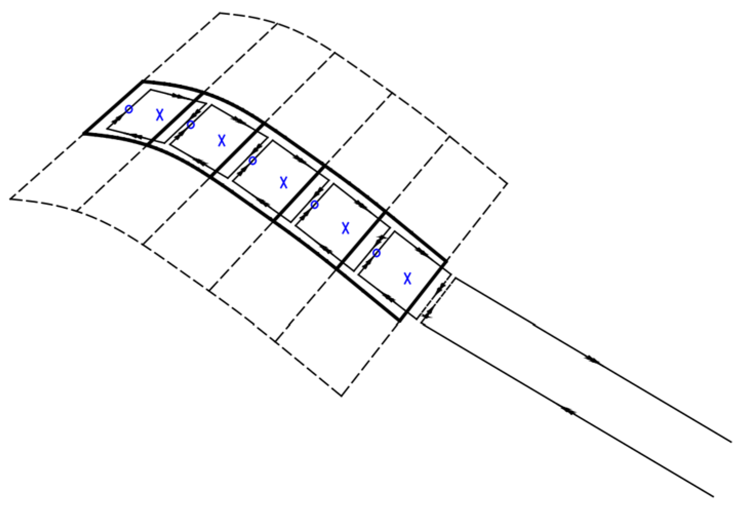
The aerodynamic surface is proportioned chordwise and spanwise into elements, where vertex rings are arranged to solve the aerodynamic loads. A vertex ring is composed of four intensity-equal end-to-end linear vertexes. The free vertex of the surface, which is parallel to the flow direction, extrudes from the tail edge, as shown in Figure 1. The aerodynamic load acts on the midpoint vertex lattice, along with a quarter of the chord line (denoted as “○”), while the control point, which is determined using Equation (23), is set on the midpoint vertex lattice, along with three-quarters of the chord line (denoted as “×”).
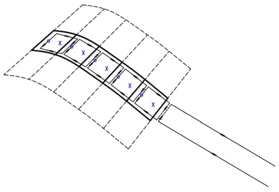
Figure 1.
Vertex ring arranged in vertex lattice [27].
3. Structural and Aerodynamic Modeling
In this section, the structural model and load cases are introduced in Section 3.1 and Section 3.2, respectively; then, the proposed method is validated through simulations in Section 3.3. For comprehensive validation, the working conditions include different load combinations outside the FSI framework and the loads inside the FSI framework.
3.1. Structural Model
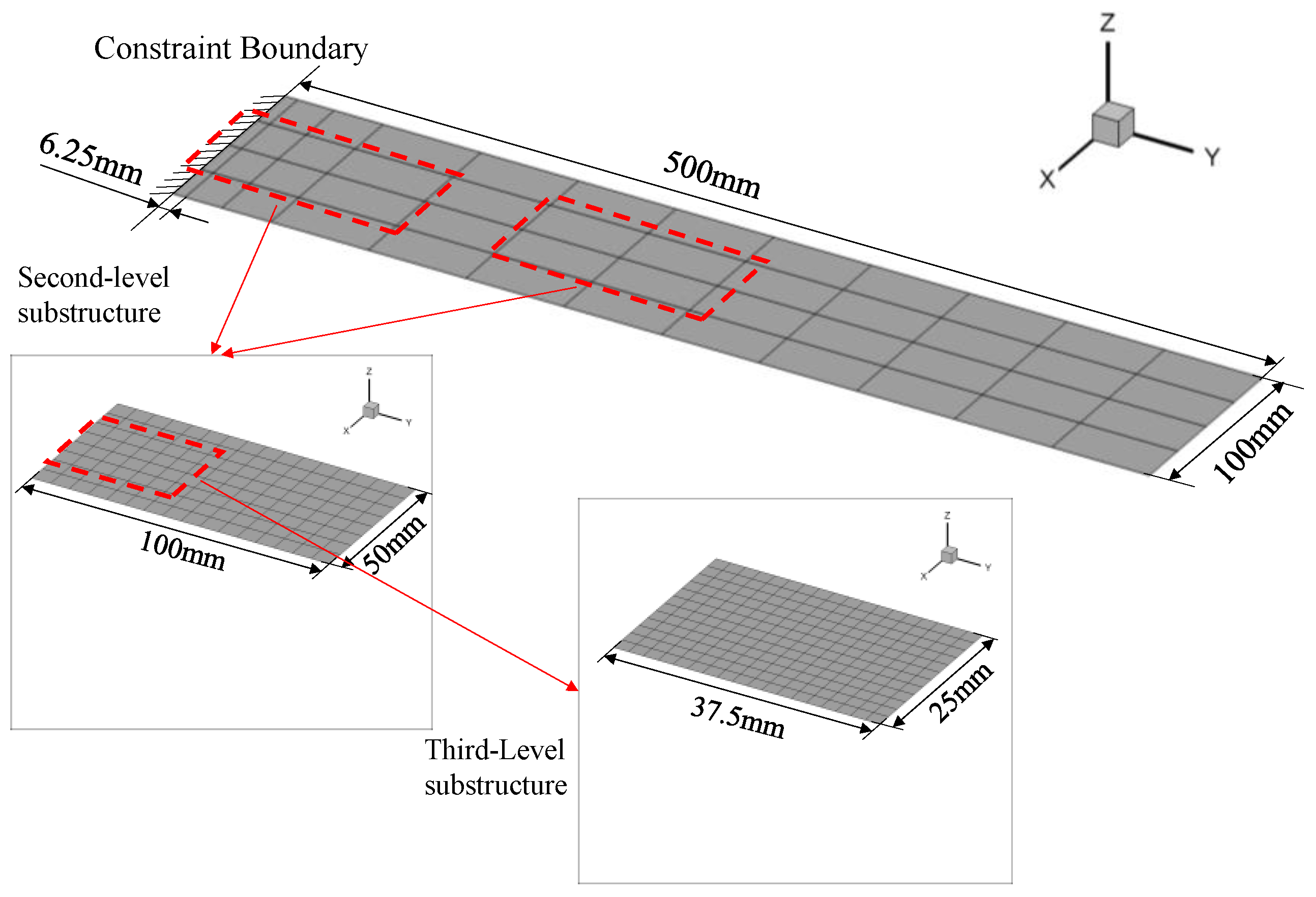
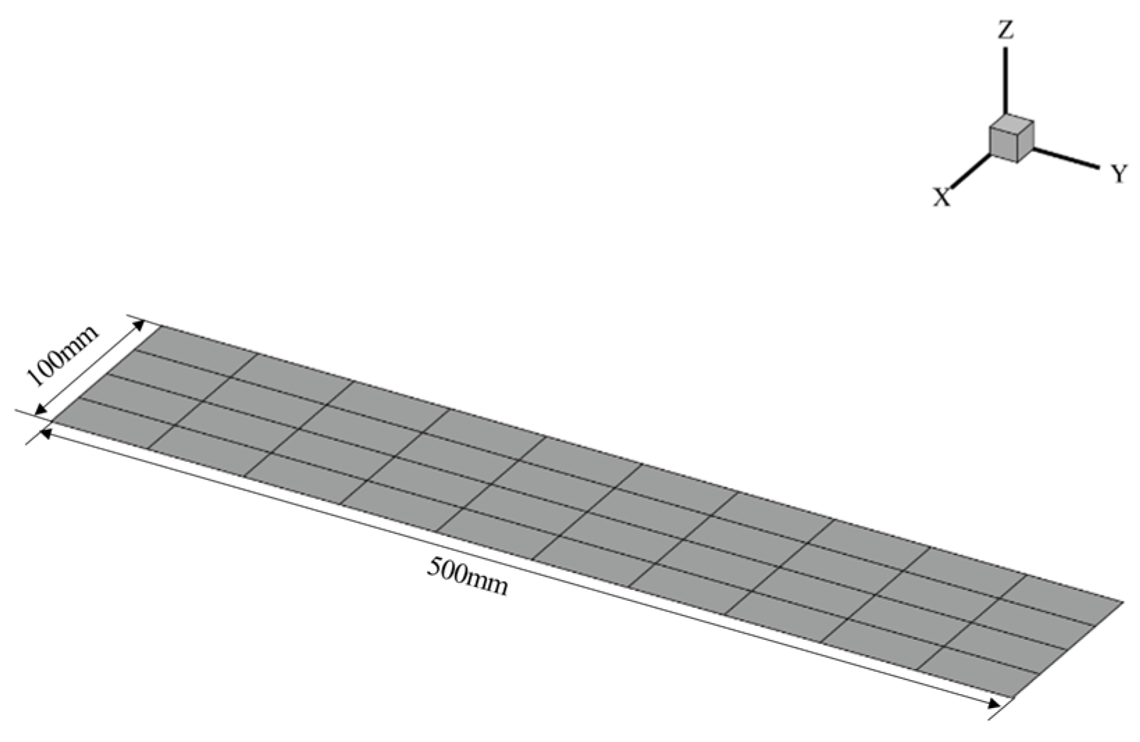
The proposed method is verified using a three-level panel, with a length of , width of , and thickness of . The material properties are listed in Table 1. The structure FE model is shown in Figure 2, where the first-level substructure denotes the entire panel with a constraint boundary on one side. Specifically, the displacement gradient around the constraint boundary is dramatically altered such that denser local elements are arranged for interpolation sampling. Second- and third-level substructures are also demonstrated in Figure 2 as well. The accuracy of the proposed method was compared with that of two FE models involving global element densities corresponding to the second- and third-level substructure, presented in Figure 3 and Figure 4.

Table 1.
Material properties.
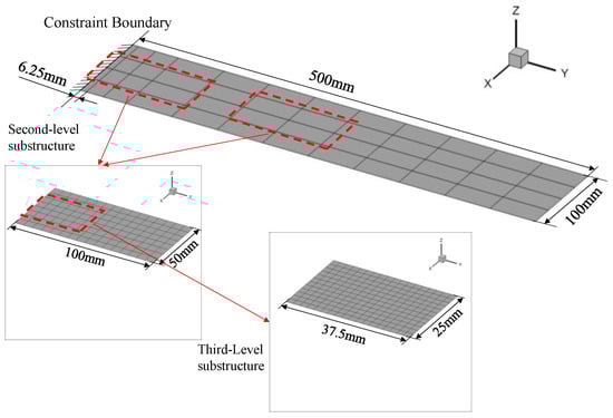
Figure 2.
Structural finite element model.
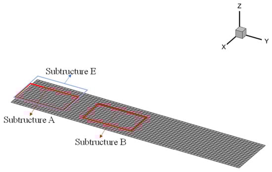
Figure 3.
Locations of second-level substructures.
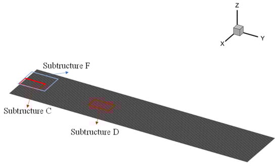
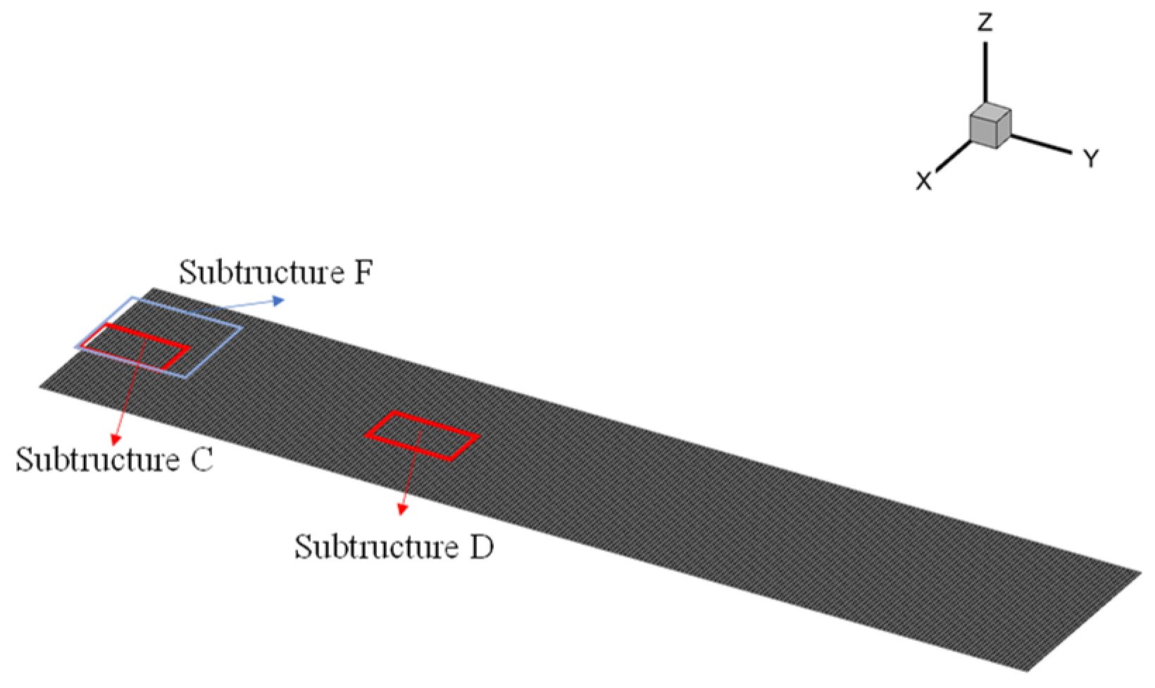
Figure 4.
Locations of third-level substructures.
3.2. Load Cases
Within the FSI framework, loads are subject to the angle of attack, airflow speed, the aerodynamic surface, etc., and these are relatively unilateral in assessments using the structural mapping method. Therefore, different load cases are taken into consideration outside and inside the FSI framework to comprehensively verify the structure mapping method.
- (1)
- Load Cases Outside FSI Framework
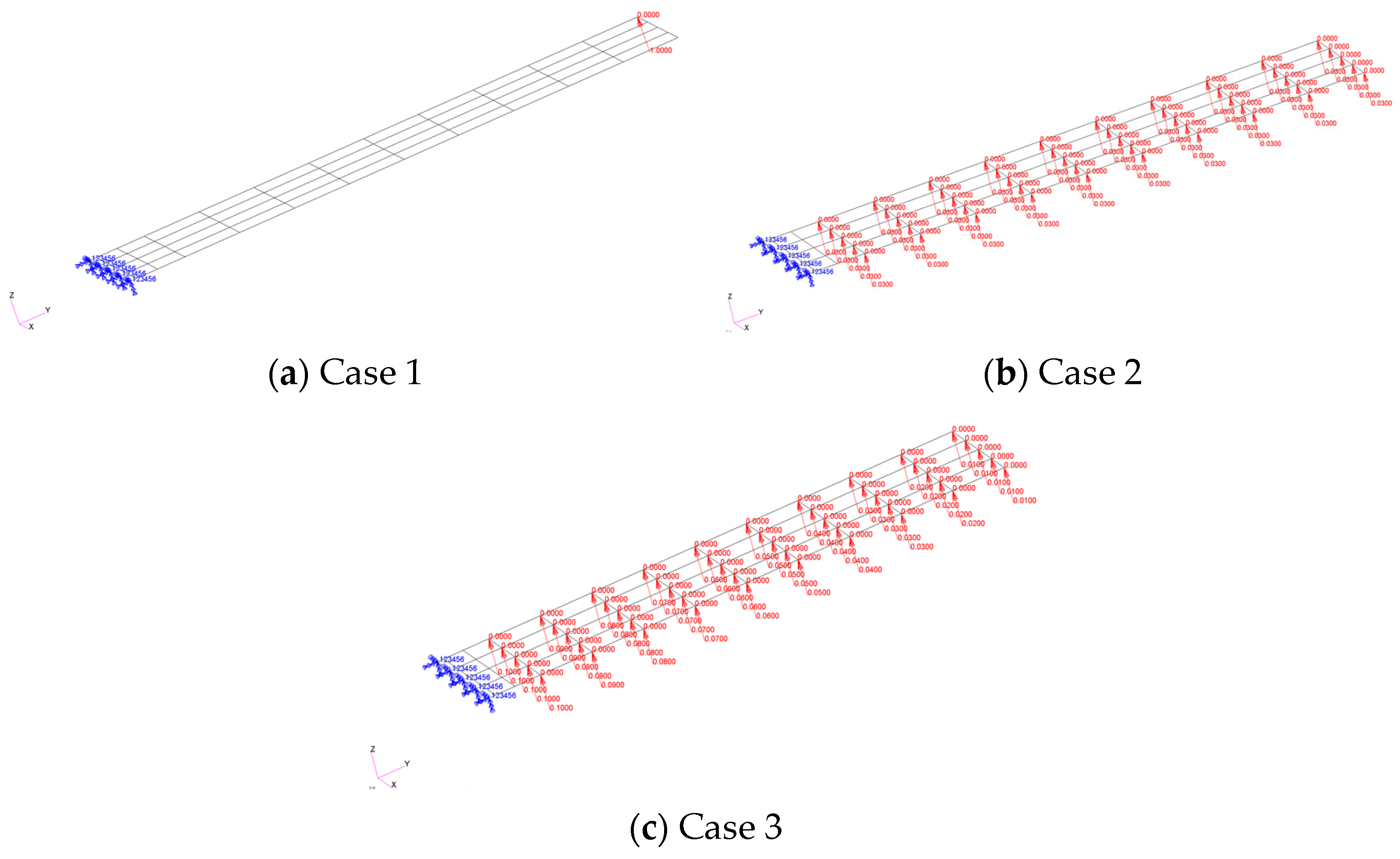
Outside the FSI framework, three load conditions were taken into consideration, listed in Table 2: (1) case 1—a single force acting on one node; (2) case 2—equal forces acting on all nodes; and (3) case 3—proportionally varying forces acting on all nodes, as shown in Figure 5, respectively. For comparability to the load cases inside the FSI framework where the aerodynamic model is shown as in Figure 6, the original structural model is identical, as discussed in Section 2.1.
Table 2.
Load cases outside FSI framework.
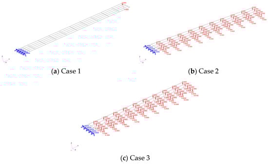
Figure 5.
Load cases outside FSI framework.
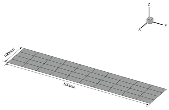
Figure 6.
Aerodynamic model.
- (2)
- Aerodynamic Model Inside the FSI Framework
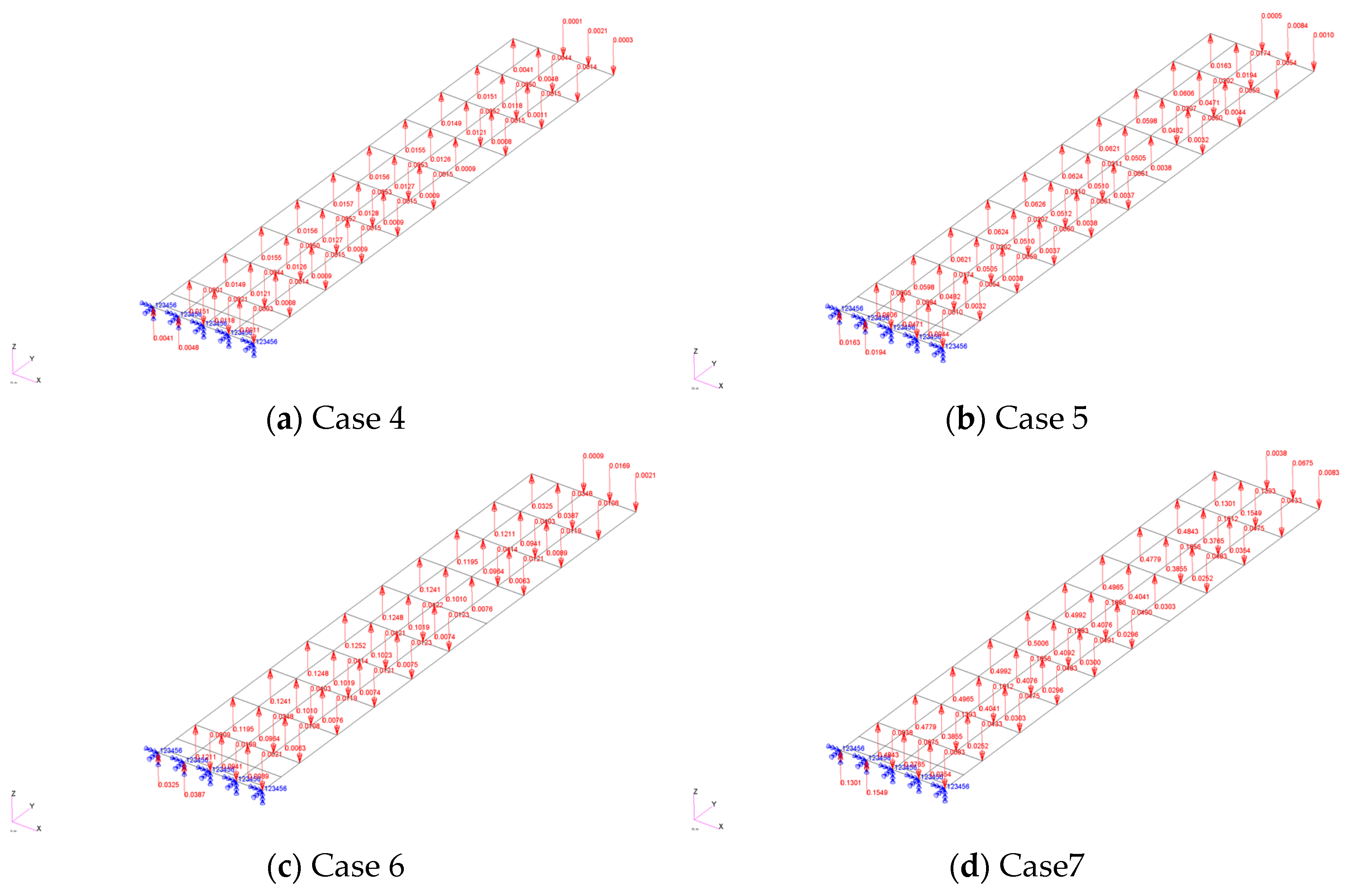
Using the principles outlined in Section 2.4, an aerodynamic model, shown in Figure 6, is established for the structural model discussed in Section 2.1. Four elements are arranged chordwise, and ten elements are arranged spanwise. The aerodynamic loads acting on the structure in the four cases are listed in Table 3 and the corresponding load model is demonstrated in Figure 7.
Table 3.
Aerodynamic conditions.
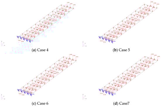
Figure 7.
Aerodynamic loads acting on the first-level substructure in different cases.
3.3. Calculation Process
To validate the proposed method, a simulation process is introduced in this section for the structural and aerodynamic models in Section 2.2. The loads acting on the first-level substructure, denoted as , are displayed in Figure 5 and Figure 7. Modal superposition is used to calculate the displacement of this level, whose mode set with the original constrained boundary is written as . Hence, the static deformation can be written as follows:
Employing Equations (14)–(25), the results of second- and third-level substructures are obtained and compared with the models in Figure 3 and Figure 4, which are solved via MSC.Nastran SOL 101. The displacement comparison is based on the relative error (Re) to evaluate the difference in distribution. In addition, the strain energy of the substructure is determined using Equation (27) to evaluate the entire difference:
where is the -level substructure displacement solved using the proposed method, and is that of MSC.Nastran SOL 101.
To assess the stress using the proposed method, a displacement-based stress solution is generated according to the plane’s stress type in elastic mechanics, as displayed in Equation (28). Specifically, the discrete displacement is utilized in Equation (15) to fit a surface, with a deflection in the z-axis.
where is the x-axis normal stress, is the y-axis normal stress, and is the shear stress. To compare the invariant of stress, the von Mises stress is calculated using Equation (29).
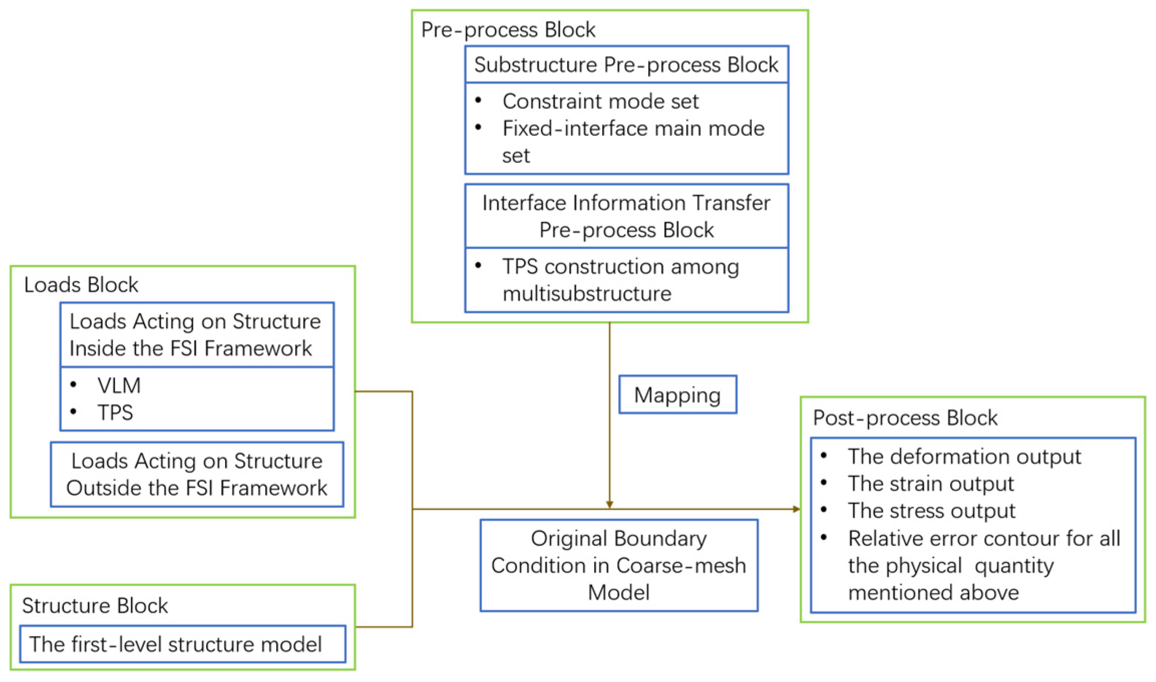
The calculation flowchart is shown in Figure 8.
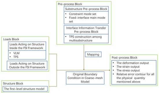
Figure 8.
Calculation flowchart.
4. Results and Discussion
To evaluate the displacement and stress solved using the proposed method, a panel with three-level substructures was built and analyzed using three cases outside the FSI framework, as Figure 5 shows, and four cases inside the FSI framework, as Figure 7 shows. In this section, the results are analyzed from the following aspects: (1) to evaluate necessity, the internal displacement accuracy of the coarse FE model is studied, providing a reference for further results; (2) to investigate adaptivity, the displacement accuracies of several substructures inside the entire model in different positions are compared and discussed; (3) to determine the effectiveness of the displacement assessment, the internal displacement accuracy of the local fine-meshed model is discussed; and (4) to determine the effectiveness of stress assessment, the stress precision of the proposed method is discussed. It is worth noting that we focus on deformation in the z-axis, which is closely related to the stress, as it is significant under aerodynamic loads. The displacement difference between the proposed method and MSC.Nastran is depicted using relative error contours, determined using Equation (26). In addition, the results of cases 1, 2, 3, and 6 are compared and discussed in Section 4.1 and Section 4.2 because the displacement relative error distributions resemble the four load cases inside the FSI framework.
4.1. The Displacement Evaluation of The Coarse Model
- (1)
- The Confidence of Original Displacement Boundary
The relative error of deformation in the z-axis between modal superposition and MSC.Nastran in case 6 is displayed in Figure 9. The contours indicate that the accuracy of the modal superposition is reliable for further investigations with respect to the displacement boundary condition of the coarse-meshed model.
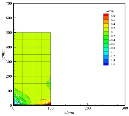
Figure 9.
Relative error of displacement between modal superposition and MSC.Nastran in case 6.
- (2)
- The Displacement Distribution Inside the Coarse Model
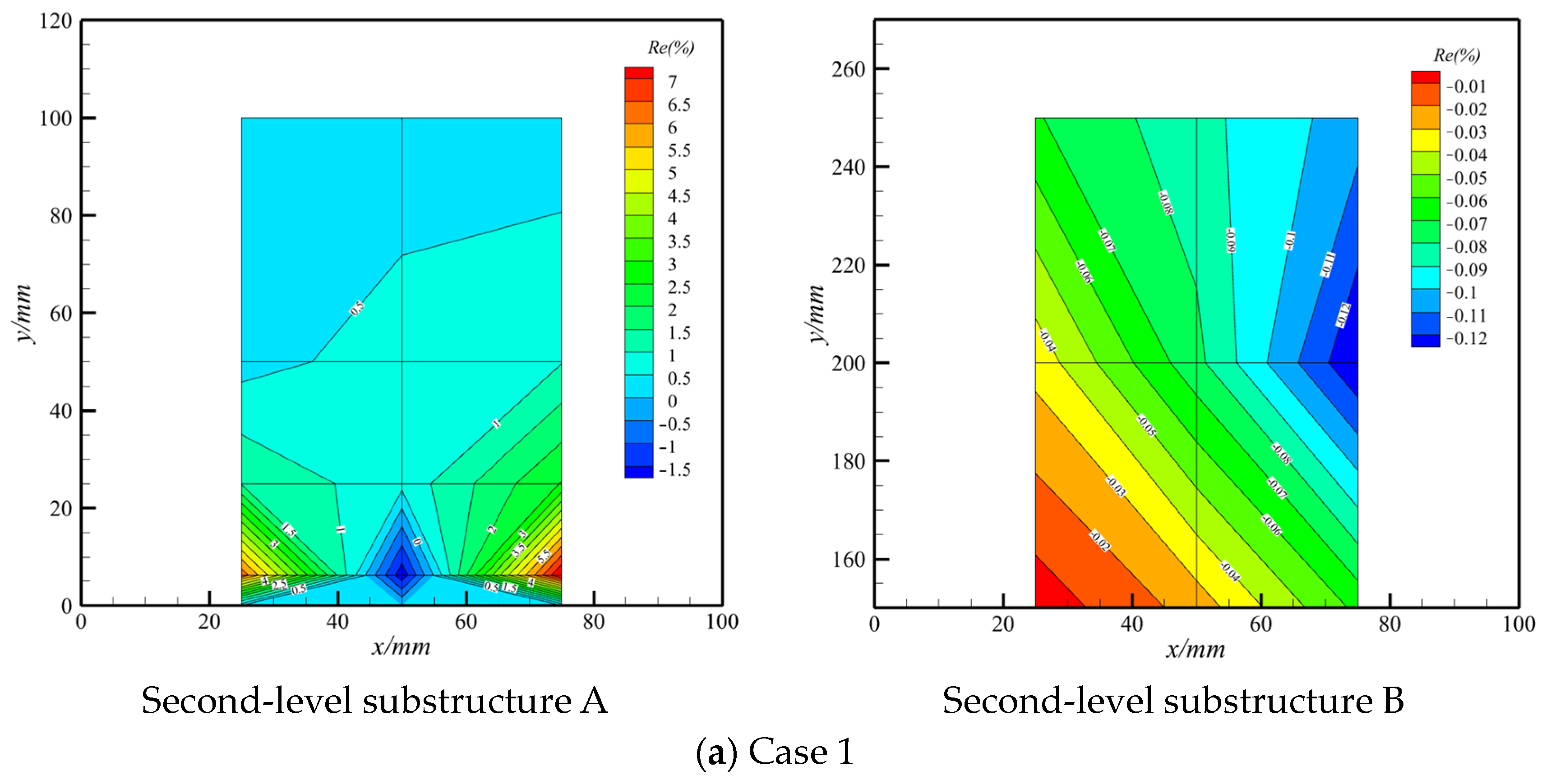
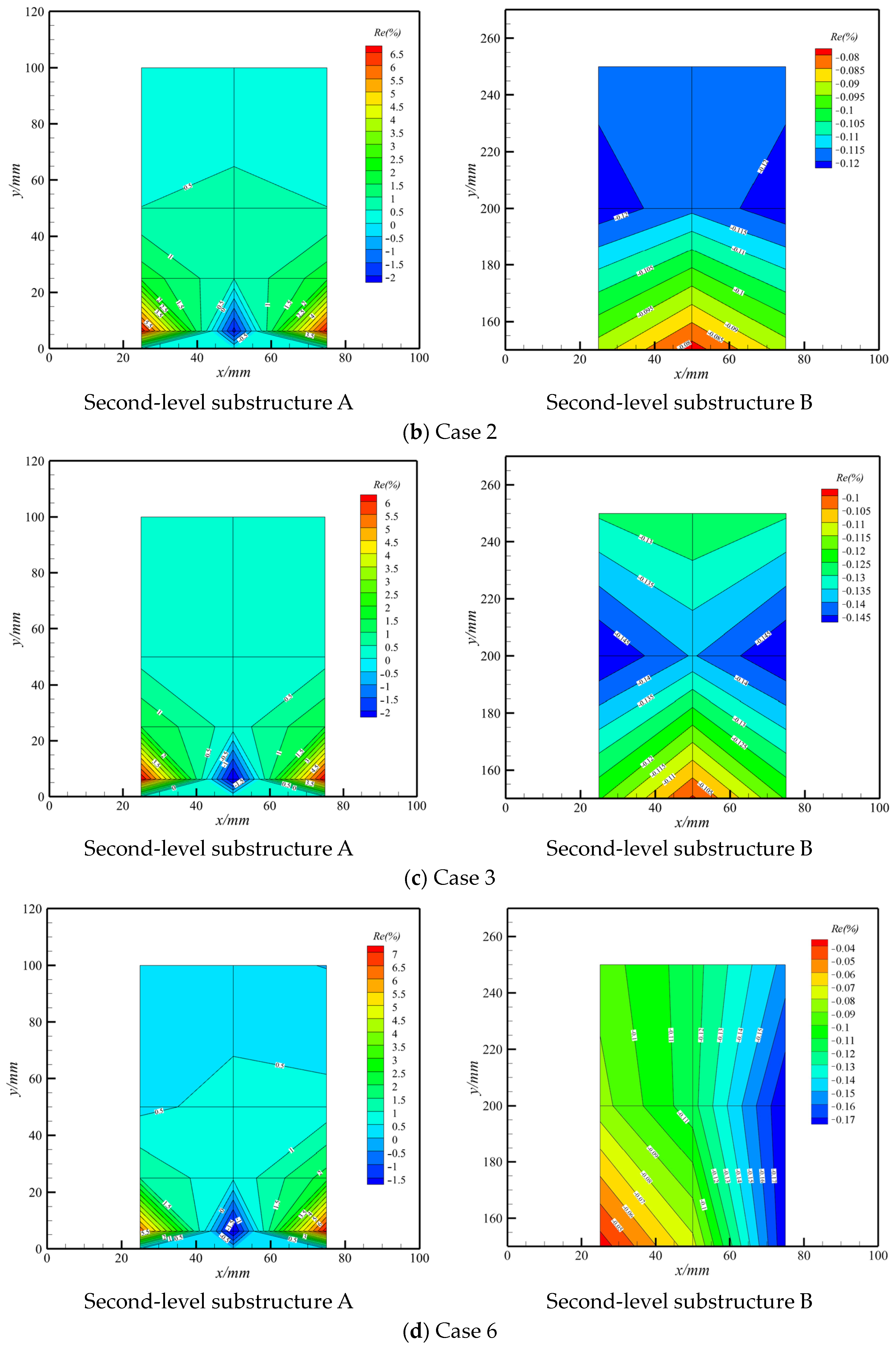
The deformation relative error between substructures A and B and their counterparts in Figure 2 for cases 1, 2, and 3 (outside the FSI framework) and case 6 (inside the FSI framework) is depicted in Figure 10, exhibiting the coarse model’s deformation distribution. As shown in Figure 10, the displacement distribution is quite simple, which allows us to obtain reliable strain and stress values due to the bilinear shape function in coarse elements. Therefore, it is necessary to balance the detailed displacement distribution achievement and efficiency for reliable strain and stress by locally fine mesh.

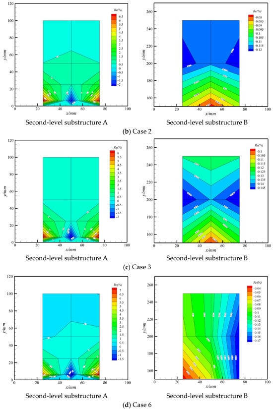
Figure 10.
Relative error of displacement without inner hierarchy.
The locally fine-meshed model is a feasible and reliable method to obtain accurate deformation and strain data by integrating boundary conditions. On the one hand, a fine-meshed model focused on an area can provide comprehensive information regarding mass and stiffness, even working together with a low-order shape function, and the subject orders can be controlled by the selected modals. On the other hand, the boundary conditions provide information for solving the general coordinates of the selected modals to approximate the solution space. Based on the substructure method, a multi-level structure is investigated in Section 4.2 and Section 4.3.
4.2. The Effectiveness of Displacement Assessment
- (1)
- The Adaptivity of Different Positions Inside the Structural Model
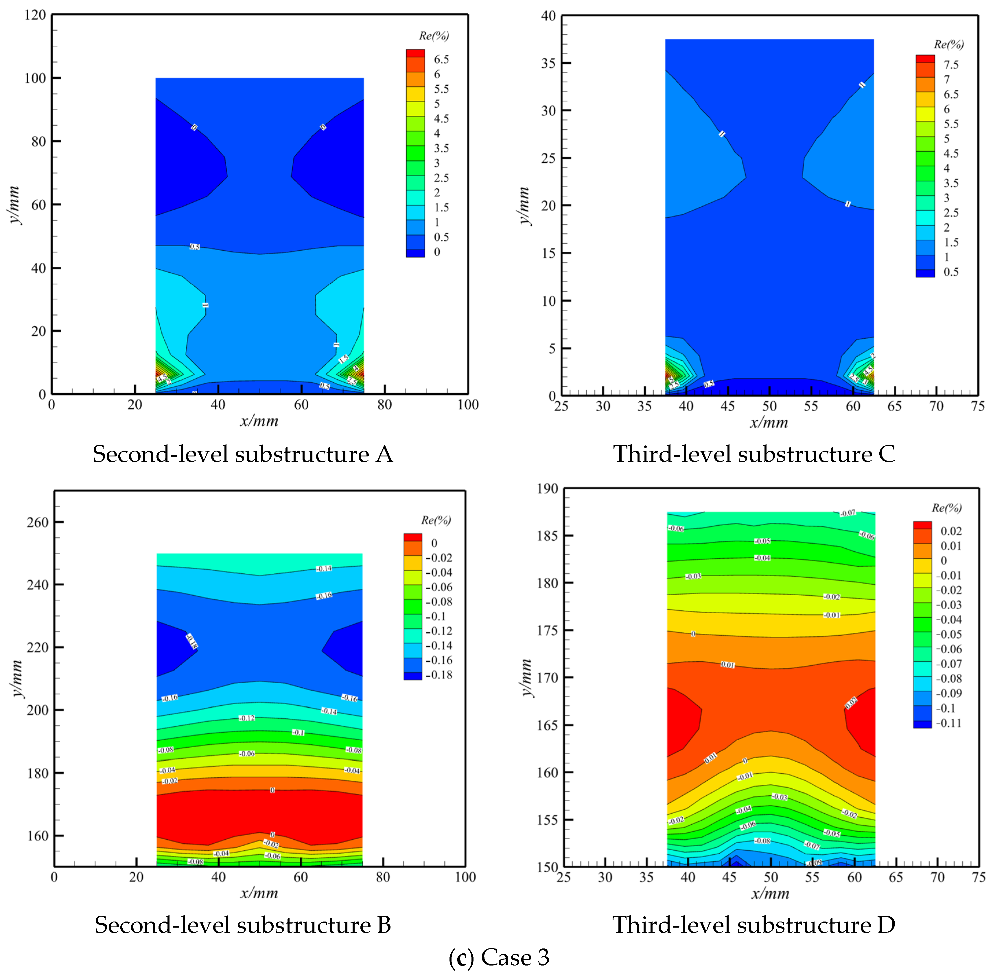
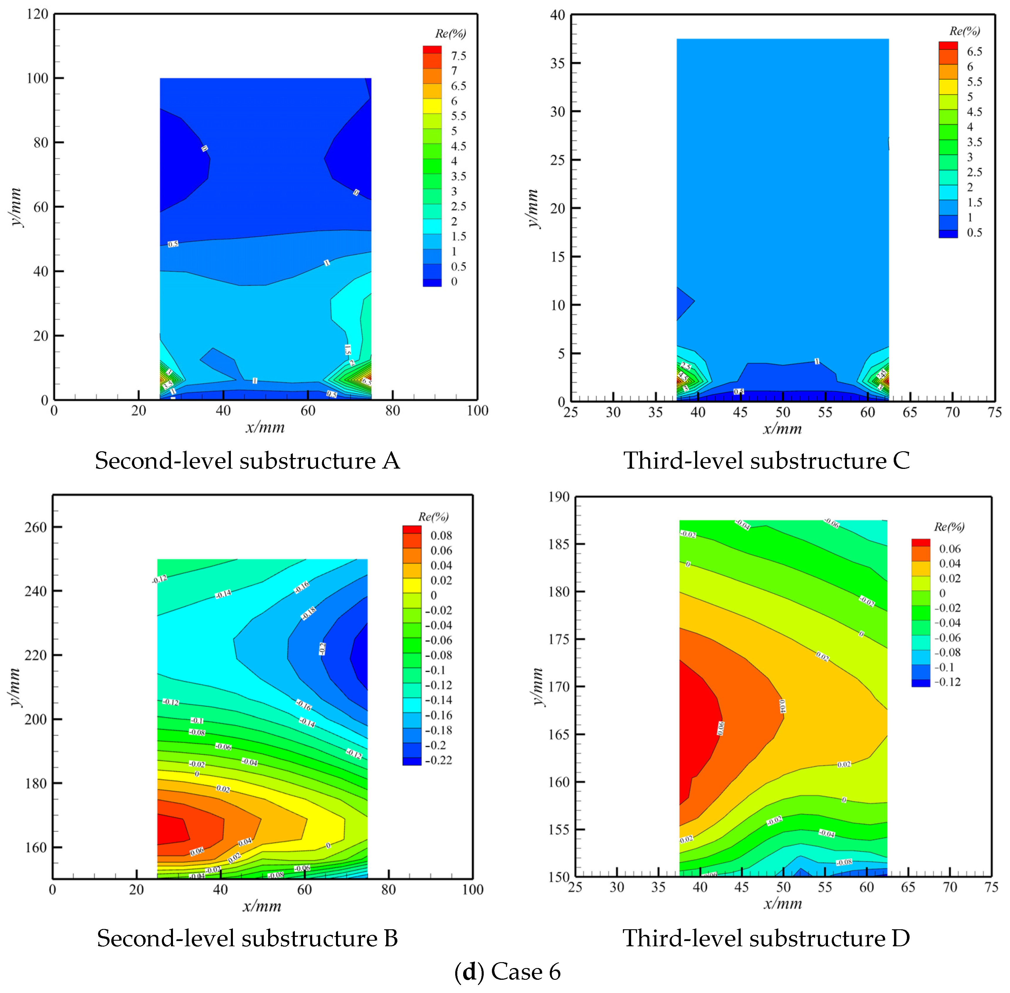
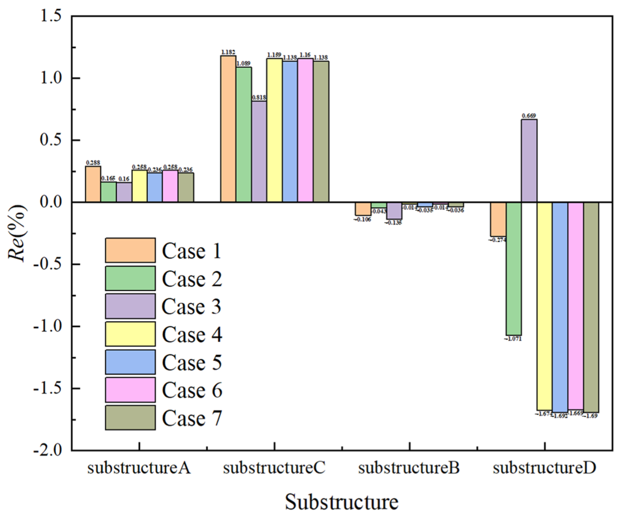
The distributions of displacement difference between the global fine-mesh model (substructures A and B in Figure 3 and substructures C and D in Figure 4) and local fine-mesh and hierarchical models (substructures A, B, C, and D counterparts in Figure 2) are displayed in Figure 11. The results for all displayed cases indicate that the displacement relative error of substructure A is less than 8%, occurring near the constraint boundary, while that of substructure B is between −0.2% and 0.2%. The absolute deformation near the constraint boundary in substructure A is smaller than that of substructure B, which leads to a relatively large relative error, although the absolute error is small. Similar conclusions can be drawn by comparing third-level substructures C and D. Accordingly, the proposed method’s accuracy is acceptable and independent for different substructure positions.
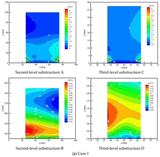
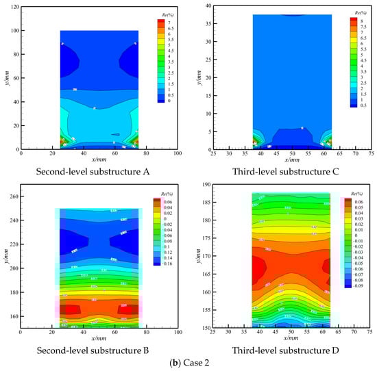
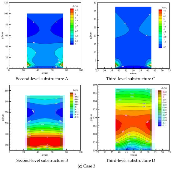

Figure 11.
The relative error of displacement with inner hierarchy.
In addition, as Figure 11 shows, the relative error distribution is consistent with the displacement distribution for all the typical cases. For cases 2 and 3, the displacement distribution and relative error distribution are both longitudinally symmetrical, while the results of cases 1, 4, 5, 6, and 7 exhibit asymmetry. This is because the loads acting on the structure are symmetric for cases 2 and 3, unlike those in cases 1, 4, 5, 6, and 7. Since we considered typical load cases, and the results of the displacement’s relative error distribution are consistent across the different load cases, the adaptivity of the proposed method in displacement assessments is verified with different load cases.
- (2)
- The Inner Displacement Precision for Local Fine-meshed Model
As shown in Figure 11, a comparison between second-level substructure A and third-level substructure C using the same load case indicates that the relative error distribution of substructure C is in accordance with the counterpart in substructure A. The coincidence implies that the local spectrum augmentation for substructure A is beneficial and effective enough for further displacement estimation within it. However, the maximum relative error and distribution form of substructure C resembles that of substructure A, which is attributed to the inherited influence of its former level substructure due to the interpolation sampling.
Cross-comparisons among all the investigated cases reveal that the maximum relative error of the coarse-meshed level model cannot be exaggerated and overamplified when mapping to the fine-meshed level model. Furthermore, the drastic alteration in the relative error is within a smaller range, while most ranges are distributed flat and evenly, which is advantageous for strain assessments. The stable maximum relative error in the structure boundary and the even distribution of relative errors inside the finer-meshed models imply the significant effectiveness of the proposed method.
A comparison between substructures B and D confirms the conclusion mentioned above. It is worth noting that there are barely any significant alterations in the relative error distribution of substructure D and its counterpart in substructure B, which is different from those of substructures C and A. This further demonstrates that the error propagation results from interpolation sampling at the last level, where the displacement relative error is small in substructure B.
Comparing Figure 10 and Figure 11, it can be concluded that the local spectrum augmentation is beneficial for capturing the displacement distribution inside a substructure effectively, which is imperative for the solution’s convergence to the real one. Displacement assessment is a discrete aspect for evaluating the proposed method with respect to detailed distribution, while the strain energy that was determined using Equation (27) provides a global perspective for assessing the mapping’s stability under different load cases.
Figure 12 shows the strain energy of different substructures in all seven cases, both inside and outside the FSI framework. The consistent strain energy of an identical substructure in the seven cases illustrates that the mapping matrix is only related to the model position, which is advantageous for mapping storage and transformations in different cases. Given that the acceptable precision and mapping stability are realized in different positions and cases for the proposed method, the prominent advantage stands for modular analysis.
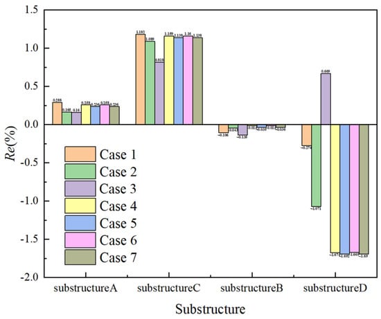
Figure 12.
Relative error of strain energy in different working conditions.
The coarse-meshed model is developed and analyzed once to extract the boundary conditions for the following fine-meshed models despite its simultaneity and region of interest, which lays a solid foundation for addressing the time-dependent problem. Substructures A, B, C, and D were studied to validate the proposed method regarding deformation analysis; the next section focuses on stress assessments.
4.3. The Effectiveness in Strain Assessment
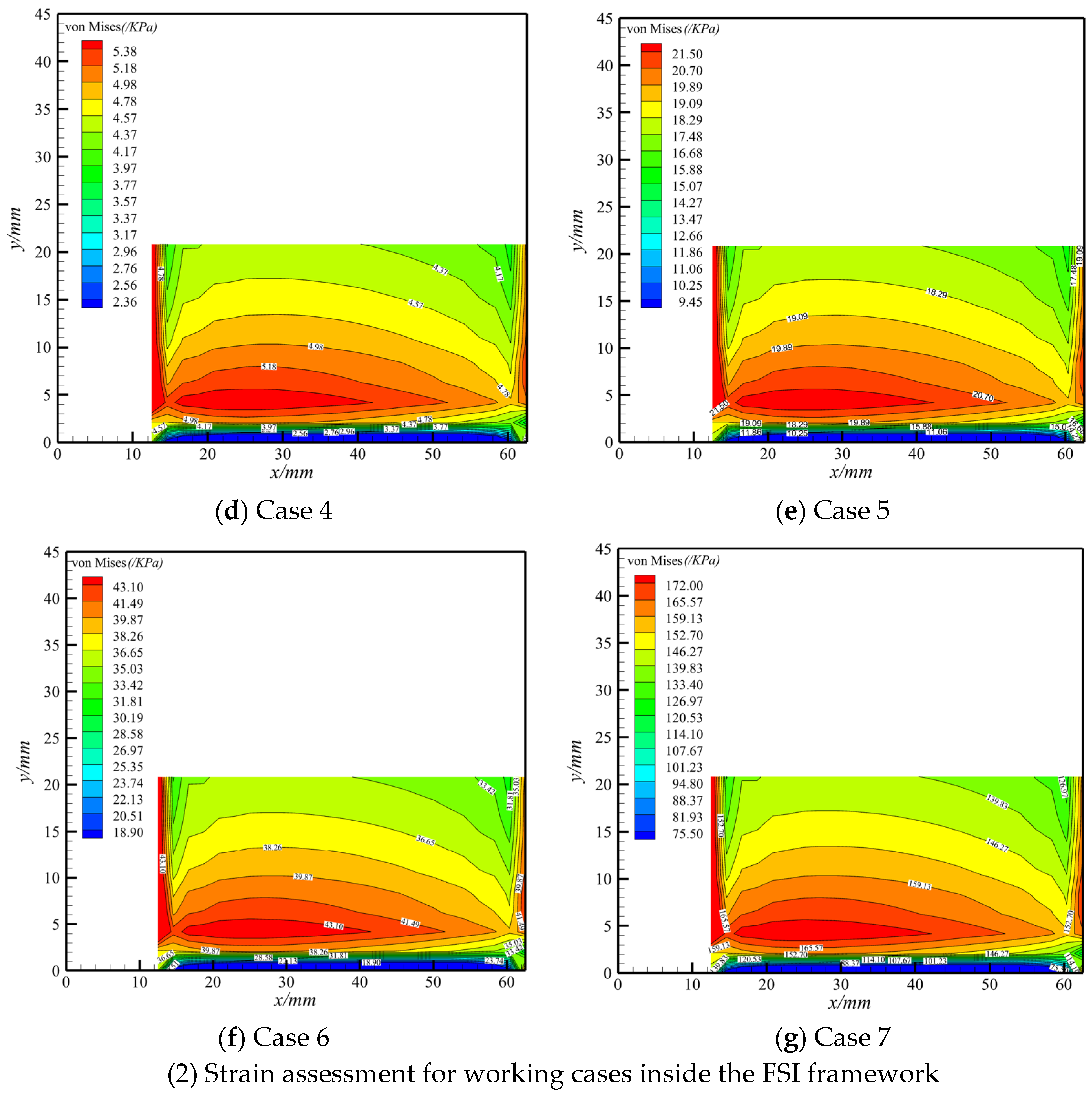
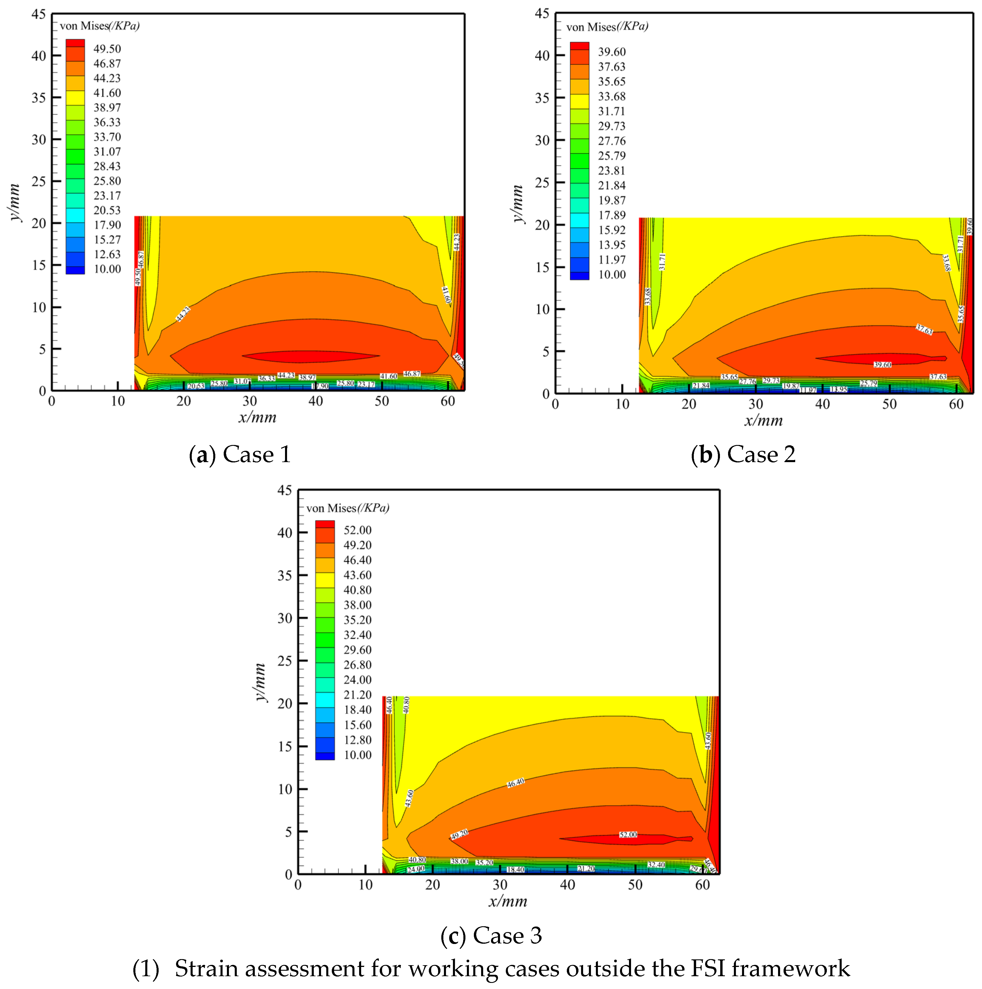
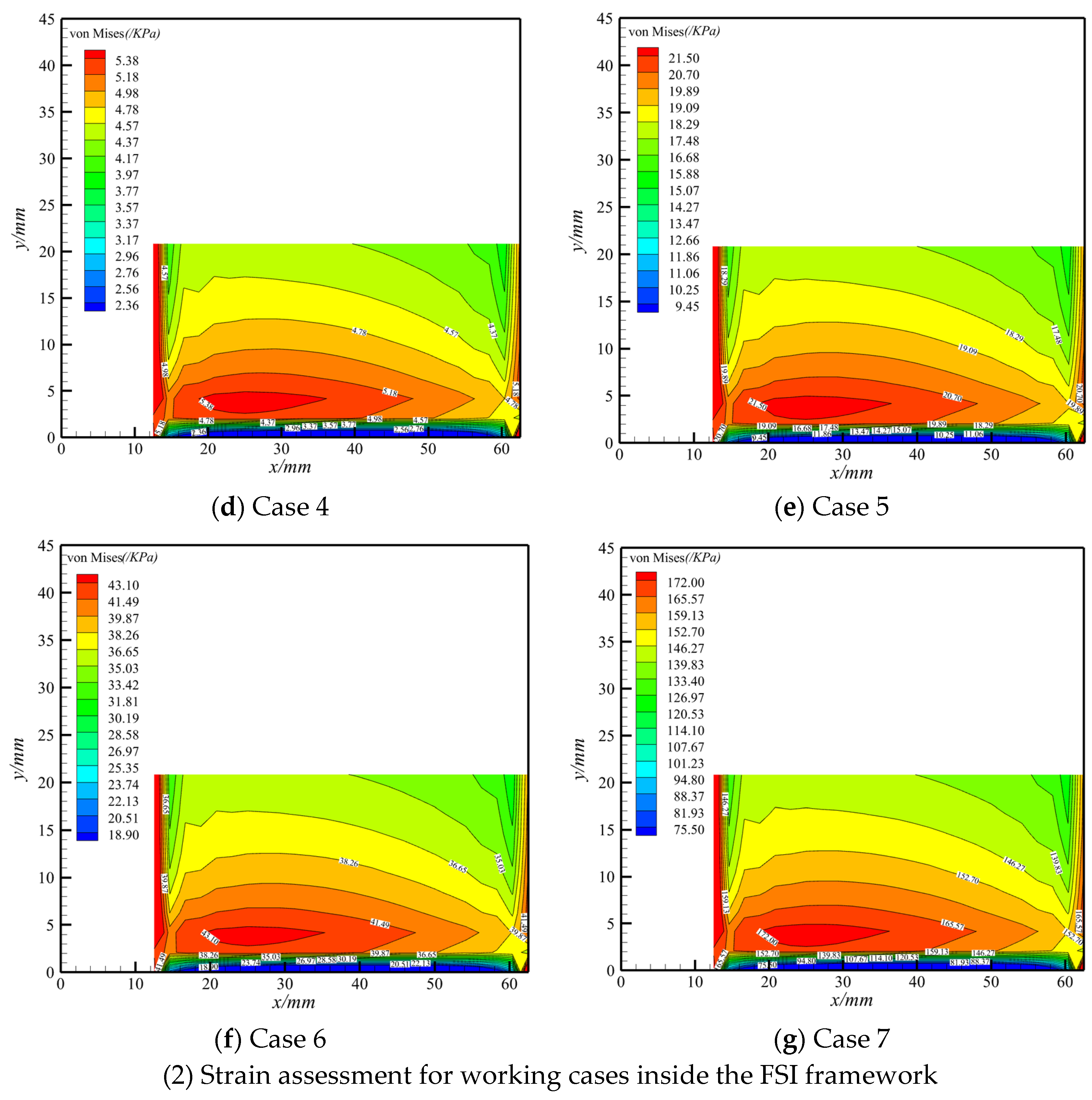
The displacement assessment is discussed and analyzed in Section 4.2, and it is imperative for strain assessments. In this section, the strain assessments are conducted for cases outside and inside the FSI framework. For strength assessments, the stress of the critical position is investigated. Specifically, the stress assessment of substructure F (Figure 4) is analyzed because the aerodynamic center is located a quarter chordwise, and the nearby constraint boundary suffers from heavy stress compared with other regions. The von Mises stresses determined using the proposed method in all seven cases are displayed in Figure 13 and compared with the results of MSC.Nastran SOL 101 in Figure 14. These values were obtained using Equations (28) and (29), respectively.
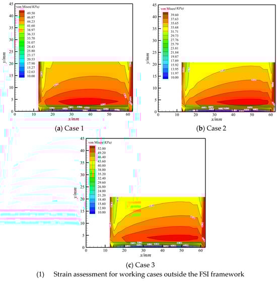
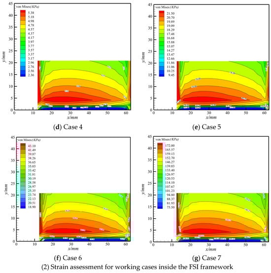
Figure 13.
Stress assessment using the proposed method.

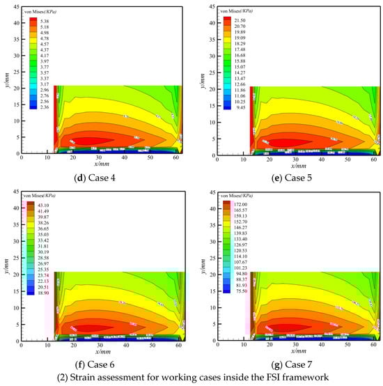
Figure 14.
Stress assessment by MSC.Nastran SOL 101.
The stress assessment outside the FSI framework from case 1 to case 3 is displayed in Figure 13(1) and Figure 14(1), and a satisfactory approximation for all typical load conditions was obtained. Regarding the stress assessment within the FSI framework, as shown in Figure 13(2) and Figure 14(2), the maximum stress appears near a one-quarter chordwise area, which is not only consistent with the engineering application, but the little distinction also highlights the effectiveness of the proposed method for stress achievement inside the FSI framework. Although the maximum von Mises region predicted using the proposed method is slightly larger than that of the MSC.Nastran, more conservative results regarding critical position estimation were obtained. To summarize, the stress assessment using the proposed method is reliable, as proved by the analysis of typical working conditions inside and outside the FSI framework.
5. Conclusions
In this paper, a multisubstructure-based method was proposed, and the displacement and stress assessment were analyzed for situations both outside and inside the FSI framework by integrating steady VLM. A three-level substructure panel is established to verify the proposed method, and the following conclusions were drawn:
- (1)
- The proposed method can effectively depict the displacement inside the structure. The displacement boundary of the fine-meshed model can be determined via a combination of TPS and eigenvector augmentation inside the last-level substructure. Moreover, the displacement inside the model is assessed by integrating the fixed-interface main mode and the corresponding generalized coordinates based on the principle of minimum potential energy.
- (2)
- The maximum displacement relative error occurs near the constraint boundary, with small displacement and therefore a large relative error, in contrast to the absolute error. The reason is that the displacement error is inherited from the last-level substructure via interpolation sampling. However, this error can be reduced by narrowing the substructure inside, from the top level to the bottom. A more accurate substructure displacement boundary can be determined when it is located inside its last-level substructure because the displacement accuracy of the last-level substructure is improved by adding higher-order shape functions.
- (3)
- The analysis results of different loads and substructure positions highlight the reliability of the method, which only considers the mapping range and location such that the mapping information can be stored and transferred when required. Given the accuracy and efficiency of the proposed method, this study lays a solid foundation for addressing the time-dependent problem in the analysis of fluid–structure interactions.
Author Contributions
Conceptualization, C.X., K.H. and Z.Z.; methodology, K.H.; software, K.H. and N.G.; validation, K.H. and Y.M.; formal analysis, K.H. and C.X.; investigation, C.X.; resources, C.X.; data curation, Y.M.; writing—original draft preparation, K.H.; writing—review and editing, C.X., Z.Z., Y.M. and N.G.; visualization, K.H. and Y.M.; supervision, C.X.; project administration, Z.Z.; funding acquisition, Y.M. All authors have read and agreed to the published version of the manuscript.
Funding
Frontier Cross-Fund Project of Beihang University.
Data Availability Statement
No new data were created or analyzed in this study. Data sharing is not applicable to this article.
Conflicts of Interest
The authors declare no conflicts of interest.
References
- Karpel, M.; Brainin, L. Stress considerations in reduced-size aeroelastic optimization. AIAA J. 1995, 33, 716–722. [Google Scholar] [CrossRef]
- Piperni, P.; DeBlois, A.; Henderson, R. Development of a multilevel multidisciplinary-optimization capability for an industrial environment. AIAA J. 2013, 51, 2335–2352. [Google Scholar] [CrossRef]
- Taylor, R. The role of optimization in component structural design: Application to the F-35 joint strike fighter. In Proceedings of the 25th International Congress of the Aeronautical Sciences, Hamburg, Germany, 3–8 September 2006. [Google Scholar]
- Corrado, G.; Ntourmas, G.; Sferza, M.; Traiforos, N.; Arteiro, A.; Brown, L.; Chronopoulos, D.; Daoud, F.; Glock, F.; Ninic, J.; et al. Recent progress, challenges and outlook for multidisciplinary structural optimization of aircraft and aerial vehicles. Prog. Aerosp. Sci. 2022, 135, 100861. [Google Scholar] [CrossRef]
- Livne, E.; Schmit, L.A.; Friedmann, P.P. Integrated structure/control/aerodynamic synthesis of actively controlled composite wings. J. Aircr. 1993, 30, 387–394. [Google Scholar] [CrossRef]
- Bindolino, G.; Lanz, M.; Mantegazza, P.; Ricci, S. Integrated structural optimization in the preliminary aircraft design. In Proceedings of the 17th Congress of the International Council of the Aeronautical Sciences, Stockholm, Sweden, 9–14 September 1990; pp. 1366–1378. [Google Scholar]
- Noor, A.K.; Lowder, H.E. Approximate techniques of structural reanalysis. Comput. Struct. 1974, 4, 801–812. [Google Scholar] [CrossRef]
- Cameron, C.J.; Lind, E.; Wennhage, P.; Göransson, P. Proposal of a methodology for multidisciplinary design of multifunctional vehicle structures including an acoustic sensitivity study. Int. J. Veh. Struct. Syst. 2009, 1, 3. [Google Scholar] [CrossRef]
- Jonsson, E.; Riso, C.; Lupp, C.A.; Cesnik, C.E.S.; Martins, J.R.R.A.; Epureanu, B.I. Flutter and post-flutter constraints in aircraft design optimization. Prog. Aerosp. Sci. 2019, 109, 100537. [Google Scholar] [CrossRef]
- Li, Q.Y.; Li, G.; Wei, Y.T.; Ran, Y.; Wu, B.; Tan, G.; Li, Y.; Chen, S. Review of aeroelasticity design for advanced fighter. Acta Aeronaut. Astronaut. Sin. 2020, 41, 523430. [Google Scholar]
- Verri, A.A.; Luiz Bussamra, F.; Cesnik, C.E. Outcomes of Nonlinear Static Aeroelasticity for Wing Stress and Buckling Applied to a Transport Aircraft. In Proceedings of the AIAA SciTech 2024 Forum, Orlando, FL, USA, 8–12 January 2024; p. 2447. [Google Scholar]
- Capuano, G.; Ruzzene, M.; Rimoli, J.J. Modal-based finite elements for efficient wave propagation analysis. Finite Elem. Anal. Des. 2018, 145, 10–19. [Google Scholar] [CrossRef]
- Craig, R.R.; Bampton, M.C.C. Coupling of substructures for dynamic analyses. AIAA J. 1968, 6, 1313–1319. [Google Scholar] [CrossRef]
- Hurty, W.C. Vibrations of structural systems by component mode synthesis. J. Eng. Mech. Div. 1960, 86, 51–69. [Google Scholar] [CrossRef]
- Hurty, W.C. Dynamic analysis of structural systems using component modes. AIAA J. 1965, 3, 678–685. [Google Scholar] [CrossRef]
- Hintz, R.M. Analytical methods in component modal synthesis. AIAA J. 1975, 13, 1007–1016. [Google Scholar] [CrossRef]
- Rubin, S. Improved component-mode representation for structural dynamic analysis. AIAA J. 1975, 13, 995–1006. [Google Scholar] [CrossRef]
- Craig, R.R.; Chang, C.-J. Free-Interface Methods of Substructure Coupling for Dynamic Analysis. AIAA J. 1976, 14, 1633–1635. [Google Scholar] [CrossRef]
- Craig, R.R.; Chang, C.-J. A review of substructure coupling methods for dynamic analysis. In Proceedings of the 13th Annual Meeting of the Society of Engineering Science, Hampton, VA, USA, 1–3 November 1976; NASA’s Langley Research Center: Hampton, VA, USA, 1976; pp. 393–408. [Google Scholar]
- Craigr, R.; Chang, C.-J. On the use of attachment modes in substructure coupling for dynamic analysis. In Proceedings of the 18th Structural Dynamics and Materials Conference, San Diego, CA, USA, 21–23 March 1977; AIAA: San Diego, CA, USA, 1977; pp. 89–99. [Google Scholar]
- Babuška, I.; Griebel, M.; Pitkäranta, J. The problem of selecting the shape functions for ap-type finite element. Int. J. Numer. Methods Eng. 1989, 28, 1891–1908. [Google Scholar] [CrossRef]
- Zander, N.; Bog, T.; Kollmannsberger, S.; Schillinger, D.; Rank, E. Multi-level hp-adaptivity: High-order mesh adaptivity without the difficulties of constraining hanging nodes. Comput. Mech. 2015, 55, 499–517. [Google Scholar] [CrossRef]
- Zhu, D.C. Development of hierarchical finite element methods at BIAA. In The International Conference on Computational Mechanics; Springer: Tokyo, Japan, 1986. [Google Scholar]
- Bardell, N.S. The application of symbolic computing to the hierarchical finite element method. Int. J. Numer. Methods Eng. 1989, 28, 1181–1204. [Google Scholar] [CrossRef]
- Harder, R.L.; Desmarais, R.N. Interpolation using surface splines. J. Aircr. 1972, 9, 189–191. [Google Scholar] [CrossRef]
- Yang, C.; Wang, L.B.; Xie, C.C.; Liu, Y. Aeroelastic trim and flight loads analysis of flexible aircraft with large deformations. Sci. China Technol. Sci. 2012, 55, 2700–2711. [Google Scholar] [CrossRef]
- Xie, C.C.; Yang, L.; Liu, Y.; Chao, Y. Stability of very flexible aircraft with coupled nonlinear aeroelasticity and flight dynamics. J. Aircr. 2018, 55, 862–874. [Google Scholar]


Disclaimer/Publisher’s Note: The statements, opinions and data contained in all publications are solely those of the individual author(s) and contributor(s) and not of MDPI and/or the editor(s). MDPI and/or the editor(s) disclaim responsibility for any injury to people or property resulting from any ideas, methods, instructions or products referred to in the content. |
© 2024 by the authors. Licensee MDPI, Basel, Switzerland. This article is an open access article distributed under the terms and conditions of the Creative Commons Attribution (CC BY) license (https://creativecommons.org/licenses/by/4.0/).