Tau Theory-Based Flare Control in Autonomous Helicopter Autorotation

Abstract

A novel trajectory generation and control architecture for fully autonomous autorotative flare that combines rapid path generation with model-based control is proposed. The trajectory generation component uses optical Tau theory to compute flare trajectories for both longitudinal and vertical speed. These flare trajectories are tracked using a nonlinear dynamic inversion (NDI) control law. One convenient feature of NDI is that it inverts the plant model in its feedback linearization loop, which eliminates the need for gain scheduling. However, the plant model used for feedback linearization still needs to be scheduled with the flight condition. This key aspect is leveraged to derive a control law that is scheduled with linearized models of the rotorcraft flight dynamics obtained in steady-state autorotation, while relying on a single set of gains. Computer simulations are used to demonstrate that the NDI control law is able to successfully execute autorotative flare in the UH-60 aircraft. Autonomous flare trajectories are compared to piloted simulation data to assess similarities and discrepancies between piloted and automatic control approaches. Trade studies examine which combinations of downrange distances and altitudes at flare initiation result in successful autorotative landings.

1. Introduction

Autorotation is a complex maneuver that helicopter pilots must perform in the event of engine or transmission failure. Recently, there has been increasing interest in automating helicopter autorotation maneuvers. The automation of helicopter autorotation has several potential applications: the execution of maneuvers on rotory-wing unmanned aerial vehicles [1], the creation of pilot cueing displays [2,3,4,5,6,7,8,9,10], and the prediction of the height–velocity diagram [11] via simulation. The two main phases of autorotation consist of a steady-state descent phase, in which the aircraft uses the inflow induced by vertical descent to maintain rotor speed within an acceptable range, and the flare, in which rotor kinetic energy is traded for a reduction in the aircraft’s forward and vertical speeds. These phases are shown qualitatively in Figure 1. The steady-state descent phase of the maneuver is fairly straightforward to automate in the sense that the aircraft state can be driven to the known autorotative trim state using standard feedback control techniques [12]. The challenge of automating the steady-state descent phase largely lies in planning a path to the selected landing point; this problem has been addressed in [6,7,13]. Conversely, the flare maneuver is particularly difficult to automate due to the competing state constraints between forward, vertical, and rotor speeds. In addition, the flare maneuver must be timed, scaled, and tailored according to the vehicle state condition as it nears the ground. For instance, if the aircraft initiates autorotation from a low speed and low altitude, the resulting flare maneuver will be short and will focus on rapidly arresting the vertical descent just before the vehicle touches down. In contrast, autorotations starting from high-energy flight conditions (higher altitude and/or higher speeds) require a more gradual flare initiated from a higher altitude.

Several authors have attempted to derive control laws for autorotation flare that adapt to the vehicle energy state as it nears the ground. This includes work by Langelaan et al. [14], Sunberg et al. [1], and Eberle and Rogers [15]. Despite the existing work in this area, there remains a need to develop flare control laws that can be computed online in real time and that use some type of model-based control to ensure that competing constraints on rotor and vehicle speeds are satisfied as much as possible. This work introduces a new trajectory generation and control architecture that combines rapid path generation with model-based control. The trajectory generation component of the architecture is similar to that proposed by Eberle and Rogers [15]. This trajectory generation scheme uses optical Tau theory [16] to rapidly compute a solution to a two-point boundary value problem encompassing the initial vehicle state at flare initiation and the desired final vehicle state at touchdown. While in [15] this trajectory generator was envisioned primarily for pilot cueing, in the current work, an automatic control loop is designed, which tracks the desired trajectory to perform an autonomous flare.

The flight control law used in this work to track the desired flare trajectory is nonlinear dynamic inversion (NDI), a popular model-following scheme among aircraft and rotorcraft manufacturers, and within the aerospace flight control community in general. Application of NDI control laws to rotorcraft can be found in, e.g., [17,18,19,20,21,22,23,24,25,26]. One convenient feature of NDI is that it inverts the plant model in its feedback linearization loop, which, compared to other more conventional model-following control strategies such as explicit model following (EMF), eliminates the need for gain scheduling. However, the plant model used for feedback linearization still needs to be scheduled with the flight condition. NDI has also been applied to rotorcraft autorotation problems in a limited number of studies [6,12], but its use as a control law in autorotative flare has not been studied extensively to date.

As such, the objective of this study is to develop a trajectory planning and control algorithm for the autorotation flare that is capable of real-time implementation, adaptable to different entry conditions, and uses model-based control to satisfy competing state constraints. The two major contributions included in this paper are the following: (i) the extension of optical Tau theory to generate both longitudinal and vertical speed flare trajectories and (ii) the derivation of an NDI control law specifically intended for flare maneuvers that are scheduled with the linearized rotorocraft flight dynamics obtained in steady-state autorotation at varying speeds.

The paper begins with a description of the six-degrees-of-freedom helicopter simulation model representative of a utility helicopter similar to a UH-60 used in control law development and simulation analysis. This is followed by detailed descriptions of the trajectory generation algorithm and DI control law. Simulation results demonstrate that the controller is able to successfully execute autorotative flare in the UH-60 aircraft. Autonomous flare trajectories are qualitatively compared to piloted simulation data to assess similarities and discrepancies between piloted and automatic control approaches. Trade studies examine the ability to extend or shorten the flare to reach a desired landing point.

2. Simulation Model

The helicopter flight dynamics model is a MATLAB^® implementation of the helicopter model described in [27] and is representative of a utility helicopter similar to a UH-60. Table 1 summarizes the salient characteristics of the UH-60-like simulation model. The model contains a six-degrees-of-freedom nonlinear rigid-body dynamic model of the fuselage, a quasi-static model of the blade flapping motion, and uses static aerodynamic models for fuselage, tail rotor inflow, and empennage. The main rotor inflow is modeled with a one-state dynamic inflow model [28]. An additional degree of freedom is provided by the main rotor angular speed. The state vector is given by:

$${\mathit{x}}^T=\left[uvwpqr\varphi \theta \psi xyz{\lambda }_0\Omega \right]$$

(1)

where:

u, v, and w are the body-fixed velocities;

p, q, and r are the angular rates;

$\varphi$, $\theta$, and $\psi$ are the Euler angles;

x, y, and z describe the position of the helicopter in the inertial frame;

${\lambda }_0$ is the main rotor inflow;

$\Omega$ is the main rotor angular speed.

The control vector is:

$${\mathit{u}}^T=\left[{\theta }_{1c}{\theta }_{1s}{\theta }_0{\theta }_{0T}\right]$$

(2)

where ${\theta }_{1c}$ and ${\theta }_{1s}$ are the lateral and longitudinal cyclic inputs, ${\theta }_0$ is the collective input, and ${\theta }_{0T}$ is the tail rotor collective. It is worth noting that, because the helicopter model is only used in (unpowered) autorotation conditions in this study, no engine model and throttle inputs are included. A simple ground effect model is used to modify the thrust coefficient of the helicopter in proximity to the ground [29].

Table 1. General characteristics of the UH-60-like utility helicopter model [30].

Parameter	Value	Units
Mass and inertia
Gross weight, W	16,270	lb
Roll-axis moment of inertia, $I_{xx}$	5000	sl-ft2
Pitch-axis moment of inertia, $I_{yy}$	39,000	sl-ft2
Yaw-axis moment of inertia, $I_{zz}$	39,000	sl-ft2
Roll/yaw-axes product of inertia, $I_{xz}$	1900	sl-ft2
Main rotor
Number of blades, $N_{\mathrm{b}}$	4	-
Radius, R	$26.8$	ft
Blade chord, c	$1.73$	ft
Blade twist, ${\theta }_{\mathrm{tw}}$	−13	deg
Flapping hinge offset	1.25	ft
Blade weight, $W_{\mathrm{b}}$	256.9	lb
Blade first mass moment, $M_{\beta }$	86.7	sl-ft
Blade second mass moment, $I_{\beta }$	1512.6	sl-ft2
Angular speed, $\Omega$	27	rad/s
Tail rotor
Number of blades, $N_{{\mathrm{b}}_{\mathrm{TR}}}$	4	-
Radius, $R_{\mathrm{TR}}$	$5.5$	ft
Blade chord, $c_{\mathrm{TR}}$	$0.81$	ft
Blade twist, ${\theta }_{{\mathrm{tw}}_{\mathrm{TR}}}$	−17	deg
Blade second mass moment, $I_{{\beta }_{\mathrm{TR}}}$	$3.10$	sl-ft
Angular speed, ${\Omega }_{\mathrm{TR}}$	$124.62$	rad/s

Table 1. General characteristics of the UH-60-like utility helicopter model [30].

Parameter	Value	Units
Mass and inertia
Gross weight, W	16,270	lb
Roll-axis moment of inertia, $I_{xx}$	5000	sl-ft2
Pitch-axis moment of inertia, $I_{yy}$	39,000	sl-ft2
Yaw-axis moment of inertia, $I_{zz}$	39,000	sl-ft2
Roll/yaw-axes product of inertia, $I_{xz}$	1900	sl-ft2
Main rotor
Number of blades, $N_{\mathrm{b}}$	4	-
Radius, R	$26.8$	ft
Blade chord, c	$1.73$	ft
Blade twist, ${\theta }_{\mathrm{tw}}$	−13	deg
Flapping hinge offset	1.25	ft
Blade weight, $W_{\mathrm{b}}$	256.9	lb
Blade first mass moment, $M_{\beta }$	86.7	sl-ft
Blade second mass moment, $I_{\beta }$	1512.6	sl-ft2
Angular speed, $\Omega$	27	rad/s
Tail rotor
Number of blades, $N_{{\mathrm{b}}_{\mathrm{TR}}}$	4	-
Radius, $R_{\mathrm{TR}}$	$5.5$	ft
Blade chord, $c_{\mathrm{TR}}$	$0.81$	ft
Blade twist, ${\theta }_{{\mathrm{tw}}_{\mathrm{TR}}}$	−17	deg
Blade second mass moment, $I_{{\beta }_{\mathrm{TR}}}$	$3.10$	sl-ft
Angular speed, ${\Omega }_{\mathrm{TR}}$	$124.62$	rad/s

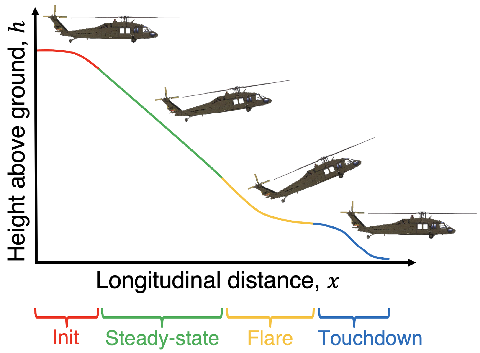
3. Trajectory Generation

A key problem in the flare phase of autorotation is to generate trajectories that can be feasibly tracked by the helicopter while ensuring that the helicopter has minimal longitudinal and vertical speeds at a desired downrange distance and at an altitude of a few feet over the ground (i.e., at the target landing point). In the presented context, downrange distance is the longitudinal distance from the final touchdown longitudinal position. The approach that this paper utilizes is the optical Tau theory [16]. Tau theory was chosen as it offers simple and deterministic mathematics that is computationally inexpensive. It has been previously shown to be capable of modeling other flight maneuvers like helicopter pilots stopping, turning, and pulling up [27,31], and for fixed wing pilots in the landing flare [32]. In the context of helicopter flare maneuvers, it can be shown that longitudinal speed trajectories can be generated using the following equation [15,33]:

$$V_x\left(t\right)=\left[V_x\left(0\right)-V_x\left(\widehat{T}\right)\right]{\left[1-{\displaystyle \frac{(k_{{\mathrm{opt}}_1}-1)\left[V_x\left(0\right)-V_x\left(\widehat{T}\right)\right]t}{x\left(0\right)}}\right]}^{-1-\frac{1}{k_{{\mathrm{opt}}_1}-1}}+V_x\left(\widehat{T}\right)$$

(3)

where t is the time since the initiation of the flare, $\widehat{T}$ is the total time of the maneuver, x is downrange distance, $k_{{\mathrm{opt}}_1}$ is a parameter that dictates the shape of the trajectory, and $V_x\left(\widehat{T}\right)$ is the final (small) longitudinal speed of the vehicle at touchdown. Given an initial downrange distance and longitudinal speed, and a total time to complete the deceleration, $k_{{\mathrm{opt}}_1}$ can be solved for in a deterministic manner by following the method in [15]. It is worth noting that $k_{{\mathrm{opt}}_1}\in \left[-1,1\right]$. Previous approaches, such as the one in [15], used simple exponential trajectories for the vertical speed of the form:

$$V_z\left(t\right)=\left[V_z\left(0\right)-V_z\left(\widehat{T}\right)\right]e^{-4t/\widehat{T}}+V_z\left(\widehat{T}\right)$$

(4)

where $V_z\left(\widehat{T}\right)$ is the final (small) vertical speed of the vehicle at touchdown. However, these exponential trajectories do not guarantee the helicopter to have a vertical speed $V_z\left(\widehat{T}\right)$ at a desired altitude $\widehat{h}$ (typically a few feet over the ground). To compensate for this, the use of optical Tau theory is also introduced for the generation of vertical speed trajectories. This is a novelty compared to previous approaches in the literature. Similarly to longitudinal speed trajectories, vertical speed trajectories are generated using the following equation:

$$V_z\left(t\right)=\left[V_z\left(0\right)-V_z\left(\widehat{T}\right)\right]{\left[1-{\displaystyle \frac{(k_{{\mathrm{opt}}_2}-1)\left[V_z\left(0\right)-V_z\left(\widehat{T}\right)\right]t}{h\left(0\right)-\widehat{h}}}\right]}^{-1-\frac{1}{k_{{\mathrm{opt}}_2}-1}}+V_z\left(\widehat{T}\right)$$

(5)

where h is the altitude above the ground and $k_{{\mathrm{opt}}_2}\in \left[-1,1\right]$ is a parameter analogous to $k_{{\mathrm{opt}}_1}$. These trajectories may then be fed to an outer-velocity loop to achieve a fully-autonomous flare maneuver. The computation of the total time of the maneuver, or time-to-contact with the ground, $\widehat{T}$, can be performed following the heuristic approach proposed in [1]. This approach is based on the vehicle’s kinetic energy at the entry and exit of the flare maneuver.

Example longitudinal and vertical speed trajectories for the UH-60 helicopter in autorotation at a total initial speed (magnitude of forward and vertical speed) of 80 kts and weight of 16,270 lb are shown in Figure 2. Figure 2a shows longitudinal speed trajectories for varying downrange distances with the desired final speed $V_x\left(\widehat{T}\right)=0$ and flare duration of $\widehat{T}=12$ s. Notably, for high-downrange distances, speed is decreased toward the end of the trajectory, whereas for low-downrange distances, speed is reduced more gradually. Similar observations can be made for vertical speed trajectories shown in Figure 2b. Using a MATLAB^® R2022a implementation of the algorithm on a 2021 MacBook Pro computer equipped with an Apple M1 Max processor, the generation of each trajectory takes approximately $0.02$ s, yielding a performance significantly faster than real time.

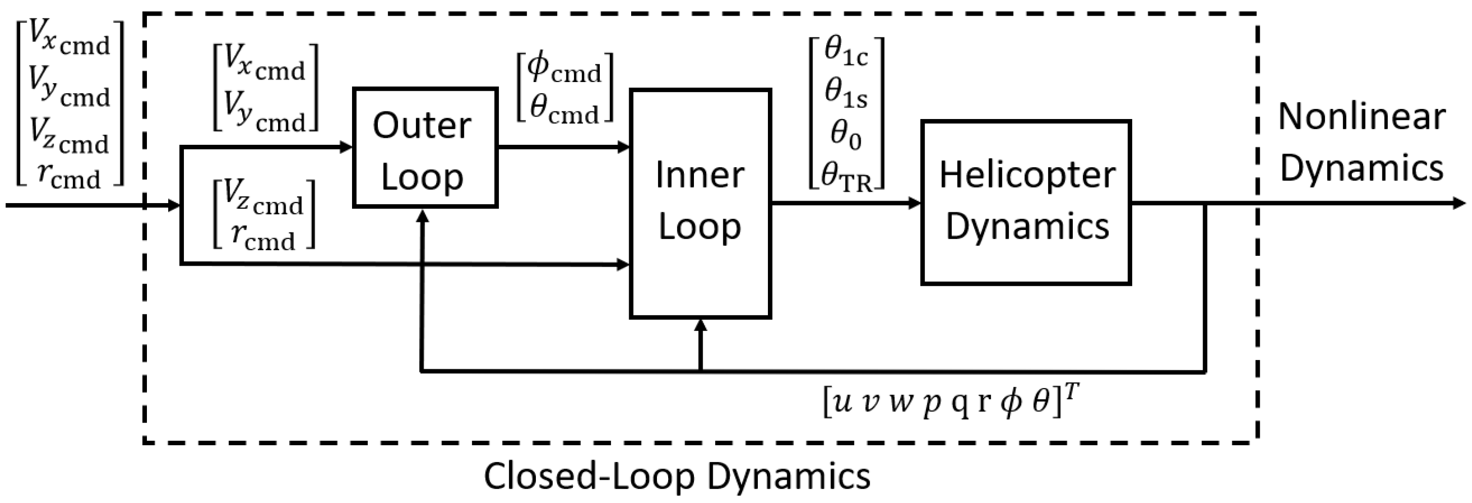
4. Autonomous Flare Control Law

A multi-loop dynamic inversion (DI) control law largely based on [12,20] is designed to enable fully autonomous flight of the helicopter in autorotation. The schematic of the closed-loop helicopter dynamics is shown in Figure 3. The outer loop controller tracks longitudinal and lateral ground velocity commands in the heading frame and calculates the desired pitch and roll attitudes for the inner loop to track. The desired response type for the outer loop is the Translational Rate Command (TRC). The inner loop achieves stability, disturbance rejection, and desired response characteristics about the roll, pitch, yaw, and heave axes. More specifically, an Attitude Command/Attitude Hold (ACAH) response is used for the roll and pitch axes, Rate Command/Attitude Hold (RCAH) is used for the yaw axis, and a TRC response is used for the heave axis. A generic DI controller applied to a linear system is shown in Figure 4. The key components are a command model (also known as command filter or reference model) that specifies desired responses to pilot commands, a feedback compensation on the tracking error, and an inner feedback loop that achieves model inversion (i.e., the feedback linearization loop).

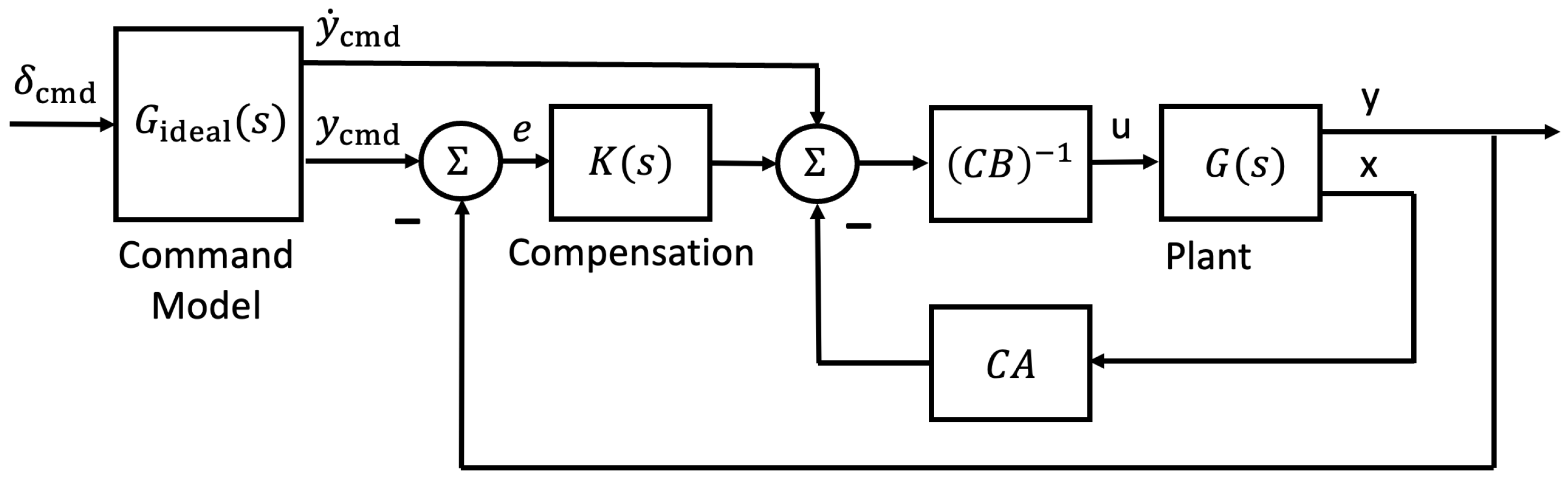
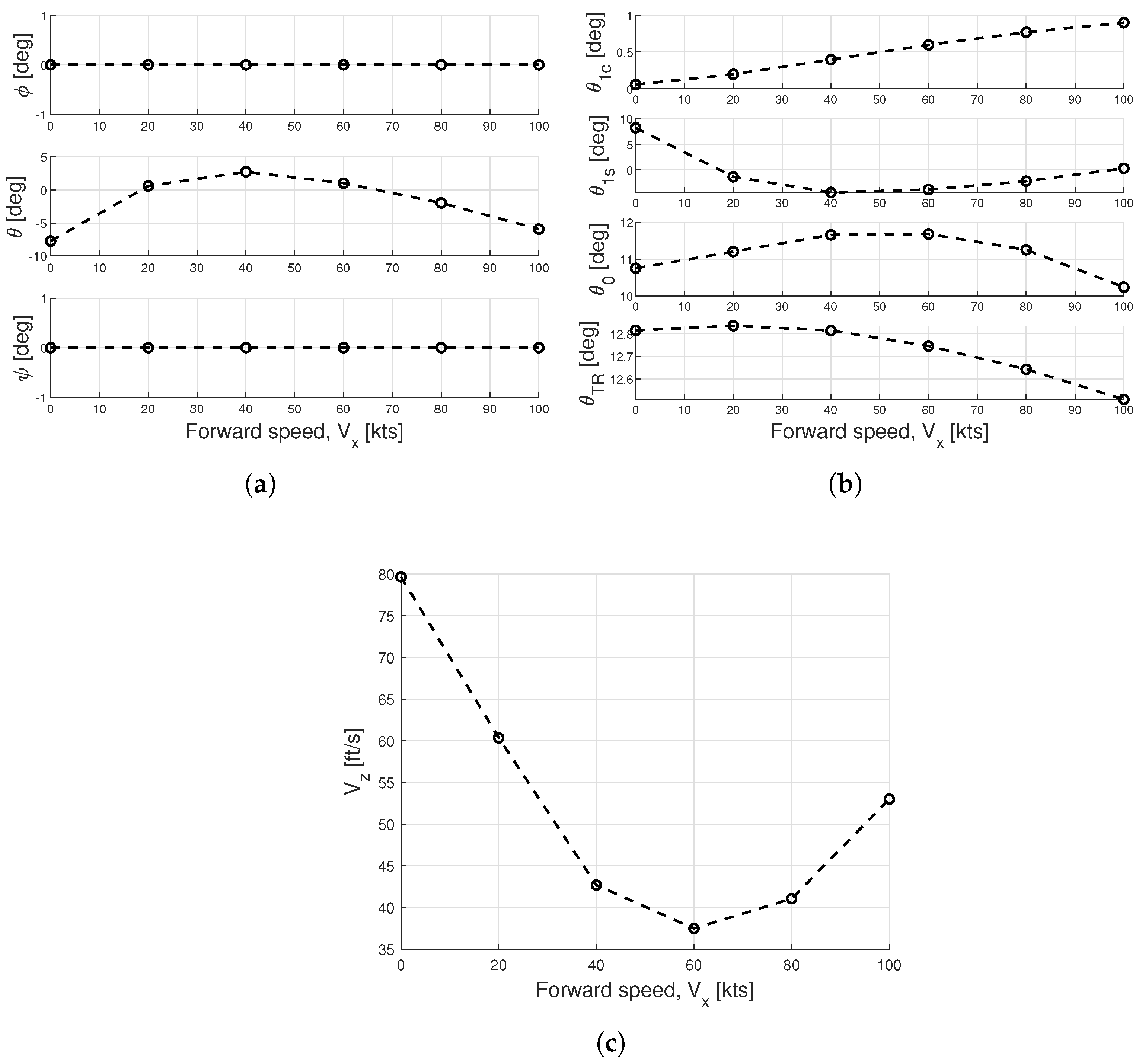
4.1. Linear Models

The first step toward the development of a DI flight control law is to obtain linear models representative of the rotorcraft flight dynamics across the flight conditions of interest. For this reason, linear models are derived by trimming the rotorcraft at incremental longitudinal speeds $V_x$ and subsequently linearizing about each trim condition:

$$\dot{\mathit{x}}=\mathit{A}\left(V_x\right)\mathit{x}+\mathit{B}\left(V_x\right)\mathit{u}$$

(6)

where the coefficient matrices $\mathit{A}$ and $\mathit{B}$ are functions of the longitudinal speed of the aircraft. Because the control law is specifically meant for an autorotative maneuver, these linear models are obtained for an autorotation condition [34,35]. That is, the trim variables are chosen as the following set of states and control inputs:

$${\mathit{x}}_{\mathrm{trim}}^T=\left[uvwpqr\varphi \theta {\theta }_{1c}{\theta }_{1s}{\theta }_0{\theta }_{0T}\right]$$

(7)

whereas the trim targets are:

$${\dot{\mathit{x}}}_{\mathrm{des}}^T=\left[\dot{u}\dot{v}\dot{w}\dot{p}\dot{q}\dot{r}\dot{\varphi }\dot{\theta }\dot{\psi }\dot{x}\dot{y}\dot{\Omega }\right]$$

(8)

All trim targets are set to zero except the derivative of the longitudinal position in the heading frame, which is set equal to the desired longitudinal speed (i.e., $\dot{x}=V_x$). Note that the vertical speed in the heading frame, $\dot{z}$, is not included in the trim targets. This is because the vertical speed is defined by the longitudinal speed $V_x$ and main rotor angular speed $\Omega$ that are assigned to the helicopter in autorotation. In autorotation, the main rotor angular speed is often chosen to be close to the nominal main rotor speed (for the UH-60, this is $\Omega =27$ rad/s) [30]. It is worth noting that, to the best knowledge of the authors, the derivation of flight control laws for the flare portion of an autorotation maneuver based on linear models derived in a steady autorotation condition has not been previously examined.

An iterative algorithm based on Newton–Rhapson is used to trim the aircraft model at incremental speeds ranging from 0 to 100 kts at intervals of 20 kts. The aircraft weight chosen for this analysis is 16,270 lb, corresponding to the piloted flight simulations discussed later in the paper. The results of this analysis are shown in Figure 5. The trim attitude across this range of speeds is shown in Figure 5a. Note that if the aircraft is trimmed with zero sideslip angle in a powered level flight, this would result in a non-zero bank angle. However, the trim bank angle in autorotation is zero because there no torque is exchanged between the main rotor and fuselage. Figure 5b shows the trim controls across the range of speeds in consideration. Notably, autorotation at low longitudinal speeds requires a high longitudinal cyclic control input. Finally, Figure 5c shows the trim vertical speed with varying longitudinal speeds. The vertical speed is shown to be minimum for a longitudinal speed equal to 60 kts. This minimum vertical speed is 37.5 ft/s, equivalent to about 2250 ft/min.

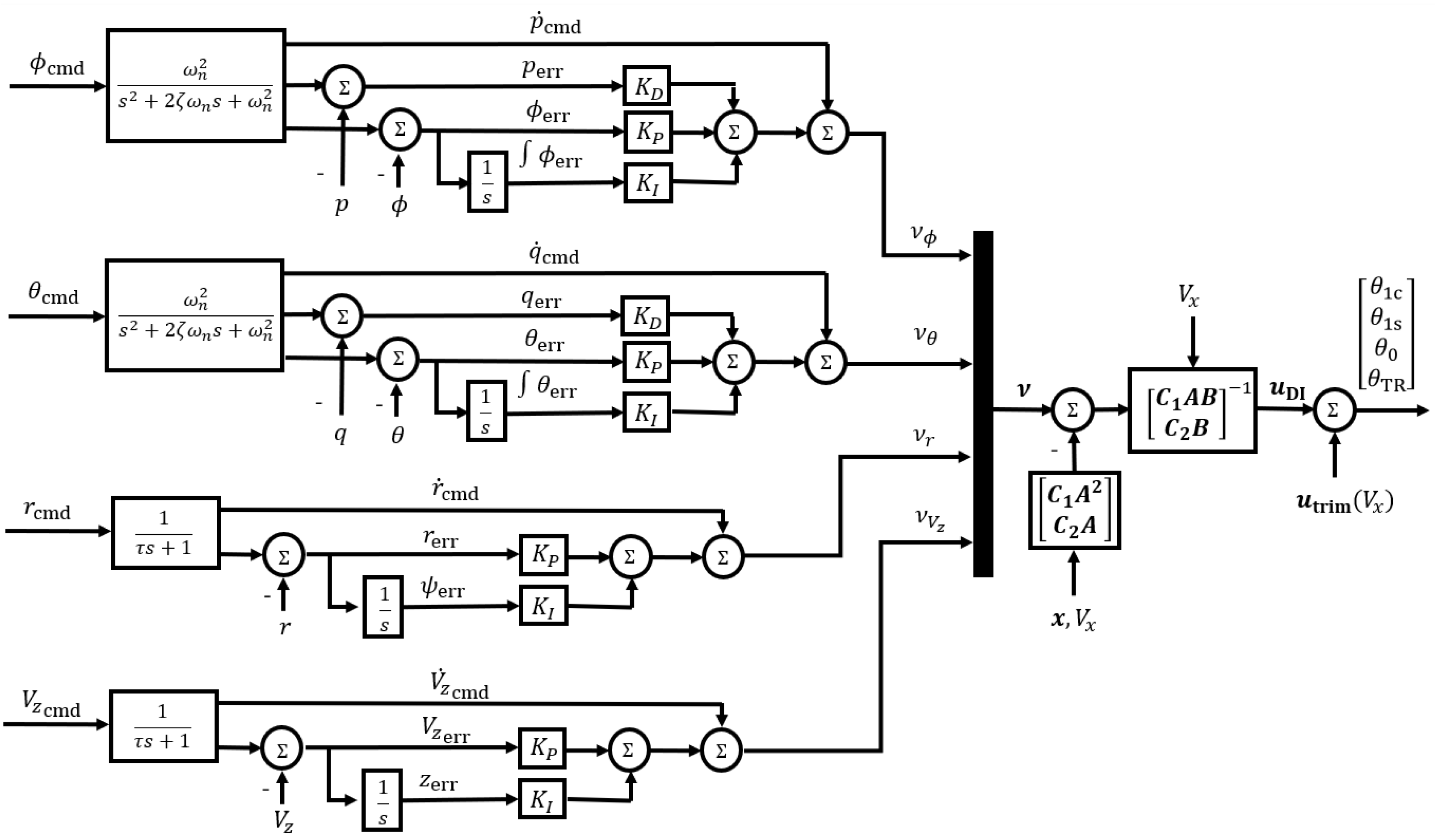
4.2. Inner Loop

To model the inner-loop DI controller, a modified state vector is defined:

$${\widehat{\mathit{x}}}^T=\left[uvwpqr\varphi \theta \right]$$

(9)

along with a modified system and control matrices $\widehat{\mathit{A}}\left(V_x\right)$ and $\widehat{\mathit{B}}\left(V_x\right)$. These modified matrices are found by truncating those rows and columns of matrices $\mathit{A}\left(V_x\right)$ and $\mathit{B}\left(V_x\right)$ corresponding to the states omitted in $\widehat{\mathit{x}}$. In addition, the following output vector is defined, corresponding to the controlled variables of the the aircraft dynamics:

$${\mathit{y}}^T=\left[\varphi \theta r{V}_z\right]$$

(10)

where $V_z$ is the vertical speed in the heading frame (positive up). The output matrix that relates the state vector to the output vector is:

$$\mathit{C}=\left[\begin{array}{c}{\mathit{C}}_1\\ {\mathit{C}}_2\end{array}\right]$$

(11)

where:

$$\begin{array}{cc}\hfill {\mathit{C}}_1& =\left[\begin{array}{cccccccc}0& 0& 0& 0& 0& 0& 1& 0\\ 0& 0& 0& 0& 0& 0& 0& 1\end{array}\right]\hfill \end{array}$$

(12a)

$$\begin{array}{cc}\hfill {\mathit{C}}_2& =\left[\begin{array}{cccccccc}0& 0& 0& 0& 0& 1& 0& 0\\ 0& 0& -1& 0& 0& 0& 0& V_x\end{array}\right]\hfill \end{array}$$

(12b)

${\mathit{C}}_1$ corresponds to the roll and pitch attitudes, whereas ${\mathit{C}}_2$ is related to the yaw rate and vertical speed. The matrix ${\mathit{C}}_2$ is a function of the longitudinal speed $V_x$ and therefore requires scheduling. This partitioning is due to the fact that the output equations for $\varphi$ and $\theta$ must be differentiated twice to have the control inputs appear explicitly in the output equation, while the same procedure only needs to be performed once for r and $V_z$:

$$\left[\begin{array}{c}\ddot{\varphi }\\ \ddot{\theta }\\ \dot{r}\\ {\dot{V}}_z\end{array}\right]=\left[\begin{array}{c}{\mathit{C}}_1{\widehat{\mathit{A}}}^2\widehat{\mathit{x}}+{\mathit{C}}_1\widehat{\mathit{A}}\widehat{\mathit{B}}\mathit{u}\\ {\mathit{C}}_2\widehat{\mathit{A}}\widehat{\mathit{x}}+{\mathit{C}}_2\widehat{\mathit{B}}\mathit{u}\end{array}\right]$$

(13)

The objective of the DI control law is that the output $\mathit{y}$ tracks a reference trajectory ${\mathit{y}}_{\mathrm{cmd}}\left(t\right)$, given by

$${\mathit{y}}_{\mathrm{cmd}}^T=\left[{\varphi }_{\mathrm{cmd}}{\theta }_{\mathrm{cmd}}{r}_{\mathrm{cmd}}{V_z}_{\mathrm{cmd}}\right]$$

(14)

with desired response characteristics. For this reason, the reference trajectory is fed through first- or second-order command models, which dictate the desired response of the system. More specifically, ${\varphi }_{\mathrm{cmd}}$ and ${\theta }_{\mathrm{cmd}}$ are fed through a second-order system, whereas $r_{\mathrm{cmd}}$ and $V_{z_{\mathrm{cmd}}}$ are fed through a first-order system. The command models are also used to extract the first and second derivatives of the filtered reference trajectory for use in the proportional–integral (PI) and proportional–integral–derivative (PID) compensators described below. The command models are of the following form:

$$\begin{array}{cc}\hfill G_{\mathrm{ideal}}^{\left(1\right)}\left(s\right)& ={\displaystyle \frac{1}{\tau s+1}}\hfill \end{array}$$

(15a)

$$\begin{array}{cc}\hfill G_{\mathrm{ideal}}^{\left(2\right)}\left(s\right)& ={\displaystyle \frac{{\omega }_n^2}{s^2+2{\omega }_n\zeta +{\omega }_n^2}}\hfill \end{array}$$

(15b)

where $\tau$ is the first-order command model time constant, which is the inverse of the command model break frequency (i.e., $\tau =1/{\omega }_n$) (note that this is not the optical Tau referred to earlier in the paper). Additionally, ${\omega }_n$ and $\zeta$ are, respectively, the natural frequency and damping ratio of the second-order command model.

Table 2. Inner loop command model parameters.

Command	${\mathit{\omega }}_{\mathit{n}}$ (Rad/s)	$\mathit{\zeta }$
Roll Attitude, $\varphi$	$4.5$	$0.7$
Pitch Attitude, $\theta$	$4.5$	$0.7$
Yaw Rate, r	$2.0$	-
Vertical Position, $V_z$	$1.0$	-

shows the values used for the parameters of the command models of the inner loop for the examples in this study.

PI and PID compensation are used to reject external disturbances and to compensate for discrepancies between the approximate model used in this derivation and the actual bare-airframe dynamics of the aircraft. The resulting DI control law is found by solving for the control vector in Equation (13), leading to:

$$\mathit{u}={\left[\begin{array}{c}{\mathit{C}}_1\widehat{\mathit{A}}\widehat{\mathit{B}}\\ {\mathit{C}}_2\widehat{\mathit{B}}\end{array}\right]}^{-1}\left(\begin{array}{c}\mathit{\nu }-\left[\begin{array}{c}{\mathit{C}}_1{\widehat{\mathit{A}}}^2\\ {\mathit{C}}_2\widehat{\mathit{A}}\end{array}\right]\widehat{\mathit{x}}\end{array}\right)$$

(16)

where $\mathit{\nu }$ is the pseudo-command vector and $\mathit{e}$ is the error as defined, respectively, in Equations (17) and (18).

$$\left[\begin{array}{c}{\nu }_{\varphi }\\ {\nu }_{\theta }\\ {\nu }_r\\ {\nu }_{V_z}\end{array}\right]=\left[\begin{array}{c}{\ddot{\varphi }}_{\mathrm{cmd}}\\ {\ddot{\theta }}_{\mathrm{cmd}}\\ {\dot{r}}_{\mathrm{cmd}}\\ {\dot{V}}_{z_{\mathrm{cmd}}}\end{array}\right]+{\mathit{K}}_P\left[\begin{array}{c}{e}_{\varphi }\\ e_{\theta }\\ e_r\\ e_{V_z}\end{array}\right]+{\mathit{K}}_D\left[\begin{array}{c}{\dot{e}}_{\varphi }\\ {\dot{e}}_{\theta }\\ 0\\ 0\end{array}\right]+{\mathit{K}}_I\left[\begin{array}{c}\int e_{\varphi }dt\\ \int e_{\theta }dt\\ \int e_{r}dt\\ \int e_{V_z}dt\end{array}\right]$$

(17)

$$\mathit{e}={\mathit{y}}_{\mathrm{cmd}}-\mathit{y};$$

(18)

The four-by-four diagonal matrices ${\mathit{K}}_P$, ${\mathit{K}}_I$, and ${\mathit{K}}_D$ identify the proportional, integral, and derivative gain matrices, respectively. Note that the coefficient matrices ${\left({\mathit{C}}_1\widehat{\mathit{A}}\widehat{\mathit{B}}\right)}^{-1}$, ${\mathit{C}}_1{\widehat{\mathit{A}}}^2$, ${\left({\mathit{C}}_2\widehat{\mathit{B}}\right)}^{-1}$, and ${\mathit{C}}_2\widehat{\mathit{A}}$ are functions of the longitudinal speed of the aircraft $V_x$. For this reason, from a practical standpoint, these matrices are computed offline at incremental longitudinal speeds from 0 to 100 kts at 20 kt intervals and stored. When the linearized DI controller is implemented on the nonlinear aircraft dynamics, the coefficient matrices ${\left({\mathit{C}}_1\widehat{\mathit{A}}\widehat{\mathit{B}}\right)}^{-1}$, ${\mathit{C}}_1{\widehat{\mathit{A}}}^2$, ${\left({\mathit{C}}_2\widehat{\mathit{B}}\right)}^{-1}$, and ${\mathit{C}}_2\widehat{\mathit{A}}$ are computed at each time step via interpolation based on the current longitudinal airspeed $V_x\left(t\right)$ and on the lookup tables stored offline. It is important to note that what is implemented on the nonlinear aircraft dynamics is linearized DI. However, because the coefficient matrices are scheduled with the longitudinal speed, where scheduling effectively introduces a nonlinear relation between the aircraft states and the feedback control input, the controller implemented is effectively nonlinear DI [17]. It is also worth noting that, as discussed in [17], DI has issues when the plant model used for control design shows transmission zeros in the right-half of the complex plane, i.e., non-minimum phase (NMP) zeros. Clearly, when a transfer function with NMP zeros is inverted, it has unstable poles. Similarly, it is well known that the inversion in DI will also produce unstable modes corresponding to NMP zeros of the open-loop plant model. For typical rotorcraft dynamics, multiple NMP zeros are quite prevalent in the full-order dynamics but less common in the reduced-order rigid body models used for DI control design. When NMP zeros do occur in the reduced-order models, they are generally benign (as they are small in magnitude and thus at low frequency) and can be handled through minor modifications to controlled variables [36] or through outer control loops. A block diagram of the linearized DI flight control law is shown in Figure 6.

To ensure that the control inputs respect the maximum and minimum swashplate and tail rotor control inputs allowed by the UH-60 platform, the control inputs from the autonomous flare control law are saturated according to the specifications found in [30]. The control input ranges are reported in

Table 3. Swashplate and tail rotor control input range for UH-60 helicopter.

Control Input	Min. (deg)	Max. (deg)
Lateral Cyclic, ${\theta }_{1c}$	−7	7
Longitudinal Cyclic, ${\theta }_{1s}$	−12	12
Collective, ${\theta }_0$	6.5	22.5
Tail Rotor Collective, ${\theta }_{0T}$	−6	25

.

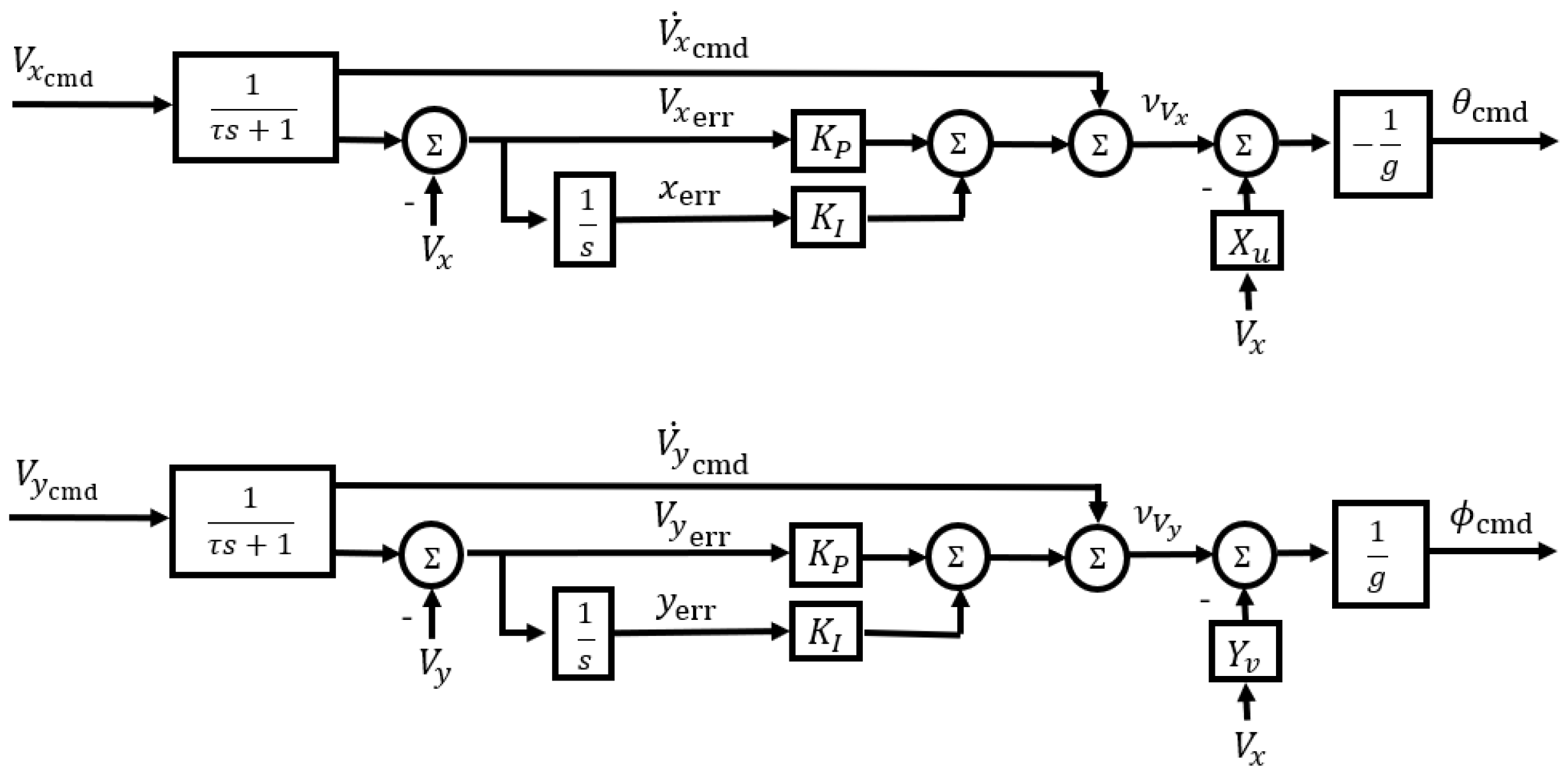
4.3. Outer Loop

The objective of the outer loop is to track longitudinal and lateral velocities in the heading frame, such that the reference trajectory is given by:

$${\mathit{y}}_{\mathrm{cmd}}^T=\left[V_{x_{\mathrm{cmd}}}{V}_{y_{\mathrm{cmd}}}\right]$$

(19)

The heading frame is a vehicle-carried frame where the x-axis is aligned with the current aircraft heading, the z-axis is positive up in the inertial frame, and the y-axis points to the right, forming a left-handed orthogonal coordinate system. The following equation shows the rotation from the body to the heading frame:

$${\mathit{T}}_{h/b}=\left[\begin{array}{ccc}cos\theta & sin\varphi sin\theta & cos\varphi sin\theta \\ 0& cos\varphi & -sin\varphi \\ sin\theta & -sin\varphi cos\theta & -cos\varphi cos\theta \end{array}\right]$$

(20)

such that the velocities in the heading frame are given by:

$$\left[\begin{array}{c}{V}_x\\ V_y\\ V_z\end{array}\right]={\mathit{T}}_{h/b}\left[\begin{array}{c}u\\ v\\ w\end{array}\right]$$

(21)

The following approximate model of the longitudinal and lateral dynamics of the helicopter is used to derive the outer loop control law:

$$\underset{\dot{\widehat{\mathit{x}}}}{\underbrace{\left[\begin{array}{c}{\dot{V}}_x\\ {\dot{V}}_y\end{array}\right]}}=\underset{\widehat{\mathit{A}}}{\underbrace{\left[\begin{array}{cc}{X}_u& 0\\ 0& Y_v\end{array}\right]}}\underset{\widehat{\mathit{x}}}{\underbrace{\left[\begin{array}{c}{V}_x\\ V_y\end{array}\right]}}+\underset{\widehat{\mathit{B}}}{\underbrace{\left[\begin{array}{cc}-g& 0\\ 0& g\end{array}\right]}}\underset{\mathit{u}}{\underbrace{\left[\begin{array}{c}\theta \\ \varphi \end{array}\right]}}$$

(22a)

$$\underset{\mathit{y}}{\underbrace{\left[\begin{array}{c}x\\ y\end{array}\right]}}=\underset{\mathit{C}}{\underbrace{\left[\begin{array}{cccc}0& 1& 0& 0\\ 0& 0& 0& 1\end{array}\right]}}\underset{\widehat{\mathit{x}}}{\underbrace{\left[\begin{array}{c}{V}_x\\ x\\ V_y\\ y\end{array}\right]}}$$

(22b)

where $\widehat{\mathit{x}}$ is the modified state vector, and $\widehat{\mathit{A}}\left(V_x\right)$ and $\widehat{\mathit{B}}$ are the modified system and control matrices. Note that these modified quantities are different from those used in the inner loop control design. The stability derivatives in the system matrix are scheduled with flight speed. The control matrix is not scheduled with speed as it is only composed of zeros and gravitational acceleration (i.e., g). The output matrix $\mathit{C}$ is also not scheduled with speed as it is composed solely of ones and zeros. The command models for the longitudinal and lateral speeds are first order. The natural frequencies and damping ratios are given in

Table 4. Outer loop command model parameters.

Command	${\mathit{\omega }}_{\mathit{n}}$ (Rad/s)	$\mathit{\zeta }$
Longitudinal Speed, $V_x$	1	0.7
Lateral Speed, $V_y$	1	0.7

.

Following a similar procedure to the inner loop yields an outer loop control law of the form:

$$\mathit{u}={\left(\mathit{C}\widehat{\mathit{A}}\widehat{\mathit{B}}\right)}^{-1}\left(\mathit{\nu }-\mathit{C}{\widehat{\mathit{A}}}^2\widehat{\mathit{x}}\right)$$

(23)

The reference trajectory is subtracted from the output to find the error, which is compensated by a PI controller. The feed-forward signal is subsequently added, leading to the pseudo-control vector for the outer loop:

$$\left[\begin{array}{c}{\nu }_x\\ {\nu }_y\end{array}\right]=\left[\begin{array}{c}{\dot{V}}_{x_{\mathrm{cmd}}}\\ {\dot{V}}_{y_{\mathrm{cmd}}}\end{array}\right]+{\mathit{K}}_P\left[\begin{array}{c}{e}_x\\ e_y\end{array}\right]+{\mathit{K}}_I\left[\begin{array}{c}\int e_{x}dt\\ \int e_{y}dt\end{array}\right]$$

(24)

The DI outer loop block diagram is shown in Figure 7.

During flare, the helicopter decelerates from relatively high-speed flight (i.e., greater than 60 kts) to low-speed flight (i.e., lower than 40 kts); therefore, different control strategies are needed to control the yaw rate. Above 60 kts, turn coordination is used; below 40 kts, no turn coordination [37] is used; between 40 and 60 kts, a blend between the two is used. These three control strategies are summarized as follows:

$$r_{\mathrm{cmd}}^{\prime }=\left\{\begin{array}{cc}{r}_{\mathrm{cmd}}\hfill & V<V_{\mathrm{LS}}\hfill \\ r_{\mathrm{cmd}}+{\displaystyle \frac{g}{V}}sin\varphi \left({\displaystyle \frac{V-V_{\mathrm{LS}}}{V_{\mathrm{HS}}-V_{\mathrm{LS}}}}\right)\hfill & V_{\mathrm{LS}}\le V<V_{\mathrm{HS}}\hfill \\ r_{\mathrm{cmd}}+{\displaystyle \frac{g}{V}}sin\varphi \hfill & V\ge V_{\mathrm{HS}}\hfill \end{array}\right.$$

(25)

where $V=\sqrt{V_x^2+V_y^2+V_z^2}$ is the total speed of the aircraft, $V_{\mathrm{LS}}=40$ kts, and $V_{\mathrm{HS}}=60$ kts.

To model the final pushover maneuver to level the rotorcraft before contact to the ground, the outer loop of the DI flight control law described above requires modification. To induce a pushover prior to touchdown so that the helicopter lands with an acceptable pitch attitude, the pitch attitude command for tail wheel altitudes less than 6 ft is set to 0 deg. This pitch attitude command effectively bypasses the pitch attitude command from the outer-velocity loop when $h_{\mathrm{TW}}\le 6$ ft. This ensures the helicopter pitches over before making contact with the ground, especially when descending at high pitch attitudes in the final stages of the flare maneuver. Thus, the pitch attitude command to the inner loop is given by:

$${\theta }_{\mathrm{cmd}}^{\prime }=\left\{\begin{array}{cc}{\theta }_{\mathrm{cmd}}\hfill & h_{\mathrm{TW}}>6\mathrm{ft}\hfill \\ 0\hfill & h_{\mathrm{TW}}\le 6\mathrm{ft}\hfill \end{array}\right.$$

(26)

4.4. Error Dynamics

Feedback compensation is needed to ensure the system tracks the command models. It can be demonstrated [38] that for a DI control law, the output equation must be differentiated n times for the controls to appear explicitly in the output equation:

$$e^{\left(n\right)}=y_{\mathrm{cmd}}^{\left(n\right)}-\nu$$

(27)

For output equations that require differentiation only once, a PI control strategy is applied to the pseudo-command vector:

$$\nu ={\dot{y}}_{\mathrm{cmd}}\left(t\right)+K_{P}e\left(t\right)+K_I{\int }_0^{t}e\left(\tau \right)d\tau$$

(28)

Substituting Equation (28) into Equation (27) leads to the closed-loop error dynamics:

$$\dot{e}\left(t\right)+K_{P}e\left(t\right)+K_I{\int }_0^{t}e\left(\tau \right)d\tau =0$$

(29)

The gains are chosen such that the frequencies of the error dynamics are of the same order as the command filters (i.e., first order), ensuring that the bandwidth of the response to disturbances is comparable to that of an input given by a pilot or outer loop. By taking the Laplace transform, and therefore switching to the frequency domain, the error dynamics become:

$$e\left(s\right)\left(s^2+s{K}_P+K_I\right)=0$$

(30)

To obtain the gains that guarantee the desired response, the error dynamics of Equation (30) are set equal to the following second-order system:

$$s^2+2\zeta {\omega }_{n}s+{{\omega }_n}^2=0$$

(31)

yielding the following proportional and integral gains:

$$\begin{array}{c}\hfill K_P=2\zeta {\omega }_n\end{array}$$

(32a)

$$\begin{array}{c}\hfill K_I={{\omega }_n}^2\end{array}$$

(32b)

Similarly, for those outputs that must be differentiated twice, a PID control strategy is applied to the pseudo-command vector:

$$\nu ={\ddot{y}}_{\mathrm{cmd}}\left(t\right)+K_D\dot{e}\left(t\right)+K_{P}e\left(t\right)+K_I{\int }_0^{t}e\left(\tau \right)d\tau$$

(33)

Substituting Equation (33) into Equation (27) leads to the following closed-loop error dynamics:

$$\ddot{e}\left(t\right)+K_D\dot{e}\left(t\right)+K_{P}e\left(t\right)+K_I{\int }_0^{t}e\left(\tau \right)d\tau =0$$

(34)

and, therefore, to:

$$e\left(s\right)\left(s^3+K_D{s}^2+K_{P}s+K_I\right)=0$$

(35)

Again, the gains are chosen such that the frequencies of the error dynamics are of the same order as the command filters (i.e., second order), ensuring that the bandwidth of the response to disturbances is comparable to that of an input given by a pilot or outer loop. To obtain the gains that guarantee the desired response, the error dynamics of Equation (35) are set equal to the following third-order system:

$$(s^2+2\zeta {\omega }_{n}s+{{\omega }_n}^2)(s+p)=0$$

(36)

yielding the following proportional, integral, and derivative gains:

$$\begin{array}{c}{K}_D=2\zeta {\omega }_n+p\end{array}$$

(37a)

$$\begin{array}{c}{K}_P=2\zeta {\omega }_{n}p+{{\omega }_n}^2\end{array}$$

(37b)

$$\begin{array}{c}{K}_I={{\omega }_n}^{2}p\end{array}$$

(37c)

This compensation strategy is used to ensure trajectory tracking in both the inner and outer loops.

Table 5. Inner loop disturbance rejection natural frequencies, damping ratios, and integrator poles.

	${\mathit{\omega }}_{\mathit{n}}$ (Rad/s)	$\mathit{\zeta }$	p
${\varphi }_{\mathrm{cmd}}$	4.5	0.7	0.75
${\theta }_{\mathrm{cmd}}$	4.5	0.7	0.75
$r_{\mathrm{cmd}}$	2	0.7	-
$V_{z_{\mathrm{cmd}}}$	1	0.7	-

and

Table 6. Outer loop disturbance rejection natural frequencies and damping ratios.

	${\mathit{\omega }}_{\mathit{n}}$ (Rad/s)	$\mathit{\zeta }$
$V_{x_{\mathrm{cmd}}}$	1	0.7
$V_{y_{\mathrm{cmd}}}$	1	0.7

show the natural frequencies, damping ratios, time constants, and the integrator pole values, respectively, for the inner and the outer loops of the examples in this study. Note that the integrator pole p is usually chosen to be one-fifth of the natural frequency, corresponding to about one-fifth of the loop crossover frequency [39]. Further, the outer loop error dynamics natural frequency must be $1/10$ to $1/5$ of the inner loop error dynamics’ natural frequency to ensure sufficient frequency separation [39]. Additionally, because the plant is inverted in the feedback linearization loop such that the system being controlled is effectively a set of integrators, there is no need for gain scheduling. However, the plant model used for feedback linearization must still be scheduled with the flight condition (i.e., with $V_x$ in this case).

Table 7. Inner loop compensation gains.

	${\mathit{K}}_{\mathit{P}}$	${\mathit{K}}_{\mathit{I}}$	${\mathit{K}}_{\mathit{D}}$
${\varphi }_{\mathrm{cmd}}$	24.975	15.1875	7.05
${\theta }_{\mathrm{cmd}}$	24.975	15.1875	7.05
$r_{\mathrm{cmd}}$	4	4	4
$V_{z_{\mathrm{cmd}}}$	2	1	-

and

Table 8. Outer loop compensation gains.

	${\mathit{K}}_{\mathit{P}}$	${\mathit{K}}_{\mathit{I}}$
$V_{x_{\mathrm{cmd}}}$	1.5	0.5625
$V_{y_{\mathrm{cmd}}}$	1.5	0.5625

show the compensation gains for the inner and outer loops used in the simulation results presented here.

5. Results

5.1. Demonstration of Autonomous Flare Control Law

To demonstrate the methodology, simulation results are compared to piloted flight simulations for the case of a flare maneuver initiated at 80 kts total speed, at a downrange target landing distance of 1000 ft from the autorotation initiation point, for a flare entry altitude of 140 ft. While Figure 5c shows that the speed for minimum descent rate is 60 kt, it was found in piloted simulations [33,40,41] that this speed left very little energy for the flare at the end of the maneuver. Thus, 80 kts was chosen as initial speed. The gross weight of the UH-60 is set as 16,270 lb. Piloted flight simulations were performed using the fully reconfigurable research HELIFLIGHT-R flight simulator operated by the University of Liverpool [42]. Fourteen autorotation maneuvers were performed by the Test Pilot who is an ex-Royal Navy rotary wing pilot and a graduate of the UK’s Empire Test Pilot School (ETPS). These piloted simulations are shown in Figure 8, taken from [33,40,41]. Note that the piloted flight simulations were performed using FLIGHTLAB^TM, a mid-fidelity flight dynamics model [43]. The pilot was tasked to initiate the flare at 80 kts and at altitudes between 150 and 200 ft. Each run is represented with different colors. Figure 8a shows the longitudinal and vertical speeds at which the flare maneuvers are initiated. It can be seen that the longitudinal speed at the entry to the flare is between 65 and 80 kts. The vertical speed varies approximately between $-40$ and $-25$ ft/s. The variation of vertical speed at the entry to flare depends on the longitudinal speed. For example, when the pilot enters the flare with a higher longitudinal speed, the vertical speed is lower. Figure 8b shows longitudinal position and altitude trajectories. Downrange distances at which flare is initiated vary from approximately 850 to 1150 ft, whereas initial altitudes span between 120 to 190 ft. Figure 8c shows rotor speed, collective pitch input, and pitch attitude time histories. This figure suggests a trend in which pushover is initiated at about 3 to 5 s prior to touchdown.

The duration of the flare maneuver used in trajectory generation is chosen as the average time elapsed between the initiation of flare and touchdown as observed in the piloted simulations, which is 12 s. To compare the pilot’s flare strategy with that from the proposed method, parameters of the piloted simulations are averaged at each time step over the 12 s preceding touchdown. Comparison results are shown in Figure 9. Figure 9a shows the longitudinal and vertical velocity trajectories generated with Tau theory (dashed red line). These trajectories result in the optimal parameters $k_{{\mathrm{opt}}_1}=0.3387$ and $k_{{\mathrm{opt}}_2}=0.7315$. This figure also shows excellent tracking of the tau-generated trajectories by the closed-loop helicopter model up until the pushover. When the pushover is initiated, because of the proximity of the helicopter tail wheel to the ground, longitudinal velocity tracking is effectively no longer enforced as pitch angle is commanded directly to the controller inner loop. This causes the longitudinal speed to remain approximately constant after the initiation of the pushover maneuver. Notably, the pilot appears to decelerate more gradually in the initial stages of the flare. However, the longitudinal speed at touchdown is similar for the piloted and autonomous simulations (i.e., approximately 20 kts). It is also worth noting that the lateral speed for the autonomous simulation remains approximately zero throughout the flare maneuver, which indicates good off-axis disturbance rejection from the NDI control law. Figure 9b shows the longitudinal position and altitude of the helicopter. In this figure, it is shown that longitudinal position and altitude trajectories from piloted and autonomous simulations are very similar, indicating the potential validity of the proposed approach. As shown in Figure 9c, pushover is initiated by the pilot at approximately 8 s into flare, whereas the autonomous control law delays pushover to the ninth second. Despite this difference, pitch attitudes at touchdown are similar, approximately 10 deg. In this figure, it is also shown that the roll and yaw angle magnitudes in the autonomous flare case remain small, which, again, indicates good performance of the controller in mitigating the off-axis response.

Finally, Figure 9d shows the time histories for the main rotor angular speed and collective angle. These variables follow the trend of typical flare maneuvers, where the main rotor angular speed first increases due to the increase in inflow from the pitch up, and then decreases as the rotor trades kinetic energy to decelerate the vehicle. Similarly, the main rotor collective angle increases gradually at the beginning of the flare to reduce the vertical speed, and increases more rapidly during the pushover. These results suggest that a control law based on linearized models obtained in steady-state autorotation, in conjunction with a trajectory generation algorithm based on optical Tau theory, is suitable for performing autonomous flare maneuvers in helicopter autorotation. More specifically, trajectories generated with optical Tau theory are shown to be similar to those employed by pilots in flare maneuvers, whereas the NDI control law is shown to accurately track these trajectories in this example case.

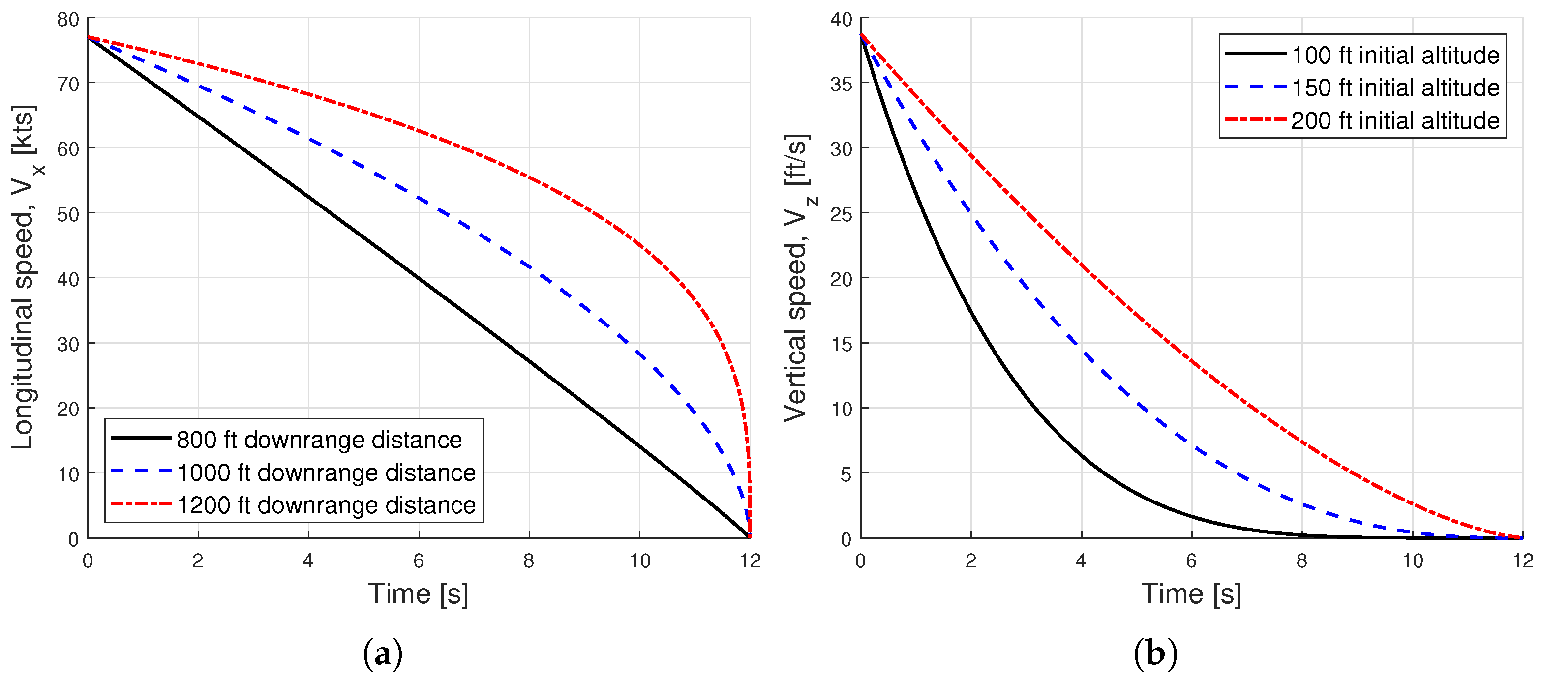
5.2. Reachability Study

Because the NDI controller is capable of performing autonomous autorotative flare maneuvers, it can be used as a tool to determine which combinations of downrange distances and altitudes at flare entry result in a successful landing. Touchdown performance is measured by comparing critical rotorcraft state touchdown parameters against guideline metrics for desired and adequate touchdown in [31] and is reported in

Table 9. Conditions for successful and marginal autorotative landings.

	${\mathit{V}}_{\mathit{x}}$ (ft/s)	${\mathit{V}}_{\mathit{z}}$ (ft/s)	$\mathit{\theta }$ (deg)	q (deg/s)	$\mathbf{\Omega }/{\mathbf{\Omega }}_0$ (%)
Successful	$<30$	$<-8$	$<12$	$-30\mathrm{to}20$	$90\mathrm{to}110$
Marginal	$<60$	$<-15$	$<20$	$-50\mathrm{to}40$	$80\mathrm{to}120$

. This table also includes bounds on the angular speed of the main rotor, which is not only evaluated at touchdown but throughout the flare maneuver. Minimum rotor speed is evaluated only until pushover.

A parametric study was conducted in which flare maneuvers were simulated for varying downrange distances of the intended landing point and altitudes at flare entry. Downrange distances varied from 800 to 1200 ft from the flare initiation point in increments of 20 ft, whereas altitudes at flare entry varied between 100 and 200 ft in increments of 10 ft. These ranges were chosen based on indications from previous studies [44] involving piloted simulations, and on the piloted simulation data described above. Flare maneuvers were initiated at 80 kts total speed and at an aircraft weight of 16,270 lbs so as to be consistent with the parameters used in the piloted simulations. Figure 10 shows the critical aircraft state parameters for those flare maneuvers simulated as part of this parametric study. Figure 10a shows that the longitudinal speed at touchdown tends to be higher for high downrange distances and low altitudes at flare entry. This is because, as shown in Figure 2a, the deceleration in longitudinal speed for high downrange distances is concentrated at the end of the trajectory. As such, the helicopter has limited time and altitude to slow down before it pitches over just before touchdown. The premature pitch-over causes the longitudinal deceleration to be cut short, and thus the forward speed remains relatively high. Figure 10b shows that the vertical speed at touchdown is within the adequate bounds for most of the downrange distances and altitudes considered, except for low altitudes and downrange distances at flare entry. Figure 10c shows that low altitudes at flare entry generally result in low pitch attitudes at touchdown. On the other hand, low downrange distances and high altitudes result in higher pitch angles at touchdown. Figure 10d shows that pitch rate at touchdown is largely within the desired boundaries. Figure 10e shows that minimum rotor speed requirements are met for all conditions. On the other hand, maximum desired rotor speed limits are exceeded for low downrange distances and high flare initiation altitudes, as shown in Figure 10f.

Based on the results from the parametric study, combinations of downrange distances and altitudes at flare initiation that present successful and marginal landings are shown in Figure 11. In this figure, conditions for successful touchdown are marked in black, whereas those for marginal touchdown are marked in gray. Successful autorotation for the flight condition under consideration (80 kts total speed and aircraft weight of 16,270 lb) is achieved for downrange distances of 920–1150 ft and flare initiation altitudes of 130–180 ft. Successful and marginal piloted autorotations, still evaluated with the criteria in Table 9, are overlaid on the reachability plot obtained from autonomous flares. Although two successful piloted autorotations were performed for conditions that resulted in marginal landings in autonomous simulations, most successful autorotations fall within the successful bounds predicted using the autonomous control law. Half of the marginal piloted landings fell within the successful bounds for the autonomous control law, while half fell within the marginal bounds. These results raise the possibility that the autonomous control law can land the aircraft with improved touchdown parameters more reliably from favorable initial conditions compared to human pilots.

6. Conclusions

A novel trajectory generation and control architecture for fully autonomous autorotation flare that combines rapid path generation with model-based control was proposed. The trajectory generation component uses optical Tau theory to rapidly compute flare trajectories for both longitudinal and vertical speeds. These flare trajectories are tracked using a nonlinear dynamic inversion (NDI) control law scheduled with linear systems obtained in steady-state autorotation at varying speeds. Computer simulations were used to demonstrate that the NDI control law is able to successfully execute an autorotative flare for a simulated UH-60 aircraft. Simulations of the autonomous flare algorithm are compared with piloted simulation data to assess the similarities and/or discrepancies between the autonomous flare strategies and those used by a pilot. Trade studies examine the combinations of downrange distances and altitudes at flare initiation that result in successful and marginal autorotative landings. Based on this work, the following conclusions can be drawn:

• Scheduling of the NDI control law with linearized models of the rotorcraft flight dynamics in steady-state autorotation has been shown to be a successful approach for tracking flare trajectories. In addition to achieving adequate tracking of the longitudinal and vertical trajectories, the control law also showed good performance in mitigating the off-axis response.
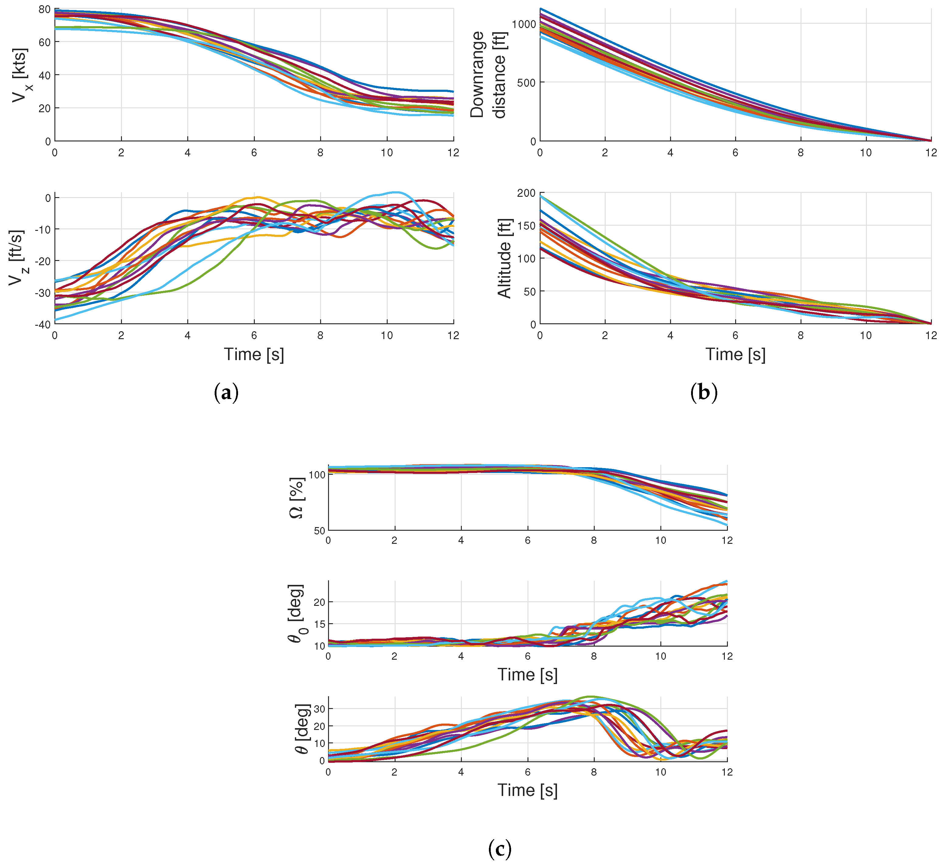
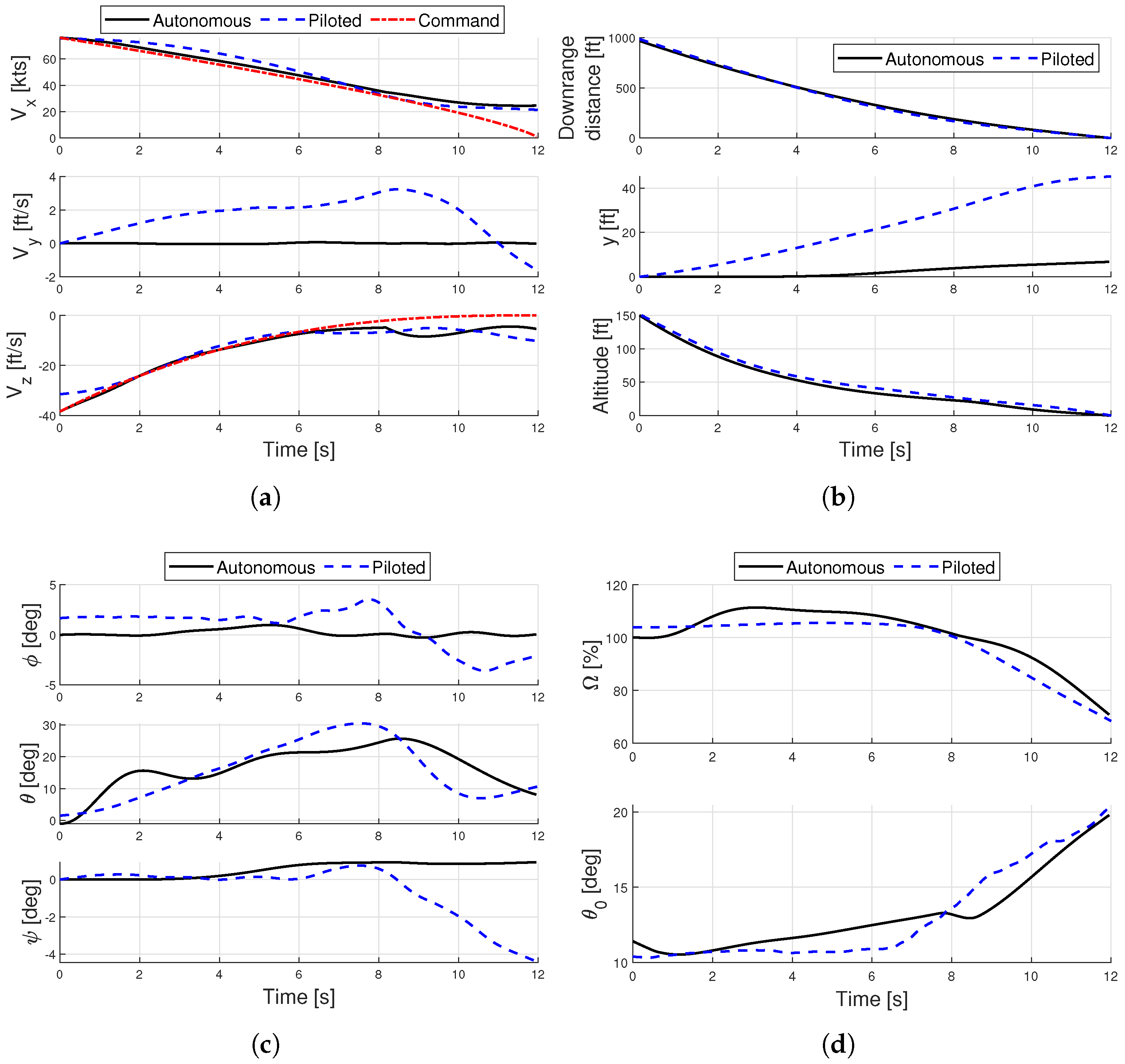
• State histories of the autonomous flare maneuvers largely mimic those of piloted flight simulations. Noticeable differences lie in a more aggressive longitudinal deceleration in the early stages of flare, and a delayed pitchover before landing.
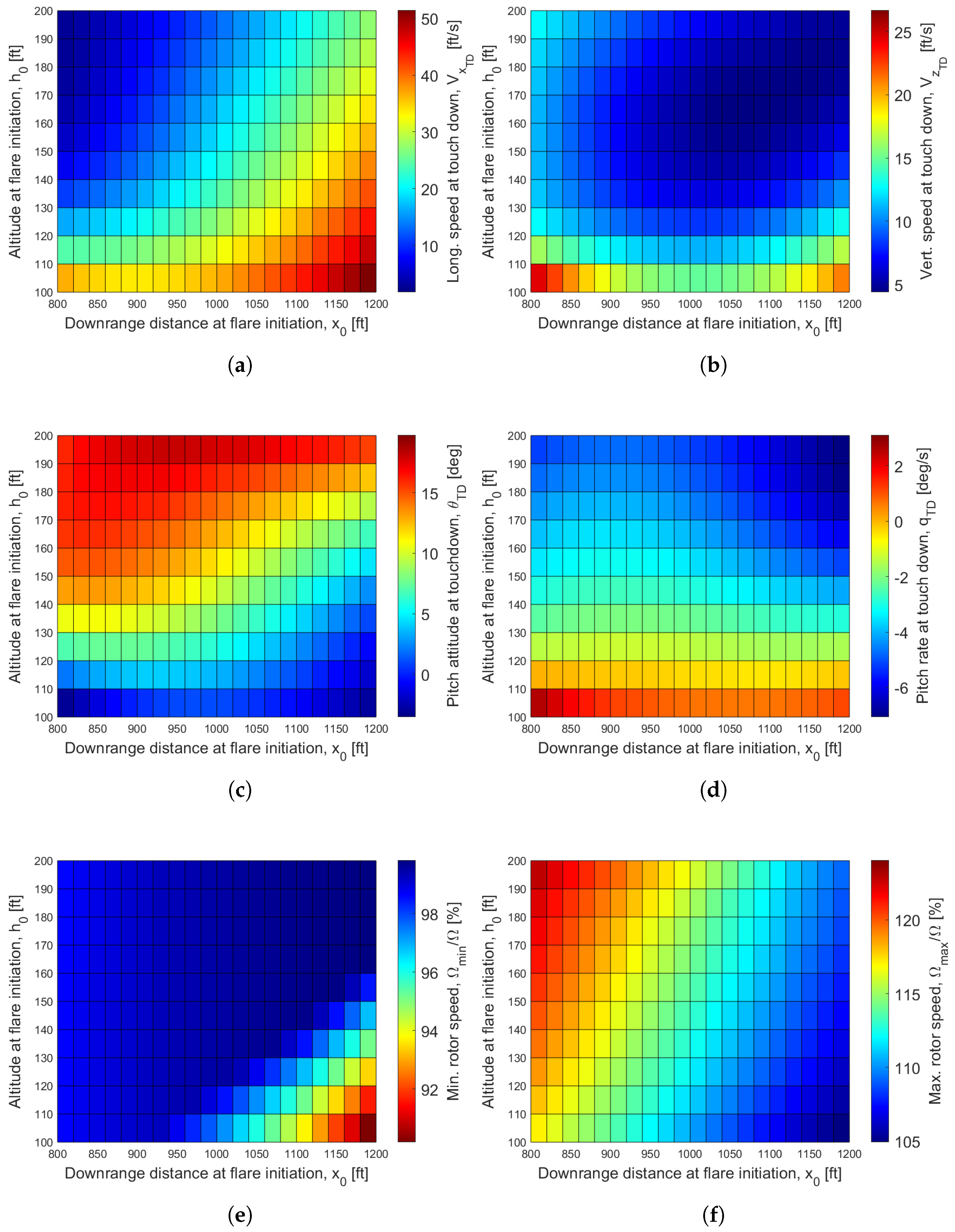
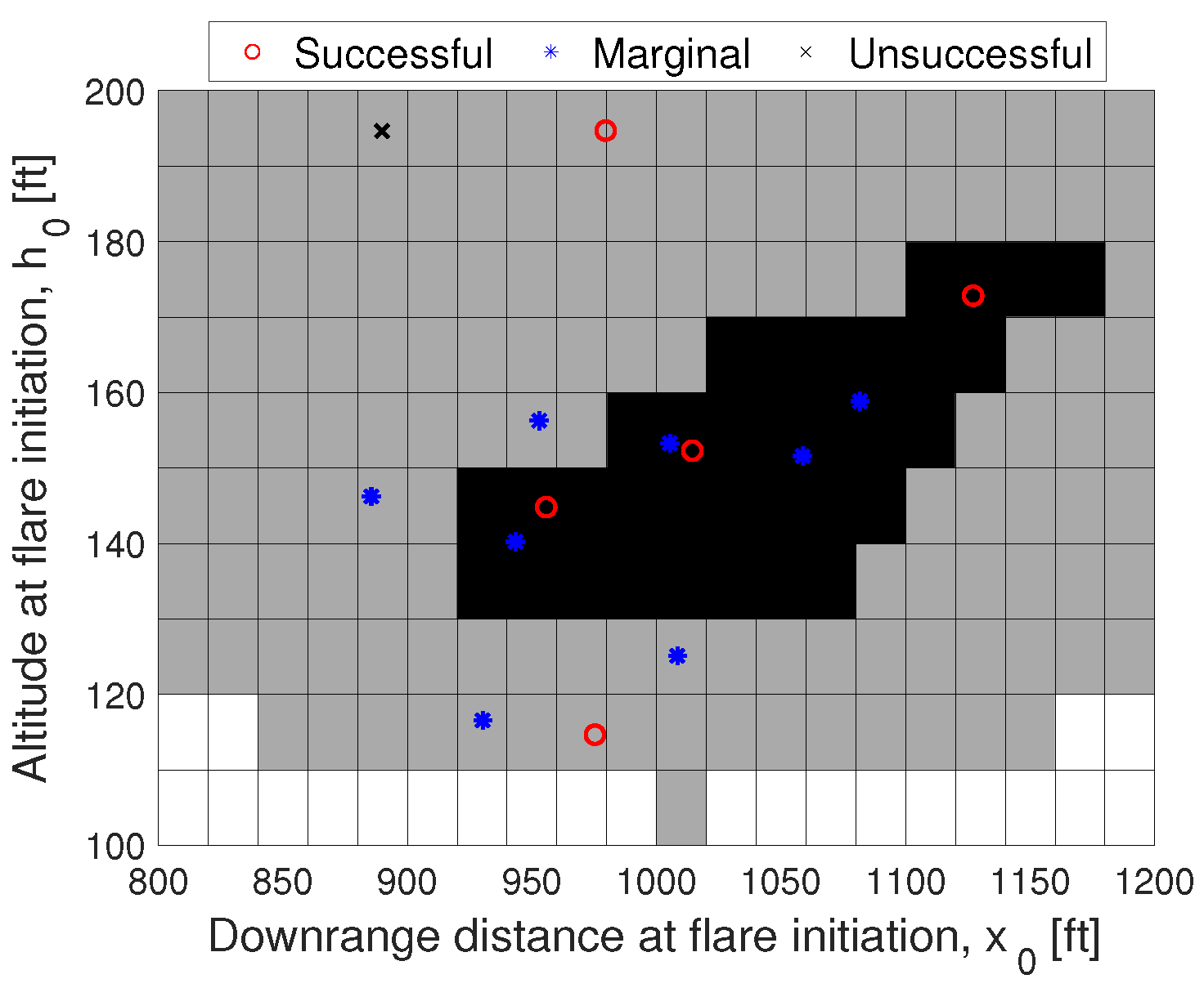
• The proposed method was used to predict combinations of downrange distances and altitudes at flare entry that result in desired and marginal landings. These predictions are in line with piloted flight simulation data, suggesting that the method may be used not only for real-time control, but also potentially for reachability predictions in the autorotation flare.

While the proposed method is demonstrated for a conventional main-tail rotor helicopter configuration, it is potentially applicable to other rotorcraft configurations like Future Vertical Lift (FVL) or Urban Air Mobility (UAM) configurations. FVL configurations include winged single main rotor (wSMR), lift-offset coaxial (LOC), and tiltrotor configurations [45,46,47], whereas UAM configurations are highly diverse. Attempts to categorize the various UAM configurations are provided in [48,49]. The trajectory generation component of the proposed method is broadly transferable as it is model agnostic. On the other hand, modifications to the NDI control law may be necessary depending on the configuration of interest. For instance, NDI flight control laws for tiltrotors or coaxial compound helicopters can be adapted through [50,51], whereas NDI flight control laws for lift+cruise UAM vehicles can be based on [52].

References

- Sunberg, Z.N.; Miller, N.R.; Rogers, J.D. A Real-Time Expert Control System For Helicopter Autorotation. J. Am. Helicopter Soc. 2015, 60, 1–15. [Google Scholar] [CrossRef][Green Version]
- Bachelder, E.N.; Aponso, B.L. Using Optimal Control for Rotorcraft AutorotationTraining. In Proceedings of the 59th Annual Forum of the American Helicopter Society, Phoenix, AZ, USA, 6–8 May 2003. [Google Scholar]
- Aponso, B.L.; Lee, D.; Bachelder, E.N. Evaluation of a Rotorcraft Autorotation Training Display on a Commercial Flight Training Device. J. Am. Helicopter Soc. 2007, 52, 123–133. [Google Scholar] [CrossRef]
- Keller, J.D.; McKillip, R.; Horn, J.F.; Yomchinda, T. Active Flight Control and Appliqué Inceptor Concepts for Autorotation Performance Enhancement. In Proceedings of the 67th Annual Forum of the American Helicopter Society, Virginia Beach, VA, USA, 3–5 May 2011. [Google Scholar]
- Rogers, J.; Repola, L.; Jump, M.; Cameron, N.; Fell, T. Handling Qualities Assessment of a Pilot Cueing System for Autorotation Maneuvers. In Proceedings of the 73rd Annual Forum of the American Helicopter Society, Fort Worth, TX, USA, 9–11 May 2017. [Google Scholar]
- Yomchinda, T. Real-Time Path Planning and Autonomous Control for Helicopter Autorotation. Ph.D. Thesis, Pennsylvania State University, University Park, PA, USA, 2013. [Google Scholar]
- Yomchinda, T.; Horn, J.; Langelaan, J. Flight Path Planning for Descent-phase Helicopter Autorotation. In Proceedings of the AIAA Guidance, Navigation and Control Conference, Portland, OR, USA, 8–11 August 2011. [Google Scholar]
- Grande, N.; Tierney, S.; Horn, J.; Langelaan, J. Safe Autorotation Through Wind Shear Via Backward Reachable Sets. J. Am. Helicopter Soc. 2016, 61, 1–11. [Google Scholar] [CrossRef]
- Lee, A.Y.; Bryson, A.E.; Hindson, W.S. Optimal Landing of a Helicopter in Autorotation. J. Guid. Control. Dyn. 1988, 11, 7–12. [Google Scholar] [CrossRef]
- Lee, A.Y. Optimal Autorotational Descent of a Helicopter with Control and State Inequality Constraints. J. Guid. Control. Dyn. 1989, 13, 922–924. [Google Scholar] [CrossRef]
- Okuno, Y.; Kawachi, K.; Azuma, A. Analytical Prediction of Height-Velocity Diagram of a Helicopter Using Optimal Control Theory. J. Guid. Control. Dyn. 1991, 14, 453–459. [Google Scholar] [CrossRef]
- Saetti, U.; Enciu, J.; Horn, J.F. Flight Dynamics and Control of an eVTOL Concept Aircraft with a Propeller-Driven Rotor. J. Am. Helicopter Soc. 2022, 67, 153–166. [Google Scholar] [CrossRef]
- Eberle, B.F.; Rogers, J.D.; Alam, M.; Jump, M. Rapid Method for Computing Reachable Landing Distances in Helicopter Autorotative Descent. J. Aerosp. Inf. Syst. 2022, 19, 504–510. [Google Scholar] [CrossRef]
- Tierney, S.; Langelaan, J. Autorotation Path Planning using Backwards Reachable Set and Optimal Control. In Proceedings of the 66th Annual Forum of the American Helicopter Society, Phoenix, AZ, USA, 11–13 May 2010. [Google Scholar]
- Eberle, B.F.; Rogers, J.D. Real-Time Trajectory Generation and Reachability Determination in Autorotative Flare. J. Am. Helicopter Soc. 2020, 65, 1–17. [Google Scholar] [CrossRef]
- Lee, D.N. A Theory of Visual Control of Braking Based on Information about Time-to-Collision. Perception 1976, 5, 437–459. [Google Scholar] [CrossRef]
- Horn, J.F. Non-Linear Dynamic Inversion Control Design for Rotorcraft. Aerospace 2019, 6, 38. [Google Scholar] [CrossRef]
- Saetti, U.; Horn, J.F.; Villafana, W.; Sharma, K.; Brentner, K.S. Rotorcraft Simulations with Coupled Flight Dynamics, Free Wake, and Acoustics. In Proceedings of the 72nd Annual Forum of the American Helicopter Society, West Palm Beach, FL, USA, 16–19 May 2016. [Google Scholar]
- Saetti, U. Rotorcraft Simulations with Coupled Flight Dynamics, Free Wake, and Acoustics. Master’s Thesis, Pennsylvania State University, University Park, PA, USA, 2016. [Google Scholar] [CrossRef]
- Saetti, U.; Horn, J.F.; Lakhmani, S.; Lagoa, C.; Berger, T. Design of Dynamic Inversion and Explicit Model Following Control Laws for Quadrotor UAS. J. Am. Helicopter Soc. 2020, 65, 1–16. [Google Scholar] [CrossRef]
- Caudle, D.B. Damage Mitigation for Rotorcraft through Load Alleviating Control. Master’s Thesis, The Pennsylvania State University, University Park, PA, USA, 2014. [Google Scholar]
- Spires, J.M.; Horn, J.F. Multi-Input Multi-Output Model-Following Control Design Methods for Rotorcraft. In Proceedings of the 71st Annual Forum of the American Helicopter Society, Virginia Beach, VA, USA, 5–7 May 2015. [Google Scholar]
- Saetti, U.; Batin, B. Tiltrotor Simulations with Coupled Flight Dynamics, State-Space Aeromechanics, and Aeroacoustics. J. Am. Helicopter Soc. 2024, 69, 1–18. [Google Scholar] [CrossRef]
- Scaramal, M.; Horn, J.F.; Saetti, U. Load Alleviation Control using Dynamic inversion with Direct Load Feedback. In Proceedings of the 77th Annual Forum of the Vertical Flight Society, Virtual, 10–14 May 2021. [Google Scholar] [CrossRef]
- Berger, T.; Tischler, M.B.; Horn, J.F. Outer-Loop Control Design and Simulation Handling Qualities Assessment for a Coaxial-Compound Helicopter and Tiltrotor. In Proceedings of the 77th Annual Forum of the Vertical Flight Society, Virtual, 5–8 October 2020. [Google Scholar] [CrossRef]
- Berger, T.; Tischler, M.B.; Horn, J.F. High-Speed Rotorcraft Pitch Axis Response Type Investigation. In Proceedings of the 77th Annual Forum of the Vertical Flight Society, Virtual, 10–14 May 2021. [Google Scholar] [CrossRef]
- Padfield, G.D. Helicopter Flight Dynamics: Including a Treatment of Tiltrotor Aircraft; John Wiley & Sons: New York, NY, USA, 2018. [Google Scholar]
- Pitt, D.M.; Peters, D.A. Theoretical Prediction of Dynamic-Inflow Derivatives. Vertica 1983, 5, 21–34. [Google Scholar]
- Leishman, J.G. Principles of Helicopter Aerodynamics; Cambridge University Press: New York, NY, USA, 2006. [Google Scholar]
- Howlett, J.J. UH-60A Black Hawk Engineering Simulation Program. Volume 1: Mathematical Model; Technical Report, NASA-CR-166309; NASA: Washington, DC, USA, 1980.
- Padfield, G.D. The Tau of Flight Control. Aeronaut. J. 2011, 115, 521–556. [Google Scholar] [CrossRef]
- Jump, M.; Padfield, G. Tau Flare or not Tau Flare: That is the question: Developing Guidelines for an Approach and Landing Sky Guide. In Proceedings of the AIAA Guidance, Navigation, and Control Conference, San Francisco, CA, USA, 15–18 August 2005. [Google Scholar] [CrossRef]
- Alam, M.; Jump, M.; Eberle, B.; Rogers, J. Flight Simulation Assessment of Autorotation Algorithms and Cues. In Proceedings of the 76th Annual Forum of the Vertical Flight Society, Virtual, 6–8 October 2020. [Google Scholar] [CrossRef]
- Houston, S.S. Analysis of Rotorcraft Flight Dynamics in Autorotation. J. Guid. Control. Dyn. 2002, 25, 33–39. [Google Scholar] [CrossRef]
- Lopez, C.A.; Wells, V.L. Dynamics and Stability of an Autorotating Rotor/Wing Unmanned Aircraft. J. Guid. Control. Dyn. 2004, 27, 258–270. [Google Scholar] [CrossRef]
- Ryu, J.H.; Park, C.S.; Tahk, M.J. Plant Inversion Control of Tail Controlled Missile. In Proceedings of the AIAA Guidance, Navigation, and Control Conference, New Orleans, LA, USA, 11–13 August 1997. [Google Scholar] [CrossRef]
- Blakelock, J.H. Automatic Control of Aircraft and Missiles; John Wiley & Sons: New York, NY, USA, 1965. [Google Scholar] [CrossRef]
- Stevens, B.L.; Lewis, F.L. Aircraft Control and Simulation: Dynamics, Controls Design, and Autonomous Systems, 3rd ed.; John Wiley and Sons, Inc.: New York, NY, USA, 2015. [Google Scholar] [CrossRef]
- Tischler, M.B.; Berger, T.; Ivler, C.M.; Mansur, M.H.; Cheung, K.K.; Soong, J.Y. Practical Methods for Aircraft and Rotorcraft Flight Control Design: An Optimization-Based Approach; American Institute of Aeronautics and Astronautics: Reston, VA, USA, 2017. [Google Scholar] [CrossRef]
- Alam, M.; Jump, M.; Cameron, M. Can Time-To-Contact Be Used To Model A Helicopter Autorotation? In Proceedings of the 8th Asian/Australian Rotorcraft Forum, Ankara, Turkey, 30 October–2 November 2019. [Google Scholar]
- Jump, M.; Alam, M.; Rogers, J.D.; Eberle, B. Progress in the Development of a Time-To-Contact Autorotation Cueing System. In Proceedings of the 44th European Rotorcraft Forum, Delft, The Netherlands, 18–20 September 2018. [Google Scholar]
- White, M.D.; Perfect, P.; Padfield, G.D.; Gubbles, A.W.; Berryman, A.C. Acceptance Testing and Conditioning of a Flight Simulator for Rotorcraft Simulation Fidelity Research. Proc. Inst. Mech. Eng. Part G J. Aerosp. Eng. 2013, 227, 663–686. [Google Scholar] [CrossRef]
- Du Val, R.; He, C. FLIGHTLABTMTM modeling for real-time simulation applications. Int. J. Model. Simul. Sci. Comput. 2017, 8, 98–113. [Google Scholar] [CrossRef]
- Rogers, J.D.; Eberle, B.F.; Jump, M.; Cameron, N. Time-to-Contact-Based Control Laws for Flare Trajectory Generation and Landing Point Tracking in Autorotation. In Proceedings of the 74th Annual Forum of the Vertical Flight Society, Phoenix, AZ, USA, 14–17 May 2018. [Google Scholar]
- Lopez, M.J.S.; Padthe, A.K.; Glover, E.D.; Berger, T.; Tobias, E.L. Seeking Lift Share: Design Tradeoffs for a Winged Single Main Rotor Helicopter. In Proceedings of the 78th Annual Forum of the Vertical Flight Society, Fort Worth, TX, USA, 10–12 May 2022. [Google Scholar] [CrossRef]
- Padthe, A.K.; Lopez, M.J.S.; Berger, T.; Juhasz, O.; Tobias, E.L.; Glover, E.D. Design, Modeling, and Flight Dynamics Analysis of Generic Lift-Offset Coaxial Rotor Configurations. In Proceedings of the 78th Annual Forum of the Vertical Flight Society, Fort Worth, TX, USA, 10–12 May 2022. [Google Scholar] [CrossRef]
- Berger, T.; Juhasz, O.; Lopez, M.J.S.; Tischler, M.B.; Horn, J.F. Modeling and control of lift offset coaxial and tiltrotor rotorcraft. CEAS Aeronaut. J. 2020, 11, 191–215. [Google Scholar] [CrossRef]
- Straubinger, A.; Rothfeld, R.; Shamiyeh, M.; Bütcher, K.D.; Kaiser, J.; Plötner, K.O. An overview of current research and developments in urban air mobility – Setting the scene for UAM introduction. J. Air Transp. Manag. 2020, 87, 101852. [Google Scholar] [CrossRef]
- Sliva, C.; Johnson, W.; Antcliff, K.R.; Patterson, M.D. VTOL Urban Air Mobility Concept Vehicles for Technology Development. In Proceedings of the Paper AIAA 2018-3847, Proceedings of the 2018 Aviation Technology, Integration, and Operations Conference; Atlanta, GA, USA, 25–29 June 2018. [CrossRef]
- Berger, T.; Blanken, C.; Lusardi, J.A.; Tischler, M.B.; Horn, J.F. Tiltrotor Flight Control Design and High-Speed Handling Qualities Assessment. J. Am. Helicopter Soc. 2022, 67, 114–128. [Google Scholar] [CrossRef]
- Berger, T.; Blanken, C.; Lusardi, J.A.; Tischler, M.B.; Horn, J.F. Coaxial-Compound Helicopter Flight Control Design and High-Speed Handling Qualities Assessment. J. Am. Helicopter Soc. 2022, 67, 98–113. [Google Scholar] [CrossRef]
- Theron, J.P.; Enciu, J.; Horn, J.F. Nonlinear Dynamic Inversion Control for Urban Air Mobility Aircraft with Distributed Electric Propulsion. In Proceedings of the 76th Annual Forum of the Vertical Flight Society, Virtual, 6–8 October 2020. [Google Scholar] [CrossRef]