Design of Equilateral Array Polygonal Gravitational-Wave Observatory Formation near Lagrange Point L₁—Equilateral Triangle and Equilateral Tetrahedral Configurations ^†

Abstract

To observe lower-frequency gravitational waves (GWs), it is effective to utilize a large spacecraft formation baseline, spanning hundreds of thousands to millions of kilometers. To overcome the limitations of a gravitational-wave observatory (GWO) on specific orbits, a scientific observation mode and a non-scientific observation mode for GWOs are proposed. For the non-scientific observation mode, this paper designs equilateral triangle and equilateral tetrahedral array formations for a space-based GWO near a collinear libration point. A stable configuration is the prerequisite for a GWO; however, the motion near the collinear libration points is highly unstable. Therefore, the output regulation theory is applied. By leveraging the tracking aspect of the theory, the equilateral triangle and equilateral tetrahedral array formations are achieved. For an equilateral triangle array formation, two geometric configuration design methods are proposed, addressing the fuel consumption required for initialization and maintenance. To observe GWs in different directions and avoid configuration/reconfiguration, the multi-layer equilateral tetrahedral array formation is given. Additionally, the control errors are calculated. Finally, the effectiveness of the control method is demonstrated using the Sun–Earth circular-restricted three-body problem (CRTBP) and the ephemeris model located at Lagrange point $L_1$.

1. Introduction

Gravitational waves (GWs) are perturbations of the metric tensor that describe the structure of four-dimensional spacetime. They are one of the theoretical predictions of Einstein’s field equations [1,2]. General relativity fundamentally transformed our understanding of spacetime by predicting the existence of GWs, a phenomenon later validated through groundbreaking observations [3]. The gravitational-wave observatory (GWO) mission is to validate the general theory of relativity, unravel the origins of the universe, and investigate the mechanisms of space science [4]. The first GW event directly detected by a Laser Interferometer Gravitational-Wave Observatory (LIGO), in 2015, was the merger of a binary black hole system, documented as GW150914 [1]. Since then, LIGO has observed multiple GW events [1,5,6]. LIGO, as a ground-based GWO, can only observe high-frequency GWs exceeding approximately 10 Hz owing to ground-based interference and arm-length limitations. Ground-based GWOs are unable to observe other scientifically significant low-frequency and medium-frequency GWs [7]. To overcome the shortcoming of ground-based GWOs, space-based GWOs based on spacecraft formation flying have been proposed. The European Space Agency and the National Aeronautics and Space Administration first proposed the Laser Interferometer Space Antenna (LISA) mission in 1993 [8], with the aim of observing low-frequency GWs, especially in the frequency range between 0.1 mHz and 1 Hz. Subsequently, many countries have proposed other GWO missions, such as “DECIGO” [9], “BBO” [10], “ALIA” [11], “TianQin” [12], and “Taiji” [13]. The basic principle of space-based GWOs is to establish a space-based equilateral triangle formation with three spacecraft. The distance variation between spacecraft caused by GWs is measured based on the Michelson laser interferometer principle, which requires the formation configuration to be an equilateral triangle. So far, three effective mechanisms of triangle formation have been proposed—the co-orbital constellation, the relative orbit, and the triangle libration point.

Many researchers have studied how to design formations; however, few studies have specifically addressed GWO formation initialization. Formation design and initialization are tightly coupled. Some researchers have proposed equilateral triangle formation design methods based on orbital geometric relationships [14,15]. Marchi et al. [16] and Zhang et al. [17] suggested constructing a space circle formation using the Clohessy–Wiltshire (CW) equation, and then established an equilateral triangle through the uniform distribution of phases. Since the CW equation has only first-order accuracy, a formation design method based on the second-order CW equations was proposed by [18]. Additionally, Liu et al. [19] developed a polygonal formation design method using the CW equation, effectively increasing the arm-length. To ensure the designed configuration meets the necessary requirements, further optimization of the design is essential. Xia et al. [20] optimized the natural orbital configuration of LISA using a hybrid reactive tabu search algorithm. Yang et al. [21] treated a LISA-like GWO formation as an optimization problem, considering the earth trailing angle, breathing angle and relative velocity as performance indices, and the unperturbed solution was obtained; however, this solution was not a global optimal solution. Xie et al. [22] combined analytical and numerical methods to design and optimize an initial formation, proposing an adaptive solution space adjustment algorithm to enhance the convergence efficiency of the differential evolution (DE) algorithm. Ye et al. [23] presented combined methods to optimize the TianQin orbits to meet stability requirements. Zhang et al. [24] established a dynamical model based on dual quaternion theory and optimized the orbit design using a genetic algorithm. For the configuration initialization aspects, Xia et al. [20] studied the control of impulse maneuvers for each spacecraft to enter their respective positions. Wu et al. [25] designed a two-impulse control strategy for three spacecraft entering the Sun–Earth Lagrange points $L_3$–$L_5$ by using the Hohmann transfer method, demonstrating the feasibility of a GWO at the Lagrange points [26]. Amato [27] investigated the orbital dynamics of LISA’s three spacecraft, revealing the time-varying patterns of their positions and separation distances in elliptical orbits. Pan et al. [28] proposed an equilateral tetrahedral formation configuration initialization strategy for a space-based GWO near a libration point and calculated the fuel consumption.

To study the initialization of formation configurations, output regulation theory is introduced. The output regulation problem is fundamental in control theory. It covers dynamic trajectory tracking, asymptotic disturbance rejection and output feedback [29]. It involves designing a feedback controller that ensures a closed-loop system attains stability and regulation [30]. In this paper, the asymptotic tracking theory is used, referring to the convergence of the system’s state to zero in the absence of external inputs. In the field of spacecraft formation, this theory has been applied to various formation problems, ranging from near-Earth to Lagrange points [31,32,33].

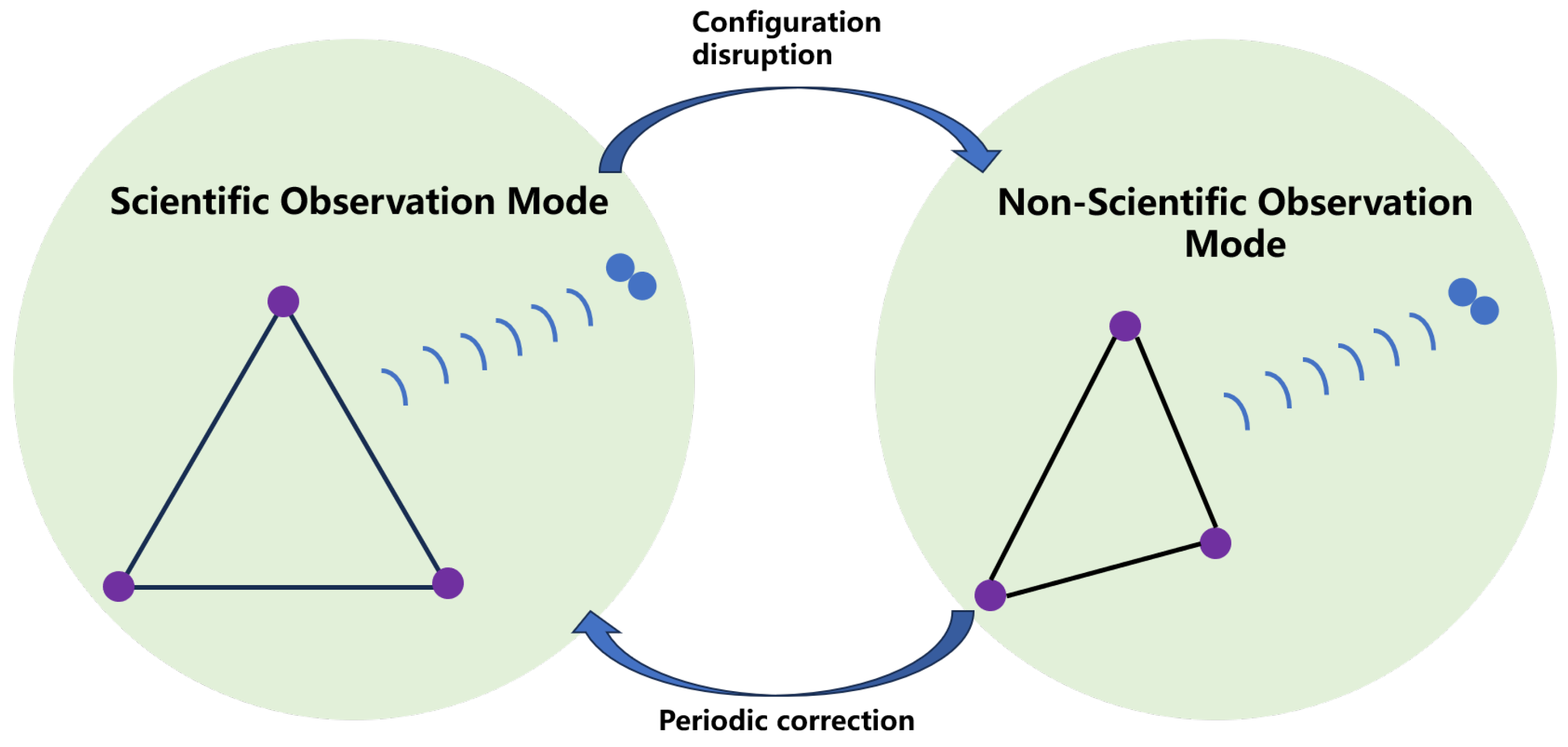
Due to the specific requirements of GWO formation, many researchers have focused solely on near-Earth orbits (“TianQin”), Earth–Sun orbits (“LISA”, “Taiji”, etc.), or Lagrange points $L_3$–$L_5$ (“ASTROD”), because a natural stable equilateral triangle formation can be established, which significantly limits the flexibility of GWOs. To overcome this limitation, two observation modes are proposed in this paper—the scientific observation mode and the non-scientific observation mode, shown in Figure 1. In the scientific observation mode, the spacecraft formation maintains a stable triangle configuration, allowing the laser interferometer to precisely measure the relative positions between the spacecraft, enabling the effective observation of GWs. The shape and relative positions of spacecraft formation remain stable, allowing for high-precision measurements of GWs. To maintain this configuration, periodic small-scale orbital adjustments may be needed to counteract disturbances and instability. Regarding the more scientific observation mode, this paper will not go into detail. However, due to the gravitational forces of various celestial bodies, the formation configuration may be disrupted. Therefore, the non-scientific observation mode is introduced, the spacecraft cannot maintain a constant triangle formation. Hence, control forces are applied to adjust the positions of the spacecraft and maintain the effective formation shape. In this mode, the geometric shape of the formation may not always be an equilateral triangle, and precise control ensures that the spacecraft remain in the correct relative orbits, allowing for continuous observation. Although an optimal GWO may not be possible in this mode, the mission can still operate effectively.

In this paper, a new GWO formation configuration near the Sun–Earth Lagrange point $L_1$ is considered in the non-scientific observation mode, based on output regulation theory. An equilateral triangle array formation and equilateral tetrahedral array formation are proposed. The primary objective of this paper is to propose a control strategy for GWO array formation, which can be applied to the Lagrange point. For the equilateral triangle array formation, two design methods are proposed, and the fuel consumption $\Delta V$ (the $L_1$-norm of the control input) is calculated. For the equilateral tetrahedral array formation, the trajectory and structure of the formation in space are shown.

2. Output Regulation Theory

In this section, the linear output regulation problem is mentioned. The main objective of solving an output regulation problem is to develop a feedback controller that guarantees both asymptotic tracking and effective disturbance rejection while also maintaining the stability of the closed-loop system. Consider a general system defined as follows:

$$\begin{array}{c}\dot{\tilde{\mathit{x}}}=\mathit{A}\tilde{\mathit{x}}+{\mathit{B}}_1\mathit{w}+{\mathit{B}}_2\mathit{u}\hfill \\ \tilde{\mathit{z}}={\mathit{C}}_1\tilde{\mathit{x}}+{\mathit{D}}_{11}\mathit{w}+{\mathit{D}}_{12}\mathit{u}\hfill \\ \tilde{\mathit{y}}={\mathit{C}}_2\tilde{\mathit{x}}+{\mathit{D}}_{21}\mathit{w}\hfill \end{array}$$

(1)

where $\tilde{\mathit{x}}\in {\mathbb{R}}^{\mathrm{n}}$ is the state and the initial value, $\tilde{\mathit{x}}\left(0\right)$ is deterministic, and all the matrices are T-periodic; $\mathit{u}\in {\mathbb{R}}^m$ represents the control input; $\tilde{\mathit{z}}\in {\mathbb{R}}^q$ is the output to be regulated; and $\tilde{\mathit{y}}\in {\mathbb{R}}^p$ is an observation available to the controller. $\mathit{w}\in {\mathbb{R}}^s$ is the signal representing disturbance, and the reference input is modeled by a periodic anti-stable exosystem as follows:

$$\begin{array}{c}\dot{\mathit{w}}=\mathit{Sw}\hfill \\ \mathit{w}\left(0\right)={\mathit{w}}_0\hfill \end{array}$$

(2)

where the initial condition ${\mathit{w}}_0$ is assumed to be deterministic. The output regulation problem involves discovering a stabilizing periodic output feedback controller that drives $\tilde{\mathit{z}}\left(t\right)$ towards zero, despite the influence of the initial conditions $\tilde{\mathit{x}}\left(0\right)$ and ${\mathit{w}}_0$ on the state of the system. To obtain the solvability condition for the output regulation problem, the following assumptions on the system and theorem are established.

Assumption 1.

For periodic systems, the monodromy matrix is stable, and all its eigenvalues (Floquet multipliers) lie within the unit circle in the complex plane.

Assumption 2.

The exosystem is neutrally stable, that is, all the eigenvalues of $\mathit{S}$ are simple and on the imaginary axis and have the same algebraic and geometric multiplicity.

Assumption 3.

$\left[\begin{array}{cc}\left(\begin{array}{cc}{\mathit{C}}_2& {\mathit{D}}_{21}\end{array}\right)& \left(\begin{array}{cc}\mathit{A}& {\mathit{B}}_1\\ 0& \mathit{S}\end{array}\right)\end{array}\right]$ is observable.

Theorem 1.

Suppose that Assumption 1 to Assumption 3 hold. Specifically, the solvability of the control problem and the design of controllers that achieve output tracking can be characterized by the output regulator equations [34]. Moreover, the output regulation problem defined by Equation (1) is solvable, if there exist matrices Π and Γ, which solve Equation (3), often called the regulator equation.

$$\begin{array}{c}\mathit{A}\mathbf{\Pi }-\mathbf{\Pi }\mathit{S}+{\mathit{B}}_1+{\mathit{B}}_2\mathbf{\Gamma }=0\hfill \\ {\mathit{C}}_1\mathbf{\Pi }+{\mathit{D}}_{11}+{\mathit{D}}_{12}\mathbf{\Gamma }=0\hfill \end{array}$$

(3)

where $\left(\mathbf{\Pi },\mathbf{\Gamma }\right)$ denotes the solution of Equation (3). The computation of the regulator in Equation (3) necessitates the use of the matrix $\mathit{S}$.

Proof. 

Given the periodic system (1), where all matrices are T-periodic, an augmented system will be introduced that incorporates periodicity into the state space. Define the augmented state vector as

$$\mathit{\xi }={\left[{\tilde{\mathit{x}}}^T,{\mathit{w}}^T\right]}^T$$

where $\mathit{w}$ is the state of the exosystem. The system dynamics can then be rewritten as

$$\begin{array}{c}\stackrel{.}{\mathit{\xi }}=\left[\begin{array}{cc}\mathit{A}& {\mathit{B}}_1\\ 0& \mathit{S}\end{array}\right]\mathit{\xi }+\left[\begin{array}{c}{\mathit{B}}_2\\ 0\end{array}\right]\mathit{u}\hfill \\ \tilde{\mathit{z}}=\left[\begin{array}{cc}{\mathit{C}}_1& {\mathit{D}}_{11}\end{array}\right]\mathit{\xi }+{\mathit{D}}_{12}\mathit{u}\hfill \end{array}$$

The periodic system is reformulated within an extended linear framework characterized by T-periodic matrices, derived from the dynamics of the exosystem. This transformation facilitates the application of regulator equations to effectively solve the output regulation problem.

The goal of output regulation is to design a control input $\mathit{u}$ such that $\tilde{\mathit{z}}\left(t\right)\to 0$ as $t\to \infty$, regardless of the initial disturbances. This requires solving the output regulator equation (Equation (3)).

Here, $\mathbf{\Pi }$ maps the disturbance state $\mathit{w}$ to the plant state $\tilde{\mathit{x}}$, and $\mathbf{\Gamma }$ determines the control law required to reject disturbances or track references. If the augmented system satisfies Assumptions 1–3, it is controllable and observable, and the output regulator equations have a solution. Therefore, Assumptions 1–3 guarantee the existence of solutions $(\mathbf{\Pi },\mathbf{\Gamma })$ to the regulator equations.

Then, Floquet theory is utilized to analyze the monodromy matrix of the periodic system. When the control input is implemented as a periodic feedback law,

$$\mathit{u}\left(t\right)=\mathit{K}\left(t\right)\tilde{\mathit{y}}\left(t\right)$$

where $\mathit{K}\left(t\right)$ is a periodic matrix. In the closed-loop system, the dynamics of the augmented states are expressed:

$$\dot{\mathit{\xi }}=\left[\begin{array}{cc}\mathit{A}+{\mathit{B}}_2\mathit{K}\left(t\right)& {\mathit{B}}_1\\ 0& \mathit{S}\end{array}\right]\mathit{\xi }$$

Floquet theory states that the stability of this periodic system is determined by the monodromy matrix, the state transition matrix over one period T. If all Floquet multipliers (eigenvalues of the monodromy matrix) lie within the unit circle in the complex plane, the system is stable. By appropriately designing $\mathit{K}\left(t\right)$, closed-loop system stability is ensured.

Based on Assumption 2, $\mathit{S}$ is neutrally stable, with its eigenvalues residing on the imaginary axis and possessing equal algebraic and geometric multiplicities. Under these conditions, the solution $(\mathbf{\Pi },\mathbf{\Gamma })$ can be utilized to design a control law that ensures $\tilde{\mathit{z}}\left(t\right)\to 0$, enabling the system to achieve both disturbance rejection and reference tracking. □

3. The GWO Array Formation Configuration Design

In this section, the design of the GWO array formation configuration will be introduced in detail, including a comprehensive overview of both the equilateral triangle array formation and equilateral tetrahedral array formation.

3.1. Dynamic Equation

A. Circular restricted three-body problem

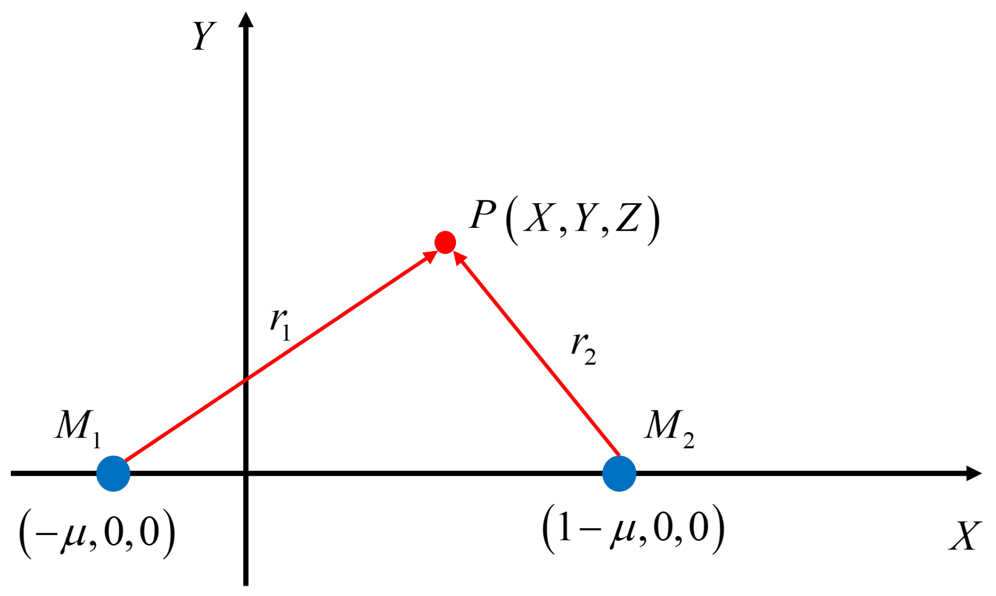
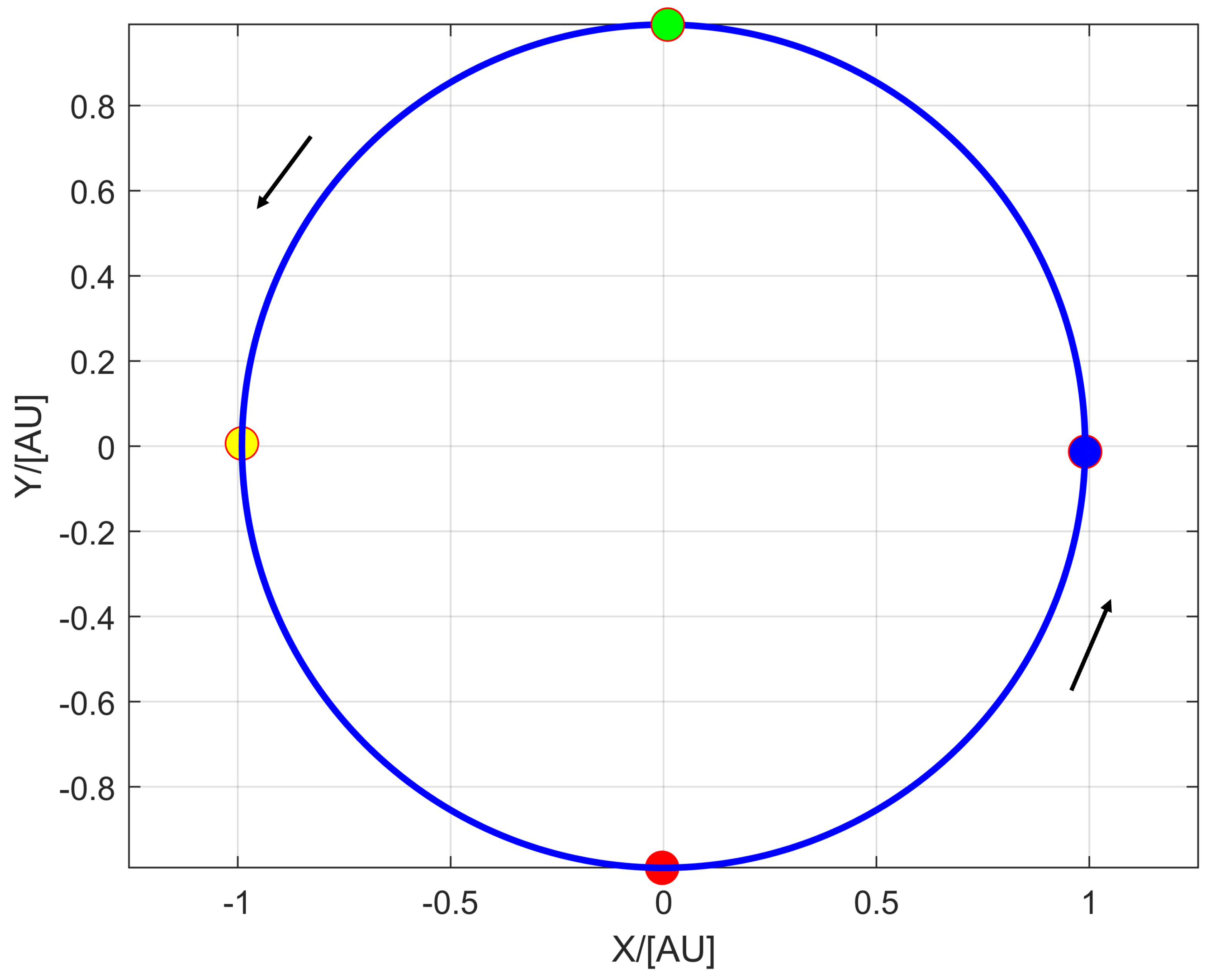
The circular restricted three-body problem (CRTBP) elucidates the orbital dynamics of a spacecraft, denoted as P, influenced by the gravitational forces exerted by two massive celestial bodies, $M_1$ and $M_2$, where $M_1$ and $M_2$ are the masses of the Sun and Earth, respectively, as shown in Figure 2. Suppose that $\left(X,Y,Z\right)$, $\left(-\mu ,0,0\right)$, and $\left(1-\mu ,0,0\right)$ describe the non-dimensional coordinates of the spacecraft, Sun and Earth, respectively. The equations of motion in non-dimensional form are expressed as follows:

$$\begin{array}{c}{\displaystyle \ddot{X}-2\dot{Y}-X=-\frac{1-\mu }{r_1^3}\left(X+\mu \right)-\frac{\mu }{r_2^3}\left(X+\mu -1\right)+u_x}\hfill \\ {\displaystyle \ddot{Y}+2\dot{X}-Y=-\frac{1-\mu }{r_1^3}Y-\frac{\mu }{r_2^3}Y+u_y}\hfill \\ {\displaystyle \ddot{Z}=-\frac{1-\mu }{r_1^3}Z-\frac{\mu }{r_2^3}Z+u_z}\hfill \end{array}$$

(4)

where $\{X,Y,Z\}$ represents the rotating frame with its origin at the barycenter of the system, $\left\{u_x,u_y,u_z\right\}$ is the control acceleration, $\mu =M_2/\phantom{M_2\left(M_1+M_2\right)}\left(M_1+M_2\right)$, $M_1>M_2$, and the distances between spacecraft $M_1$ and $M_2$ are, respectively, given by $r_1$ and $r_2$ as follows:

$$\begin{array}{c}{r}_1=\sqrt{{\left(X+\mu \right)}^2+Y^2+Z^2}\hfill \\ r_2=\sqrt{{\left(X+\mu -1\right)}^2+Y^2+Z^2}\hfill \end{array}$$

Equation (4) has libration points known as Lagrange points because the equations of motion are normalized.

$$\begin{array}{ccc}{\displaystyle X=\frac{1-\mu }{r_1^3}\left(X+\mu \right)+\frac{\mu }{r_2^3}\left(X+\mu -1\right)}& {\displaystyle Y=\frac{1-\mu }{r_1^3}Y+\frac{\mu }{r_2^3}Y}& Z=0\end{array}$$

(5)

And the Lagrange points $L_i$$\left(i=1,2,3,4,5\right)$ are expressed as follows,

$$\begin{array}{c}\begin{array}{ccc}{L}_1=\left(l_1\left(\mu \right),0,0\right)& L_2=\left(l_2\left(\mu \right),0,0\right)& L_3=\left(l_3\left(\mu \right),0,0\right)\end{array}\hfill \\ \begin{array}{cc}{L}_4=\left(1/\phantom{12-\mu }2-\mu ,\sqrt{3}/\phantom{\sqrt{3}2}2,0\right)& L_5=\left(1/\phantom{12-\mu }2-\mu ,-\sqrt{3}/\phantom{-\sqrt{3}2}2,0\right)\end{array}\hfill \end{array}$$

where the values of $l_i$ are determined by Equation (5). To describe the equations of motion near a collinear equilibrium point $L_i\left(i=1,2,3\right)$, it is convenient to use the coordinate system with its center located at $L_i$. Replacing $X,Y,Z$ with $x+l_i,y,z$, the equations of motion in the non-dimensional form are given by [32]

$$\begin{array}{c}{\displaystyle \ddot{x}-2\dot{y}-x=l_i-\frac{1-\mu }{r_1^3}\left(x+l_i+\mu \right)-\frac{\mu }{r_2^3}\left(x+l_i-1+\mu \right)+u_x}\hfill \\ {\displaystyle \ddot{y}+2\dot{x}-y=-\frac{1-\mu }{r_1^3}y-\frac{\mu }{r_2^3}y+u_y}\hfill \\ {\displaystyle \ddot{z}=-\frac{1-\mu }{r_1^3}z-\frac{\mu }{r_2^3}z+u_z}\hfill \end{array}$$

(6)

where $r_1=\sqrt{{\left(x+l_i+\mu \right)}^2+y^2+z^2}$, $r_2=\sqrt{{\left(x+l_i-1+\mu \right)}^2+y^2+z^2}$

The linearized equations of motion about the collinear equilibrium points can be given as

$$\begin{array}{c}\ddot{x}-2\dot{y}-\left(2{\sigma }_i+1\right)x=u_x\hfill \\ \ddot{y}+2\dot{x}+\left({\sigma }_i-1\right)y=u_y\hfill \\ \ddot{z}+{\sigma }_{i}z=u_z\hfill \end{array}$$

(7)

where ${\displaystyle {\sigma }_i=\frac{\mu }{{\left|l_i+\mu -1\right|}^3}+\frac{1-\mu }{{\left|l_i+\mu \right|}^3}}$

Next, Equation (7) can be rewritten in the state space form as

$$\dot{\mathit{x}}=\mathit{Ax}+\mathit{Bu}$$

(8)

where $\mathit{x}=\left[\begin{array}{c}x\\ y\\ \dot{x}\\ \dot{y}\\ z\\ \dot{z}\end{array}\right],\mathit{u}=\left[\begin{array}{c}{u}_x\\ u_y\\ u_z\end{array}\right],$

$\mathit{A}=\left[\begin{array}{cccccc}0& 0& 1& 0& 0& 0\\ 0& 0& 0& 1& 0& 0\\ 2{\sigma }_i+1& 0& 0& 2& 0& 0\\ 0& 1-{\sigma }_i& -2& 0& 0& 0\\ 0& 0& 0& 0& 0& 1\\ 0& 0& 0& 0& -{\sigma }_i& 0\end{array}\right],\mathit{B}=\left[\begin{array}{ccc}0& 0& 0\\ 0& 0& 0\\ 1& 0& 0\\ 0& 1& 0\\ 0& 0& 0\\ 0& 0& 1\end{array}\right]$

Likewise, the state space form of Equation (6) is semi-linear, and it is expressed as

$$\dot{\mathit{x}}=\mathit{Ax}+\mathit{B}f\left(\mathit{x}\right)+\mathit{Bu}$$

(9)

where $f\left(x\right)$ represents the nonlinear components, and is written as

$$f\left(\mathit{x}\right)=\left[\begin{array}{c}{\displaystyle l_i-2{\sigma }_{i}x-\frac{1-\rho }{r_1^3}\left(x+l_i+\rho \right)-\frac{\rho }{r_2^3}\left(x+l_i-1+\rho \right)}\\ {\displaystyle {\sigma }_{i}y-\frac{1-\rho }{r_1^3}y-\frac{\rho }{r_2^3}y}\\ {\displaystyle {\sigma }_{i}z-\frac{1-\rho }{r_1^3}z-\frac{\rho }{r_2^3}z}\end{array}\right]$$

B. Ephemeris model

The CRTBP serves as an essential and effective framework for analyzing trajectories within multi-body dynamical systems, capturing and modeling a wide range of behaviors. However, when dealing with complex scenarios, particularly those involving intricate gravitational interactions or the influence of additional celestial bodies, the CRTBP may fall short. In such cases, a more sophisticated model is necessary that can incorporate higher-fidelity considerations, including perturbations from celestial bodies not accounted for in the standard CRTBP. This enhanced modeling approach allows for more accurate predictions in complex environments.

The ephemeris model distinguishes itself as a higher-fidelity approach to celestial dynamics. In this model, the gravitational influence of multiple celestial bodies (typically denoted as N bodies) affects the motion of each individual celestial body within the system. It provides a more detailed and accurate representation of the complex interactions between celestial bodies. These celestial bodies typically include planets, moons, and other significant objects, along with the spacecraft of interest. By incorporating the gravitational influences of these additional celestial bodies, the ephemeris model allows for more accurate trajectory predictions.

For the design of GWO formation orbits, the Jet Propulsion Laboratory Planetary Ephemerides (JLP) is employed. This model is simplified based on the following considerations:

1. Only three celestial bodies are taken into account—the Sun, Moon, and Earth.

2. To establish the equations of motion for the ephemeris model, the differential equations are expressed within the inertial frame [35], as shown in Figure 3a.

$$m\ddot{\mathit{r}}=-G\sum _{i=1}^N{\displaystyle \frac{m{M}_i}{r_i^3}}{\mathit{r}}_i$$

(10)

where ${\mathit{M}}_i$ is the location of the celestial body of interest.

3. The relative formulation of the celestial body equations of motion, describing the movement of the target celestial body with respect to the central celestial body and accounting for the influence of both the central and other perturbing celestial bodies (as shown in Figure 3b), is given as follows:

$$m\ddot{\mathit{r}}=-G{\displaystyle \frac{m{M}_0}{r_0^3}}{\mathit{r}}_0-G\sum _{i=1}^{N}n{M}_i\left({\displaystyle \frac{{\mathit{r}}_i}{r_i^3}}-{\displaystyle \frac{{\mathit{r}}_{0i}}{r_{0i}^3}}\right)$$

(11)

where ${\mathit{M}}_0$ represents evolution under the influence of other perturbing celestial bodies.

The relative position vector, representing the location of the perturbing celestial bodies relative to the central celestial body, was obtained from NAIF’s SPICE library [36].

3.2. Formation Configuration Design

In this section, the GWO formation configuration design will be introduced. Traditionally, a GWO formation consists of three spacecraft, and its arm-length constrains the frequency range of the GWO. The noise level of the laser interferometer is very high owing to the extremely weak intensity of GWs; therefore, sensitivity is defined as a critical parameter. Here, additional assumptions are given:

Assumption 4.

The change in arm-length caused by GWs is proportional to both the original arm-length and the amplitude and frequency of the GWs.

Assumption 5.

The detector’s sensitivity is directly related to the change in arm-length, which is proportional to the nominal arm-length. There exists an optimal nominal arm-length that maximizes the detector’s sensitivity within a specific target frequency band.

Assumption 6.

The change in the spacetime metric tensor due to GWs is linear; both smaller and larger GW perturbations cause proportionally smaller or larger changes in arm-length, respectively, with these changes being dependent on the GWs’ strength and frequency.

Based on the above assumptions, the arm-length of the interferometer is denoted as L. When GWs arrive, depending on the characteristics of the GWs, one arm elongates while the other arm simultaneously contracts in a perpendicular manner. Representing the change in arm-length as $\Delta L$, the two arm-lengths become $L+\Delta L$ and $L-\Delta L$, respectively. The sensitivity, denoted as $h_d$, is defined as

$$h_d={\displaystyle \frac{\Delta L}{L}}$$

(12)

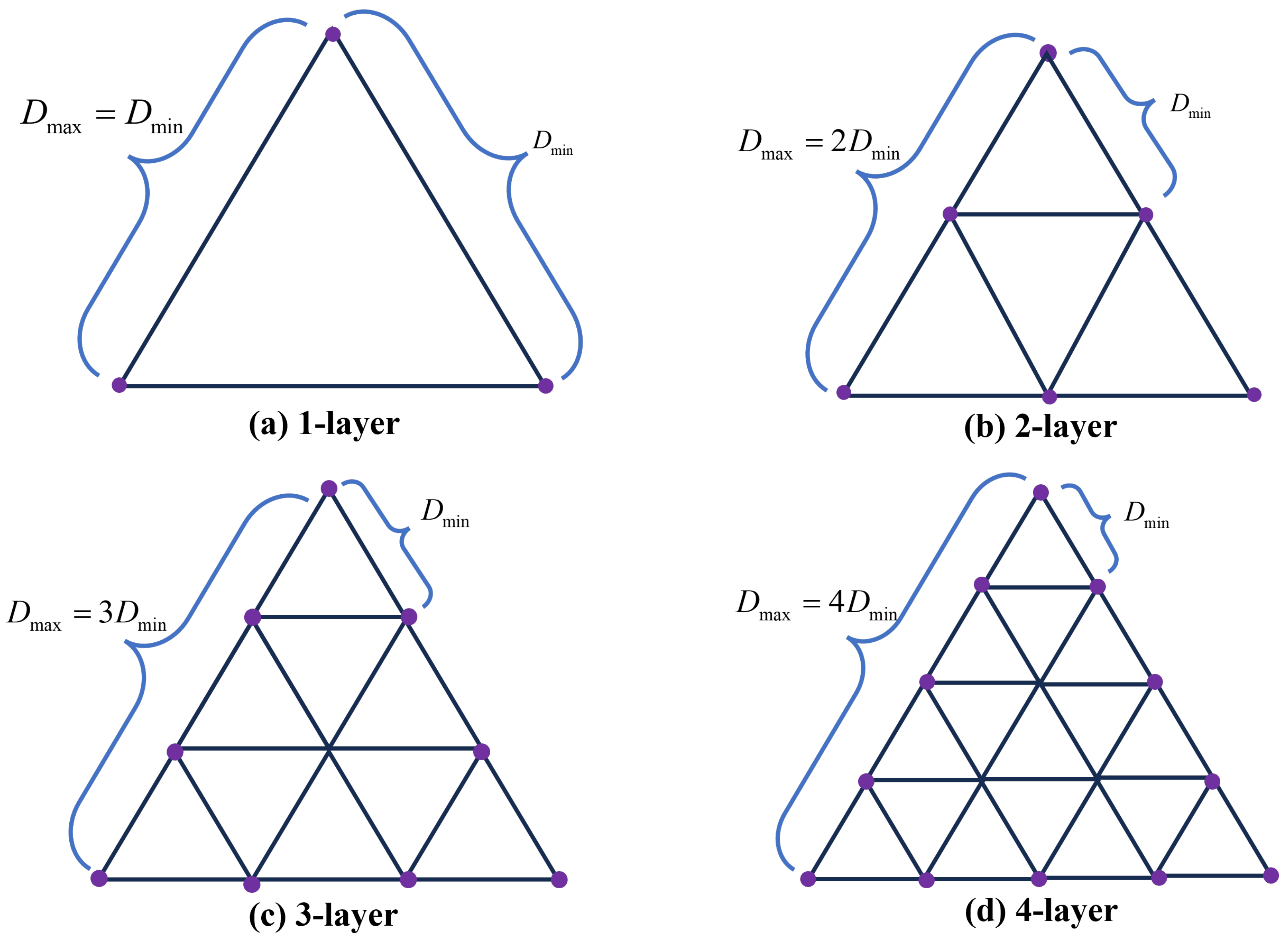
In Equation (12), since $\Delta L$ is much smaller than L, the sensitivity decreases as the arm-length increases. To improve sensitivity and mitigate laser attenuation, array formation is proposed. In this paper, the equilateral triangle array formation and equilateral tetrahedral array formation are introduced, as illustrated in Figure 4 and Figure 5.

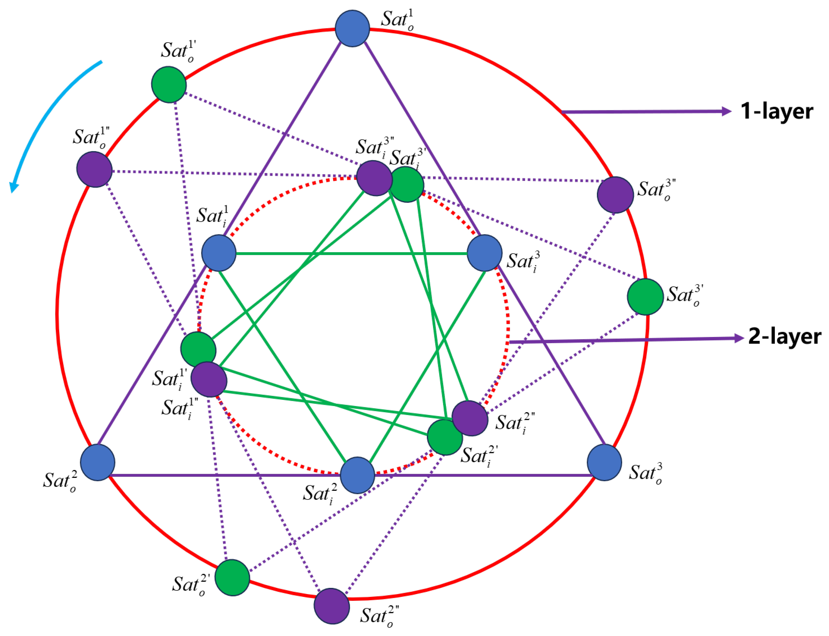
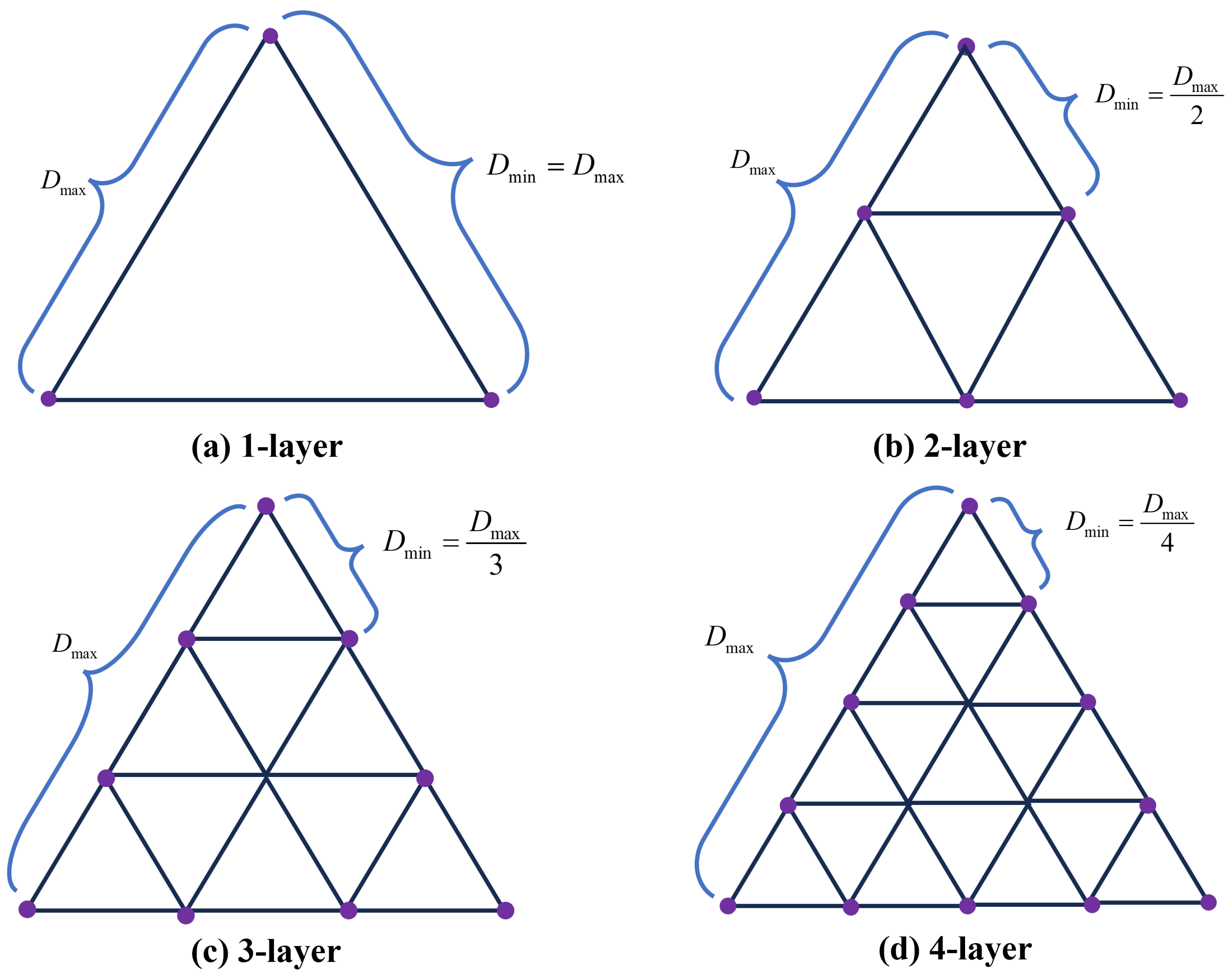
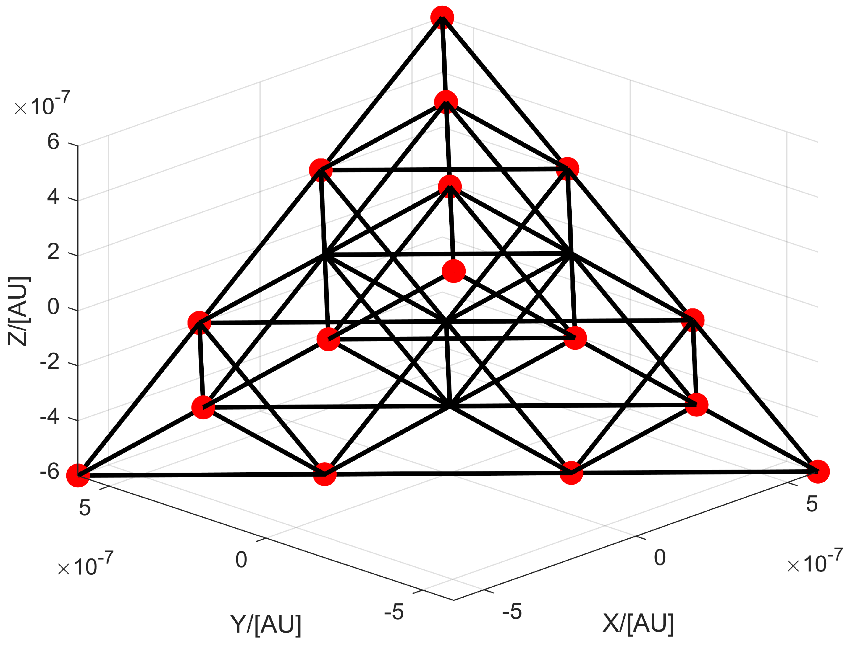
In Figure 4, a multi-layer equilateral triangle array formation is designed (only two-layer is shown in this figure). Multiple spacecraft are deployed on each side, forming a “nested” configuration. This method effectively mitigates laser attenuation and allows for longer baselines. The spacecraft at the vertices are the chief spacecraft, while the other spacecraft serve as deputy spacecraft. Acting as a “bridge” between the chief spacecraft, the deputy spacecraft can effectively amplify the laser optical path. 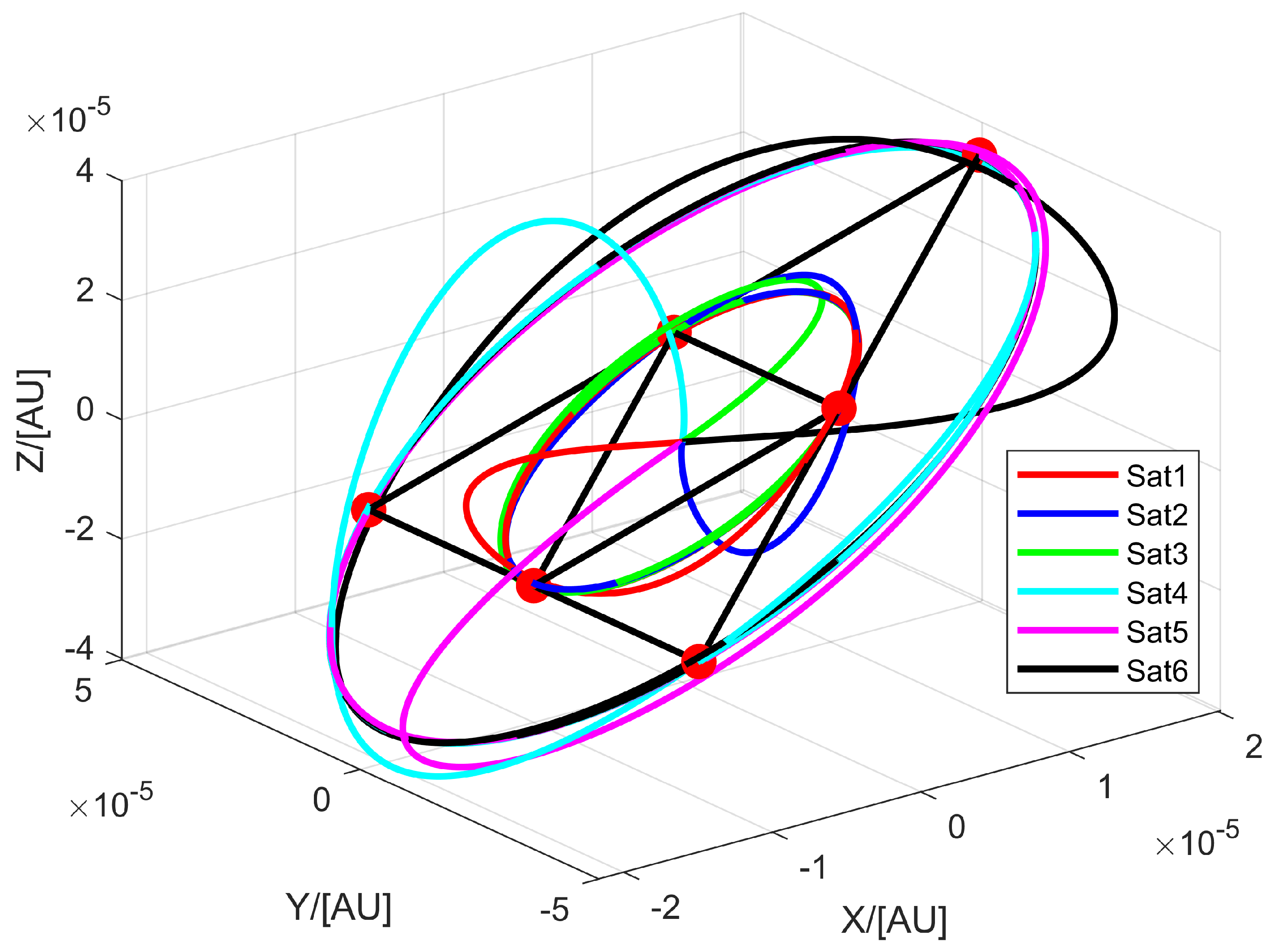In Figure 5, an equilateral tetrahedral array formation is designed, which can effectively observe GWs and avoid configuration/reconfiguration issues when observing GWs in different directions. In addition, this method can enable fixed-point observation of GWs. Redesigning of the optical path is required, in order to change the optical path by adjusting the attitude of the test masses (TMs). Regarding the design of the optical path, this paper will not go into detail.

Next, the two methods will be expressed based on the output regulation theory.

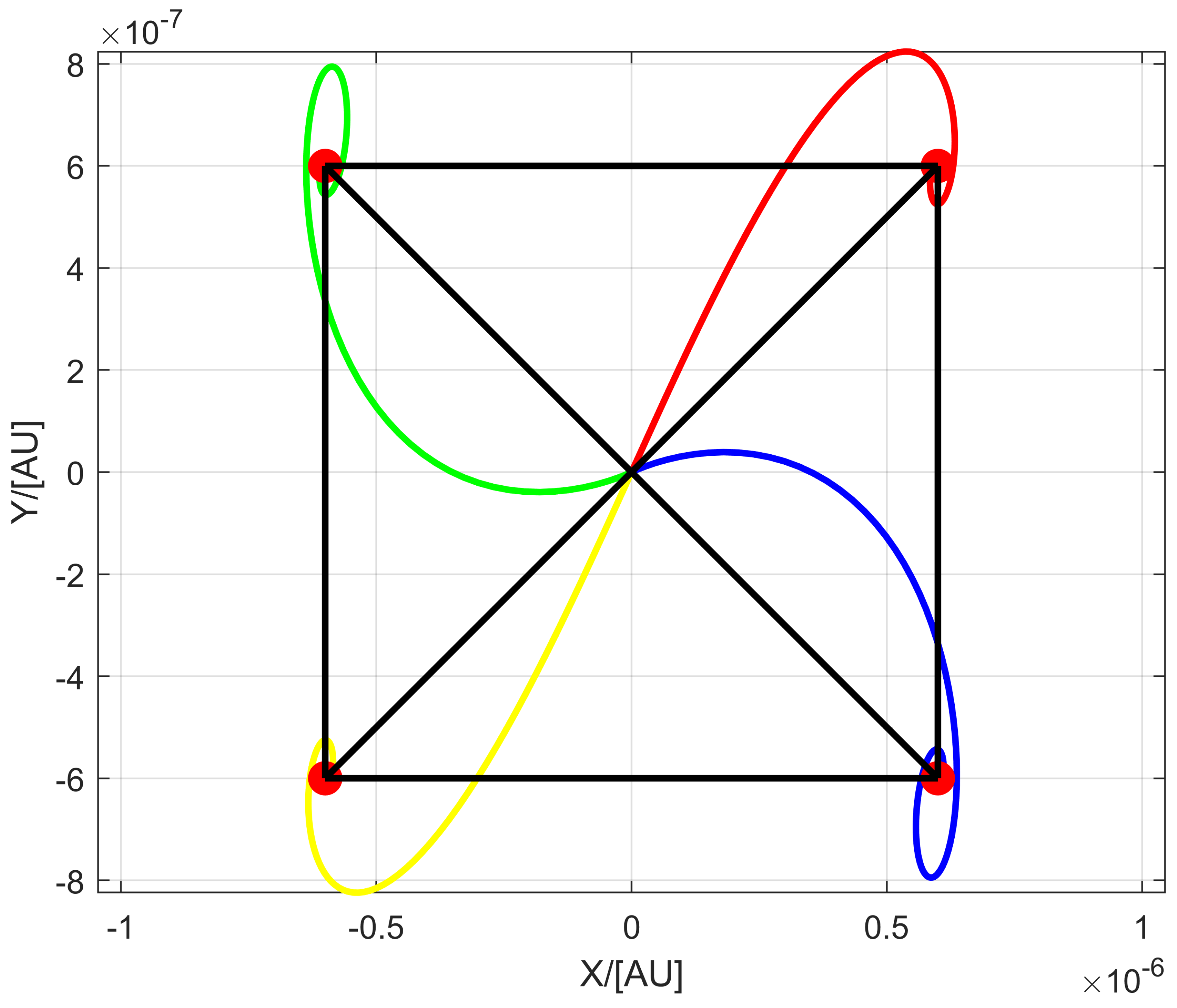
3.2.1. The Equilateral Triangle Array Formation

This part derives the control law to establish and maintain the triangle formation using the output regulation theory. The reference orbit of the deputy spacecraft follows a periodic trajectory modeled through a sinusoidal function, enabling it to complete the equilateral triangle array formation within a given period. Specifically, the triangle array formation in which the chief spacecraft is situated near Lagrange point $L_i$, as defined by Equation (13), is considered. The reference orbit of the deputy spacecraft is represented by $\left(x_l+w_1,y_l+w_2,z_l+w_3\right)$. Here, $\left(w_1,w_2,w_3\right)$ represents a periodic relative orbit of the deputy spacecraft.

$$\begin{array}{cc}{\dot{\mathit{x}}}_l=\mathit{A}{\mathit{x}}_l+\mathit{B}f\left({\mathit{x}}_l\right),& {\mathit{x}}_l\left(0\right)={\mathit{x}}_{l0}\end{array}$$

(13)

where $x_l$ represents a periodic orbit of the chief spacecraft near Lagrange point $L_i$. As for the $\left(w_1,w_2,w_3\right)$, it is given by

$$\begin{array}{c}{w}_1\left(t\right)=acos({\omega }_{1}t+{\tau }_i)\hfill \\ w_2\left(t\right)=2asin({\omega }_{1}t+{\tau }_i)\hfill \\ w_3\left(t\right)=\sqrt{3}acos({\omega }_{2}t+{\tau }_i)\hfill \\ \begin{array}{cc}{\displaystyle {\tau }_i=0,\frac{2}{3}\pi ,\frac{4}{3}\pi }& (i=1,2,3)\end{array}\hfill \end{array}$$

(14)

where a is the parameter that determines the orbital radius.

Equation (14) provides a periodic reference orbit. The trajectory (defined by Equation (14)) is generated as follows:

$$\begin{array}{cc}\dot{\mathit{w}}=\mathit{Sw},& \mathit{w}\left(0\right)={\mathit{w}}_0\end{array}$$

(15)

where

$$\mathit{S}=\left[\begin{array}{cccc}0& s_1& 0& 0\\ s_2& 0& 0& 0\\ 0& 0& 0& 1\\ 0& 0& -{\omega }_2^2& 0\end{array}\right],s_1=-{\displaystyle \frac{{\omega }_1}{2}},s_2=2{\omega }_1,{\omega }_2>0$$

To establish the prescribed formation and maintain it, the output regulation theory needs to be modified. Given the general system (described by Equation (1)) and exogenous system (described by Equation (2)), the output regulation problem involves finding a control law such that $\tilde{\mathit{z}}\left(t\right)$ converges to zero as time goes to infinity for any initial conditions of the exosystem. In accordance with Assumption and Equation (3), admissible controllers are expressed as

$$\mathit{u}=-\mathit{Fx}+\left(\mathbf{\Gamma }+\mathit{F}\mathbf{\Pi }\right)\mathit{w}$$

(16)

where $\mathit{F}$ is an arbitrary feedback gain such that $\mathit{A}-\mathit{BF}$ is asymptotically stable. Likewise, the equilateral triangle array formation problem for the semi-linear system can be solved by the nonlinear feedback control given by

$$\mathit{u}=-\mathit{Fe}+f\left({\mathit{x}}_l\right)-f\left(\mathit{x}\right)+\left(\mathbf{\Gamma }+\mathit{F}\mathbf{\Pi }\right)\mathit{w}$$

(17)

where $\mathit{e}=\mathit{x}-{\mathit{x}}_l$.

Proof. 

Substituting the control law (Equation (17)) into System (9),

$$\begin{array}{c}\dot{\mathit{x}}=\mathit{Ax}+\mathit{B}f\left(\mathit{x}\right)+\mathit{B}\left(-\mathit{Fe}+f\left({\mathit{x}}_l\right)-f\left(\mathit{x}\right)+\left(\mathbf{\Gamma }+\mathit{F}\mathbf{\Pi }\right)\mathit{w}\right)\hfill \\ =\mathit{Ax}-\mathit{BFe}+\mathit{B}f\left({\mathit{x}}_l\right)-\mathit{B}f\left(\mathit{x}\right)+\mathit{B}\left(\mathbf{\Gamma }+\mathit{F}\mathbf{\Pi }\right)\mathit{w}\hfill \end{array}$$

Defining the error $\mathit{e}=\mathit{x}-{\mathit{x}}_l$ and differentiating it yields $\dot{\mathit{e}}=\dot{\mathit{x}}-{\dot{\mathit{x}}}_l$.

Substituting the expressions for $\dot{\mathit{x}}$ and ${\dot{\mathit{x}}}_l$,

$$\begin{array}{c}\dot{\mathit{e}}=\left(\mathit{Ax}-\mathit{BFe}+\mathit{B}f\left({\mathit{x}}_l\right)-\mathit{B}f\left(\mathit{x}\right)+\mathit{B}\left(\mathbf{\Gamma }+\mathit{F}\mathbf{\Pi }\right)\mathit{w}\right)-\left(\mathit{A}{\mathit{x}}_l+\mathit{B}f\left({\mathit{x}}_l\right)\right)\hfill \\ =\mathit{Ae}-\mathit{BFe}+\mathit{B}\left(\mathbf{\Gamma }+\mathit{F}\mathbf{\Pi }\right)\mathit{w}\hfill \end{array}$$

The error dynamics can now be written as

$$\dot{\mathit{e}}=\left(\mathit{A}-\mathit{BF}\right)\mathit{e}+\mathit{B}\left(\mathbf{\Gamma }+\mathit{F}\mathbf{\Pi }\right)\mathit{w}$$

From the regulator equation,

$$\mathit{A}\mathbf{\Pi }-\mathbf{\Pi }\mathit{S}+\mathit{B}\mathbf{\Gamma }=0$$

The term $\mathbf{\Gamma }+\mathit{F}\mathbf{\Pi }$ ensures that the regulation error converges to zero, satisfying the output regulation condition. Furthermore, the matrix $\mathit{A}-\mathit{B}\mathit{F}$ is designed to be Hurwitz, guaranteeing the asymptotic stability of the error dynamics.

Thus, the control law in Equation (17) ensures that the error $\mathit{e}\left(t\right)$ converges to zero as $t\to \infty$, achieving the desired trajectory tracking.

If the full state is available ($y=x$), then the regulator equation given by Equation (3) is reduced to

$$\begin{array}{c}\mathit{A}\mathbf{\Pi }-\mathbf{\Pi }\mathit{S}+\mathit{B}\mathbf{\Gamma }=0\hfill \\ \mathit{C}\mathbf{\Pi }+{\mathit{D}}_1=0\hfill \end{array}$$

(18)

where

$$\mathit{C}=\left[\begin{array}{cccccc}1& 0& 0& 0& 0& 0\\ 0& 1& 0& 0& 0& 0\\ 0& 0& 0& 0& 1& 0\end{array}\right],{\mathit{D}}_1=-\left[\begin{array}{cccc}1& 0& 0& 0\\ 0& 1& 0& 0\\ 0& 0& 1& 0\end{array}\right]$$

By solving Equation (18), $\mathbf{\Pi }$ and $\mathbf{\Gamma }$ can be sought as

$$\begin{array}{c}\mathbf{\Pi }={\left[\begin{array}{cccccc}1& 0& 0& s_2& 0& 0\\ 0& 1& s_1& 0& 0& 0\\ 0& 0& 0& 0& 1& 0\\ 0& 0& 0& 0& 0& 1\end{array}\right]}^T\hfill \\ \mathbf{\Gamma }={\left[\begin{array}{ccc}{s}_1{s}_2-2s_2-2{\sigma }_i-1& 0& 0\\ 0& s_1{s}_2+2s_1-1+{\sigma }_i& 0\\ 0& 0& -{\omega }_2^2+{\sigma }_i\\ 0& 0& 0\end{array}\right]}^T\hfill \end{array}$$

where ${\displaystyle s_1=-\frac{{\omega }_1}{2},s_2=2{\omega }_1,{\omega }_2>0}$. □

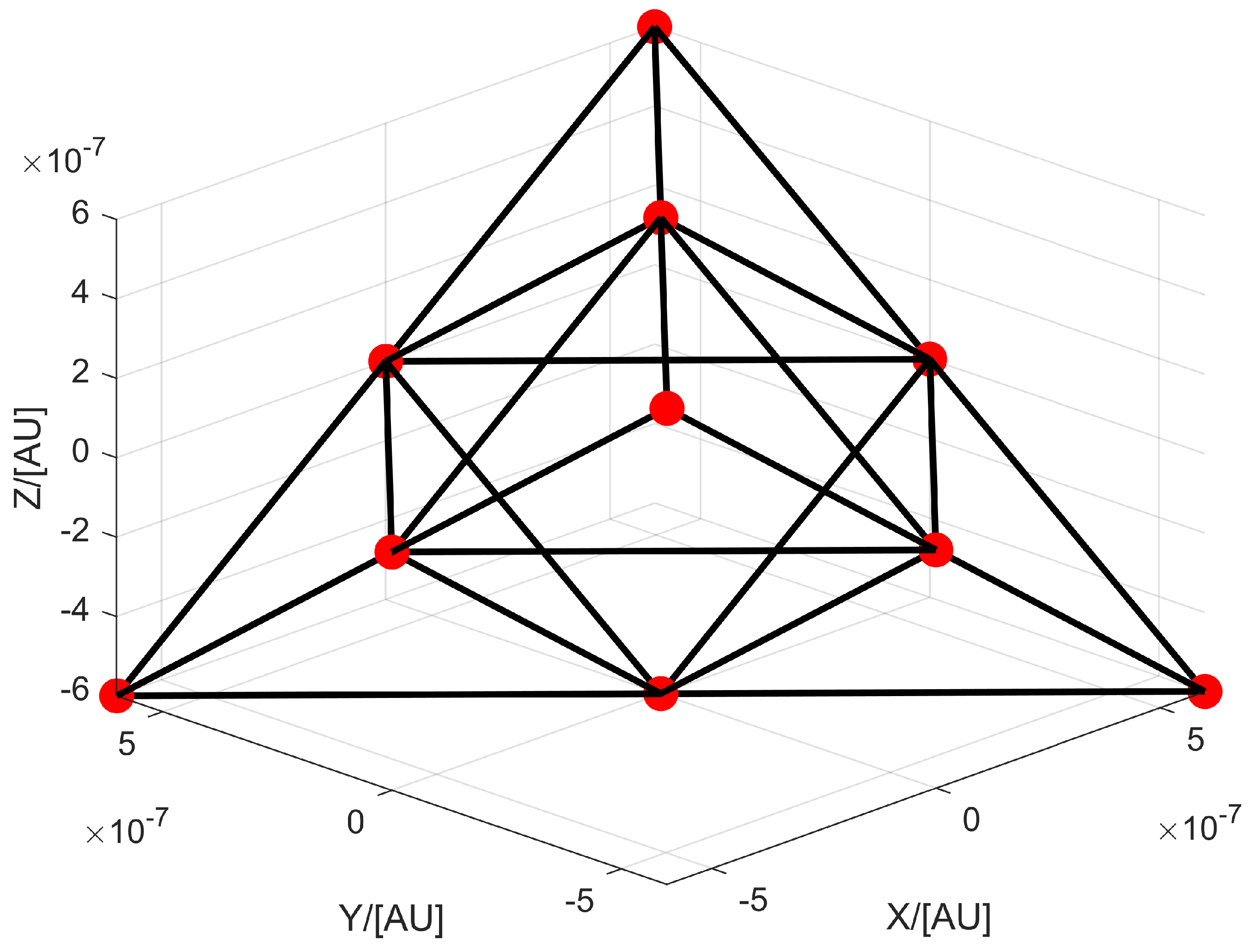
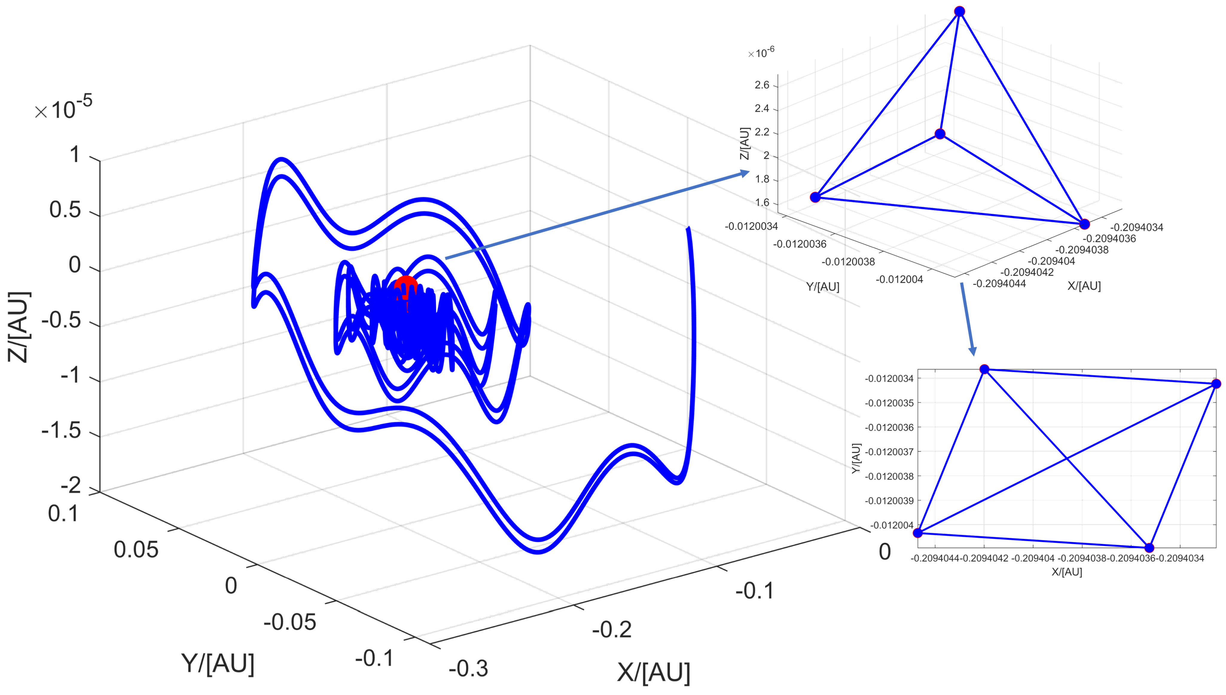
3.2.2. The Equilateral Tetrahedral Array Formation

For the equilateral tetrahedral array formation, the design method is similar to the equilateral triangle array formation, and $\mathit{w}$ is given to implement fixed-point formation.

$$\begin{array}{c}{w}_{1,tetra}=\left[0.0006a,0.0006a,0.0006a\right]\hfill \\ w_{2,tetra}=\left[0.0006a,-0.0006a,-0.0006a\right]\hfill \\ w_{3,tetra}=\left[-0.0006a,0.0006a,-0.0006a\right]\hfill \\ w_{4,tetra}=\left[-0.0006a,-0.0006a,0.0006a\right]\hfill \end{array}$$

(19)

$${\mathit{S}}_{tetra}=\left[\begin{array}{ccc}0& 0& 0\\ 0& 0& 0\\ 0& 0& 0\end{array}\right]$$

The solution to the regulator equation is explicitly given by

$$\begin{array}{c}{\mathbf{\Pi }}_{tetra}=\left[\begin{array}{ccc}1& 0& 0\\ 0& 1& 0\\ 0& 0& 0\\ 0& 0& 0\\ 0& 0& 1\\ 0& 0& 0\end{array}\right],{\mathbf{\Gamma }}_{tetra}=\left[\begin{array}{ccc}-2{\sigma }_i-1& 0& 0\\ 0& {\sigma }_i-1& 0\\ 0& 0& {\sigma }_i\end{array}\right]\hfill \\ {\mathit{C}}_{tetra}=\left[\begin{array}{cccccc}1& 0& 0& 0& 0& 0\\ 0& 1& 0& 0& 0& 0\\ 0& 0& 0& 0& 1& 0\end{array}\right],{\mathit{D}}_{1,tetra}=-\left[\begin{array}{ccc}1& 0& 0\\ 0& 1& 0\\ 0& 0& 1\end{array}\right]\hfill \end{array}$$

4. Simulation Result

In this section, output regulation theory is applied to establish and maintain the equilateral triangle array formation and equilateral tetrahedral array formation. Simultaneously, the design parameters are examined in terms of the total cost. The control laws described by Equations (16) and (17) are applied to the equations of motion for the Sun–Earth CRTBP. The Lagrange point is specified as $L_1$. The period and radius of the Sun–Earth system are $T_0=365.26$ days and $R_0=1.4960\times {10}^8$ [km] ( = 1 [AU]), respectively. The remaining parameters are $\rho =3.0542\times {10}^{-6}$, ${\sigma }_1=4.0611$, and $a=1\times {10}^{-6}$ [AU] ($\approx 1.49\times {10}^2$ km), with the phase angles of the equilateral triangle array formation specified at $\left[{\tau }_1,{\tau }_2,{\tau }_3\right]=\left[0^{\circ },{120}^{\circ },{240}^{\circ }\right]$. To maintain the reference orbit, feedback control is essential. The feedback gain $\mathit{F}$ for the feedback term in Equations (16) and (17) can be chosen arbitrarily, provided that $\mathit{A}-\mathit{BF}$ is asymptotically stable. In this paper, the feedback gain is designed based on linear quadratic regulator theory, in which the gain is defined as $\mathit{F}={\mathit{R}}^{-1}\dot{\mathit{B}}\mathit{X}$, with $\mathit{X}$ being the solution of the Riccati Equation (20), $\mathit{Q}=\mathit{I}$, and $\mathit{R}=\mathit{I}$. The $\Delta V$ required to maintain this orbit in two periods is evaluated.

$${\mathit{A}}^T\mathit{X}+\mathit{XA}+\mathit{Q}-\mathit{XB}{\mathit{R}}^{-1}{\mathit{B}}^T\mathit{X}=0$$

(20)

4.1. Equilateral Triangle Array Formation in CRTBP

In this subsection, the array spacecraft’s initial state ${\tilde{\mathit{x}}}_i\left(0\right),(i=1,2,3,\dots )$ is given by

$${\tilde{\mathit{x}}}_i\left(0\right)=\left[0,0,0,0,0,0\right]$$

(21)

and the initial conditions ${\mathit{w}}_i\left(0\right),(i=1,2,3,\dots )$ are

$$\begin{array}{c}{\mathit{w}}_i\left(0\right)=[acos{\tau }_i,2asin{\tau }_i,\sqrt{3}acos{\tau }_i,-\sqrt{3}a{\omega }_{1}sin{\tau }_i]\hfill \\ \begin{array}{cc}{\displaystyle {\tau }_i=0,\frac{2}{3}\pi ,\frac{4}{3}\pi }& (i=1,2,3)\end{array}\hfill \end{array}$$

A two-layer equilateral triangle array formation, covering six spacecraft, is shown in Figure 6. The equilateral triangle array formation is established in two periods owing to the output regulation. The equilateral triangle array formation includes an out-circle formation and an in-circle formation. The out-circle formation comprises three spacecraft at the vertices, while the remaining spacecraft establish an in-circle formation.

The error histories of the spacecraft are shown in Figure 7. As seen in Figure 7, the errors converge to zero, indicating that the spacecraft have completed the initialization process and are maintained by the control law. The maximum errors, determined by the absolute value of the difference between the linear system and nonlinear system, are $\left[1.34,5.10,1.36\right]\times {10}^{-7}$ [AU] for Sat1 (in-circle), $\left[0.042,0.43,3.58\right]\times {10}^{-7}$ [AU] for Sat2 (in-circle), $\left[0.99,2.48,3.08\right]\times {10}^{-7}$ [AU] for Sat3 (in-circle), $\left[2.24,0.44,7.26\right]\times {10}^{-7}$ [AU] for Sat1 (out-circle), $\left[2.02,10.61,5.23\right]\times {10}^{-7}$ [AU] for Sat2 (out-circle), and $\left[1.16,5.08,3.61\right]\times {10}^{-7}$ [AU] for Sat3 (out-circle).

To prove that an equilateral triangle array formation is achieved, let us define

$$\begin{array}{c}{d}_i\left(t\right)=\sqrt{w_{ix}^2\left(t\right)+w_{iy}^2\left(t\right)+w_{iz}^2\left(t\right)}\hfill \\ \left(i=1,2,3,4,5,6\right)\hfill \end{array}$$

(22)

As time passes, $d_i$ approaches a constant values (see Figure 8), indicating that an equilateral triangle array formation has been established.

To more intuitively illustrate the array nature of the formation, the three-layer equilateral triangle array formation is shown in Figure 9. The yellow point represents a virtual spacecraft, and there are two spacecraft distributed between each of the two vertices; the three-layer equilateral triangle array formation is established.

Then, the stability of the formation after initialization is analyzed. After the formation initialization is completed, additional control forces are required to maintain the stability of formation configuration. Taking one-layer equilateral triangle formation as an example, the control forces are shown in Figure 10. The maximum control forces required to maintain the formation are approximately $\left[8.413,5.969,3.189\right]\times {10}^{-7}\left[\mathrm{m}/{\mathrm{s}}^2\right]$ (for Sat1), $\left[8.389,1.288,3.321\right]\times {10}^{-7}\left[\mathrm{m}/{\mathrm{s}}^2\right]$ (for Sat2), and $\left[8.403,1.341,3.146\right]\times {10}^{-7}\left[\mathrm{m}/{\mathrm{s}}^2\right]$ (for Sat3).

Next, the total $\Delta V$ ($L_1$-norm of all spacecraft control inputs) and average $\Delta V$ (the total $\Delta V$/number of spacecraft) required for the transition to the final orbit and to maintain it for two periods are calculated. Two cases are calculated.

4.1.1. Case 1. Fixed Outer-Edge Length

Figure 11 shows the equilateral triangle array formation when the outer edge is fixed, illustrating the geometric configuration of multi-layer array formation, where each point represents a spacecraft. The four subfigures depict different formation structures, with varying ratios between the outer-edge length ($D_{max}$) and inner-edge length ($D_{min}$). In Figure 11a, the distances of all spacecraft are equidistant, establishing an equilateral triangle formation, indicating that outer-edge length and inner-edge length are equal ($D_{max}=D_{min}$). In Figure 11b, the outer-edge length is equal to that in Figure 11a, while the inner-edge length is reduced to half of the outer-edge length (${\displaystyle D_{min}=\frac{D_{max}}{2}}$). This indicates the presence of two scales between spacecraft, where the smaller scale’s edge length is half of the outer-edge length. In Figure 11c, the outer-edge length is still equal to that in Figure 11a, but the inner-edge length is further reduced to one-third of the outer-edge length (${\displaystyle D_{min}=\frac{D_{max}}{3}}$). This suggests the introduction of an even smaller scale in the formation, resulting in a more diverse range of distances between spacecraft. Finally, in Figure 11d, the outer-edge length remains equal to that in Figure 11a, while the inner-edge length is reduced to one-quarter of the outer-edge length (${\displaystyle D_{min}=\frac{D_{max}}{4}}$), demonstrating a greater proportional difference in the formation structure. This configuration increases the variety of distance scales within the formation, creating a multi-layer geometric structure over a larger range. These subfigures demonstrate how the formation structure evolves from a single scale to a more intricate multi-scale configuration by gradually reducing the inner-edge length while maintaining a fixed outer-edge length.

The total $\Delta V$ and average $\Delta V$ of the equilateral triangle array formation for the nonlinear system are shown in Figure 12 and Figure 13, respectively. The variation in the total $\Delta V$ and average $\Delta V$ with respect to the parameter a is computed for the nonlinear system. The in-plane $\Delta V$ and out-of-plane $\Delta V$ are calculated independently. In Figure 12, when the outer-edge length is fixed, the total $\Delta V$ of the four-layer triangle array formation reaches the maximum values (when $a=1\times {10}^{-5}$ [AU], $\Delta V$ = 229.6 [m/s] for in-plane, and $\Delta V$ = 82.95 [m/s] for out-of-plane), indicating that maintaining the spacecraft in a four-layer formation requires more fuel, owing to the increased complexity and interaction within the multi-layer structure, which makes it more challenging to establish the formation. The one-layer triangle formation has the minimum values (when $a=1\times {10}^{-5}$ [AU], $\Delta V$ = 101.4 [m/s] for in-plane, and $\Delta V$ = 136.6 [m/s] for out-of-plane). For the average $\Delta V$, the one-layer triangle formation has the maximum values (when $a=1\times {10}^{-5}$ [AU], $\Delta V$ = 33.81 [m/s] for in-plane, and $\Delta V$ = 12.2 [m/s] for out-of-plane), while the four-layer equilateral triangle array formation has the minimum values (when $a=1\times {10}^{-5}$ [AU], $\Delta V$ = 19.13 [m/s] for in-plane, and $\Delta V$ = 6.912 [m/s] for out-of-plane). During the formation process, when the outer-edge lengths are equal, the one-layer formation requires more fuel to achieve formation initialization. However, the multi-layer array formation, owing to its layered structure, can more effectively distribute the adjustment needs, resulting in lower average fuel consumption of each spacecraft. This means that the multi-layer array formation is more fuel-efficient during the formation process.

4.1.2. Case 2. Fixed Inner-Edge Length

Figure 14 shows the equilateral triangle array formation when the inner edge is fixed. Likewise, Figure 14 demonstrates the configuration of the multi-layer array formation, where each subfigure represents a different formation structure. The difference from Figure 11 is that here, the inner-edge length is fixed, while the outer-edge length increases exponentially. In Figure 14a, the outer-edge length and inner-edge length are equal ($D_{max}=D_{min}$). In Figure 14b, the inner-edge length is equal to that in Figure 14a, but the outer-edge length is twice that of Figure 14a ($D_{max}=2D_{min}$), resulting in a formation scale that is also twice as large as Figure 14a. In Figure 14c, the inner-edge length remains equal to that in Figure 14a, while the outer-edge length is three times that of Figure 14a ($D_{max}=3D_{min}$), making the formation scale three times larger. Similarly, in Figure 14d, the formation scale is four times that of Figure 14a ($D_{max}=4D_{min}$). This analysis illustrates how scaling the outer-edge length while maintaining a fixed inner-edge length leads to increasingly larger and more complex formations. This approach provides valuable flexibility in configuring spacecraft formations to meet specific mission objectives, balancing the need for both compactness and extensive coverage.

Likewise, the total $\Delta V$ and the average $\Delta V$ are calculated, as shown in Figure 15 and Figure 16. When the inner-edge length is fixed, as the number of spacecraft increases, the edge length increases exponentially. Consequently, as the number of spacecraft increases, both the total $\Delta V$ and the average $\Delta V$ will increase. The four-layer equilateral triangle array formation has the maximum values of total $\Delta V$ and average $\Delta V$ (when $a=1\times {10}^{-5}$ [AU], $\Delta V_{total}$ = 1145 [m/s], and $\Delta V_{average}$ = 95.41 [m/s] for in-plane, and $\Delta V_{average}$ = 413.9 [m/s] and $\Delta V_{average}$ = 34.49 [m/s] for out-of-plane). The one-layer triangle formation has the minimum values of total $\Delta V$ and average $\Delta V$ (when $a=1\times {10}^{-5}$ [AU], $\Delta V_{total}$ = 101.4 [m/s], and $\Delta V_{average}$ = 33.81 [m/s] for in-plane and $\Delta V_{average}$ = 36.6 [m/s] and $\Delta V_{average}$ = 12.2 [m/s] for out-of-plane).

4.2. Equilateral Tetrahedral Array Formation in Ephemeris Model

In this subsection, the spacecraft’s initial state ${\tilde{\mathit{x}}}_{i,tetra}\left(0\right),(i=1,2,3,4,\dots )$ is given by

$${\tilde{\mathit{x}}}_{i,tetra}\left(0\right)=\left[0,0,0,0,0,0\right]$$

and the initial conditions ${\mathit{w}}_i\left(0\right),(i=1,2,3,4,\dots )$ are given by Equation (19).

The relevant parameter settings are the same as the equilateral triangle array formation. In particular, the parameter $a=1\times {10}^{-4}$ [AU]. The two-layer equilateral tetrahedral array formation is shown in Figure 17 for the nonlinear system, and the three-layer equilateral tetrahedral array formation is shown in Figure 18 for the nonlinear system. The equilateral tetrahedral array formations are established in two periods by the output regulation theory. Next, only the errors for the two-layer equilateral tetrahedral array formation are shown. In Figure 19, it is found that errors converge to zero between the linear and nonlinear systems, indicating that the two-layer equilateral tetrahedral array formation has completed the initialization process under the control law. To make the formation closer to the real situation, a high-precision equilateral tetrahedral array formation under the ephemeris model is used to validate the proposed control law. Take the one-layer equilateral tetrahedral formation as an example. The period is from ‘1 January 2023 00:00:00 UTC’ to ‘31 December 2025 00:00:00 UTC’, and the coordinate system is ‘J2000’. The celestial bodies include the Sun, Earth and Moon. Figure 20 shows the trajectory of the one-layer equilateral tetrahedral formation in inertial frame in the ephemeris model. Then, converting the ephemeris model to the CRTBP model, the formation trajectory is observed, as shown in Figure 21. Figure 21 illustrates the trajectory of the one-layer equilateral tetrahedral formation, which is a standard circular trajectory, and the position of the formation in the 1/4 period, 1/2 period, and 3/4 period. Figure 22 shows the structure of the one-layer equilateral tetrahedral formation in the rotating frame in the CRTBP model; the different-colored lines represent the completion of the initialization process of the four spacecraft. The center of the formation is located at Lagrange point $L_1$. Figure 23 shows the one-layer equilateral tetrahedral formation in the rotating frame in the ephemeris model; the spacecraft consistently maintain an equilateral tetrahedral array formation through output regulation.

5. Conclusions

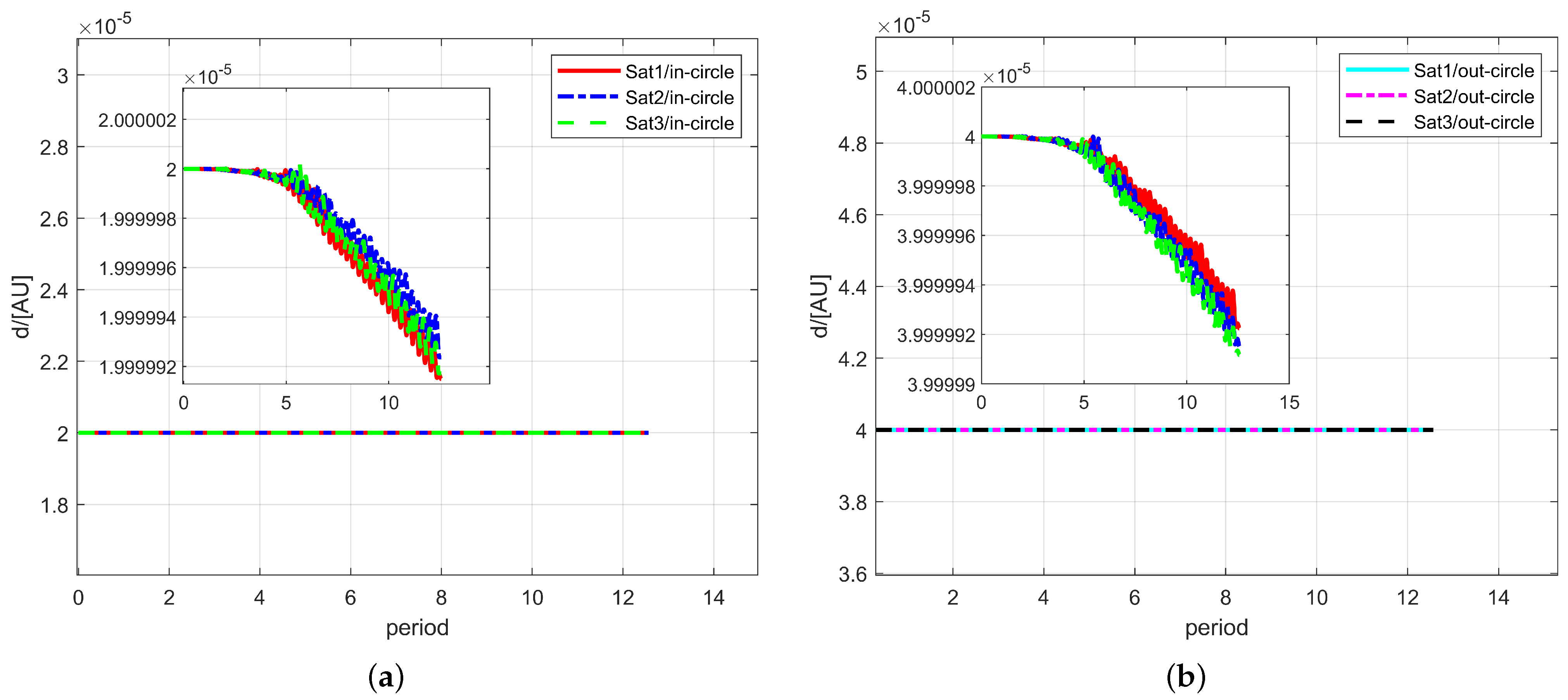
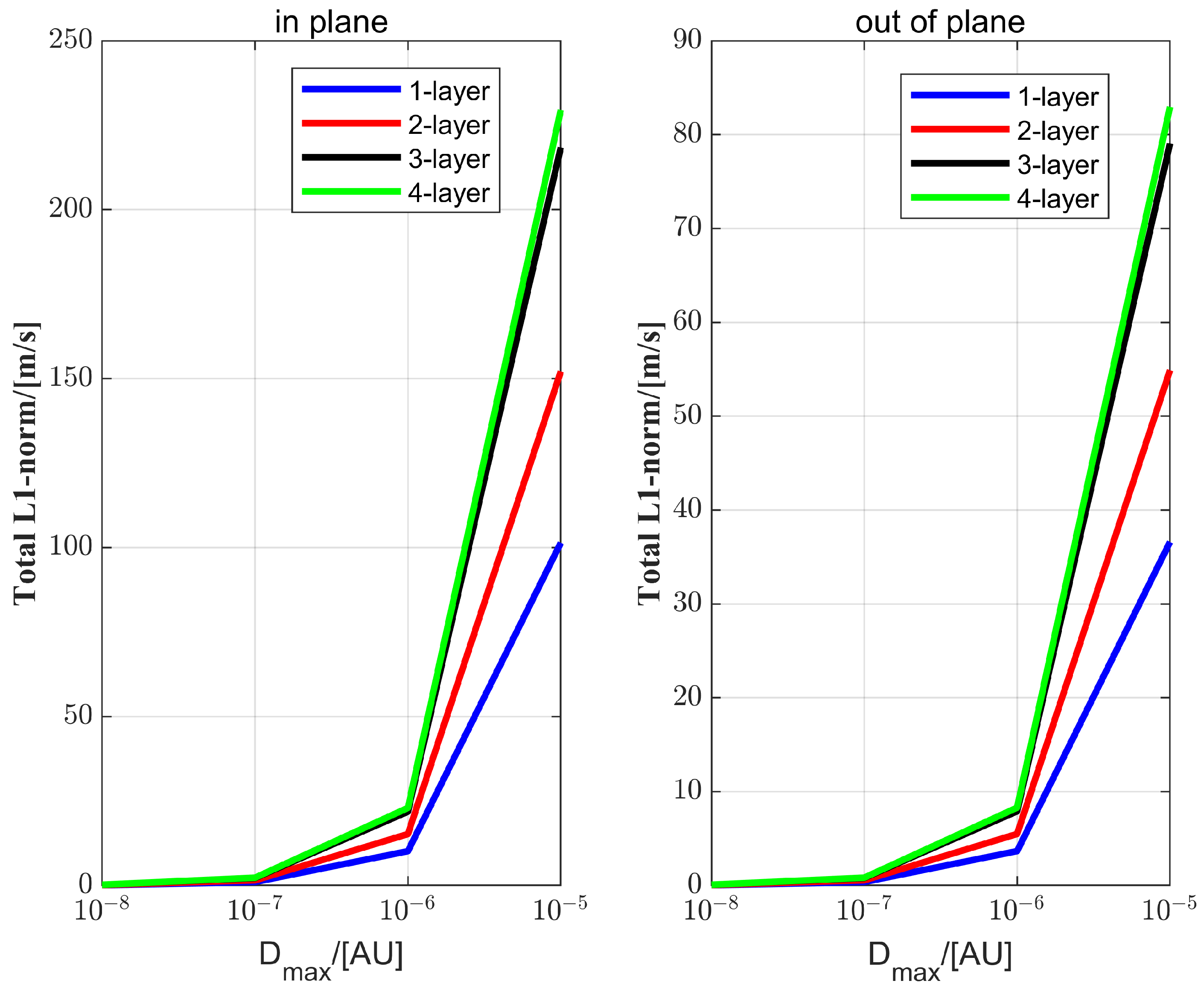
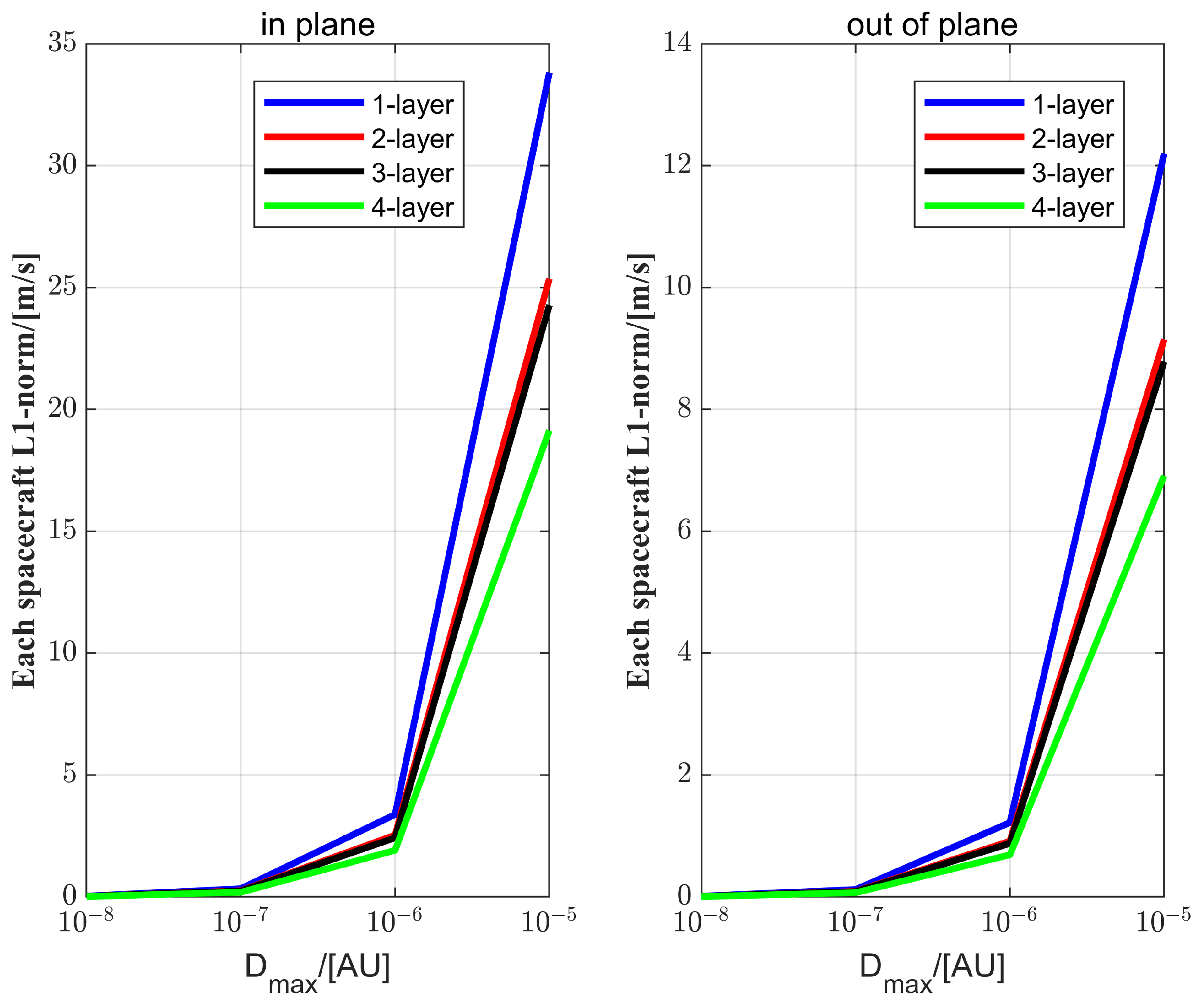
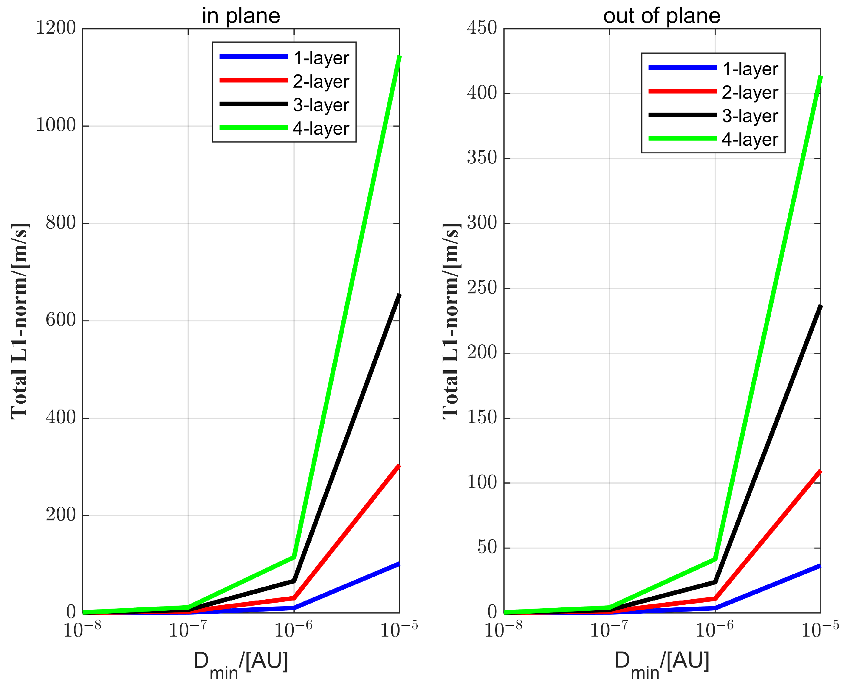
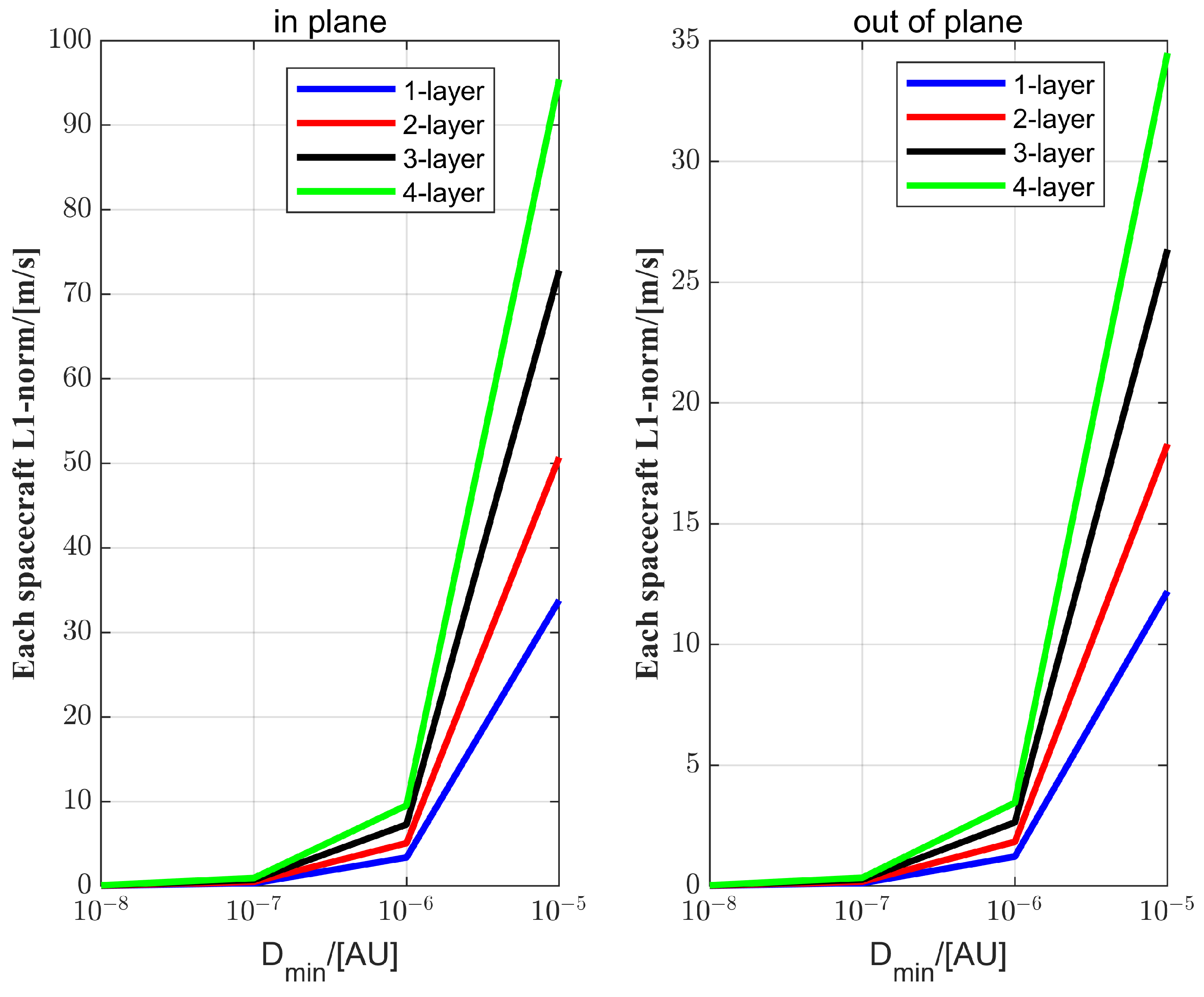
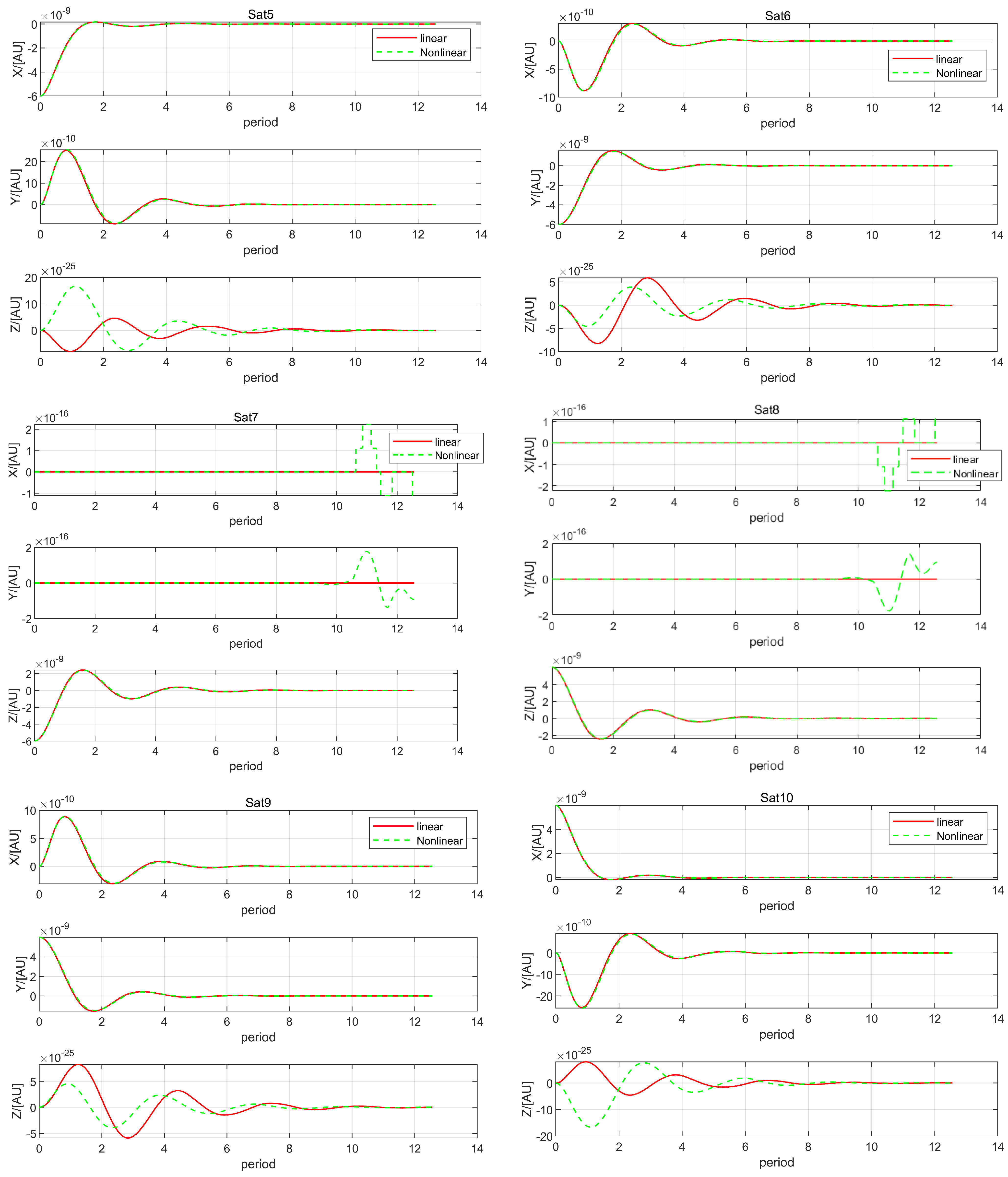
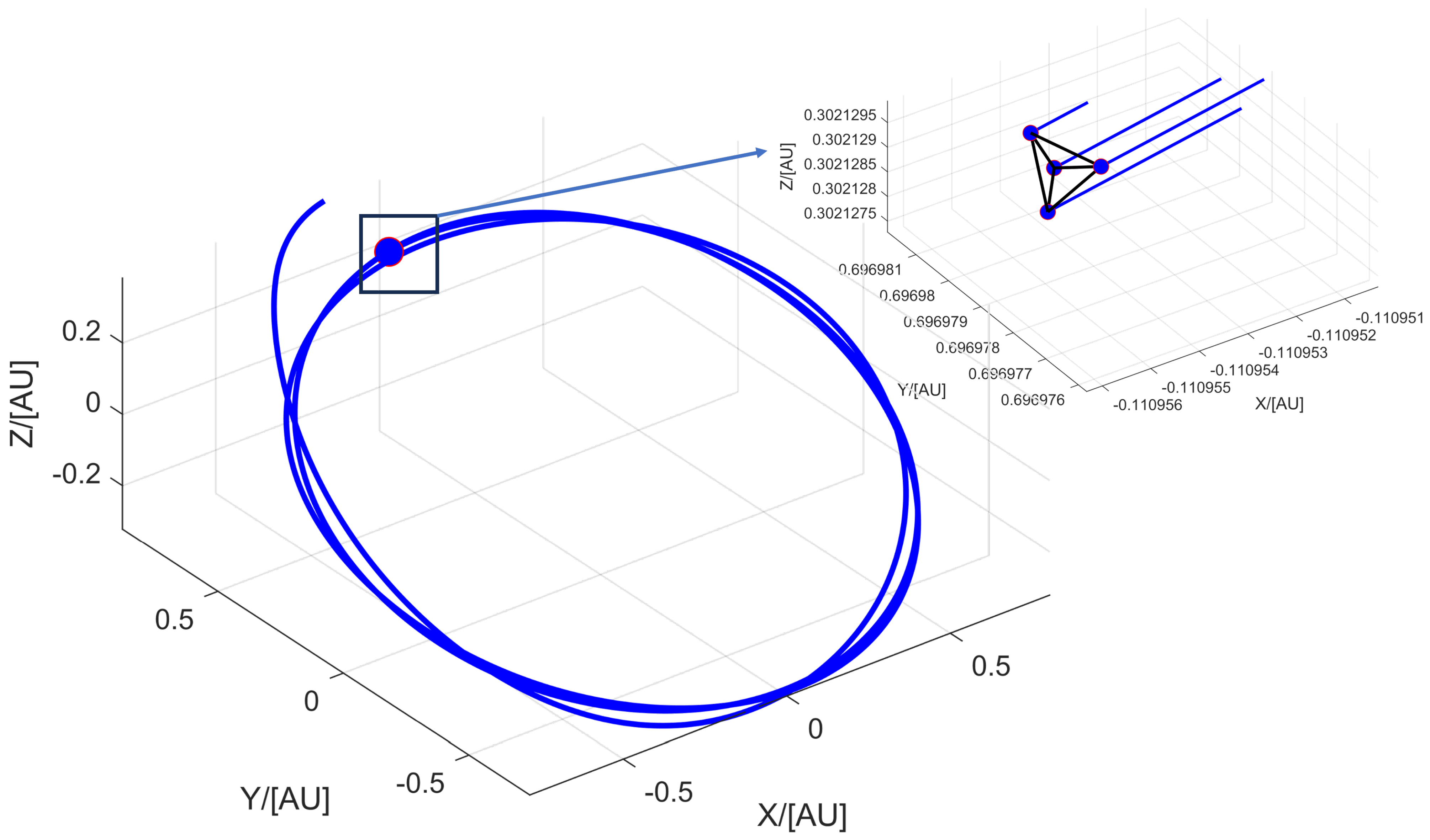
In this paper, to overcome the limitations of GWOs in specific orbits, a scientific observation mode and a non-scientific observation mode were proposed. For the non-scientific observation mode, the equilateral triangle array formation and equilateral tetrahedral array formation near Lagrange point $L_1$ were examined. To establish the array formations and maintain them, the tracking aspect of output regulation theory was employed. For the equilateral triangle array formation, the reference orbit was given by an exosystem. One-layer, two-layer, and three-layer triangle array formations were established and maintained. Simultaneously, the errors were reduced to zero through the control law, demonstrating the effectiveness of the control method. Next, the inner-edge length and the outer-edge length were fixed, and the formation fuel consumption was calculated. To observe GWs in different directions and avoid configuration/reconfiguration, the equilateral tetrahedral array formation was designed. The equilateral tetrahedral array formation was a fixed-point formation centered on Lagrange point $L_1$. To demonstrate the operation of the equilateral tetrahedral array formation, the trajectory of the array formation was given in the inertial frame in the ephemeris model. To show the configuration of the equilateral tetrahedral array formation, the configuration was given in a rotating frame in the ephemeris model, and it was well maintained by the control method.