Momentum-Based Adaptive Laws for Identification and Control

Abstract

In this paper, we develop momentum-based adaptive update laws for parameter identification and control to improve parameter estimation error convergence and control system performance for uncertain dynamical systems. Specifically, we introduce three novel continuous-time, momentum-based adaptive estimation and control algorithms and evaluate their effectiveness via several numerical examples. Our proposed adaptive architectures show faster parameter convergence rates as compared to the classical gradient descent and model reference adaptive control methods.

1. Introduction

One of the fundamental problems in feedback control design is the ability to address discrepancies between system models and real-world systems. To this end, adaptive control has been developed to address the problem of system uncertainty in control-system design [1,2,3,4]. In particular, adaptive control is based on constant linearly parameterized system uncertainty models of a known structure but unknown variation and, in the case of indirect adaptive control, combines an online parameter estimation algorithm with a control law to improve performance in the face of system uncertainties. More specifically, indirect adaptive controllers utilize parameter update laws to identify unknown system parameters and adjust feedback gains to account for system uncertainty.

The parameter estimation algorithms that have been typically used in adaptive control are predicated on two gradient descent type methods that update the system parameter errors in the direction that minimizes a prediction error for a specified cost function. Namely, for a gradient descent flow algorithm, the cost function involves an instantaneous prediction error between an estimated system output and the actual system output of the most recent data, whereas for an integral gradient descent algorithm the cost function captures an aggregate of the past prediction errors in an integral form while placing more emphasis on recent measurements [2].

Additionally, the recursive least squares (RLS) algorithm [2] has also been used for parameter estimation and has been shown to give superior convergence rates as compared to the classical gradient descent algorithms. RLS algorithms can be viewed as a gradient descent method with a time-varying learning rate [5]. For static (i.e., time-invariant) cost functions, momentum-based methods, also known as higher-order tuners, such as the Nesterov method, have been shown to achieve faster parameter error convergence as compared to traditional gradient descent algorithms [6]. Since faster convergence can lead to improved transient system performance, there has been a significant interest in extending momentum-based methods to time-varying cost functions, which naturally appear in adaptive control formulations [7,8,9].

Specifically, in [7] momentum-based architectures were merged with the standard gradient descent method using a variational approach to guarantee boundedness for the parameter estimation and model reference adaptive control problems involving time-varying regressors. Higher-order tuners were also shown to provide an additional degree of freedom in the design of adaptive control laws [10,11]. Given that integral gradient and recursive least squares algorithms provide superior noise rejection properties and improved system performance to that of standard gradient descent methods, there has been a recent interest in integrating momentum-based architectures into adaptive laws for parameter identification and control [5,7].

In this paper, we develop new continuous-time, momentum-based adaptive laws for identification and control by augmenting higher-order tuners into the integral gradient, recursive least squares and composite gradient algorithms. Specifically, in Section 2, we first review the existing gradient-based and momentum-based update laws and introduce three new higher-order tuner architectures. Next, in Section 3, we show how these update laws can be applied for parameter identification, and then, in Section 4, we introduce a momentum-based recursive least squares (MRLS) algorithm for model reference adaptive control. 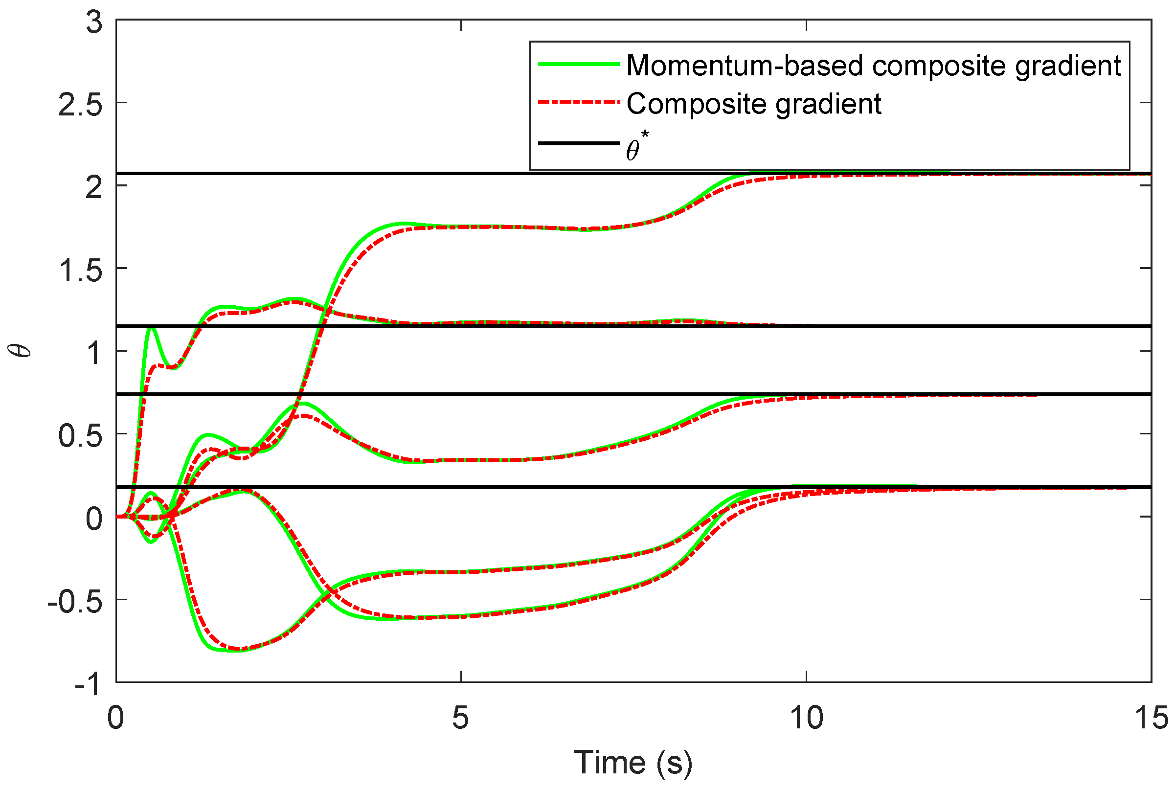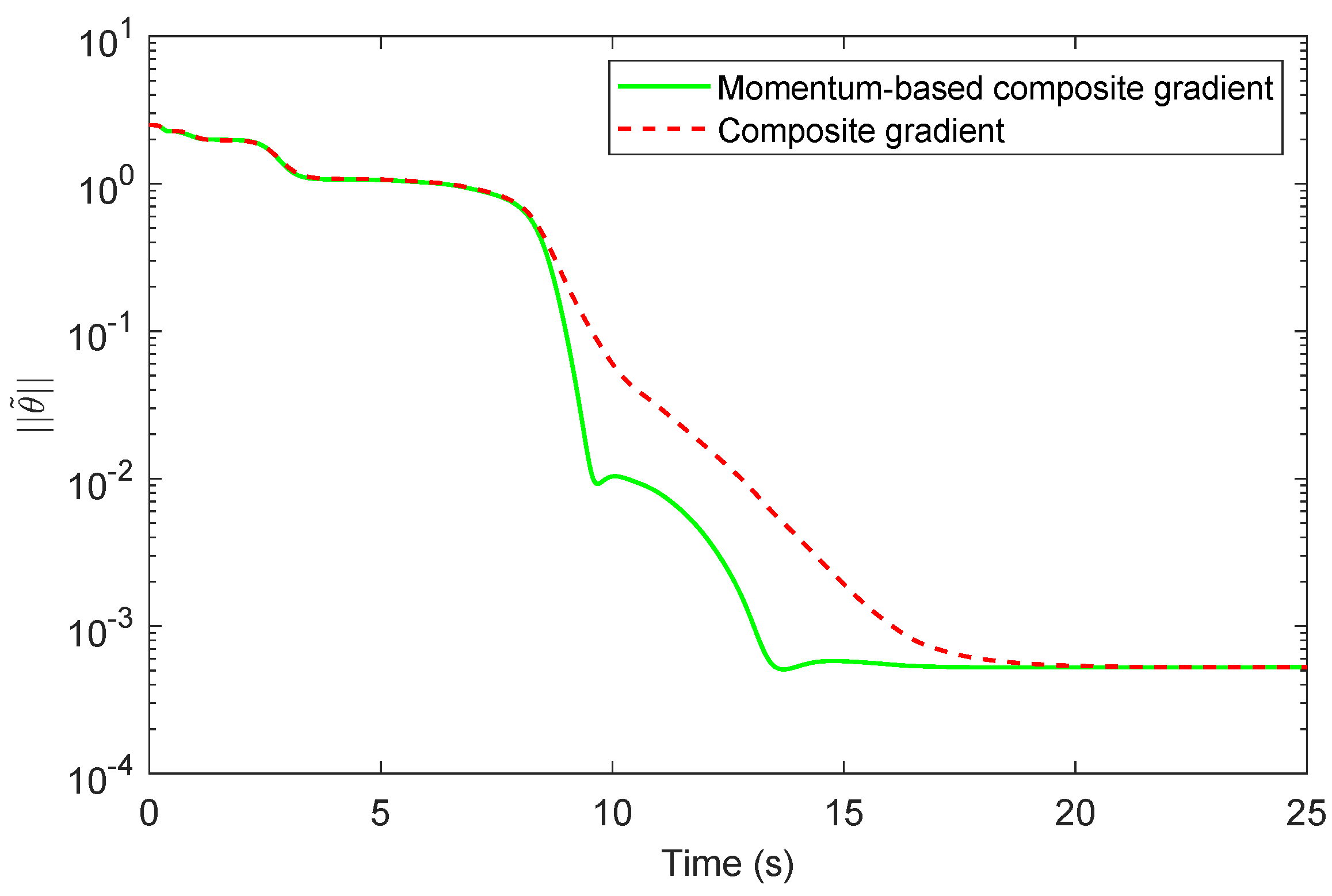Finally, Section 5 provides several numerical examples that highlight the improved parameter error convergence rate of the proposed momentum-based update laws.

The notation used in this paper is standard. Specifically, we write ${\mathbb{R}}^n$ to denote the set of $n\times 1$ column vectors, ${\mathbb{R}}^{n\times m}$ to denote the set of $n\times m$ real matrices, and ${(·)}^{\mathrm{T}}$ to denote transpose. The equi-induced 2-norm of a matrix $Q\in {\mathbb{R}}^{m\times n}$ is denoted as $\parallel Q\parallel \triangleq \sqrt{{\lambda }_{\max }\left(Q^{\mathrm{T}}Q\right)}={\sigma }_{\max }\left(Q\right),$ where ${\lambda }_{\max }(·)$ denotes the maximum eigenvalue and ${\sigma }_{\max }(·)$ denotes the maximum singular value. We write ${\lambda }_{\min }(·)$ (resp., ${\sigma }_{\min }(·)$) for the minimum eigenvalue (resp., singular value), ${\displaystyle \frac{\partial V}{\partial x}}\left(x\right)$ for the gradient of a scalar-valued function V with respect to a vector-valued variable x, and $\widehat{f}\left(s\right)$ for the Laplace transform of $f(·)$, that is $\widehat{f}\left(s\right)\triangleq \mathcal{L}\left\{f\left(t\right)\right\}={\int }_0^{\infty }{e}^{-st}f\left(t\right)\mathrm{d}t$. Finally, we write $\mathbb{R}\left(s\right)$ to denote the proper rational functions with coefficients in $\mathbb{R}$ (i.e., SISO proper rational transfer functions), $\mathbb{R}\left[s\right]$ to denote polynomials with real coefficients, ${\mathcal{L}}_2$ to denote the space of square-integrable Lebesgue measurable functions on $[0,\infty )$, and ${\mathcal{L}}_{\infty }$ to denote the space of bounded Lebesgue measurable functions on $[0,\infty )$.

2. From First-Order to Higher-Order Tuners for Parameter Estimation

Consider the system given by

$$\begin{array}{c}\hfill y\left(t\right)={\theta }^{*\mathrm{T}}\varphi \left(t\right),\end{array}$$

(1)

where, for $t\ge 0$, $y\left(t\right)\in \mathbb{R}$ is the system output, $\varphi \left(t\right)\in {\mathbb{R}}^N$ is a time-varying regressor vector, and ${\theta }^{*}\in {\mathbb{R}}^N$ is an unknown system parameter vector. Here we assume that $\varphi (·)$ is bounded, and hence, can be normalized via the scaling factor $1+\parallel \varphi \left(t\right)\parallel$ so that, with a minor abuse of notation, $\parallel \varphi \left(t\right)\parallel \le 1,t\ge 0$. Since ${\theta }^{*}$ is unknown, we design an estimator of the form $y_{\mathrm{e}}\left(t\right)=\theta {\left(t\right)}^{\mathrm{T}}\varphi \left(t\right)$, where $\theta \left(t\right),t\ge 0$, is an estimate of ${\theta }^{*}$, so that the prediction error between the estimated output $y_{\mathrm{e}}\left(t\right),t\ge 0$, and the actual system output $y\left(t\right),t\ge 0$, is given by

$$\begin{array}{cc}\hfill e\left(t\right)& \triangleq y_{\mathrm{e}}\left(t\right)-y\left(t\right)=\theta {\left(t\right)}^{\mathrm{T}}\varphi \left(t\right)-y\left(t\right)=\tilde{\theta }{\left(t\right)}^{\mathrm{T}}\varphi \left(t\right),\hfill \end{array}$$

(2)

where $\tilde{\theta }\left(t\right)\triangleq \theta \left(t\right)-{\theta }^{*}$ is the parameter estimation error.

For the error system (2), consider the quadratic loss cost function

$$\begin{array}{c}\hfill L(\theta ,t)={\displaystyle \frac{1}{2}}{e}^2\left(t\right)\end{array}$$

(3)

and note that the gradient of L with respect to the parameter estimate $\theta$ is given by ${\displaystyle \frac{\partial L(\theta ,t)}{\partial \theta }}=\varphi \left(t\right)e\left(t\right)$. In this case, the gradient flow algorithm is expressed as

$$\begin{array}{c}\hfill \dot{\theta }\left(t\right)=-\gamma {\displaystyle \frac{\partial L(\theta ,t)}{\partial \theta }}=-\gamma \varphi \left(t\right)e\left(t\right),\theta \left(0\right)={\theta }_0,t\ge 0,\end{array}$$

(4)

where $\gamma >0$ is a weighting gain parameter. As shown in [7], $e\in {\mathcal{L}}_{\infty }\cap {\mathcal{L}}_2$ for all $\gamma >0$.

It is well known that the rate of convergence for the gradient flow algorithm (4) can be slow [6]. However, if the regressor vector $\varphi (·)$ satisfies a persistency of the excitation condition, then $\theta \left(t\right)$ converges to ${\theta }^{*}$ exponentially with a convergence rate proportional to $\gamma$. Although in this case the convergence rate can improve significantly, large values of $\gamma$ can result in a stiff initial value problem for (4) necessitating progressively smaller sampling times for implementing (4) on a digital computer. Furthermore, small sampling times can increase the sensitivity of the adaptive law to measurement noise and modeling errors [2]. To address these limitations, momentum-based accelerated algorithms predicated on higher-order tuner laws are introduced in [7] to expedite parameter estimation error convergence.

In [12], an array of accelerated methods for continuous-time systems are derived using a Lagrangian variational formulation. Building on this work, [7] extends the variational framework of [12] to address a time-varying instantaneous quadratic loss function of the form given by (3). Specifically, a Lagrangian of the form

$$\begin{array}{c}\hfill \mathcal{L}(\theta ,\dot{\theta },t)=e^{{\int }_{t_0}^t\beta \mathcal{N}\left(s\right)\mathrm{d}s}{\displaystyle \frac{1}{2\beta \mathcal{N}\left(t\right)}}[{\dot{\theta }}^{\mathrm{T}}\left(t\right)\dot{\theta }\left(t\right)-\gamma \beta \mathcal{N}\left(t\right)e{\left(t\right)}^2]\end{array}$$

(5)

is introduced, where $\mathcal{N}\left(t\right)\triangleq 1+\mu \varphi {\left(t\right)}^{\mathrm{T}}\varphi \left(t\right),\mu >0$, $\beta >0$ is a friction coefficient, and $\gamma >0$, and the functional

$$\begin{array}{c}\hfill J\left(\theta \right)={\int }_{\mathbb{T}}\mathcal{L}(\theta ,\dot{\theta },t)\mathrm{d}s,\end{array}$$

(6)

where $\mathbb{T}$ is a finite-time interval, is considered. A necessary condition for $\theta$ minimizing (6) is shown in [7] to satisfy

$$\begin{array}{c}\hfill \ddot{\theta }\left(t\right)+\left[\beta \mathcal{N}\left(t\right)-{\displaystyle \frac{\dot{\mathcal{N}}\left(t\right)}{\mathcal{N}\left(t\right)}}\right]\dot{\theta }\left(t\right)=-\gamma \beta \mathcal{N}\left(t\right)\varphi \left(t\right)e\left(t\right),\dot{\theta }\left(0\right)={\dot{\theta }}_0,\theta \left(0\right)={\theta }_0,t\ge 0.\end{array}$$

(7)

Note that (7) can be rewritten as

$$\begin{array}{cc}\hfill \dot{\mathcal{V}}\left(t\right)& =-\gamma \varphi \left(t\right)e\left(t\right),\mathcal{V}\left(0\right)={\mathcal{V}}_0,t\ge 0,\hfill \end{array}$$

(8)

$$\begin{array}{cc}\hfill \dot{\theta }\left(t\right)& =-\beta [\theta \left(t\right)-\mathcal{V}\left(t\right)]\mathcal{N}\left(t\right),\theta \left(0\right)={\theta }_0,\hfill \end{array}$$

(9)

where $\mathcal{V}$ is an auxiliary parameter and ${\mathcal{V}}_0={\displaystyle \frac{1}{\mathcal{N}\left(0\right)\beta }}{\dot{\theta }}_0+{\theta }_0$. The stability properties of (8) and (9) are given in [7]. Taking the limiting case as $\beta \to \infty$, the gradient flow algorithm (4) can be recovered as a special case of (8) and (9).

Rather than relying solely on the instantaneous system measurement $y\left(t\right),t\ge 0$, the loss cost function (3) can be modified to incorporate a weighted sum of past system measurements. Specifically, we can consider loss cost functions in the form of (see [2])

$$\begin{array}{c}\hfill L(\theta ,t)={\displaystyle \frac{1}{2}}{\int }_0^t{e}^{-\nu (t-\tau )}{[y\left(\tau \right)-{\theta }^{\mathrm{T}}\left(t\right)\varphi \left(\tau \right)]}^2\mathrm{d}\tau ,\end{array}$$

(10)

where $\nu >0$ is a forgetting factor that prevents the degeneration of system information updates in some direction by placing more emphasis on the more recent measurements. In this case, the gradient of the loss cost function (10) is given by

$$\begin{array}{cc}\hfill {\displaystyle \frac{\partial L(\theta ,t)}{\partial \theta }}& ={\int }_0^t{e}^{-\nu (t-\tau )}[y\left(\tau \right)-{\theta }^{\mathrm{T}}\left(t\right)\varphi \left(\tau \right)]\varphi \left(\tau \right)\mathrm{d}\tau \hfill \\ \hfill & =R\left(t\right)\theta \left(t\right)+Q\left(t\right),\hfill \end{array}$$

(11)

where

$$\begin{array}{c}\hfill R\left(t\right)\triangleq {\int }_0^t{e}^{-\nu (t-\tau )}\varphi \left(\tau \right)\varphi {\left(\tau \right)}^{\mathrm{T}}\mathrm{d}\tau ,\end{array}$$

(12)

$$\begin{array}{c}\hfill Q\left(t\right)\triangleq {\int }_0^t{e}^{-\nu (t-\tau )}y\left(\tau \right)\varphi {\left(\tau \right)}^{\mathrm{T}}\mathrm{d}\tau .\end{array}$$

(13)

Now, setting

$$\begin{array}{c}\hfill \dot{\theta }\left(t\right)=-\gamma {\displaystyle \frac{\partial L(\theta ,t)}{\partial \theta }},\theta \left(0\right)={\theta }_0,t\ge 0,\end{array}$$

(14)

we obtain the integral gradient algorithm ([2])

$$\begin{array}{cc}\hfill \dot{\theta }\left(t\right)& =-\gamma [R\left(t\right)\theta \left(t\right)+Q\left(t\right)],\theta \left(0\right)={\theta }_0,t\ge 0,\hfill \end{array}$$

(15)

$$\begin{array}{cc}\hfill \dot{R}\left(t\right)& =-\nu R\left(t\right)+\varphi \left(t\right)\varphi {\left(t\right)}^{\mathrm{T}},R\left(0\right)=0,\hfill \end{array}$$

(16)

$$\begin{array}{cc}\hfill \dot{Q}\left(t\right)& =-\nu Q\left(t\right)-y\left(t\right)\varphi \left(t\right),Q\left(0\right)=0.\hfill \end{array}$$

(17)

The stability properties of (15)–(17) are addressed in [2] ([Thm. 3.6.7]).

Next, motivated by the variational formulation of [7] we introduce a momentum-based integral gradient algorithm. Specifically, defining the Lagrangian

$$\begin{array}{c}\hfill \mathcal{L}(\theta ,\dot{\theta },t)=e^{{\int }_{t_0}^t\beta {\mathcal{N}}_{\mathrm{i}}\left(s\right)\mathrm{d}s}{\displaystyle \frac{1}{\beta {\mathcal{N}}_{\mathrm{i}}\left(t\right)}}\left[{\displaystyle \frac{1}{2}}\dot{\theta }{\left(t\right)}^{\mathrm{T}}\dot{\theta }\left(t\right)-\gamma \beta {\mathcal{N}}_{\mathrm{i}}\left(t\right){\displaystyle \frac{1}{2}}{\int }_0^t{e}^{-\nu (t-\tau )}{(y\left(\tau \right)-{\theta }^{\mathrm{T}}\left(t\right)\varphi \left(t\right))}^2\mathrm{d}\tau \right],\end{array}$$

(18)

where ${\mathcal{N}}_{\mathrm{i}}\left(t\right)\triangleq 1+\mu \parallel R\left(t\right)\parallel ,\mu \ge 0$, and using the Euler-Lagrange equation, a necessary condition for $\theta$ minimizing (6) yields

$$\begin{array}{cc}\hfill \ddot{\theta }\left(t\right)+\left[\beta {\mathcal{N}}_{\mathrm{i}}\left(t\right)-{\displaystyle \frac{\dot{{\mathcal{N}}_{\mathrm{i}}}\left(t\right)}{{\mathcal{N}}_{\mathrm{i}}\left(t\right)}}\right]\dot{\theta }\left(t\right)& =-\gamma \beta {\mathcal{N}}_{\mathrm{i}}\left(t\right)[R\left(t\right)\theta \left(t\right)+Q\left(t\right)],\dot{\theta }\left(0\right)={\dot{\theta }}_0,\theta \left(0\right)={\theta }_0,\hfill \\ \hfill & t\ge 0,\hfill \end{array}$$

(19)

where, for $t\ge 0$, $R\left(t\right)$ and $Q\left(t\right)$ are given by (12) and (13). Note that (19) can be rewritten as

$$\begin{array}{cc}\hfill \dot{\mathcal{V}}\left(t\right)& =-\gamma [R\left(t\right)\theta \left(t\right)+Q\left(t\right)],\mathcal{V}\left(0\right)={\mathcal{V}}_0,t\ge 0,\hfill \end{array}$$

(20)

$$\begin{array}{cc}\hfill \dot{\theta }\left(t\right)& =-\beta [\theta \left(t\right)-\mathcal{V}\left(t\right)]{\mathcal{N}}_{\mathrm{i}}\left(t\right),\theta \left(0\right)={\theta }_0,\hfill \end{array}$$

(21)

$$\begin{array}{cc}\hfill \dot{R}\left(t\right)& =-\nu R\left(t\right)+\varphi \left(t\right)\varphi {\left(t\right)}^{\mathrm{T}},R\left(0\right)=0,\hfill \end{array}$$

(22)

$$\begin{array}{cc}\hfill \dot{Q}\left(t\right)& =-\nu Q\left(t\right)-y\left(t\right)\varphi \left(t\right),Q\left(0\right)=0,\hfill \end{array}$$

(23)

where $\mathcal{V}$ is an auxiliary parameter and ${\mathcal{V}}_0={\displaystyle \frac{1}{{\mathcal{N}}_{\mathrm{i}}\left(0\right)\beta }}{\dot{\theta }}_0+{\theta }_0$. Furthermore, (20) and (21) can be rewritten in terms of the parameter estimation error $\tilde{\theta }\left(t\right),t\ge 0$, and the auxiliary parameter estimation error $\tilde{\mathcal{V}}\left(t\right)\triangleq \mathcal{V}\left(t\right)-{\theta }^{*}$ as

$$\begin{array}{cc}\hfill \dot{\tilde{\mathcal{V}}}\left(t\right)& =-\gamma R\left(t\right)\tilde{\theta }\left(t\right),\tilde{\mathcal{V}}\left(0\right)={\tilde{\mathcal{V}}}_0,t\ge 0,\hfill \end{array}$$

(24)

$$\begin{array}{cc}\hfill \dot{\tilde{\theta }}\left(t\right)& =-\beta [\tilde{\theta }\left(t\right)-\tilde{\mathcal{V}}\left(t\right)]{\mathcal{N}}_{\mathrm{i}}\left(t\right),\tilde{\theta }\left(0\right)={\tilde{\theta }}_0.\hfill \end{array}$$

(25)

The following definition and lemmas are needed for the main results of this section.

Definition 1. 

A vector signal $\varphi :\mathbb{R}\to {\mathbb{R}}^N$ is persistently excited (PE) if there exist a positive constant ρ and a finite-time $\delta >0$ such that

$$\begin{array}{c}\hfill \rho I_N\le {\int }_t^{t+\delta }\varphi \left(\tau \right)\varphi {\left(\tau \right)}^{\mathrm{T}}d\tau ,t>0.\end{array}$$

(26)

Lemma 1. 

Consider the system (22). Then, the following statements hold:

$\left(i\right)$

$$\begin{array}{c}\hfill \parallel R\left(t\right)\parallel \le {\displaystyle \frac{1}{\nu }},t\ge 0.\end{array}$$

(27)

$\left(ii\right)$ If $\varphi (·)$ is persistently excited, then

$$\begin{array}{c}\hfill e^{-\nu \delta }\rho \le \parallel R\left(t\right)\parallel ,t\ge \delta .\end{array}$$

(28)

Proof. 

To show $\left(i\right)$, note that it follows from (12) and $\varphi \left(t\right)\varphi {\left(t\right)}^{\mathrm{T}}\le I_N,t\ge 0$, that

$$\begin{array}{cc}\hfill R\left(t\right)\le & {\int }_0^t{e}^{-\nu (t-\tau )}{I}_N\mathrm{d}\tau \le {\displaystyle \frac{1}{\nu }}{I}_N,t\ge 0,\hfill \end{array}$$

which proves (27). Next, to show ($ii)$, note that if $\varphi (·)$ is PE, then

$$\begin{array}{cc}\hfill R\left(t\right)& ={\int }_0^{t-\delta }{e}^{-\nu (t-\tau )}\varphi \left(\tau \right)\varphi {\left(\tau \right)}^{\mathrm{T}}\mathrm{d}\tau +{\int }_{t-\delta }^t{e}^{-\nu (t-\tau )}\varphi \left(\tau \right)\varphi {\left(\tau \right)}^{\mathrm{T}}\mathrm{d}\tau \hfill \\ \hfill & \ge {\int }_{t-\delta }^t{e}^{-\nu (t-\tau )}\varphi \left(\tau \right)\varphi {\left(\tau \right)}^{\mathrm{T}}\mathrm{d}\tau \hfill \\ \hfill & \ge e^{-\nu \delta }{\int }_{t-\delta }^t\varphi \left(\tau \right)\varphi {\left(\tau \right)}^{\mathrm{T}}\mathrm{d}\tau \hfill \\ \hfill & \ge e^{-\nu \delta }\rho I_N,t>\delta .\hfill \end{array}$$

(29)

This proves the lemma. □

Lemma 2 

([3]). Let $f:[0,\infty )\to {\mathbb{R}}^n$. If $f\in {\mathcal{L}}_2\cap {\mathcal{L}}_{\infty }$ and $\dot{f}\in {\mathcal{L}}_{\infty }$, then ${lim}_{t\to \infty }f\left(t\right)=0$.

Theorem 1. 

Let $\mu >{\displaystyle \frac{2\gamma }{\beta }}$, and consider the momentum-based integral gradient algorithm (20)–(23). Then, the following statements hold:

$\left(i\right)$$\theta \in {\mathcal{L}}_{\infty }$, $\dot{\theta },\dot{\mathcal{V}},\mathrm{and}(\theta -\mathcal{V})\in {\mathcal{L}}_{\infty }$, and ${lim}_{t\to \infty }\dot{\theta }\left(t\right)=0$.

$\left(ii\right)$ If $\varphi (·)$ is persistently excited, then $\theta \left(t\right)$ converges to ${\theta }^{*}$ exponentially as $t\to \infty$ with a convergence rate of ${\displaystyle \frac{a}{2}}$, where $a\triangleq min\{e^{-\nu \delta }\rho \gamma ,2\beta \}$.

Proof. 

To show $\left(i\right)$, consider the positive-definite function $V(\tilde{\mathcal{V}},\tilde{\theta })\triangleq {\tilde{\mathcal{V}}}^{\mathrm{T}}\tilde{\mathcal{V}}+{(\tilde{\theta }-\tilde{\mathcal{V}})}^{\mathrm{T}}(\tilde{\theta }-\tilde{\mathcal{V}})$ and note that

$$\begin{array}{cc}\hfill \dot{V}(\tilde{\mathcal{V}},\tilde{\theta },t)& =2{\tilde{\mathcal{V}}}^{\mathrm{T}}\dot{\tilde{\mathcal{V}}}+2{(\tilde{\theta }-\tilde{\mathcal{V}})}^{\mathrm{T}}(\dot{\tilde{\theta }}-\dot{\tilde{\mathcal{V}}})\hfill \\ \hfill & =-2\gamma {\tilde{\mathcal{V}}}^{\mathrm{T}}R\left(t\right)\tilde{\theta }-2\beta \parallel \tilde{\theta }-\tilde{\mathcal{V}}{\parallel }^2(1+\mu \parallel R\left(t\right)\parallel )+2\gamma {(\tilde{\theta }-\tilde{\mathcal{V}})}^{\mathrm{T}}R\left(t\right)\tilde{\theta }\hfill \\ \hfill & \le -2\gamma {\tilde{\theta }}^{\mathrm{T}}R\left(t\right)\tilde{\theta }-2\beta \parallel \tilde{\theta }-\tilde{\mathcal{V}}{\parallel }^2(1+\mu \parallel R\left(t\right)\parallel )+4\gamma \parallel {(\tilde{\theta }-\tilde{\mathcal{V}})}^{\mathrm{T}}{R}^{{\displaystyle \frac{1}{2}}}\left(t\right)\parallel \parallel R^{{\displaystyle \frac{1}{2}}}\left(t\right)\tilde{\theta }\parallel \hfill \\ \hfill & \le -2\gamma {\tilde{\theta }}^{\mathrm{T}}R\left(t\right)\tilde{\theta }-2\beta \parallel \tilde{\theta }-\tilde{\mathcal{V}}{\parallel }^2(1+\mu \parallel R\left(t\right)\parallel )+4\gamma \parallel {(\tilde{\theta }-\tilde{\mathcal{V}})}^{\mathrm{T}}{R}^{{\displaystyle \frac{1}{2}}}\left(t\right)\parallel \parallel R^{{\displaystyle \frac{1}{2}}}\left(t\right)\tilde{\theta }\parallel \hfill \\ \hfill & \le -\gamma {\tilde{\theta }}^{\mathrm{T}}R\left(t\right)\tilde{\theta }-2\beta {\parallel \tilde{\theta }-\tilde{\mathcal{V}}\parallel }^2-\gamma {\left[\parallel R^{{\displaystyle \frac{1}{2}}}\left(t\right)\tilde{\theta }\parallel -2\parallel {(\tilde{\theta }-\tilde{\mathcal{V}})}^{\mathrm{T}}{R}^{{\displaystyle \frac{1}{2}}}\left(t\right)\parallel \right]}^2\hfill \\ \hfill & \le -\gamma {\tilde{\theta }}^{\mathrm{T}}R\left(t\right)\tilde{\theta }-2\beta {\parallel \tilde{\theta }-\tilde{\mathcal{V}}\parallel }^2,\hfill \end{array}$$

(30)

which, since $R\left(t\right)\ge 0,t\ge 0$, implies $\dot{V}(\tilde{\mathcal{V}},\tilde{\theta },t)\le 0,t\ge 0$. Thus, $V,\tilde{\theta },$ and $(\tilde{\theta }-\tilde{\mathcal{V}})\in {\mathcal{L}}_{\infty }$.

Next, integrating $\dot{V}$ over $[0,\infty )$ yields

$$\begin{array}{c}\hfill {\int }_0^{\infty }{\parallel R^{{\displaystyle \frac{1}{2}}}\left(\tau \right)\tilde{\theta }\left(\tau \right)\parallel }^2\mathrm{d}\tau \le V({\tilde{\mathcal{V}}}_0,{\tilde{\theta }}_0,0)-\underset{t\to \infty }{lim}V(\tilde{\mathcal{V}}\left(t\right),\tilde{\theta }\left(t\right),t)<\infty ,\end{array}$$

and hence, $\parallel R^{{\displaystyle \frac{1}{2}}}\tilde{\theta }\parallel \in {\mathcal{L}}_2$. Similarly, $\parallel \tilde{\theta }-\tilde{\mathcal{V}}{\parallel }^2\in {\mathcal{L}}_2$, and hence, $(\tilde{\theta }-\tilde{\mathcal{V}})\in {\mathcal{L}}_{\infty }\cap {\mathcal{L}}_2$. Since (27) implies that $\parallel R\parallel \in {\mathcal{L}}_{\infty }$, it follows that $\parallel R^{{\displaystyle \frac{1}{2}}}\tilde{\theta }\parallel \in {\mathcal{L}}_{\infty }$. Now, it follows from (24) and (25) that $\dot{\tilde{\mathcal{V}}}$, $\dot{\tilde{\theta }}\in {\mathcal{L}}_{\infty }\cap {\mathcal{L}}_2$. Finally, since $\parallel \dot{R}\parallel \in {\mathcal{L}}_{\infty }$, it follows that $\ddot{\tilde{\mathcal{V}}}$, $\ddot{\tilde{\theta }}\in {\mathcal{L}}_{\infty }$, and, by Lemma 2, it follows that ${lim}_{t\to \infty }\parallel \dot{\theta }\left(t\right)\parallel =0$.

Next, to show ($ii)$, it follows from (28) and (30) that

$$\begin{array}{cc}\hfill \dot{V}(\tilde{\mathcal{V}},\tilde{\theta },t)& \le -min\{e^{-\nu \delta }\rho \gamma ,2\beta \}V(\tilde{\mathcal{V}},\tilde{\theta }),t\ge \delta ,\hfill \end{array}$$

which implies that

$$\begin{array}{c}\hfill V(\tilde{\mathcal{V}}\left(t\right),\tilde{\theta }\left(t\right))\le V({\tilde{\mathcal{V}}}_0,{\tilde{\theta }}_0)e^{-at},t\ge \delta .\end{array}$$

(31)

Now, (31) implies that, for all $t\ge \delta$,

$$\begin{array}{cc}\hfill \parallel \tilde{\mathcal{V}}\left(t\right)\parallel & \le \sqrt{V({\tilde{\mathcal{V}}}_0,{\tilde{\theta }}_0)}{e}^{-{\displaystyle \frac{a}{2}}t},\hfill \\ \hfill \parallel \tilde{\theta }\left(t\right)-\tilde{\mathcal{V}}\left(t\right)\parallel & \le \sqrt{V({\tilde{\mathcal{V}}}_0,{\tilde{\theta }}_0)}{e}^{-{\displaystyle \frac{a}{2}}t},\hfill \end{array}$$

and hence, using the triangle inequality $\parallel \tilde{\theta }\parallel -\parallel \tilde{\mathcal{V}}\parallel \le \parallel \tilde{\theta }-\tilde{\mathcal{V}}\parallel$, it follows that

$$\begin{array}{c}\hfill \parallel \tilde{\theta }\left(t\right)\parallel \le 2\sqrt{V({\tilde{\mathcal{V}}}_0,{\tilde{\theta }}_0)}{e}^{-{\displaystyle \frac{a}{2}}t},t\ge \delta ,\end{array}$$

(32)

which proves that $\tilde{\theta }\left(t\right)$ converges to 0 exponentially as $t\to \infty$ with a convergence rate of ${\displaystyle \frac{a}{2}}$. □

Remark 1. 

Note that unlike gradient flow and recursive least squares algorithms, the momentum-based integral gradient algorithm (20)–(23) does not require the assumption that $\dot{\varphi }(·)\in {\mathcal{L}}_{\infty }$ in order to guarantee that ${lim}_{t\to \infty }\dot{\theta }\left(t\right)=0$ [7].

Remark 2. 

Note that a time-varying forgetting factor can also be employed in (22) and (23). In this case, the PE condition can be replaced with a less restrictive excitation condition where (26) holds for a fixed-time t and not for all $t\ge 0$ [13].

Next, we consider the cost function

$$\begin{array}{cc}\hfill J(\theta ,t)& ={\int }_0^t{(y\left(\tau \right)-\varphi {\left(\tau \right)}^{\mathrm{T}}\theta \left(\tau \right))}^2-{(\theta \left(t\right)-\theta \left(\tau \right))}^{\mathrm{T}}F\left(\tau \right)(\theta \left(t\right)-\theta \left(\tau \right))\mathrm{d}\tau \hfill \\ \hfill & +{(\theta \left(t\right)-\theta \left(0\right))}^{\mathrm{T}}{\Gamma }_0(\theta \left(t\right)-\theta \left(0\right)),\hfill \end{array}$$

(33)

where for all $t\ge 0,F\left(t\right)$ is an $N\times N$ nonnegative-definite matrix function called the general forgetting matrix and ${\Gamma }_0$ is an $N\times N$ positive-definite matrix. It can be shown that a necessary condition for $\theta$ minimizing (33) gives the recursive least squares algorithm ([14])

$$\begin{array}{cc}\hfill \dot{\theta }\left(t\right)& =-\Gamma \left(t\right)\varphi \left(t\right)e\left(t\right),\theta \left(0\right)={\theta }_0,t\ge 0,\hfill \end{array}$$

(34)

$$\begin{array}{cc}\hfill \dot{\Gamma }\left(t\right)& =-\Gamma \left(t\right)[\varphi \left(t\right)\varphi {\left(t\right)}^{\mathrm{T}}-F\left(t\right)]\Gamma \left(t\right),\Gamma \left(0\right)={\Gamma }_0.\hfill \end{array}$$

(35)

Note that setting $F\left(t\right)\equiv 0$ and $F\left(t\right)=\nu H\left(t\right)=\nu {\Gamma }^{-1}\left(t\right)$, where $\Gamma \left(t\right)$ is positive-definite for all $t\ge 0$ (see [2]), we recover, respectively, the pure recursive least squares and the recursive least squares with exponential forgetting algorithms discussed in [2].

Note that the RLS algorithms (34) and (35) do not involve a gradient flow architecture, and the variational formulation cannot be used to generate a momentum-based recursive least squares (MRLS) algorithm. Despite this fact, higher-order tuner laws can still be incorporated into the RLS architecture to give the MRLS architecture

$$\begin{array}{cc}\hfill \dot{\mathcal{V}}\left(t\right)& =-\Gamma \left(t\right)\varphi \left(t\right)e\left(t\right),\mathcal{V}\left(0\right)={\mathcal{V}}_0,t\ge 0,\hfill \end{array}$$

(36)

$$\begin{array}{cc}\hfill \dot{\theta }\left(t\right)& =-\beta (\theta \left(t\right)-\mathcal{V}\left(t\right)){\mathcal{N}}_{\mathrm{r}}\left(t\right),\theta \left(0\right)={\theta }_0,\hfill \end{array}$$

(37)

$$\begin{array}{cc}\hfill \dot{\Gamma }\left(t\right)& =-\Gamma \left(t\right)[\varphi \left(t\right)\varphi {\left(t\right)}^{\mathrm{T}}-F\left(t\right)]\Gamma \left(t\right),\Gamma \left(0\right)={\Gamma }_0,\hfill \end{array}$$

(38)

where $\beta >0$ and ${\mathcal{N}}_{\mathrm{r}}\left(t\right)\triangleq 1+\mu \varphi {\left(t\right)}^{\mathrm{T}}\Gamma \left(t\right)\varphi \left(t\right)=1+\mu {\parallel {\Gamma }^{{\displaystyle \frac{1}{2}}}\left(t\right)\varphi \left(t\right)\parallel }^2$, $\mu >0$. Note that (36) and (37) can be rewritten as

$$\begin{array}{cc}\hfill \dot{\tilde{\mathcal{V}}}\left(t\right)& =-\Gamma \left(t\right)\varphi \left(t\right)e\left(t\right),\tilde{\mathcal{V}}\left(0\right)={\tilde{\mathcal{V}}}_0,t\ge 0,\hfill \end{array}$$

(39)

$$\begin{array}{cc}\hfill \dot{\tilde{\theta }}\left(t\right)& =-\beta (\tilde{\theta }\left(t\right)-\tilde{\mathcal{V}}\left(t\right)){\mathcal{N}}_{\mathrm{r}}\left(t\right),\tilde{\theta }\left(0\right)={\tilde{\theta }}_0.\hfill \end{array}$$

(40)

Noting that $H\left(t\right)={\Gamma }^{-1}\left(t\right)$ and using the fact that

$$\begin{array}{c}\hfill {\displaystyle \frac{\mathrm{d}H\left(t\right)\Gamma \left(t\right)}{\mathrm{d}t}}={\displaystyle \frac{\mathrm{d}{I}_n}{\mathrm{d}t}}=0=\dot{H}\left(t\right)\Gamma \left(t\right)+H\left(t\right)\dot{\Gamma }\left(t\right),\end{array}$$

(41)

it follows that

$$\begin{array}{cc}\hfill \dot{H}\left(t\right)& =-F\left(t\right)+\varphi \left(t\right)\varphi {\left(t\right)}^{\mathrm{T}},H\left(0\right)={\Gamma }_0^{-1},t\ge 0.\hfill \end{array}$$

(42)

Lemma 3. 

Consider the system (42) with $F\left(t\right)=\nu H\left(t\right)$. Then, the following statements hold:

$\left(i\right)$

$$\begin{array}{c}\hfill \parallel H\left(t\right)\parallel \le {\alpha }_2,t\ge 0,\end{array}$$

(43)

where ${\alpha }_2\triangleq {\lambda }_{\max }\left({\Gamma }_0^{-1}\right)+{\displaystyle \frac{1}{\nu }}$.

$\left(ii\right)$ If $\varphi (·)$ is persistently excited, then

$$\begin{array}{c}\hfill {\alpha }_1\le \parallel H\left(t\right)\parallel ,t\ge 0,\end{array}$$

(44)

where ${\alpha }_1\triangleq min\{e^{-\nu \delta }\rho ,e^{-\nu \delta }{\lambda }_{\min }\left({\Gamma }_0^{-1}\right)\}$.

Proof. 

To show $\left(i\right)$, note that it follows from (42) with $F\left(t\right)=\nu H\left(t\right)$ that

$$H\left(t\right)=e^{-\nu t}{\Gamma }_0^{-1}+{\int }_0^t{e}^{-\nu (t-\tau )}\varphi \left(\tau \right)\varphi {\left(\tau \right)}^{\mathrm{T}}\mathrm{d}\tau .$$

(45)

Now, using $\varphi \left(t\right)\varphi {\left(t\right)}^{\mathrm{T}}\le I_N,t\ge 0,$ yields

$$\begin{array}{cc}\hfill H\left(t\right)& \le {\Gamma }_0^{-1}+{\int }_0^t{e}^{-\nu (t-\tau )}{I}_N\mathrm{d}\tau \le {\lambda }_{\max }\left({\Gamma }_0^{-1}\right)I_N+{\displaystyle \frac{1}{\nu }}{I}_N,t\ge 0,\hfill \end{array}$$

which proves (43).

Next, to show ($ii)$, note that if $\varphi (·)$ is PE, then

$$H\left(t\right)\ge e^{-\nu t}{\Gamma }_0^{-1}\ge e^{-\nu \delta }{\lambda }_{\min }\left({\Gamma }_0^{-1}\right)I_N,0\le t<\delta ,$$

(46)

and

$$H\left(t\right)\ge e^{-\nu \delta }{\int }_{t-\delta }^t\varphi \left(\tau \right)\varphi {\left(\tau \right)}^{\mathrm{T}}\mathrm{d}\tau \ge e^{-\nu \delta }\rho I_N,t>\delta .$$

(47)

Thus,

$$\begin{array}{c}\hfill {\alpha }_1\le \parallel H\left(t\right)\parallel ,t\ge 0.\end{array}$$

(48)

This proves the lemma. □

Theorem 2. 

Let $\mu >{\displaystyle \frac{2}{\beta }}$, and consider the momentum-based recursive least squares algorithm (36)–(38). Then, $e(·)$ given by (2) satisfies $e\in {\mathcal{L}}_2$. Furthermore, the following statements hold:

$\left(i\right)$ If there exists ${\alpha }_1>0$ such that (44) holds, then $\mathcal{V}$, $\theta \in {\mathcal{L}}_{\infty }$. If, in addition, $\dot{\varphi }\in {\mathcal{L}}_{\infty }$, then ${lim}_{t\to \infty }\dot{\theta }\left(t\right)=0$ and ${lim}_{t\to \infty }e\left(t\right)=0$.

$\left(ii\right)$ If $F\left(t\right)=\nu H\left(t\right)$ and $\varphi (·)$ is persistently excited, then the zero solution $(\tilde{\mathcal{V}}\left(t\right),\tilde{\theta }\left(t\right))\equiv (0,0)$ to (39) and (40) is exponentially stable.

Proof. 

Consider the function $V(\tilde{\mathcal{V}},\tilde{\theta },t)\triangleq {\tilde{\mathcal{V}}}^{\mathrm{T}}H\left(t\right)\tilde{\mathcal{V}}+{(\tilde{\theta }-\tilde{\mathcal{V}})}^{\mathrm{T}}H\left(t\right)(\tilde{\theta }-\tilde{\mathcal{V}})$ and note that

$$\begin{array}{cc}\hfill & \dot{V}(\tilde{\mathcal{V}},\tilde{\theta },t)\hfill \\ \hfill & =2{\tilde{\mathcal{V}}}^{\mathrm{T}}H\left(t\right)\dot{\tilde{\mathcal{V}}}+{\tilde{\mathcal{V}}}^{\mathrm{T}}\dot{H}\left(t\right)\tilde{\mathcal{V}}+2{(\tilde{\theta }-\tilde{\mathcal{V}})}^{\mathrm{T}}H\left(t\right)(\dot{\tilde{\theta }}-\dot{\tilde{\mathcal{V}}})+{(\tilde{\theta }-\tilde{\mathcal{V}})}^{\mathrm{T}}\dot{H}\left(t\right)(\tilde{\theta }-\tilde{\mathcal{V}})\hfill \\ \hfill & =-2{\tilde{\mathcal{V}}}^{\mathrm{T}}H\left(t\right)\Gamma \left(t\right)\varphi \left(t\right)e+{\tilde{\mathcal{V}}}^{\mathrm{T}}[-\nu H\left(t\right)+\varphi \left(t\right)\varphi {\left(t\right)}^{\mathrm{T}}]\tilde{\mathcal{V}}-2\beta {(\tilde{\theta }-\tilde{\mathcal{V}})}^{\mathrm{T}}H\left(t\right)(\tilde{\theta }-\tilde{\mathcal{V}}){\mathcal{N}}_{\mathrm{r}}\left(t\right)\hfill \\ \hfill & -2\beta {(\tilde{\theta }-\tilde{\mathcal{V}})}^{\mathrm{T}}H\left(t\right)\Gamma \left(t\right)\varphi \left(t\right)e+{(\tilde{\theta }-\tilde{\mathcal{V}})}^{\mathrm{T}}[-\nu H\left(t\right)+\varphi \left(t\right)\varphi {\left(t\right)}^{\mathrm{T}}](\tilde{\theta }-\tilde{\mathcal{V}})\hfill \\ \hfill & =-{\tilde{\mathcal{V}}}^{\mathrm{T}}F\left(t\right)\tilde{\mathcal{V}}-\nu {(\tilde{\theta }-\tilde{\mathcal{V}})}^{\mathrm{T}}F\left(t\right)(\tilde{\theta }-\tilde{\mathcal{V}})-2{\tilde{\mathcal{V}}}^{\mathrm{T}}\varphi \left(t\right)\varphi {\left(t\right)}^{\mathrm{T}}\tilde{\theta }+{\tilde{\mathcal{V}}}^{\mathrm{T}}\varphi \left(t\right)\varphi {\left(t\right)}^{\mathrm{T}}\tilde{\mathcal{V}}\hfill \\ \hfill & -2\beta {(\tilde{\theta }-\tilde{\mathcal{V}})}^{\mathrm{T}}H\left(t\right)(\tilde{\theta }-\tilde{\mathcal{V}}){\mathcal{N}}_{\mathrm{r}}\left(t\right)-2\beta {(\tilde{\theta }-\tilde{\mathcal{V}})}^{\mathrm{T}}\varphi \left(t\right)\varphi {\left(t\right)}^{\mathrm{T}}\tilde{\theta }\hfill \\ \hfill & +{(\tilde{\theta }-\tilde{\mathcal{V}})}^{\mathrm{T}}\varphi \left(t\right)\varphi {\left(t\right)}^{\mathrm{T}}(\tilde{\theta }-\tilde{\mathcal{V}})\hfill \\ \hfill & =-{\tilde{\mathcal{V}}}^{\mathrm{T}}F\left(t\right)\tilde{\mathcal{V}}-\nu {(\tilde{\theta }-\tilde{\mathcal{V}})}^{\mathrm{T}}F\left(t\right)(\tilde{\theta }-\tilde{\mathcal{V}})+{(\tilde{\theta }-\tilde{\mathcal{V}})}^{\mathrm{T}}\varphi \left(t\right)\varphi {\left(t\right)}^{\mathrm{T}}(\tilde{\theta }-\tilde{\mathcal{V}})-2e^2\hfill \\ \hfill & -2\beta {(\tilde{\theta }-\tilde{\mathcal{V}})}^{\mathrm{T}}H\left(t\right)(\tilde{\theta }-\tilde{\mathcal{V}}){\mathcal{N}}_{\mathrm{r}}\left(t\right)-2\beta {(\tilde{\theta }-\tilde{\mathcal{V}})}^{\mathrm{T}}\varphi \left(t\right)\varphi {\left(t\right)}^{\mathrm{T}}\tilde{\theta }\hfill \\ \hfill & +{(\tilde{\theta }-\tilde{\mathcal{V}})}^{\mathrm{T}}\varphi \left(t\right)\varphi {\left(t\right)}^{\mathrm{T}}(\tilde{\theta }-\tilde{\mathcal{V}})\hfill \\ \hfill & =-{\tilde{\mathcal{V}}}^{\mathrm{T}}F\left(t\right)\tilde{\mathcal{V}}-\nu {(\tilde{\theta }-\tilde{\mathcal{V}})}^{\mathrm{T}}F\left(t\right)(\tilde{\theta }-\tilde{\mathcal{V}})+2{\parallel {(\tilde{\theta }-\tilde{\mathcal{V}})}^{\mathrm{T}}\varphi \left(t\right)\parallel }^2-2e^2\hfill \\ \hfill & -2\beta {(\tilde{\theta }-\tilde{\mathcal{V}})}^{\mathrm{T}}H\left(t\right)(\tilde{\theta }-\tilde{\mathcal{V}}){\mathcal{N}}_{\mathrm{r}}\left(t\right)-2{(\tilde{\theta }-\tilde{\mathcal{V}})}^{\mathrm{T}}\varphi \left(t\right)\varphi {\left(t\right)}^{\mathrm{T}}\tilde{\theta }\hfill \\ \hfill & \le -{\tilde{\mathcal{V}}}^{\mathrm{T}}F\left(t\right)\tilde{\mathcal{V}}-\nu {(\tilde{\theta }-\tilde{\mathcal{V}})}^{\mathrm{T}}F\left(t\right)(\tilde{\theta }-\tilde{\mathcal{V}})+2{\parallel {(\tilde{\theta }-\tilde{\mathcal{V}})}^{\mathrm{T}}\varphi \left(t\right)\parallel }^2-2e^2\hfill \\ \hfill & -2\beta {(\tilde{\theta }-\tilde{\mathcal{V}})}^{\mathrm{T}}H\left(t\right)(\tilde{\theta }-\tilde{\mathcal{V}})(1+\mu \parallel {\Gamma }^{{\displaystyle \frac{1}{2}}}\left(t\right)\varphi \left(t\right)\parallel )+2\parallel {(\tilde{\theta }-\tilde{\mathcal{V}})}^{\mathrm{T}}\varphi \left(t\right)\parallel |e|.\hfill \end{array}$$

Now, by the Cauchy–Schwarz inequality,

$$\begin{array}{c}\hfill \parallel {(\tilde{\theta }-\tilde{\mathcal{V}})}^{\mathrm{T}}\varphi \left(t\right)\parallel =\parallel {(\tilde{\theta }-\tilde{\mathcal{V}})}^{\mathrm{T}}{H}^{{\displaystyle \frac{1}{2}}}\left(t\right){\Gamma }^{{\displaystyle \frac{1}{2}}}\left(t\right)\varphi \left(t\right)\parallel \le \parallel H^{{\displaystyle \frac{1}{2}}}\left(t\right)(\tilde{\theta }-\tilde{\mathcal{V}})\parallel \parallel {\Gamma }^{{\displaystyle \frac{1}{2}}}\left(t\right)\varphi \left(t\right)\parallel ,\end{array}$$

and hence,

$$\begin{array}{cc}\hfill \dot{V}(\tilde{\mathcal{V}},\tilde{\theta },t)& \le -\parallel F^{{\displaystyle \frac{1}{2}}}{\left(t\right)\mathcal{V}\parallel }^2-\parallel F^{{\displaystyle \frac{1}{2}}}\left(t\right)(\tilde{\theta }-\tilde{\mathcal{V}}){\parallel }^2+2(1-\beta \mu )\parallel H^{{\displaystyle \frac{1}{2}}}\left(t\right)(\tilde{\theta }-\tilde{\mathcal{V}}){\parallel }^2{\parallel {\Gamma }^{{\displaystyle \frac{1}{2}}}\left(t\right)\varphi \left(t\right)\parallel }^2\hfill \\ \hfill & -2e^2-2\beta \parallel H^{{\displaystyle \frac{1}{2}}}\left(t\right)(\tilde{\theta }-\tilde{\mathcal{V}}){\parallel }^2+2\parallel H^{{\displaystyle \frac{1}{2}}}\left(t\right)(\tilde{\theta }-\tilde{\mathcal{V}})\parallel \parallel {\Gamma }^{{\displaystyle \frac{1}{2}}}\left(t\right)\varphi \left(t\right)\parallel |e|\hfill \\ \hfill & \le -\parallel F^{{\displaystyle \frac{1}{2}}}{\left(t\right)\mathcal{V}\parallel }^2-\parallel F^{{\displaystyle \frac{1}{2}}}\left(t\right)(\tilde{\theta }-\tilde{\mathcal{V}}){\parallel }^2-2\parallel H^{{\displaystyle \frac{1}{2}}}\left(t\right)(\tilde{\theta }-\tilde{\mathcal{V}}){\parallel }^2{\parallel {\Gamma }^{{\displaystyle \frac{1}{2}}}\left(t\right)\varphi \left(t\right)\parallel }^2-2e^2\hfill \\ \hfill & -2\beta \parallel H^{{\displaystyle \frac{1}{2}}}\left(t\right)(\tilde{\theta }-\tilde{\mathcal{V}}){\parallel }^2-\parallel H^{{\displaystyle \frac{1}{2}}}\left(t\right)(\tilde{\theta }-\tilde{\mathcal{V}}){\parallel }^2{\parallel {\Gamma }^{{\displaystyle \frac{1}{2}}}\parallel }^2\hfill \\ \hfill & +2\parallel H^{{\displaystyle \frac{1}{2}}}\left(t\right)(\tilde{\theta }-\tilde{\mathcal{V}})\parallel \parallel {\Gamma }^{{\displaystyle \frac{1}{2}}}\left(t\right)\varphi \left(t\right)\parallel |e|\hfill \\ \hfill & \le -e^2-\parallel F^{{\displaystyle \frac{1}{2}}}{\left(t\right)\mathcal{V}\parallel }^2-{\parallel F^{{\displaystyle \frac{1}{2}}}\left(t\right)(\tilde{\theta }-\tilde{\mathcal{V}})\parallel }^2\hfill \\ \hfill & -2\beta \parallel H^{{\displaystyle \frac{1}{2}}}\left(t\right)(\tilde{\theta }-\tilde{\mathcal{V}}){\parallel }^2-[\parallel H^{{\displaystyle \frac{1}{2}}}\left(t\right)(\tilde{\theta }-\tilde{\mathcal{V}})\parallel \parallel {\Gamma }^{{\displaystyle \frac{1}{2}}}\left(t\right)\varphi \left(t\right){\parallel -e]}^2\hfill \\ \hfill & \le -e^2-\parallel F^{{\displaystyle \frac{1}{2}}}{\left(t\right)\mathcal{V}\parallel }^2-{\parallel F^{{\displaystyle \frac{1}{2}}}\left(t\right)(\tilde{\theta }-\tilde{\mathcal{V}})\parallel }^2\hfill \\ \hfill & \le 0,t\ge 0.\hfill \end{array}$$

(49)

Next, integrating $\dot{V}$ over $[0,\infty )$ yields

$$\begin{array}{c}\hfill {\int }_0^{\infty }{e}^2\left(\tau \right)\mathrm{d}\tau \le V({\tilde{\mathcal{V}}}_0,{\tilde{\theta }}_0,0)-\underset{t\to \infty }{lim}V(\tilde{\mathcal{V}}\left(t\right),\tilde{\theta }\left(t\right),t)<\infty ,\end{array}$$

and hence, $e\in {\mathcal{L}}_2$.

To show (i), note that (49) and (44) imply that $\tilde{\mathcal{V}}\in {\mathcal{L}}_{\infty }$ and $\tilde{\theta }-\tilde{\mathcal{V}}\in {\mathcal{L}}_{\infty }$. In addition, (37) implies that $\dot{\tilde{\theta }}\in {\mathcal{L}}_{\infty }$, and for $\dot{\varphi }\in {\mathcal{L}}_{\infty }$, it follows from (2) and Lemma 2 that ${lim}_{t\to \infty }\dot{\tilde{\theta }}\left(t\right)=0$ and ${lim}_{t\to \infty }e\left(t\right)=0$.

Finally, to show $\left(ii\right)$, note that if $\varphi (·)$ is persistently excited, then (44) holds by Lemma 1. Now, using the fact that

$$\parallel \tilde{\mathcal{V}}{\parallel }^2+{\parallel \tilde{\mathcal{V}}-\tilde{\theta }\parallel }^2={[{\tilde{\mathcal{V}}}^{\mathrm{T}},{\tilde{\theta }}^{\mathrm{T}}]}^{\mathrm{T}}P[\tilde{\mathcal{V}},\tilde{\theta }],$$

(50)

where $P\triangleq \left[\begin{array}{cc}2& -1\\ -1& 1\end{array}\right]$ is a positive-definite matrix with eigenvalues $\{{\displaystyle \frac{3-\sqrt{5}}{2}},{\displaystyle \frac{3+\sqrt{5}}{2}}\}$, it follows from the Schur decomposition that

$${\displaystyle \frac{3-\sqrt{5}}{2}}(\parallel \tilde{\mathcal{V}}{\parallel }^2+\parallel \tilde{\theta }{\parallel }^2)\le \parallel \tilde{\mathcal{V}}{\parallel }^2+\parallel \tilde{\mathcal{V}}-\tilde{\theta }{\parallel }^2\le {\displaystyle \frac{3+\sqrt{5}}{2}}(\parallel \tilde{\mathcal{V}}{\parallel }^2+\parallel \tilde{\theta }{\parallel }^2),$$

(51)

and hence,

$$\begin{array}{c}\hfill \left({\displaystyle \frac{3-\sqrt{5}}{2}}\right){\alpha }_1(\parallel \tilde{\mathcal{V}}{\parallel }^2+\parallel \tilde{\theta }{\parallel }^2)\le V(\tilde{\mathcal{V}},\tilde{\theta },t)\le \left({\displaystyle \frac{3+\sqrt{5}}{2}}\right){\alpha }_2(\parallel \tilde{\mathcal{V}}{\parallel }^2+\parallel \tilde{\theta }{\parallel }^2).\end{array}$$

(52)

In this case, (49) gives

$$\begin{array}{cc}\hfill \dot{V}(\tilde{\mathcal{V}},\tilde{\theta },t)& \le -e^2-\parallel F^{{\displaystyle \frac{1}{2}}}{\left(t\right)\mathcal{V}\parallel }^2-{\parallel F^{{\displaystyle \frac{1}{2}}}\left(t\right)(\tilde{\theta }-\tilde{\mathcal{V}})\parallel }^2\hfill \\ \hfill & \le -{\alpha }_1\nu (\parallel \tilde{\mathcal{V}}{\parallel }^2+\parallel \tilde{\mathcal{V}}-\tilde{\theta }{\parallel }^2)\hfill \\ \hfill & \le -{\alpha }_1\nu \left({\displaystyle \frac{3-\sqrt{5}}{2}}\right)(\parallel \tilde{\mathcal{V}}{\parallel }^2+\parallel \tilde{\theta }{\parallel }^2),\hfill \end{array}$$

(53)

which shows that the zero solution $(\tilde{\mathcal{V}}\left(t\right),\tilde{\theta }\left(t\right))\equiv (0,0)$ to (39) and (40) is exponentially stable [15] ([Theorem 4.6]). □

Remark 3. 

Note that setting

$$\begin{array}{c}\hfill F\left(t\right)=\left\{\begin{array}{cc}\nu H\left(t\right),\hfill & \mathrm{if}\parallel H\left(t\right)\parallel \ge {\alpha }_1,t\ge 0,\hfill \\ 0,\hfill & \mathrm{otherwise},\hfill \end{array}\right.\end{array}$$

(54)

guarantees that (44) holds [14].

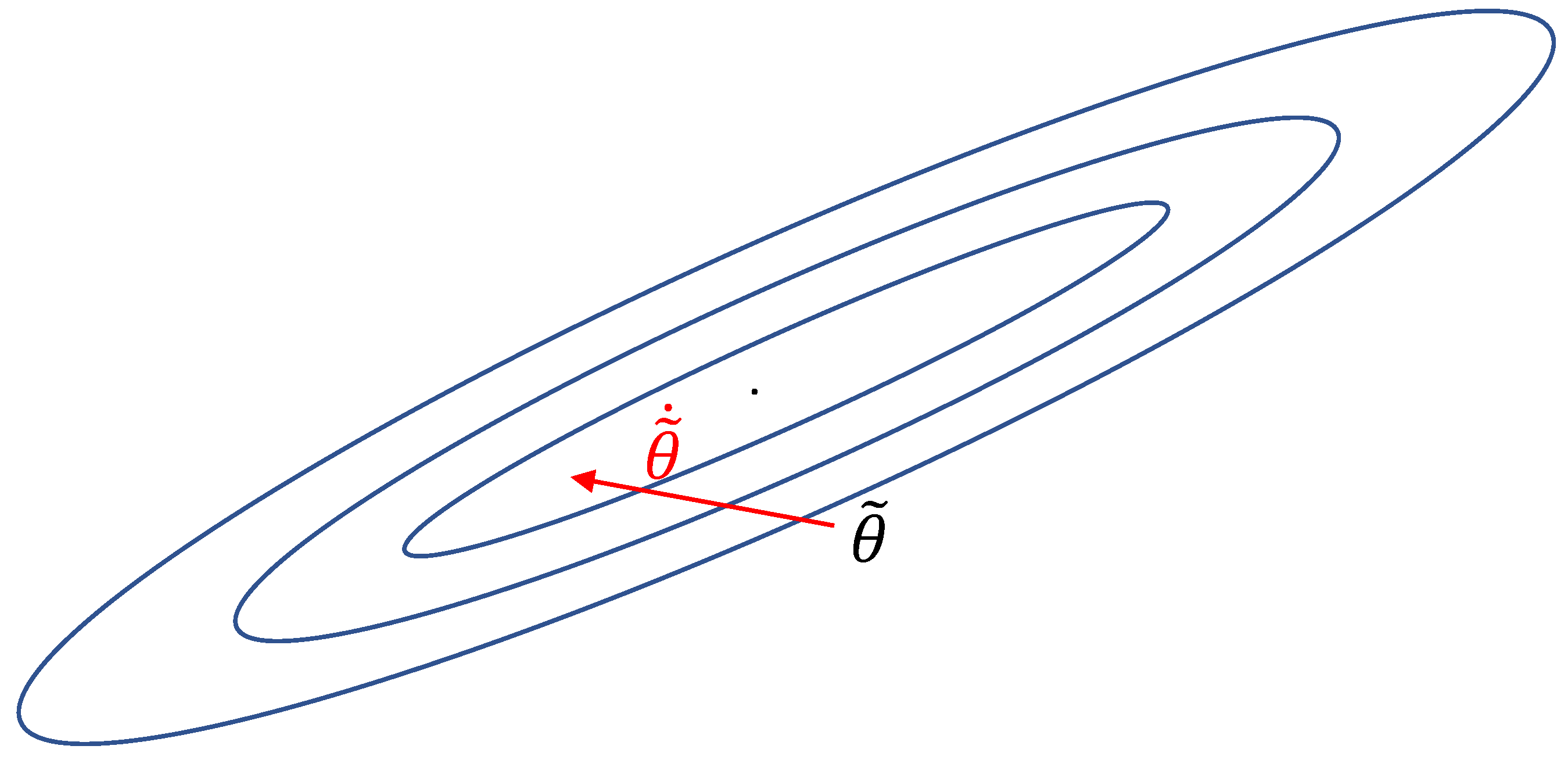
The constraints on parameter $\mu$ in Theorems 1 and 2 limit the amount of momentum that can be applied, thereby limiting the potential advantage gained by using a momentum-based algorithm. In the context of static optimization, Lyapunov-like functions are typically constructed as the sum of two terms; one term representing the norm of the error of the parameter estimate and the other term corresponding to the loss cost function [12]. This generalized structure allows for adjustments to the parameter estimate $\tilde{\theta }$, that may not decrease $\parallel \tilde{\mathcal{V}}\parallel$ or $\parallel \tilde{\theta }\parallel$ but can reduce the loss cost function $L(\tilde{\theta },t)$ as shown in Figure 1.

Figure 1. Visualization of momentum-based learning for an ill-conditioned problem; $\tilde{\theta }$ is updated in a direction that increases $\parallel \tilde{\theta }\parallel$ while still decreasing the loss cost function.

In order to incorporate (10) in our Lyapunov function, we introduce the momentum-based composite gradient algorithm

$$\begin{array}{cc}\hfill \dot{\mathcal{V}}\left(t\right)& =-\Gamma \left(t\right)\varphi \left(t\right)e\left(t\right)-{\displaystyle \frac{\beta }{2}}\Gamma \left(t\right){\mathcal{N}}_{\mathrm{r}}\left(t\right)[R\left(t\right)\theta \left(t\right)+Q\left(t\right)],\mathcal{V}\left(0\right)={\mathcal{V}}_0,t\ge 0,\hfill \end{array}$$

(55)

$$\begin{array}{cc}\hfill \dot{\theta }\left(t\right)& =-\beta [\theta \left(t\right)-\mathcal{V}\left(t\right)]{\mathcal{N}}_{\mathrm{r}}\left(t\right),\theta \left(0\right)={\theta }_0,\hfill \end{array}$$

(56)

$$\begin{array}{cc}\hfill \dot{\Gamma }\left(t\right)& =-\Gamma \left(t\right)[\varphi \left(t\right)\varphi {\left(t\right)}^{\mathrm{T}}-F\left(t\right)]\Gamma \left(t\right),\Gamma \left(0\right)={\Gamma }_0,\hfill \end{array}$$

(57)

where $R(·)$ and $Q(·)$ are given by (12) and (13). Note that this composite update law includes an integral gradient term as well as a recursive least squares term in (55).

Theorem 3. 

Let $\mu >{\displaystyle \frac{2}{\beta }}$, and consider the momentum-based composite gradient algorithm (55)–(57). Then, the following statements hold:

$\left(i\right)$ If there exists ${\alpha }_1>0$ such that (44) holds, then $\theta \in {\mathcal{L}}_{\infty }$, $\dot{\theta },\dot{\mathcal{V}},\mathrm{and}(\theta -\mathcal{V})\in {\mathcal{L}}_{\infty }$, and ${lim}_{t\to \infty }\dot{\theta }\left(t\right)=0$.

$\left(ii\right)$ If $F\left(t\right)=\nu H\left(t\right)$ and $\varphi (·)$ is persistently excited, then the zero solution $(\tilde{\mathcal{V}}\left(t\right),\tilde{\theta }\left(t\right))\equiv (0,0)$ to (55)–(57) is exponentially stable.

Proof. 

This proof is similar to the proof of Theorem 2. Namely, consider the positive-definite function

$$\begin{array}{c}\hfill V(\tilde{\mathcal{V}},\tilde{\theta },t)\triangleq {\tilde{\mathcal{V}}}^{\mathrm{T}}H\left(t\right)\tilde{\mathcal{V}}+{(\tilde{\theta }-\tilde{\mathcal{V}})}^{\mathrm{T}}H\left(t\right)(\tilde{\theta }-\tilde{\mathcal{V}})+2L(\tilde{\theta },t)\end{array}$$

(58)

satisfying $V(0,0,t)=0,t\ge 0$, and note that

$$\begin{array}{cc}\hfill \dot{L}(\tilde{\theta },t)& ={\displaystyle \frac{\partial L}{\partial \tilde{\theta }}}{\displaystyle \frac{\mathrm{d}\tilde{\theta }}{\mathrm{d}\mathrm{t}}}+{\displaystyle \frac{\partial L}{\partial t}}={\tilde{\theta }}^{\mathrm{T}}R\left(t\right)\dot{\tilde{\theta }}-\nu L+{\displaystyle \frac{1}{2}}e{\left(t\right)}^2.\hfill \end{array}$$

(59)

Now, using (49) and (59), note that

$$\begin{array}{cc}\hfill \dot{V}(\tilde{\mathcal{V}},\tilde{\theta },t)& \le -e{\left(t\right)}^2-\parallel F^{{\displaystyle \frac{1}{2}}}{\left(t\right)\mathcal{V}\parallel }^2-{\parallel F^{{\displaystyle \frac{1}{2}}}\left(t\right)(\tilde{\theta }-\tilde{\mathcal{V}})\parallel }^2-\beta {\mathcal{N}}_{\mathrm{r}}\left(t\right){\tilde{\mathcal{V}}}^{\mathrm{T}}R\left(t\right)\tilde{\theta }\hfill \\ \hfill & +\beta {\mathcal{N}}_{\mathrm{r}}\left(t\right){(\tilde{\theta }-\tilde{\mathcal{V}})}^{\mathrm{T}}R\left(t\right)\tilde{\theta }-2{\tilde{\theta }}^{\mathrm{T}}R\left(t\right)\beta (\tilde{\theta }-\tilde{\mathcal{V}}){\mathcal{N}}_{\mathrm{r}}\left(t\right)-2\nu L+e{\left(t\right)}^2\hfill \\ \hfill & \le -\parallel F^{{\displaystyle \frac{1}{2}}}{\left(t\right)\mathcal{V}\parallel }^2-{\parallel F^{{\displaystyle \frac{1}{2}}}\left(t\right)(\tilde{\theta }-\tilde{\mathcal{V}})\parallel }^2-2\beta {\mathcal{N}}_{\mathrm{r}}\left(t\right){\tilde{\theta }}^{\mathrm{T}}R\left(t\right)\tilde{\theta }+2\beta {\mathcal{N}}_{\mathrm{r}}\left(t\right){(\tilde{\theta }-\tilde{\mathcal{V}})}^{\mathrm{T}}R\left(t\right)\tilde{\theta }\hfill \\ \hfill & -2{\tilde{\theta }}^{\mathrm{T}}R\left(t\right)\beta (\tilde{\theta }-\tilde{\mathcal{V}}){\mathcal{N}}_{\mathrm{r}}\left(t\right)-2\nu L\hfill \\ \hfill & \le -\parallel F^{{\displaystyle \frac{1}{2}}}{\left(t\right)\mathcal{V}\parallel }^2-{\parallel F^{{\displaystyle \frac{1}{2}}}\left(t\right)(\tilde{\theta }-\tilde{\mathcal{V}})\parallel }^2-2{\tilde{\theta }}^{\mathrm{T}}R\left(t\right)\tilde{\theta }-2\nu L.\hfill \end{array}$$

(60)

$\left(i\right)$ now follows using similar arguments as in the proof of Theorem 2.

To show $\left(ii\right)$, note that if $\varphi (·)$ is persistently excited, then (44) and (51) hold, and hence, using the fact that $L(\tilde{\theta },t)\le {\displaystyle \frac{1}{\nu }}{\parallel \tilde{\theta }\parallel }^2$, we have

$$\begin{array}{cc}\hfill \left({\displaystyle \frac{3-\sqrt{5}}{2}}\right)e^{-\nu \delta }\rho (\parallel \tilde{\mathcal{V}}{\parallel }^2+\parallel \tilde{\theta }{\parallel }^2)\le V(\tilde{\mathcal{V}},\tilde{\theta },t)& \le \left({\displaystyle \frac{3+\sqrt{5}}{2}}\right){\displaystyle \frac{1}{\nu }}(\parallel \tilde{\mathcal{V}}{\parallel }^2+\parallel \tilde{\theta }{\parallel }^2)+{\displaystyle \frac{1}{\nu }}{\parallel \tilde{\theta }\parallel }^2\hfill \\ & \le \left({\displaystyle \frac{5+\sqrt{5}}{2\nu }}\right)(\parallel \tilde{\mathcal{V}}{\parallel }^2+\parallel \tilde{\theta }{\parallel }^2).\hfill \end{array}$$

(61)

Now, using (49) and (60), it follows that the zero solution $(\tilde{\mathcal{V}}\left(t\right),\tilde{\theta }\left(t\right))\equiv (0,0)$ to (55) and (56) is exponentially stable [15] ([Theorem 4.6]). □

3. System Parameter Identification

In this section, we address the problem of parameter identification using the first- and higher-order tuner algorithms developed in Section 2. First, the following definition is needed.

Definition 2 

([2]). A signal $u:[0,\infty )\to \mathbb{R}$ is stationary and sufficiently rich of order n if the following statements hold:

$\left(i\right)$ The limit

$$\begin{array}{c}\hfill \underset{T\to \infty }{lim}{\displaystyle \frac{1}{T}}{\int }_{t_0}^{t_0+T}u\left(\tau \right)u^{\mathrm{T}}(t+\tau )\mathrm{d}\tau \end{array}$$

(62)

exists uniformly in $t_0$.

$\left(ii\right)$ The support of the spectral measure $S_u\left(\omega \right),\omega \in \mathbb{R}$, of u contains at least n points.

Consider the stable single-input, single-output (SISO) plant, with output $y(·)$ and input $u(·)$ being the only available signals for measurement, given by

$$\begin{array}{cc}\hfill \dot{x}\left(t\right)& =Ax\left(t\right)+Bu\left(t\right),x\left(0\right)=x_0,t\ge 0,\hfill \end{array}$$

(63)

$$\begin{array}{cc}\hfill y\left(t\right)& =C^{\mathrm{T}}x\left(t\right),\hfill \end{array}$$

(64)

where $x\left(t\right)\in {\mathbb{R}}^n,t\ge 0$, $A\in {\mathbb{R}}^{n\times n}$, and $B,C\in {\mathbb{R}}^n$. Since there are an infinite number of triples ($A,B,C$) yielding the same input–output measurements, we cannot uniquely define the $n^2+2n$ coefficients in ($A,B,C$). However, we can determine the $n+m+1$ parameters corresponding to the coefficients of the stable and strictly proper rational transfer function $G\in \mathbb{R}\left(s\right)$ given by

$$\begin{array}{c}\hfill G\left(s\right)=C^{\mathrm{T}}{(s{I}_n-A)}^{-1}B={\displaystyle \frac{\widehat{y}\left(s\right)}{\widehat{u}\left(s\right)}}={\displaystyle \frac{b_m{s}^m+b_{m-1}{s}^{m-1}+\cdots +b_0}{s^n+a_{n-1}{s}^{n-1}+\cdots +a_0}},\end{array}$$

(65)

where, for $s\in \mathbb{C}$, $\widehat{y}\left(s\right)$ is the system output, $\widehat{u}\left(s\right)$ is the system input, and the coefficients $a_i$, $i=0,\cdots ,n-1$, and $b_j$, $j=0,\cdots ,m$, where $m\le n-1$, are unknown system parameters. The goal of the system parameter identification problem is to identify the system parameter vector

$$\begin{array}{c}\hfill {\theta }^{*}=[b_m,b_{m-1},\cdots ,b_0,a_{n-1},\cdots ,a_0]\end{array}$$

(66)

containing the unknown coefficients of the plant transfer function that satisfies

$$\begin{array}{c}\hfill s^n\widehat{y}\left(s\right)={\theta }^{*\mathrm{T}}\widehat{Y}\left(s\right),\end{array}$$

(67)

where $\widehat{Y}\left(s\right)\triangleq {[{\alpha }_m^{\mathrm{T}}\left(s\right)\widehat{u}\left(s\right),-{\alpha }_{n-1}^{\mathrm{T}}\left(s\right)\widehat{y}\left(s\right)]}^{\mathrm{T}}$ and ${\alpha }_i\left(s\right)\triangleq {[s^i,s^{i-1},\cdots ,1]}^{\mathrm{T}}$.

Note that (67) has the form of (1) in the frequency domain; however, in most applications the only signals that are available for measurement are the input $u\left(t\right),t\ge 0$, and the output $y\left(t\right),t\ge 0$, and not their derivatives. To address this, we filter (67) through a stable filter ${\displaystyle \frac{1}{\Lambda \left(s\right)}}$, where $\Lambda \left(s\right)$ is an arbitrary monic Hurwitz polynomial of degree n, to obtain, for $y\left(0\right)=0$,

$$\begin{array}{c}\hfill \widehat{z}\left(s\right)={\theta }^{*\mathrm{T}}\widehat{\varphi }\left(s\right),\end{array}$$

(68)

where $\widehat{z}\left(s\right)\triangleq {\displaystyle \frac{s^n\widehat{y}\left(s\right)}{\Lambda \left(s\right)}}$ and $\widehat{\varphi }\left(s\right)\triangleq {[{\displaystyle \frac{{\alpha }_m^{\mathrm{T}}\left(s\right)}{\Lambda \left(s\right)}}\widehat{u}\left(s\right),-{\displaystyle \frac{{\alpha }_{n-1}^{\mathrm{T}}\left(s\right)}{\Lambda \left(s\right)}}\widehat{y}\left(s\right)]}^{\mathrm{T}}$. The time signals $\varphi \left(t\right),t\ge 0$, and $z\left(t\right),t\ge 0$, can be generated by the state equations ([2])

$$\begin{array}{cc}\hfill {\dot{\varphi }}_0\left(t\right)& ={\Lambda }_{\mathrm{c}}{\varphi }_0\left(t\right)+b_{\mathrm{c}}u\left(t\right),{\varphi }_0\left(0\right)=0,t\ge 0,\hfill \end{array}$$

(69)

$$\begin{array}{cc}\hfill {\varphi }_1\left(t\right)& =P_0{\varphi }_0\left(t\right),\hfill \end{array}$$

(70)

$$\begin{array}{cc}\hfill {\dot{\varphi }}_2\left(t\right)& ={\Lambda }_{\mathrm{c}}{\varphi }_2\left(t\right)-b_{\mathrm{c}}y\left(t\right),{\varphi }_2\left(0\right)=0,\hfill \end{array}$$

(71)

$$\begin{array}{cc}\hfill \varphi \left(t\right)& ={[{\varphi }_1^{\mathrm{T}}\left(t\right),{\varphi }_2^{\mathrm{T}}\left(t\right)]}^{\mathrm{T}},\hfill \end{array}$$

(72)

$$\begin{array}{cc}\hfill z\left(t\right)& =y\left(t\right)+{\lambda }^{\mathrm{T}}{\varphi }_2\left(t\right),\hfill \end{array}$$

(73)

where, for $t\ge 0$, ${\varphi }_0\left(t\right)\in {\mathbb{R}}^n$, ${\varphi }_1\left(t\right)\in {\mathbb{R}}^{m+1}$, ${\varphi }_2\left(t\right)\in {\mathbb{R}}^n$, and

$$\begin{array}{c}\hfill {\Lambda }_{\mathrm{c}}=\left[\begin{array}{c}-{\lambda }^{\mathrm{T}}\\ I_{n-1}|0_{(n-1)\times 1}\end{array}\right],b_{\mathrm{c}}={[1,0,\cdots ,0]}^{\mathrm{T}},\end{array}$$

(74)

$$\begin{array}{c}\hfill P_0=[0_{(m+1)\times (n-m-1)}|I_{m+1}]\in {\mathbb{R}}^{(m+1)\times n},\lambda ={[{\lambda }_{n-1},{\lambda }_{n-2},\cdots ,{\lambda }_0]}^{\mathrm{T}},\end{array}$$

(75)

and where $\det (s{I}_n-{\Lambda }_{\mathrm{c}})=\Lambda \left(s\right)=s^n+{\lambda }^{\mathrm{T}}{\alpha }_{n-1}\left(s\right)$.

Theorem 4. 

Assume that $G\in \mathbb{R}\left(s\right)$ given by (65) has no pole-zero cancellations and $y\left(0\right)=0$. If u is stationary and sufficiently rich of order $n+m+1$, then the adaptive laws (20)–(23), (36)–(38), and (55)–(57) guarantee that $\theta \left(t\right)$ converges to ${\theta }^{*}$ as $t\to \infty$.

Proof. 

The proof follows from Theorems 1, 2, and 3 by noting that if $u(·)$ is stationary and sufficiently rich of order $n+m+1$ and G has no pole-zero cancellations, then $\varphi (·)$ is PE [2] ([Thm. 5.2.4]). □

Remark 4. 

Note that if $y\left(0\right)\ne 0$, then (68) would involve an additional bias error term. As shown in [2], this term converges to the origin exponentially fast, and hence, Theorem 4 remains valid.

4. Momentum-Based Recursive Least Squares and Model Reference Adaptive Control

Recursive least squares type algorithms were first introduced in adaptive control in [16] and extended in [2,17,18]. In this section, we show how the MRLS algorithm proposed in Section 2 can be extended to the problem of model reference adaptive control for systems with relative degree one.

Consider the linear SISO system given by

$${\widehat{y}}_{\mathrm{p}}\left(s\right)=G\left(s\right){\widehat{u}}_{\mathrm{p}}\left(s\right),$$

(76)

where $G\left(s\right)=k_{\mathrm{p}}{\displaystyle \frac{N_{\mathrm{p}}\left(s\right)}{D_{\mathrm{p}}\left(s\right)}}\in \mathbb{R}\left(s\right)$, $N_{\mathrm{p}}\left(s\right),D_{\mathrm{p}}\left(s\right)\in \mathbb{R}\left[s\right]$ are unknown polynomials, $k_{\mathrm{p}}$ is an unknown constant, ${\widehat{u}}_{\mathrm{p}}\left(s\right)$ is the control system input, and ${\widehat{y}}_{\mathrm{p}}\left(s\right)$ is the system output. As in [18], we make the following assumptions.

$\left(i\right)$$G\in \mathbb{R}\left(s\right)$ is minimum phase and has relative degree one.

$\left(ii\right)$ The degree of $D_{\mathrm{p}}\left(s\right)$ is n.

$\left(iii\right)$ The sign of $k_{\mathrm{p}}$ is known.

The control objective is to design an appropriate control law $u_{\mathrm{p}}\left(t\right),t\ge 0$, such that all the signals of the closed-loop system are bounded and $y_{\mathrm{p}}\left(t\right),t\ge 0$, tracks the output $y_{\mathrm{r}}\left(t\right),t\ge 0$, of a reference model given by

$$\begin{array}{c}\hfill {\widehat{y}}_{\mathrm{r}}\left(s\right)=M\left(s\right)\widehat{r}\left(s\right),\end{array}$$

(77)

where $M\left(s\right)\triangleq {\displaystyle \frac{k_{\mathrm{r}}}{s+a_{\mathrm{r}}}}\in \mathbb{R}\left(s\right)$, $a_{\mathrm{r}}>0$ and $k_{\mathrm{r}}$ are known constants, and $\widehat{r}\left(s\right)$ is the Laplace transform of a bounded piecewise continuous signal $r\left(t\right),t\ge 0$.

To address this problem, consider the filter system ([2])

$$\begin{array}{cc}\hfill {\dot{v}}_1\left(t\right)& =F_{\mathrm{c}}{v}_1\left(t\right)+g_{\mathrm{c}}{u}_{\mathrm{p}}\left(t\right),v_1\left(0\right)=v_{10},t\ge 0,\hfill \end{array}$$

(78)

$$\begin{array}{cc}\hfill {\dot{v}}_2\left(t\right)& =F_{\mathrm{c}}{v}_2\left(t\right)+g_{\mathrm{c}}{y}_{\mathrm{p}}\left(t\right),v_2\left(0\right)=v_{20},\hfill \end{array}$$

(79)

where, for $t\ge 0$, $v_1\left(t\right)\in {\mathbb{R}}^{n-1}$, $v_2\left(t\right)\in {\mathbb{R}}^{n-1}$,

$$\begin{array}{c}\hfill F_{\mathrm{c}}=\left[\begin{array}{c}-{\widehat{\lambda }}^{\mathrm{T}}\\ I_{n-2}|0_{(n-2)\times 1}\end{array}\right]\in {\mathbb{R}}^{(n-1)\times (n-1)},\widehat{\lambda }={[{\lambda }_{n-2},{\lambda }_{n-3},\cdots ,{\lambda }_0]}^{\mathrm{T}},\end{array}$$

(80)

$g_{\mathrm{c}}={[1,0\cdots ,0]}^{\mathrm{T}}\in {\mathbb{R}}^{n-1}$, and $\det (s{I}_{n-1}-F_{\mathrm{c}})=s^{n-1}+{\widehat{\lambda }}^{\mathrm{T}}{\alpha }_{n-2}\left(s\right)=F\left(s\right)$, where $F\left(s\right)\in \mathbb{R}\left[s\right]$ is an arbitrary monic Hurwitz polynomial of degree $n-1$. Here, we use $v_1\left(t\right),t\ge 0$, and $v_2\left(t\right),t\ge 0$, to form the regressor vector

$$\begin{array}{c}\hfill \varphi \left(t\right)={[v_1^{\mathrm{T}}\left(t\right),v_2^{\mathrm{T}}\left(t\right),y_{\mathrm{p}}\left(t\right),r\left(t\right)]}^{\mathrm{T}}\in {\mathbb{R}}^{2n}.\end{array}$$

(81)

Note that the existence of a constant parameter vector ${\theta }^{*}={[{\theta }_1^{*\mathrm{T}},{\theta }_2^{*\mathrm{T}},{\theta }_3^{*},{\theta }_4^{*}]}^{\mathrm{T}}\in {\mathbb{R}}^{2n}$ such that the transfer function of the SISO system (76) with ${\widehat{u}}_{\mathrm{p}}\left(s\right)={\theta }^{*\mathrm{T}}\widehat{\varphi }\left(s\right),$ where $\widehat{\varphi }\left(s\right)=[{\displaystyle \frac{{\alpha }_{n-2}\left(s\right)}{F\left(s\right)}}{\widehat{u}}_{\mathrm{p}}\left(s\right)$, ${\displaystyle \frac{{\alpha }_{n-2}\left(s\right)}{F\left(s\right)}}{\widehat{y}}_{\mathrm{p}}\left(s\right),{\widehat{y}}_{\mathrm{p}}\left(s\right),\widehat{r}\left(s\right)]$, matching the reference model transfer function $M\left(s\right)\in \mathbb{R}\left(s\right)$ is guaranteed by the choice of $M\left(s\right)$ and Assumptions $\left(i\right)$–$\left(iii\right)$.

Next, consider the control law

$$\begin{array}{cc}\hfill {\widehat{u}}_{\mathrm{p}}\left(s\right)& =L\left(s\right){\widehat{\theta }}^{\mathrm{T}}\left(s\right)\widehat{\xi }\left(s\right),\hfill \end{array}$$

(82)

where $\widehat{\theta }\left(s\right)\in {\mathbb{C}}^{2n}$, $L\left(s\right)\triangleq s+{\lambda }_1,{\lambda }_1>0$, and $\widehat{\xi }\left(s\right)\triangleq L^{-1}\left(s\right)\widehat{\varphi }\left(s\right)\in {\mathbb{C}}^{2n}$, and note that the tracking error ${\widehat{e}}_1\left(s\right)\triangleq {\widehat{y}}_{\mathrm{p}}\left(s\right)-{\widehat{y}}_{\mathrm{r}}\left(s\right)$ satisfies

$$\begin{array}{c}\hfill {\widehat{e}}_1\left(s\right)=M\left(s\right)L\left(s\right)k^{*}[{\widehat{u}}_{\mathrm{p}}\left(s\right)-{\theta }^{*\mathrm{T}}\widehat{\varphi }\left(s\right)]=M\left(s\right)L\left(s\right)k^{*}{\widehat{\tilde{\theta }}}^{\mathrm{T}}\left(s\right)\widehat{\xi }\left(s\right),\end{array}$$

(83)

where $k^{*}={\displaystyle \frac{k_{\mathrm{p}}}{k_{\mathrm{r}}}}$. Note that (83) has a nonminimal state-space realization given by

$$\begin{array}{cc}\hfill {\dot{e}}_2\left(t\right)& =A_m{e}_2\left(t\right)+B_m{k}^{*}{\tilde{\theta }}^{\mathrm{T}}\left(t\right)\xi \left(t\right),e_2\left(0\right)=e_{20},t\ge 0,\hfill \end{array}$$

(84)

$$\begin{array}{cc}\hfill e_1\left(t\right)& =C_{m}e\left(t\right)+k_{\mathrm{r}}{k}^{*}{\tilde{\theta }}^{\mathrm{T}}\left(t\right)\xi \left(t\right),\hfill \end{array}$$

(85)

where $e_2\left(t\right)\in {\mathbb{R}}^{3n-2}$, $A_m\in {\mathbb{R}}^{(3n-2)\times (3n-2)}$, $B_m={\mathbb{R}}^{(3n-2)\times 1}$, and $C_m={\mathbb{R}}^{1\times (3n-2)}$. Furthermore, note that

$$\begin{array}{c}\hfill M\left(s\right)L\left(s\right)={\displaystyle \frac{k_{\mathrm{r}}(s+{\lambda }_1)}{s+a_{\mathrm{r}}}}={\displaystyle \frac{k_{\mathrm{r}}({\lambda }_1-a_{\mathrm{r}})}{s+a_{\mathrm{r}}}}+k_{\mathrm{r}},\end{array}$$

(86)

where ${\lambda }_1>a_{\mathrm{r}}$, ${\displaystyle \frac{k_{\mathrm{r}}({\lambda }_1-a_{\mathrm{r}})}{s+a_{\mathrm{r}}}}$ is a strictly positive real transfer function. In this case, it follows from the Meyer–Kalman–Popov lemma [2] ([Lem. 3.5.4]) that there exist $(3n-2)\times (3n-2)$ positive-definite matrices $P>0$ and $Q>0$ such that

$$\begin{array}{cc}\hfill A_m^{\mathrm{T}}P+P{A}_m& =-2Q,\hfill \end{array}$$

(87)

$$\begin{array}{cc}\hfill P{B}_m& =C_m^{\mathrm{T}}.\hfill \end{array}$$

(88)

Since for every nonsingular matrix $S\in {\mathbb{R}}^{(3n-2)\times (3n-2)}$ and constant $\alpha >0$, the realizations $(A,B,C)$ and $(SA{S}^{-1}$, $\alpha SB$, ${\alpha }^{-1}C{S}^{-1}$) are equivalent, choosing $S=Q^{{\displaystyle \frac{1}{2}}}$ and $\alpha =\parallel C_m\parallel$ we can ensure that $(A_m,B_m,C_m)$ is a realization that satisfies (87) and (88) with $Q=I_{3n-2}$ and $C_m$ is normalized so that $\parallel C_m\parallel =1$.

Next, consider the recursive least-squares algorithm given by

$$\begin{array}{cc}\hfill \dot{\theta }\left(t\right)& =-\alpha \mathrm{sgn}\left(k^{*}\right)\Gamma \left(t\right)\xi \left(t\right)e_1\left(t\right),\theta \left(0\right)={\theta }_0,t\ge 0,\hfill \end{array}$$

(89)

$$\begin{array}{cc}\hfill \dot{\Gamma }\left(t\right)& =\nu \Gamma \left(t\right)-\Gamma \left(t\right)\xi \left(t\right)\xi {\left(t\right)}^{\mathrm{T}}\Gamma \left(t\right),\Gamma \left(0\right)={\Gamma }_0,\hfill \end{array}$$

(90)

where $\mathrm{sgn}\left(\sigma \right)\triangleq \sigma /|\sigma |,\sigma \ne 0,$ and $\mathrm{sgn}\left(0\right)\triangleq 0$, $\alpha >0$, and $\nu \ge 0$. Note that for $\nu =0$, (89) and (90) recover the recursive least-squares algorithm of [19].

Here, we modify the recursive least-squares algorithm (89) and (90) to construct our MRLS algorithm as

$$\begin{array}{cc}\hfill \dot{\mathcal{V}}\left(t\right)& =-\gamma \mathrm{sgn}\left(k^{*}\right)\Gamma \left(t\right)\xi \left(t\right)e_1\left(t\right),\mathcal{V}\left(0\right)={\mathcal{V}}_0,t\ge 0,\hfill \end{array}$$

(91)

$$\begin{array}{cc}\hfill \dot{\theta }\left(t\right)& =-\beta (\theta \left(t\right)-\mathcal{V}\left(t\right)){\mathcal{N}}_{\mathrm{m}}\left(t\right),\theta \left(0\right)={\theta }_0,\hfill \end{array}$$

(92)

$$\begin{array}{cc}\hfill \dot{\Gamma }\left(t\right)& =\nu \Gamma \left(t\right)-\Gamma \left(t\right)\xi \left(t\right)\xi {\left(t\right)}^{\mathrm{T}}\Gamma \left(t\right),\Gamma \left(0\right)={\Gamma }_0,\hfill \end{array}$$

(93)

where $\beta >0$, $\gamma >0$, $\alpha >0$, $\nu >0$,

$$\begin{array}{c}\hfill {\mathcal{N}}_{\mathrm{m}}\left(t\right)\triangleq 1+\mu \xi {\left(t\right)}^{\mathrm{T}}\Gamma \left(t\right)\xi \left(t\right)=1+\mu {\parallel {\Gamma }^{{\displaystyle \frac{1}{2}}}\left(t\right)\xi \left(t\right)\parallel }^2,\end{array}$$

(94)

and $\mu >0$. Note that (91) and (92) can be rewritten in terms of the error parameters $\tilde{\mathcal{V}}\left(t\right),t\ge 0$, and $\tilde{\theta }\left(t\right),t\ge 0,$ as

$$\begin{array}{cc}\hfill \dot{\tilde{\mathcal{V}}}\left(t\right)& =-\gamma \mathrm{sgn}\left(k^{*}\right)\Gamma \left(t\right)\xi \left(t\right)e_1\left(t\right),\tilde{\mathcal{V}}\left(0\right)={\mathcal{V}}_0-{\mathcal{V}}^{*},t\ge 0,\hfill \end{array}$$

(95)

$$\begin{array}{cc}\hfill \dot{\tilde{\theta }}\left(t\right)& =-\beta (\tilde{\theta }\left(t\right)-\tilde{\mathcal{V}}\left(t\right)){\mathcal{N}}_{\mathrm{m}}\left(t\right),\tilde{\theta }\left(0\right)={\theta }_0-{\theta }^{*}.\hfill \end{array}$$

(96)

Theorem 5. 

Consider the SISO system (76) with control law (82) and the MRLS algorithm given by (91)–(93) with $\alpha >{\displaystyle \frac{1}{|k_{\mathrm{r}}||k^{*}|}}$ and $\mu >{\displaystyle \frac{1}{\beta }}(1+{\displaystyle \frac{2\alpha |k^{*}|}{\zeta }})$, where $\zeta \le min\{1,{\displaystyle \frac{1}{2k_{\mathrm{r}}}}\}$. Then $e_2\in {\mathcal{L}}_2\cap {\mathcal{L}}_{\infty }$ and ${\tilde{\theta }}^{\mathrm{T}}\xi \in {\mathcal{L}}_2$. If, in addition, $\nu =0$, then $\tilde{\theta },\tilde{\mathcal{V}}\in {\mathcal{L}}_{\infty }$ and ${lim}_{t\to \infty }{e}_1\left(t\right)=0$.

Proof. 

Consider the function

$$\begin{array}{c}\hfill V(\tilde{\theta },\tilde{\mathcal{V}},e_2,t)\triangleq {\alpha }^{-1}|k^{*}|{\tilde{\mathcal{V}}}^{\mathrm{T}}H\left(t\right)\tilde{\mathcal{V}}+{\alpha }^{-1}|k^{*}|{(\tilde{\theta }-\tilde{\mathcal{V}})}^{\mathrm{T}}H\left(t\right)(\tilde{\theta }-\tilde{\mathcal{V}})+e_2^{\mathrm{T}}P{e}_2,\end{array}$$

where $P>0$ satisfies (87) and (88), and note that

$$\begin{array}{cc}\hfill \dot{V}& (\tilde{\theta },\tilde{\mathcal{V}},e_2,t)\hfill \\ \hfill & =e_2^{\mathrm{T}}P{\dot{e}}_2+2|k^{*}|{\alpha }^{-1}{\tilde{\mathcal{V}}}^{\mathrm{T}}H\left(t\right)\dot{\tilde{\mathcal{V}}}+|k^{*}|{\alpha }^{-1}{\tilde{\mathcal{V}}}^{\mathrm{T}}\dot{H}\left(t\right)\tilde{\mathcal{V}}+|k^{*}|{\alpha }^{-1}{(\tilde{\theta }-\tilde{\mathcal{V}})}^{\mathrm{T}}\dot{H}\left(t\right)(\tilde{\theta }-\tilde{\mathcal{V}})\hfill \\ \hfill & +2|k^{*}|{\alpha }^{-1}{(\tilde{\theta }-\tilde{\mathcal{V}})}^{\mathrm{T}}H\left(t\right)(\dot{\tilde{\theta }}-\dot{\tilde{\mathcal{V}}})\hfill \\ \hfill & =-2\parallel e_2{\parallel }^2+2e_2^{\mathrm{T}}P{B}_m{k}^{*}{\tilde{\theta }}^{\mathrm{T}}\xi \left(t\right)-2k^{*}{\tilde{\mathcal{V}}}^{\mathrm{T}}\xi \left(t\right)e_1+|k^{*}|{\alpha }^{-1}{\tilde{\mathcal{V}}}^{\mathrm{T}}\dot{H}\left(t\right)\tilde{\mathcal{V}}\hfill \\ \hfill & +|k^{*}|{\alpha }^{-1}{(\tilde{\theta }-\tilde{\mathcal{V}})}^{\mathrm{T}}\dot{H}\left(t\right)(\tilde{\theta }-\tilde{\mathcal{V}})-2\beta |k^{*}|{\alpha }^{-1}{(\tilde{\theta }-\tilde{\mathcal{V}})}^{\mathrm{T}}H\left(t\right)(\tilde{\theta }-\tilde{\mathcal{V}}){\mathcal{N}}_{\mathrm{m}}\left(t\right)\hfill \\ \hfill & +2k^{*}{(\tilde{\theta }-\tilde{\mathcal{V}})}^{\mathrm{T}}\xi \left(t\right)e_1\hfill \\ \hfill & =-2\parallel e_2{\parallel }^2+2{\left(C_m{e}_2\right)}^{\mathrm{T}}{k}^{*}{\tilde{\theta }}^{\mathrm{T}}\xi \left(t\right)-2k^{*}{\tilde{\mathcal{V}}}^{\mathrm{T}}\xi \left(t\right)e_1+|k^{*}|{\alpha }^{-1}{\tilde{\mathcal{V}}}^{\mathrm{T}}\dot{H}\left(t\right)\tilde{\mathcal{V}}\hfill \\ \hfill & +|k^{*}|{\alpha }^{-1}{(\tilde{\theta }-\tilde{\mathcal{V}})}^{\mathrm{T}}\dot{H}\left(t\right)(\tilde{\theta }-\tilde{\mathcal{V}})-2\beta |k^{*}|{\alpha }^{-1}{(\tilde{\theta }-\tilde{\mathcal{V}})}^{\mathrm{T}}H\left(t\right)(\tilde{\theta }-\tilde{\mathcal{V}}){\mathcal{N}}_{\mathrm{m}}\left(t\right)\hfill \\ \hfill & +2k^{*}{(\tilde{\theta }-\tilde{\mathcal{V}})}^{\mathrm{T}}\xi \left(t\right)e_1\hfill \\ \hfill & =-2\parallel e_2{\parallel }^2+2{(e_1-k_{\mathrm{r}}{k}^{*}{\tilde{\theta }}^{\mathrm{T}}\xi \left(t\right))}^{\mathrm{T}}{k}^{*}{\tilde{\theta }}^{\mathrm{T}}\xi \left(t\right)-2k^{*}{\tilde{\mathcal{V}}}^{\mathrm{T}}\xi \left(t\right)e_1\hfill \\ \hfill & +|k^{*}|{\alpha }^{-1}{\tilde{\mathcal{V}}}^{\mathrm{T}}[-F\left(t\right)+\xi \left(t\right)\xi {\left(t\right)}^{\mathrm{T}}]\tilde{\mathcal{V}}+|k^{*}|{\alpha }^{-1}{(\tilde{\theta }-\tilde{\mathcal{V}})}^{\mathrm{T}}[-F\left(t\right)+\hfill \\ \hfill & \xi \left(t\right)\xi {\left(t\right)}^{\mathrm{T}}](\tilde{\theta }-\tilde{\mathcal{V}})-2\beta |k^{*}|{\alpha }^{-1}{(\tilde{\theta }-\tilde{\mathcal{V}})}^{\mathrm{T}}H\left(t\right)(\tilde{\theta }-\tilde{\mathcal{V}}){\mathcal{N}}_{\mathrm{m}}\left(t\right)+2k^{*}{(\tilde{\theta }-\tilde{\mathcal{V}})}^{\mathrm{T}}\xi \left(t\right)e_1\hfill \\ \hfill & =-2\parallel e_2{\parallel }^2-|k^{*}|{\alpha }^{-1}\parallel F^{{\displaystyle \frac{1}{2}}}{\left(t\right)\mathcal{V}\parallel }^2-|k^{*}|{\alpha }^{-1}{\parallel F^{{\displaystyle \frac{1}{2}}}\left(t\right)(\tilde{\theta }-\tilde{\mathcal{V}})\parallel }^2-2k_{\mathrm{r}}{\left(k^{*}{\tilde{\theta }}^{\mathrm{T}}\xi \left(t\right)\right)}^2\hfill \\ \hfill & +4e_1{k}^{*}{(\tilde{\theta }-\tilde{\mathcal{V}})}^{\mathrm{T}}\xi \left(t\right)+|k^{*}|{\alpha }^{-1}|{\tilde{\mathcal{V}}}^{\mathrm{T}}\xi \left(t\right){|}^2+|k^{*}|{\alpha }^{-1}{|{(\tilde{\theta }-\tilde{\mathcal{V}})}^{\mathrm{T}}\xi \left(t\right)|}^2\hfill \\ \hfill & -2\beta |k^{*}|{\alpha }^{-1}{\parallel {(\tilde{\theta }-\tilde{\mathcal{V}})}^{\mathrm{T}}{H}^{{\displaystyle \frac{1}{2}}}\left(t\right)\parallel }^2{\mathcal{N}}_{\mathrm{m}}\left(t\right),t\ge 0.\hfill \end{array}$$

(97)

Next, using the Cauchy–Schwarz and Young inequalities we obtain

$$\begin{array}{cc}\hfill e_1^2& =e_2^{\mathrm{T}}{C}_m^{\mathrm{T}}{C}_m{e}_2+{\left(k_{\mathrm{r}}{k}^{*}{\tilde{\theta }}^{\mathrm{T}}\xi \left(t\right)\right)}^2+2k_{\mathrm{r}}{k}^{*}{\tilde{\theta }}^{\mathrm{T}}{e}_2^{\mathrm{T}}{C}_m\hfill \\ \hfill & \le \parallel C_m{\parallel }^2\parallel e_2{\parallel }^2+{\left(k_{\mathrm{r}}{k}^{*}{\tilde{\theta }}^{\mathrm{T}}\xi \left(t\right)\right)}^2+2k_{\mathrm{r}}\parallel k^{*}{\tilde{\theta }}^{\mathrm{T}}\xi \left(t\right)\parallel \parallel e_2^{\mathrm{T}}{C}_m\parallel \hfill \\ \hfill & \le 2\parallel C_m{\parallel }^2{\parallel e_2\parallel }^2+2{\left(k_{\mathrm{r}}{k}^{*}{\tilde{\theta }}^{\mathrm{T}}\xi \left(t\right)\right)}^2\hfill \\ \hfill & \le 2\parallel e_2{\parallel }^2+2{\left(k_{\mathrm{r}}{k}^{*}{\tilde{\theta }}^{\mathrm{T}}\xi \left(t\right)\right)}^2.\hfill \end{array}$$

(98)

Now, using (98) along with triangle inequality $|{\tilde{\mathcal{V}}}^{\mathrm{T}}{\xi \left(t\right)|}^2\le |{\tilde{\theta }}^{\mathrm{T}}{\xi \left(t\right)|}^2+{|{(\tilde{\theta }-\tilde{\mathcal{V}})}^{\mathrm{T}}\xi \left(t\right)|}^2$, $t\ge 0$, it follows from (97) that

$$\begin{array}{cc}\hfill \dot{V}& (\tilde{\theta },\tilde{\mathcal{V}},e_2,t)\hfill \\ \hfill & \le -2(1-\zeta )\parallel e_2{\parallel }^2-\zeta e_1^2+2\zeta {\left(k_{\mathrm{r}}{k}^{*}{\tilde{\theta }}^{\mathrm{T}}\xi \left(t\right)\right)}^2-|k^{*}|{\alpha }^{-1}{\parallel F^{{\displaystyle \frac{1}{2}}}\left(t\right)\mathcal{V}\parallel }^2-2k_{\mathrm{r}}{\left(k^{*}{\tilde{\theta }}^{\mathrm{T}}\xi \left(t\right)\right)}^2\hfill \\ \hfill & -|k^{*}|{\alpha }^{-1}\parallel F^{{\displaystyle \frac{1}{2}}}\left(t\right)(\tilde{\theta }-\tilde{\mathcal{V}}){\parallel }^2+4|e_1||k^{*}|{(\tilde{\theta }-\tilde{\mathcal{V}})}^{\mathrm{T}}\xi \left(t\right)+|k^{*}|{\alpha }^{-1}[|{\tilde{\theta }}^{\mathrm{T}}\xi \left(t\right){|}^2\hfill \\ \hfill & +\parallel {(\tilde{\theta }-\tilde{\mathcal{V}})}^{\mathrm{T}}\xi \left(t\right){\parallel }^2]+|k^{*}|{\alpha }^{-1}{|{(\tilde{\theta }-\tilde{\mathcal{V}})}^{\mathrm{T}}\xi \left(t\right)|}^2\hfill \\ \hfill & -2\beta |k^{*}|{\alpha }^{-1}{\parallel {(\tilde{\theta }-\tilde{\mathcal{V}})}^{\mathrm{T}}{H}^{{\displaystyle \frac{1}{2}}}\left(t\right)\parallel }^2{\mathcal{N}}_{\mathrm{m}}\left(t\right)\hfill \\ \hfill & \le -2(1-\zeta )\parallel e_2{\parallel }^2+|k^{*}|(-2k_{\mathrm{r}}|k^{*}|+2\zeta k_{\mathrm{r}}^2|k^{*}|+{\alpha }^{-1})|{\tilde{\theta }}^{\mathrm{T}}{\xi \left(t\right)|}^2\hfill \\ \hfill & -|k^{*}|{\alpha }^{-1}{\parallel F^{{\displaystyle \frac{1}{2}}}\left(t\right)\mathcal{V}\parallel }^2\hfill \\ \hfill & -[\sqrt{\zeta }|e_1|-2{\displaystyle \frac{|k^{*}|}{\sqrt{\zeta }}}|{(\tilde{\theta }-\tilde{\mathcal{V}})}^{\mathrm{T}}\xi \left(t\right){|]}^2+\left(2|k^{*}|{\alpha }^{-1}+4{\displaystyle \frac{|k^{*}{|}^2}{\zeta }}\right){|{(\tilde{\theta }-\tilde{\mathcal{V}})}^{\mathrm{T}}\xi \left(t\right)|}^2\hfill \\ \hfill & -|k^{*}|{\alpha }^{-1}\parallel F^{{\displaystyle \frac{1}{2}}}\left(t\right)(\tilde{\theta }-\tilde{\mathcal{V}}){\parallel }^2-2\beta |k^{*}|{\alpha }^{-1}{\parallel {(\tilde{\theta }-\tilde{\mathcal{V}})}^{\mathrm{T}}{H}^{{\displaystyle \frac{1}{2}}}\left(t\right)\parallel }^2{\mathcal{N}}_{\mathrm{m}}\left(t\right)\hfill \\ \hfill & \le -2(1-\zeta )\parallel e_2{\parallel }^2+|k^{*}|(-2k_{\mathrm{r}}|k^{*}|+2\zeta k_{\mathrm{r}}^2|k^{*}|+{\alpha }^{-1})|{\tilde{\theta }}^{\mathrm{T}}{\xi \left(t\right)|}^2\hfill \\ \hfill & -|k^{*}|{\alpha }^{-1}{\parallel F^{{\displaystyle \frac{1}{2}}}\left(t\right)\mathcal{V}\parallel }^2\hfill \\ \hfill & +\left(2|k^{*}|{\alpha }^{-1}+{\displaystyle \frac{4|k^{*}{|}^2}{\zeta }}-2\beta \mu |k^{*}|{\alpha }^{-1}\right)|{(\tilde{\theta }-\tilde{\mathcal{V}})}^{\mathrm{T}}{H}^{{\displaystyle \frac{1}{2}}}\left(t\right){|}^2\parallel {\Gamma }^{{\displaystyle \frac{1}{2}}}\left(t\right)\xi \left(t\right)\parallel \hfill \\ \hfill & -|k^{*}|{\alpha }^{-1}\parallel F^{{\displaystyle \frac{1}{2}}}\left(t\right)(\tilde{\theta }-\tilde{\mathcal{V}}){\parallel }^2-2\beta |k^{*}|{\alpha }^{-1}{\parallel {(\tilde{\theta }-\tilde{\mathcal{V}})}^{\mathrm{T}}{H}^{{\displaystyle \frac{1}{2}}}\left(t\right)\parallel }^2\hfill \\ \hfill & \le -2(1-\zeta )\parallel e_2{\parallel }^2+|k^{*}|(-2k_{\mathrm{r}}|k^{*}|+2\zeta k_{\mathrm{r}}^2|k^{*}|+{\alpha }^{-1})|{\tilde{\theta }}^{\mathrm{T}}{\xi \left(t\right)|}^2\hfill \\ \hfill & -|k^{*}|{\alpha }^{-1}\parallel F^{{\displaystyle \frac{1}{2}}}{\left(t\right)\mathcal{V}\parallel }^2-|k^{*}|{\alpha }^{-1}{\parallel F^{{\displaystyle \frac{1}{2}}}\left(t\right)(\tilde{\theta }-\tilde{\mathcal{V}})\parallel }^2\hfill \\ \hfill & -2\beta |k^{*}|{\alpha }^{-1}{\parallel {(\tilde{\theta }-\tilde{\mathcal{V}})}^{\mathrm{T}}{H}^{{\displaystyle \frac{1}{2}}}\left(t\right)\parallel }^2\hfill \\ \hfill & \le 0,t\ge 0,\hfill \end{array}$$

which shows that $V(\tilde{\theta },\tilde{\mathcal{V}},e_2,t)\in {\mathcal{L}}_{\infty }$. Hence, ${\tilde{\mathcal{V}}}^{\mathrm{T}}H\left(t\right)\tilde{\mathcal{V}}$, ${(\tilde{\theta }-\tilde{\mathcal{V}})}^{\mathrm{T}}H\left(t\right)(\tilde{\theta }-\tilde{\mathcal{V}})\in {\mathcal{L}}_{\infty },t\ge 0$, $e_2^{\mathrm{T}}P{e}_2\in {\mathcal{L}}_{\infty }$. Next, integrating $\dot{V}$ over $[0,\infty )$ yields

$$\begin{array}{c}\hfill {\int }_0^{\infty }{\parallel e_2\left(\tau \right)\parallel }^2\mathrm{d}\tau \le V({\tilde{\mathcal{V}}}_0,{\tilde{\theta }}_0,e_{20},0)-\underset{t\to \infty }{lim}V(\tilde{\mathcal{V}}\left(t\right),\tilde{\theta }\left(t\right),e_2\left(t\right),t)<\infty ,\end{array}$$

and hence, $e_2\in {\mathcal{L}}_2$. Similarly, ${\tilde{\theta }}^{\mathrm{T}}\xi \in {\mathcal{L}}_2$ and, since $P>0$, $e_2\in {\mathcal{L}}_{\infty }$.

Finally, if $\nu =0$, then $H\left(t\right)$ satisfies

$$\begin{array}{cc}\hfill \dot{H}\left(t\right)& =\xi \left(t\right)\xi {\left(t\right)}^{\mathrm{T}},H\left(0\right)={\Gamma }_0^{-1},t\ge 0,\hfill \end{array}$$

(99)

or

$$H\left(t\right)={\Gamma }_0^{-1}+{\int }_0^t\xi \left(\tau \right)\xi {\left(\tau \right)}^{\mathrm{T}}\mathrm{d}\tau .$$

(100)

Hence, $H\left(t\right)>{\Gamma }_0^{-1},t\ge 0$, and thus, $\tilde{\mathcal{V}},\tilde{\theta }\in {\mathcal{L}}_{\infty }$. Now, if $e_1,\tilde{\theta }\in {\mathcal{L}}_{\infty }$, then (85) implies that ${\dot{e}}_1\in {\mathcal{L}}_{\infty }$ and, by Lemma 2, ${lim}_{t\to \infty }{e}_1\left(t\right)=0$. □

Remark 5. 

Note that unlike many MRAC schemes (e.g., [20]), (91)–(93) does not necessitate a projection operator to guarantee boundedness of the tracking error. However, unlike [19], wherein only a lower bound is necessary for $|k^{*}|$, we require knowledge of a lower and upper bound for $|k^{*}|$.

Remark 6. 

It is important to note that there exists an alternative MRAC framework in the litterature known as the normalized adaptive laws [2] whose design is not based on the tracking error $e_1(·)$ but rather on a normalized estimation error of a particular parametrization of the plant. For this framework, the momentum-based integral gradient algorithm (20)–(23), the momentum-based recursive least squares algorithms (36)–(38), and momentum-based composite gradient algorithm (55)–(57) can be used directly for strictly proper plants without a relative degree restriction. In this case, the parametrization of the ideal controller is given by $u\left(s\right)={\theta }^{*\mathrm{T}}\varphi \left(s\right)$, where ${\theta }^{*}$ satisfies $\widehat{z}\left(s\right)={\theta }^{*\mathrm{T}}\widehat{\varphi }\left(s\right),$$\widehat{z}\left(s\right)=M\left(s\right)u_{\mathrm{p}}\left(s\right)$, and $\widehat{\varphi }\left(s\right)=[M\left(s\right){\widehat{v}}_1^{\mathrm{T}}\left(s\right),{\widehat{v}}_2^{\mathrm{T}}\left(s\right),M\left(s\right){\widehat{y}}_{\mathrm{p}}\left(s\right),{\widehat{y}}_{\mathrm{p}}\left(s\right)]$.

5. Illustrative Numerical Examples

5.1. System Parameter Identification

Consider the third-order transfer function representing a servo control system for the pitch control of an aircraft given by

$$\begin{array}{c}\hfill \widehat{y}\left(s\right)={\displaystyle \frac{b_{1}s+b_0}{s^3+a_2{s}^2+a_{1}s+a_0}}\widehat{u}\left(s\right),\end{array}$$

(101)

where $\widehat{y}\left(s\right)\in \mathbb{C}$ is the pitch angle, $\widehat{u}\left(s\right)\in \mathbb{C}$ is the system input, and $b_1$, $b_0$, $a_2$, $a_1$, $a_0>0$, and $b_0\ne 0$ are the unknown system plant parameters. Note that, (68) gives $\widehat{z}\left(s\right)={\displaystyle \frac{s^3}{\Lambda \left(s\right)}}\widehat{y}\left(s\right)$ with ${\theta }^{*}={[b_1,b_0,a_2,a_1,a_0]}^{\mathrm{T}}$ and $\widehat{\varphi }\left(s\right)={[{\displaystyle \frac{[s,1]}{\Lambda \left(s\right)}}\widehat{u}\left(s\right),{\displaystyle \frac{-[s^2,s,1]}{\Lambda \left(s\right)}}\widehat{y}\left(s\right)]}^{\mathrm{T}}$.

Let $a_0=0.1774$, $a_1=2.072$, $a_2=0.739$, $b_0=0.1774$, $b_1=1.151$, $u\left(t\right)=U[cos(4t)+cos(2t)+sin(4t)+sin(t\left)\right]$, $U>0$, and choose $\Lambda \left(s\right)={(s+1)}^3$. Note that $u(·)$ is a stationary and sufficiently rich signal of order five, and hence, Theorem 4 guarantees that the estimated system parameters $\theta \left(t\right)$ will converge exponentially to ${\theta }^{*}$ as $t\to \infty$ using both the momentum-based integral gradient algorithm (20)–(23) and the MRLS algorithm (36)–(38).

First, we compare the performance of the RLS algorithm (34) and (35) with the MRLS algorithm (20)–(23). For this comparison, we set $U=10$, $\Gamma \left(0\right)=3000I_5$, $\nu =0.1$, $\beta =0.1$, $\mu ={\displaystyle \frac{2}{\beta }}$, $\theta \left(0\right)={[0,0,0,0,0]}^{\mathrm{T}}$, and $\mathcal{V}\left(0\right)={[0,0,0,0,0]}^{\mathrm{T}}$. Figure 2 shows the system parameter estimate versus time. It can be seen that for both the RLS and the MRLS algorithms the parameter estimate $\theta \left(t\right)$ converges to ${\theta }^{*}$ as expected by Theorem 2. Moreover, as seen in Figure 3 the MRLS algorithm provides faster convergence of the system parameters to the true values as compared to the standard RLS algorithm.

Figure 2. Parameter estimate values $\theta \left(t\right)$ versus time using the RLS and MRLS algorithms. In both cases the parameter estimate values converge to the true values with the MRLS algorithm converging faster.

Figure 3. Norm of the parameter estimate error $\tilde{\theta }\left(t\right)$ versus time using the RLS and MRLS algorithms.

Next, we compare the momentum-based composite gradient algorithm (55)–(57) with the composite gradient algorithm given by

$$\begin{array}{cc}\hfill \dot{\theta }\left(t\right)& =-\Gamma \left(t\right)\varphi \left(t\right)e\left(t\right)-{\displaystyle \frac{\beta }{2}}\Gamma \left(t\right){\mathcal{N}}_{\mathrm{r}}\left(t\right)[R\left(t\right)\theta \left(t\right)+Q\left(t\right)],\theta \left(0\right)={\theta }_0,t\ge 0.\hfill \end{array}$$

(102)

Let $U=1$, $\Gamma \left(0\right)=1000I_5$, $\nu =0.2$, $\beta =0.1$, $\mu ={\displaystyle \frac{2}{\beta }}$, $\theta \left(0\right)={[0,0,0,0,0]}^{\mathrm{T}}$, and $\mathcal{V}\left(0\right)={[0,0,0,0,0]}^{\mathrm{T}}$. Figure 4 shows the system parameter estimates versus time. It can be seen that for both the composite gradient and the momentum-based composite gradient algorithms the parameter estimate $\theta \left(t\right)$ converges to ${\theta }^{*}$ as expected by Theorem 3. However, as seen in Figure 5, our proposed algorithm provides faster convergence of the system parameters to their true values. In particular, the momentum-based composite gradient settles around a value of ${10}^{-3}$ at $t=16$ s as compared to 20 s for the composite gradient. Note that the convergence rate due to the addition of momentum is more pronounced in the case of the composite algorithm as compared to the RLS algorithm.

Figure 4. Parameter estimate values $\theta \left(t\right)$ versus time using the composite gradient and the momentum-based composite gradient algorithm. In both cases the parameter estimate values converge to the true values with the momentum-based integral algorithm converging slightly faster.

Figure 5. Norm of the parameter estimate error $\tilde{\theta }\left(t\right)$ versus time using the composite and the momentum-based composite algorithms.

5.2. Momentum-Based Recursive Least Squares and Model Reference Adaptive Control

Here, we consider the short-term dynamics of the aircraft as an example, as shown in Figure 6, where $\alpha$ is the angle of attack, $\gamma$ is the flight path angle, and $U_e$ is the equilibrium linear axial velocity. The transfer function describing the short-term dynamics of the reduced-order longitudinal state equation of the aircraft with angle of attack output and elevator deflection input $\eta$ is given by [21]

$$\begin{array}{c}\hfill {\displaystyle \frac{\widehat{\alpha }\left(s\right)}{\widehat{\eta }\left(s\right)}}={\displaystyle \frac{k_{\mathrm{p}}(s+b_0)}{s^2+a_{1}s+a_0}},\end{array}$$

(103)

where $k_{\mathrm{p}}={\displaystyle \frac{z_{\eta }}{U_e}}$, $b_0=U_e{\displaystyle \frac{m_{\eta }}{z_{\eta }}}$, $a_1=m_q+z_w$, and $a_0=m_q{z}_w-m_w{U}_e$, and $m_{\eta }$, $m_w$, and $m_q$ are the concise partial derivatives (see [21]) of the pitching moment with respect to the elevator angle $\eta$, the normal velocity w, and the pitch rate q. Moreover, $z_{\eta }$ and $z_w$ denote the concise partial derivatives of the normal force on the aircraft with respect to the elevator angle $\eta$ and the normal velocity w. Here, we set $k_{\mathrm{p}}=-0.1601$, $b_0=71.9844$, $a_1=5.0101$, and $a_0=12.9988$ [21].

Figure 6. Schematic of an aircraft.

The desired system performance is to track the reference output

$$\begin{array}{c}\hfill {\widehat{y}}_{\mathrm{r}}\left(s\right)={\displaystyle \frac{5}{s+0.3}}\widehat{r}\left(s\right),\end{array}$$

(104)

where $\widehat{r}\left(s\right)$ is a reference command signal. Next, we use the filter system (78) and (79) with $F_{\mathrm{c}}=-2$ and $g_{\mathrm{c}}=1$, and the control law (82) whose state space realization is given by

$$\begin{array}{cc}\hfill \dot{\xi }\left(t\right)& =-{\lambda }_1\xi \left(t\right)+\varphi \left(t\right),\xi \left(0\right)=0,t\ge 0,\hfill \end{array}$$

(105)

$$\begin{array}{cc}\hfill u_{\mathrm{p}}\left(t\right)& ={\theta }^{\mathrm{T}}\left(t\right)\varphi \left(t\right)+{\dot{\theta }}^{\mathrm{T}}\left(t\right)\xi \left(t\right),\hfill \end{array}$$

(106)

where $\varphi \left(t\right)={[v_1\left(t\right),v_2\left(t\right),y_{\mathrm{p}}\left(t\right),r\left(t\right)]}^{\mathrm{T}}.$ For our simulations, we select the reference signal to be a square wave with a frequency $2\pi$ and amplitude 1. Furthermore, the system initial conditions are set to $y\left(0\right)=0$, $y_p\left(0\right)=0$, ${\dot{y}}_p\left(0\right)=0$, and $\Gamma \left(0\right)=300I_4$.

Next, we compare the RLS algorithm (89) and (90) with our proposed MRLS algorithm (91)–(93). For this comparison, we set ${\lambda }_1=2$, $\alpha =1$, $\beta =1$, $\mu =5$, $\gamma =1$, $\nu =0.3$, $\theta \left(0\right)={[0,0,0,0]}^{\mathrm{T}}$, and $\mathcal{V}\left(0\right)={[0,0,0,0]}^{\mathrm{T}}$. Note that all the conditions of Theorem 5 are satisfied. Figure 7 shows the system parameters versus time for the MRLS and the RLS algorithms. It can be seen that in both cases the system parameters converge to the true values with the MRLS providing faster convergence as compared to the standard RLS update law. Finally, Figure 8 shows the moving average (MA) of the absolute value of the tracking error $e_1(·)$ with a sliding window of period $2\pi$. Note that the MRLS algorithm provides slightly better tracking accuracy as compared to the RLS algorithm after the first 10 s. Finally, we note that the difference in runtime complexity between the different algorithms addressed in this paper is negligible.

Figure 7. Parameter estimate values $\theta \left(t\right)$ versus time using the RLS and MRLS algorithms. In both cases the parameter estimate values converge to the true values with the MRLS algorithm converging faster.

Figure 8. Moving average of the absolute value of the error $e_1\left(t\right)=y_{\mathrm{p}}\left(t\right)-y_{\mathrm{r}}\left(t\right)$ for the RLS and MRLS algorithms with a sliding window of $2\pi$. The tracking error for the MRAC scheme predicated on the MRLS algorithm decreases faster than that predicated on the RLS algorithm.

6. Conclusions

In this paper, we developed three new momentum-based update laws for online parameter identification and model reference adaptive control. Specifically, we augmented higher-order tuner architectures into the integral gradient, recursive least squares, and composite gradient algorithms to achieve faster error convergence of the system parameters. Several numerical examples were provided to show the efficacy of the proposed approach. Future work will focus on developing new adaptive update laws for identification and control that guarantee finite time and fixed time convergence of the system parameters.

References

1. Åström, K.J.; Wittenmark, B. Adaptive Control; Dover Publications: Mineola, NY, USA, 2008. [Google Scholar]
2. Ioannou, P.; Sun, J. Robust Adaptive Control; Dover Publications: Garden City, NY, USA, 2012. [Google Scholar]
3. Narendra, K.; Annaswamy, A.M. Stable Adaptive Systems; Prentice-Hall: Englewood Cliffs, NJ, USA, 1989. [Google Scholar]
4. Krstic, M.; Kanellakopoulos, I.; Kokotovic, P. Nonlinear and Adaptive Control Design; Wiley: New York, NY, USA, 1995. [Google Scholar]
5. Cui, Y.; Annaswamy, A.M. Discrete-Time High Order Tuner with A Time-Varying Learning Rate. In Proceedings of the 2023 American Control Conference, San Diego, CA, USA, 31 May–2 June 2023; pp. 2993–2998. [Google Scholar]
6. Nesterov, Y. Introductory Lectures on Convex Optimization; Springer: New York, NY, USA, 2004. [Google Scholar]
7. Gaudio, J.E.; Gibson, T.E.; Annaswamy, A.M.; Bolender, M.A. Provably Correct Learning Algorithms in the Presence of Time-Varying Features Using a Variational Perspective. arXiv 2019, arXiv:1903.04666. [Google Scholar]
8. Boffi, N.M.; Slotine, J.J.E. Implicit Regularization and Momentum Algorithms in Nonlinearly Parameterized Adaptive Control and Prediction. Neural Comput. 2021, 33, 590–673. [Google Scholar] [CrossRef] [PubMed]
9. Online accelerated data-driven learning for optimal feedback control of discrete-time partially uncertain systems. Int. J. Adapt. Control Signal Process. 2023, 38, 848–876.
10. Costa, R.R. Model-reference adaptive control with high-order parameter tuners. In Proceedings of the 2022 American Control Conference, Atlanta, GA, USA, 8–10 June 2022; pp. 3370–3375. [Google Scholar]
11. Costa, R.R. Least-squares model-reference adaptive control with high-order parameter tuners. Automatica 2024, 163, 111544. [Google Scholar] [CrossRef]
12. Wibisono, A.; Wilson, A.C.; Jordan, M.I. A variational perspective on accelerated methods in optimization. Proc. Natl. Acad. Sci. USA 2016, 113, 7351–7358. [Google Scholar] [CrossRef] [PubMed]
13. Cho, N.; Shin, H.S.; Kim, Y.; Tsourdos, A. Composite Model Reference Adaptive Control with Parameter Convergence Under Finite Excitation. IEEE Trans. Autom. Control 2018, 63, 811–818. [Google Scholar] [CrossRef]
14. Shaferman, V.; Schwegel, M.; Glück, T.; Kugi, A. Continuous-time least-squares forgetting algorithms for indirect adaptive control. Eur. J. Control 2021, 62, 105–112. [Google Scholar] [CrossRef]
15. Haddad, W.M.; Chellaboina, V. Nonlinear Dynamical Systems and Control: A Lyapunov-Based Approach; Princeton University Press: Princeton, NJ, USA, 2008. [Google Scholar]
16. Goodwin, G.; Mayne, D. A parameter estimation perspective of continuous time model reference adaptive control. Automatica 1987, 23, 57–70. [Google Scholar] [CrossRef]
17. Gaudio, J.E.; Annaswamy, A.M.; Lavretsky, E.; Bolender, M.A. Parameter Estimation in Adaptive Control of Time-Varying Systems Under a Range of Excitation Conditions. IEEE Trans. Autom. Control 2022, 67, 5440–5447. [Google Scholar] [CrossRef]
18. Costa, R.R. Lyapunov design of least-squares model-reference adaptive control. IFAC-PapersOnLine 2020, 53, 3797–3802. [Google Scholar] [CrossRef]
19. Costa-Gomes, M.A.; Crawford, V.P.; Iriberri, N. Comparing models of strategic thinking in Van Huyck, Battalio, and Beil’s coordination games. J. Eur. Econ. Assoc. 2009, 7, 365–376. [Google Scholar] [CrossRef]
20. Naik, S.; Kumar, P.; Ydstie, B. Robust continuous-time adaptive control by parameter projection. IEEE Trans. Autom. Control 1992, 37, 182–197. [Google Scholar] [CrossRef]
21. Cook, M. Flight Dynamics Principles; Elsevier: Oxford, UK, 2007. [Google Scholar]