
Evaluation of the Success of Simulation of the Unmanned Aerial Vehicle Precision Landing Provided by a Newly Designed System for Precision Landing in a Mountainous Area


Abstract
1. Introduction
2. Methodology and Measurement
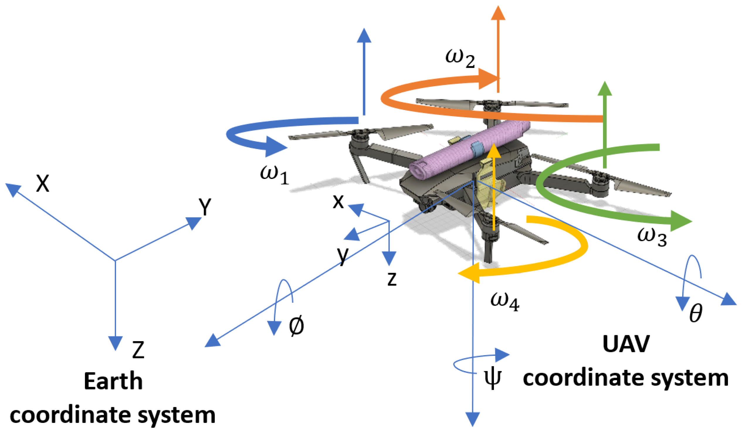
2.1. Reliability and Flight Dynamics of the Chosen UAV in a Specific Mountain Area—The Base for Simulation and Evaluation of the Success of the UAV Flights and Precise Landings
- —is the change in altitude;
- —is the change in roll;
- —is the change in pitch;
- —is the change in yaw;
- —is the aerodynamic thrust coefficient;
- —is the torque moment coefficient;
- —is the angular speed of the propeller.
- —is the change in altitude;
- —is the change in roll;
- —is the change in pitch;
- —is the change in yaw;
- —is the aerodynamic thrust coefficient;
- —is the thrust drag coefficient;
- —is the torque moment coefficient;
- —is the moment drag coefficient
- l—is the length of the arm of the UAV;
- —is the moment of inertia;
- —is the moment of inertia of the motor;
- m—is the mass of the UAV.
2.2. Probabilistic Monitoring of the Coherence of the UAV Flight and the Possibility of Its Accurate Landing at the Reference Point (SLA) in a Mountainous Area—The Base for Simulation and Evaluation of the Success of the UAV Flights and Precise Landings
- —is the coefficient of dangerous UAV landing situations in the mountainous area;
- —is the coefficient of emergency situations causing failed UAV landings in the mountainous area;
- —is the coefficient of catastrophic situations when the UAV unsuccessfully lands in a mountainous area, which leads to its destruction;
- —is the number of dangerous situations during the flight of the UAV caused by the environment;
- —is the number of dangerous situations caused by the surroundings of the UAV landing area in the mountains;
- —is the number of UAV dangerous situations in the mountainous area;
- —is the number of UAV emergency situations in the mountainous area;
- —is the number of UAV catastrophic situations in the mountainous area.
- —is the probability of occurrence of dangerous UAV states in the mountainous area;
- —is the probability of occurrence of emergency UAV states in the mountainous area;
- —is the probability of occurrence of catastrophic UAV states in the mountainous area;
- —is the total probability of occurrence of an extraordinary situation of a UAV when landing in a mountainous area;
- —is the number of UAV dangerous situations in the mountainous area;
- —is the number of UAV emergency situations in the mountainous area;
- —is the number of UAV catastrophic situations in the mountainous area;
- —is the number of UAV flights in the mountainous area realised in the monitored time period.
- —is the probability of occurrence of catastrophic UAV states in the mountainous area;
- —is the coefficient of dangerous UAV landing situations in the mountainous area;
- —is the coefficient of emergency situations causing failed UAV landings in the mountainous area;
- —is the coefficient of catastrophic situations when the UAV unsuccessfully lands in a mountainous area, which leads to its destruction;
- —is the total coefficient of UAV extraordinary situations during landing in the mountainous area;
- —is the total probability of occurrence of an extraordinary situation of a UAV when landing in a mountainous area.
- —is the immediate influence that affects the chain UAV–pilot-operator;
- —is the influence that affects the chain UAV–pilot-operator;
- —is the external condition affecting UAV landing in mountainous areas;
- —is the intersection of factors and , which co-occur, or when one of the conditions occurs (15):
- —is the external condition affecting UAV landing in mountainous areas;
- —is the -th external condition that affects UAV landing in mountainous areas;
- —is the unification of individual partial conditions.
- —is the immediate negative influence that affects the chain UAV–pilot-operator;
- —is the negative influence that affects the chain UAV–pilot-operator;
- —is the negative external condition affecting UAV landing in mountainous areas;
- —is the immediate influence that affects the chain UAV–pilot-operator;
- —is the unification of individual partial conditions;
- —is the empty set.
- —is the probability of occurrence of the extraordinary situation;
- —is the negative influence that affects the chain UAV–pilot-operator;
- —is the negative external condition affecting UAV landing in mountainous areas.
- —is the probability of occurrence of an extraordinary situation;
- —is the negative external condition affecting UAV landing in mountainous areas;
- —is the immediate negative influence that affects the chain UAV–pilot-operator.
- —is the probability of occurrence of dangerous UAV states in the mountainous area;
- —is the probability of occurrence of an extraordinary situation;
- —is the influence that affects the chain UAV–pilot-operator.
- —is a set of possible flight parameters of the UAV in the determined mountain area in the monitored time;
- —is the angle of attack of the UAV in the determined mountain area in the monitored time;
- —is the magnetic heading of the UAV in the determined mountain area in the monitored time;
- —is the flight speed of the UAV in the determined mountain area in the monitored time;
- —is the flight height of the UAV in the determined mountain area in the monitored time;
- —is the -axis position of the UAV in the determined mountain area in the monitored time;
- —is the -axis position of the UAV in the determined mountain area in the monitored time;
- —is the -axis position of the UAV in the determined mountain area in the monitored time.
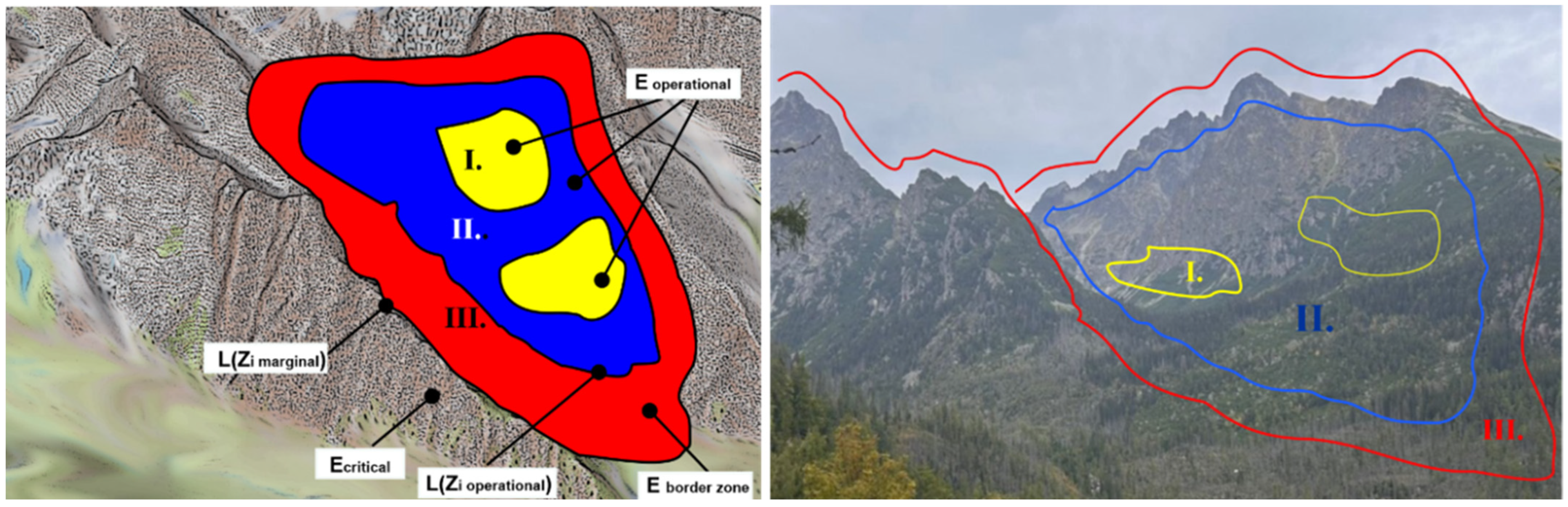
- —is the area (zone) in a mountainous environment in which acceptable UAV flight parameters may be exceeded;
- —is the area (zone) in a mountainous environment with normal UAV flight parameters.
- —is the area (zone) in a mountainous environment with normal UAV flight parameters;
- —is the area (zone) in a mountainous environment in which acceptable UAV flight parameters may be exceeded;
- —is the area (zone) in a mountainous environment with marginal UAV flight parameters.
- —is the area (zone) in a mountainous environment in which acceptable UAV flight parameters may be exceeded;
- —is the area (zone) in a mountainous environment with marginal UAV flight parameters.
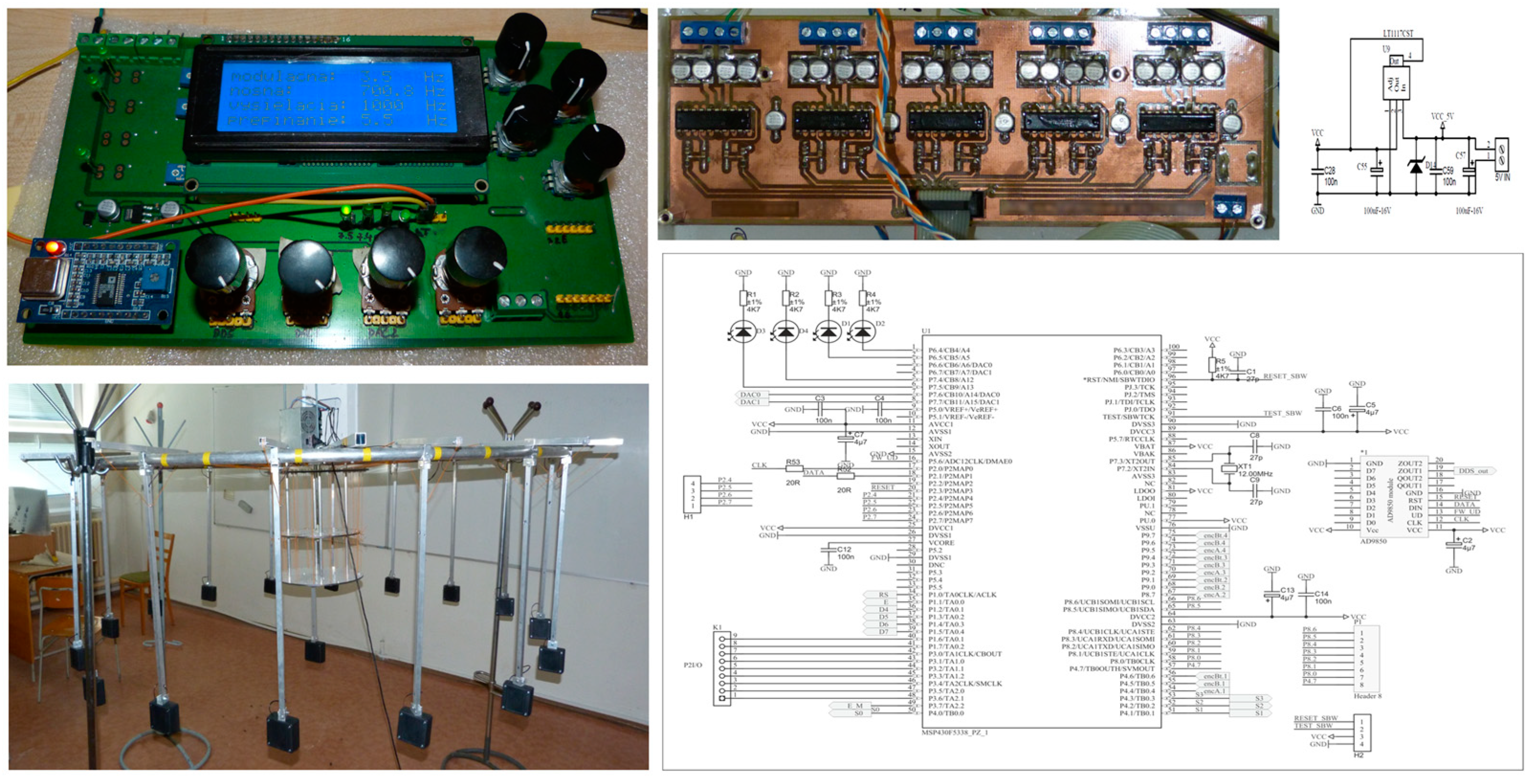
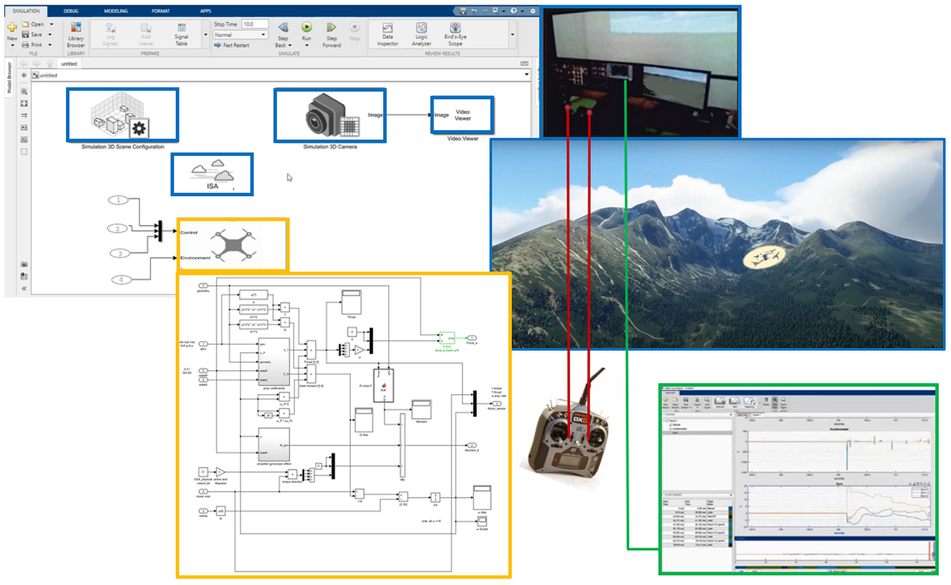
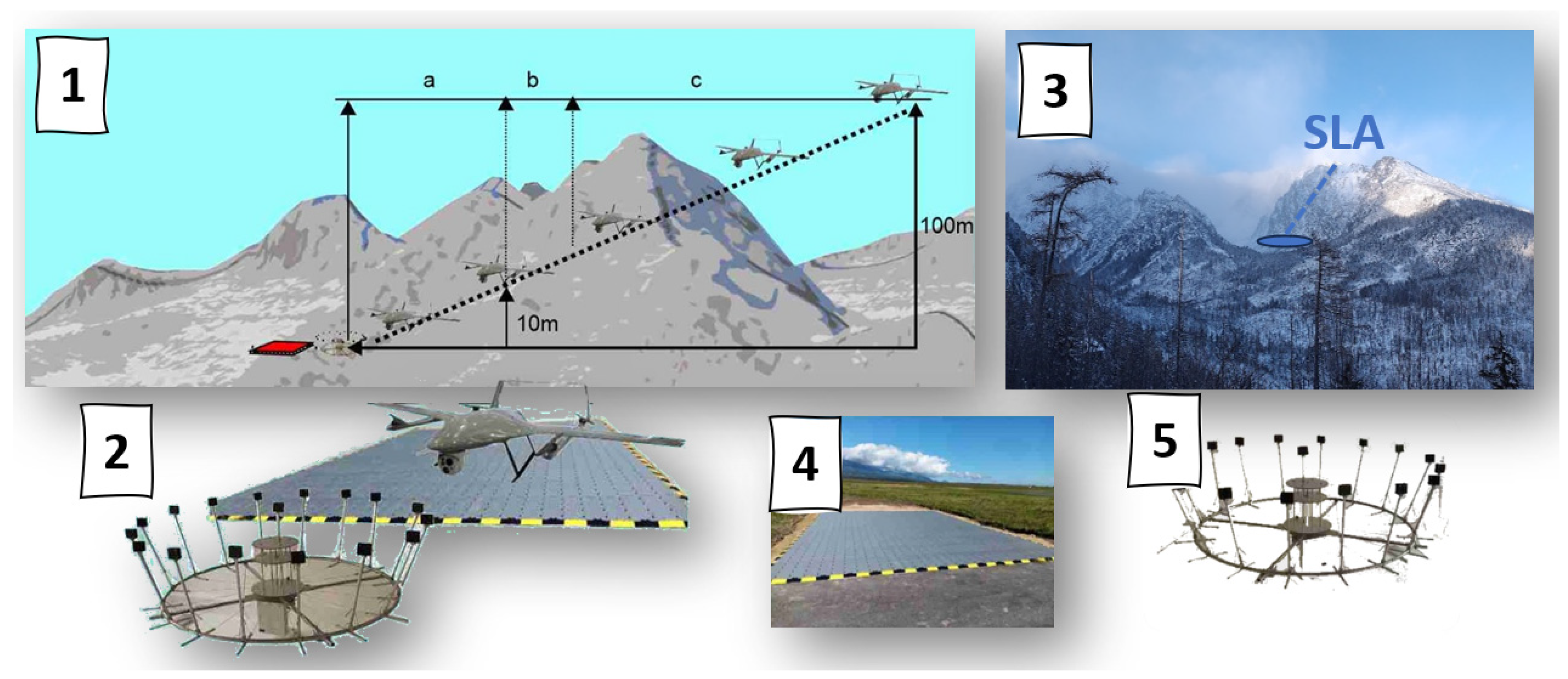
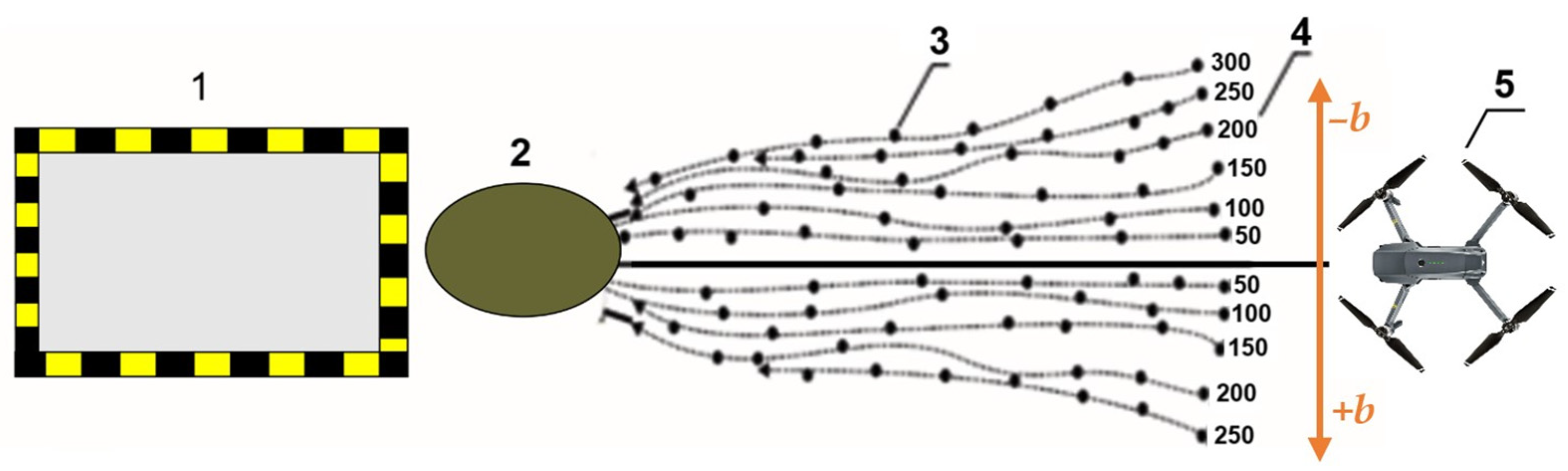
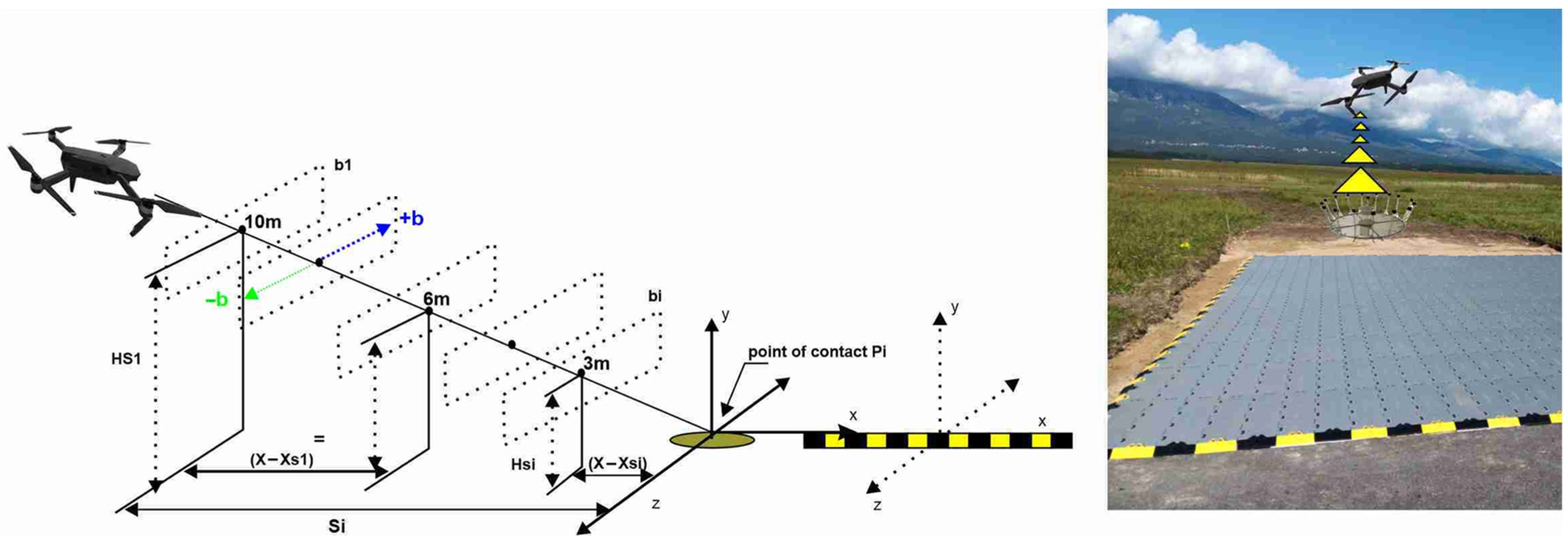
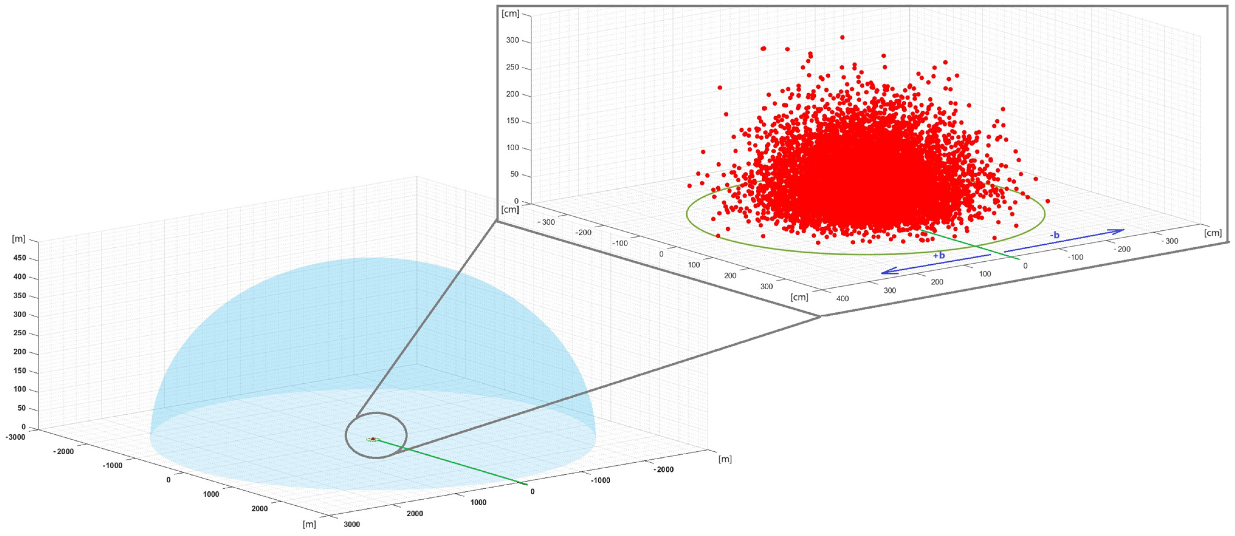
2.3. Simulation and Evaluation Environment of the Success of a Simulated UAV Landing in a Mountainous Area Using the FDLS
- The UAV flight takes place over specified points (coordinates [x,y,z]) at a specific time, with an altitude error of ;
- A flight over specified points located at a specified distance (Figure 6) from the point of approach and final landing of the UAV to the experimental landing area located behind the FDLS, which must be realised in time with a time variance of .
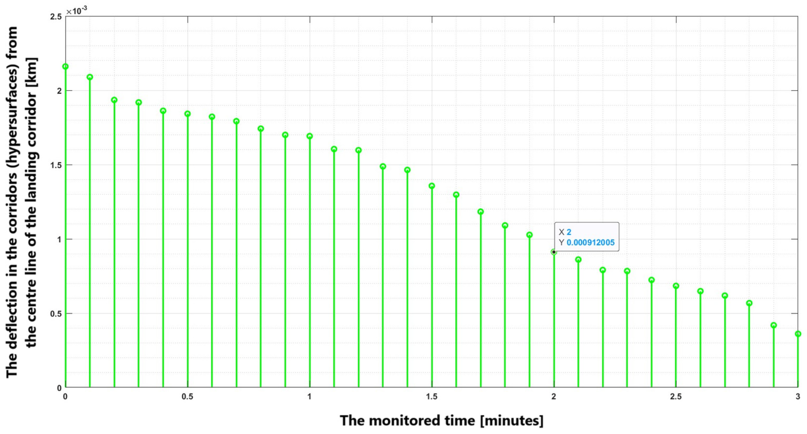
3. Results and Discussion
- —is the point of touch (interest) of the UAV at the experimental landing area;
- —is the horizontal width of the defined corridor (hypersurface);
- —is the defined corridor (hypersurface);
- —is the current flight height of the UAV above the terrain;
- –is the distance of the UAV’s centre of gravity position from the point of touch (interest) at the experimental landing area;
- —is the lateral (horizontal) deviation from the ideal line (landing trajectory) of the UAV;
- —is the descent (vertical) deviation from the ideal line (landing trajectory) of the UAV;
- —is the ground distance between the actual position of the UAV and the point of touch (interest) placed at the experimental landing area located behind the FDLS.
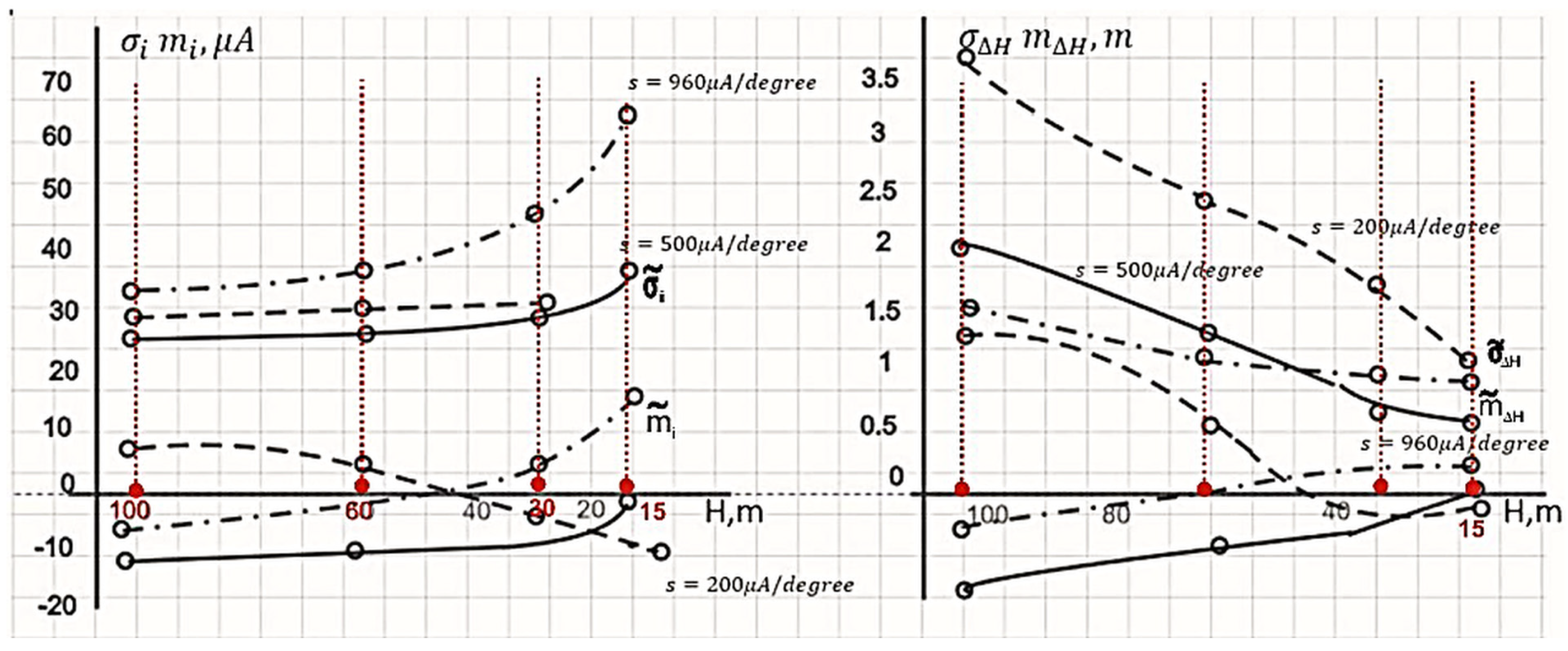
- —is the dispersion of the measurement error of the horizontal coordinate at the time ;
- —is the dispersion of the error of the measured time ;
- —is the root-mean-squared deviation.
- —is the distance of the UAV’s centre of gravity position from the point of touch (interest) at the experimental landing area;
- —is the current flight height of the UAV above the terrain;
- —is the lateral (horizontal) deviation from the ideal line (landing trajectory) of the UAV;
- —is the ground distance between the actual position of the UAV and the point of touch (interest) placed at the experimental landing area located behind the FDLS.
- —is the probability of UAV movement at the level , i.e., from the ideal line of the landing corridor generated by the FDLS to the left of the ideal point of contact with the experimental landing area;
- —is the probability of UAV movement at the level , i.e., from the ideal line of the landing corridor generated by the FDLS to the right of the ideal point of contact with the experimental landing area;
- —is a function of the standardised normal distribution;
- —is the horizontal width of the defined corridor (hypersurface);
- —is the root-mean-squared deviation;
- —is the initial time in the first section of the measurement;
- —is the time shift in the measurement section.
4. Conclusions
Author Contributions
Funding
Data Availability Statement
Acknowledgments
Conflicts of Interest
References
- ICAO Annex 14—Aerodromes. Available online: https://www.icao.int/safety/airnavigation/nationalitymarks/annexes_booklet_en.pdf (accessed on 8 September 2023).
- Öktemer, E.; Gültekin, E.E. Operational usage and importance of instrument landing system (ILS). Int. J. Aeronaut. Astronaut. 2021, 2, 18–21. [Google Scholar]
- Lopez, A.R. GPS Landing System Reference Antenna. IEEE Antennas Propag. Mag. 2010, 52, 104–113. [Google Scholar] [CrossRef]
- Gross, J.N.; Gu, Y.; Rhudy, M.B. Robust UAV Relative Navigation with DGPS, INS, and Peer-to-Peer Radio Ranging. IEEE Trans. Autom. Sci. Eng. 2015, 12, 935–944. [Google Scholar] [CrossRef]
- Felux, M.; Dautermann, T.; Becker, H. GBAS landing system—Precision approach guidance after ILS. Aircr. Eng. Aerosp. Technol. 2013, 85, 382–388. [Google Scholar] [CrossRef]
- Cho, A.; Kang, Y.-S.; Park, B.-J.; Yoo, C.-S.; Koo, S.-O. Altitude integration of radar altimeter and GPS/INS for automatic takeoff and landing of a UAV. In Proceedings of the 11th International Conference on Control, Automation and Systems, Gyeonggi-do, Republic of Korea, 26–29 October 2011. [Google Scholar]
- Klochan, A.E.; Al-Ammouri, A.; Dekhtyar, M.M.; Poleva, N.M. Fundamentals of the Polarimetric UAV Landing System. In Proceedings of the IEEE 5th International Conference Actual Problems of Unmanned Aerial Vehicles Developments (APUAVD), Kiev, Ukraine, 22–24 October 2019; pp. 153–156. [Google Scholar] [CrossRef]
- Naidoo, Y.; Stopforth, R.; Bright, G. Development of an UAV for search & rescue applications. In Proceedings of the IEEE Africon ‘11, Victoria Falls, Zambia, 13–15 September 2011; pp. 1–6. [Google Scholar] [CrossRef]
- Liu, Z.; Chen, H.; Wen, Y.; Xiao, C.; Chen, Y.; Sui, Z. Mode Design and Experiment of Unmanned Aerial Vehicle Search and Rescue in Inland Waters. In Proceedings of the 6th International Conference on Transportation Information and Safety (ICTIS), Wuhan, China, 22–24 October 2021; pp. 917–922. [Google Scholar] [CrossRef]
- Ashish, M.; Muraleedharan, A.; CM, S.; Bhavani, R.R.; Akshay, N. Autonomous Payload Delivery using Hybrid VTOL UAVs for Community Emergency Response. In Proceedings of the IEEE International Conference on Electronics, Computing and Communication Technologies (CONECCT), Bangalore, India, 2–4 July 2020; pp. 1–6. [Google Scholar] [CrossRef]
- Rudol, P.; Doherty, P. Human Body Detection and Geolocalization for UAV Search and Rescue Missions Using Color and Thermal Imagery. In Proceedings of the IEEE Aerospace Conference, Big Sky, MT, USA, 1–8 March 2008; pp. 1–8. [Google Scholar] [CrossRef]
- ter Avest, E.; Kratz, M.; Dill, T.; Palmer, M. HEMS in mountain and remote areas: Reduction of carbon footprint through drones. Scand. J. Trauma Resusc. Emerg. Med. 2023, 31, 73. [Google Scholar] [CrossRef] [PubMed]
- Claesson, A.; Fredman, D.; Svensson, L. Unmanned aerial vehicles (drones) in out-of-hospital-cardiac-arrest. Scand. J. Trauma Resusc. Emerg. Med. 2016, 24, 124. [Google Scholar] [CrossRef] [PubMed]
- Yan, X.; Fu, T.; Lin, H.; Xuan, F.; Huang, Y.; Cao, Y.; Hu, H.; Liu, P. UAV Detection and Tracking in Urban Environments Using Passive Sensors: A Survey. Appl. Sci. 2023, 13, 11320. [Google Scholar] [CrossRef]
- Salom, I.; Dimić, G.; Čelebić, V.; Spasenović, M.; Raičković, M.; Mihajlović, M.; Todorović, D. An Acoustic Camera for Use on UAVs. Sensors 2023, 23, 880. [Google Scholar] [CrossRef] [PubMed]
- Yousaf, J.; Zia, H.; Alhalabi, M.; Yaghi, M.; Basmaji, T.; Shehhi, E.A.; Gad, A.; Alkhedher, M.; Ghazal, M. Drone and Controller Detection and Localization: Trends and Challenges. Appl. Sci. 2022, 12, 12612. [Google Scholar] [CrossRef]
- Češkovič, M.; Kurdel, P.; Gecejová, N.; Labun, J.; Gamcová, M.; Lehocký, M. A Reasonable Alternative System for Searching UAVs in the Local Area. Sensors 2022, 22, 3122. [Google Scholar] [CrossRef] [PubMed]
- Hussain, A.; Ahmed, A.; Shah, M.A.; Katyara, S.; Staszewski, L.; Magsi, H. On Mitigating the Effects of Multipath on GNSS Using Environmental Context Detection. Appl. Sci. 2022, 12, 12389. [Google Scholar] [CrossRef]
- Iliev, T.B.; Stoyanov, I.S.; Sokolov, S.A.; Beloev, I.H. The Influence of Multipath Propagation of the Signal on the Accuracy of the GNSS Receiver. In Proceedings of the 43rd International Convention on Information, Communication and Electronic Technology (MIPRO), Opatija, Croatia, 28 September–2 October 2020; pp. 508–511. [Google Scholar] [CrossRef]
- Abdulkareem, A.; Oguntosin, V.; Popoola, O.M.; Idowu, A.A. Modeling and Nonlinear Control of a Quadcopter for Stabilization and Trajectory Tracking. J. Eng. 2022, 2022, 2449901. [Google Scholar] [CrossRef]
- Wang, P.; Man, Z.; Cao, Z.; Zheng, J.; Zhao, Y. Dynamics modelling and linear control of quadcopter. In Proceedings of the 2016 International Conference on Advanced Mechatronic Systems (ICAMechS), Melbourne, Australia, 30 November–3 December 2016. [Google Scholar] [CrossRef]
- Ahmad, F.; Kumar, P.; Bhandari, A.; Patil, P.P. Simulation of the Quadcopter Dynamics with LQR based Control. Mater. Today Proc. 2020, 24, 326–332. [Google Scholar] [CrossRef]
- Tagay, A.; Omar, A.; Ali, M.H. Development of control algorithm for a quadcopter. Procedia Comput. Sci. 2021, 179, 242–251. [Google Scholar] [CrossRef]
- Quadcopter Flight Mechanics Model and Control Algorithms. Available online: https://wiki.control.fel.cvut.cz/mediawiki/images/5/5e/Dp_2017_gopalakrishnan_eswarmurthi.pdf (accessed on 1 October 2023).
- Kurdel, P.; Češkovič, M.; Gecejová, N.; Adamčík, F.; Gamcová, M. Local Control of Unmanned Air Vehicles in the Mountain Area. Drones 2022, 6, 54. [Google Scholar] [CrossRef]
- Onicha, J.N. Advanced Mathematica, 1st ed.; CreateSpace Independent Publishing Platform: Scotts Valley, CA, USA, 2014; pp. 131–243, 457–498. [Google Scholar]
- Introduction to Mathematical Statistics. Available online: https://minerva.it.manchester.ac.uk/~saralees/statbook2.pdf (accessed on 10 October 2023).
- Freund, J.E. Mathematical Statistics with Applications, 8th ed.; Pearson: London, UK, 2012; pp. 61–112. [Google Scholar]
- Seier, G.; Hödl, C.; Abermann, J.; Schöttl, S.; Maringer, A.; Hofstadler, D.N.; Pröbstl-Haider, U.; Lieb, G.K. Unmanned aircraft systems for protected areas: Gadgetry or necessity. J. Nat. Conserv. 2021, 64, 126078. [Google Scholar] [CrossRef]
- Pikov, V.; Ryapukhin, A.; Veas Iniesta, D. Information Protection in Complexes with Unmanned Aerial Vehicles Using Moving Target Technology. Inventions 2023, 8, 18. [Google Scholar] [CrossRef]
- Kang, H.; Joung, J.; Kim, J.; Kang, J.; Cho, Y.S. Protect Your Sky: A Survey of Counter Unmanned Aerial Vehicle Systems. IEEE Access 2020, 8, 168671–168710. [Google Scholar] [CrossRef]
- Ripley, B.D. Feed-forward Neural Networks. In Pattern Recognition and Neural Networks, 1st ed.; Cambridge University Press: Cambridge, UK, 1996; pp. 143–180. [Google Scholar] [CrossRef]
- Aggarwal, C.C. Neural Networks and Deep Learning, 1st ed.; Springer: Cham, Switzerland, 2018; pp. 1–104. [Google Scholar] [CrossRef]
- Dobeš, M.; Andoga, R.; Főző, L. Sensory integration in deep neural networks. Acta Polytech. Hung. 2021, 18, 245–254. [Google Scholar] [CrossRef]


| UAV flight speed during the final phase of the approach to landing and landing itself. | 55 km/h |
| The time duration of the final phase of the approach to landing and the landing itself. | 3 min = 180 s |
| The distance for interception and navigation of the UAV, with the navigation signals from the FDLS, for navigation to the final phase of the landing approach and the landing itself. | 2.75 km = 2750 m |
| Permitted width of horizontal deviation (±b) of the UAV in the defined corridor (hypersurface) in the determined area—the Little Cold Valley, High Tatras. | ±3 m = ±300 cm |
Disclaimer/Publisher’s Note: The statements, opinions and data contained in all publications are solely those of the individual author(s) and contributor(s) and not of MDPI and/or the editor(s). MDPI and/or the editor(s) disclaim responsibility for any injury to people or property resulting from any ideas, methods, instructions or products referred to in the content. |
© 2024 by the authors. Licensee MDPI, Basel, Switzerland. This article is an open access article distributed under the terms and conditions of the Creative Commons Attribution (CC BY) license (https://creativecommons.org/licenses/by/4.0/).
Share and Cite
Kurdel, P.; Gecejová, N.; Češkovič, M.; Yakovlieva, A. Evaluation of the Success of Simulation of the Unmanned Aerial Vehicle Precision Landing Provided by a Newly Designed System for Precision Landing in a Mountainous Area. Aerospace 2024, 11, 82. https://doi.org/10.3390/aerospace11010082
Kurdel P, Gecejová N, Češkovič M, Yakovlieva A. Evaluation of the Success of Simulation of the Unmanned Aerial Vehicle Precision Landing Provided by a Newly Designed System for Precision Landing in a Mountainous Area. Aerospace. 2024; 11(1):82. https://doi.org/10.3390/aerospace11010082
Chicago/Turabian StyleKurdel, Pavol, Natália Gecejová, Marek Češkovič, and Anna Yakovlieva. 2024. "Evaluation of the Success of Simulation of the Unmanned Aerial Vehicle Precision Landing Provided by a Newly Designed System for Precision Landing in a Mountainous Area" Aerospace 11, no. 1: 82. https://doi.org/10.3390/aerospace11010082
APA StyleKurdel, P., Gecejová, N., Češkovič, M., & Yakovlieva, A. (2024). Evaluation of the Success of Simulation of the Unmanned Aerial Vehicle Precision Landing Provided by a Newly Designed System for Precision Landing in a Mountainous Area. Aerospace, 11(1), 82. https://doi.org/10.3390/aerospace11010082