Fixed-Wing UAV Formation Path Planning Based on Formation Control: Theory and Application

Abstract

Formation path planning is a significant cornerstone for unmanned aerial vehicle (UAV) swarm intelligence. Previous methods were not suitable for large-scale UAV formation, which suffered from poor formation maintenance and low planning efficiency. To this end, this paper proposes a novel millisecond-level path planning method appropriate for large-scale fixed-wing UAV formation, which consists of two parts. Instead of directly planning paths independently for each UAV in the formation, the proposed method first introduces a formation control strategy. It controls the chaotic UAV swarm to move as a single rigid body, so that only one planning can obtain the feasible path of the entire formation. Then, a computationally lightweight Dubins path generation method with a closed-form expression is employed to plan feasible paths for the formation. During flight, the aforementioned formation control strategy maintains the geometric features of the formation and avoids internal collisions within the formation. Finally, the effectiveness of the proposed framework is exemplified through several simulations. The results show that the proposed method can not only achieve millisecond-level path planning for the entire formation but also excellently maintain formation during the flight. Furthermore, simple formation obstacle avoidance in a special case also highlights the application potential of the proposed method.

1. Introduction

Due to the advantages of large scale, long endurance, and heavy load, the fixed-wing unmanned aerial vehicle (UAV) formation can efficiently complete large-scale disaster search and rescue [1,2], long-term monitoring of the ecological environment [3,4], and continuous battlefield monitoring and aerobatics [5]. According to the mission requirements and environmental constraints, a group of fixed-wing UAVs form a specific formation in accordance with the desired bearing and distance. They then need to maintain this formation while flying from one waypoint to another, each with a specified attitude. These are crucial parts of the path planning for fixed-wing UAV formation. Numerous existing articles [6,7,8,9] have investigated the formation path planning (FPP) of fixed-wing UAV with diverse methods. Although it has been studied, formation-keeping path planning still presents some attractive challenges that are poorly addressed.

One challenge lies in the assembly and maintenance of large-scale UAV formation. First, a UAV swarm with as many as a dozen fixed-wing UAVs needs to reliably complete the formation assembly and establish the desired formation geometric characteristics (shape, distance, angle, etc.). More importantly, the UAV swarm needs to maintain the desired formation while traveling from the start to the target, enabling the swarm to move like a single rigid body. This characteristic is particularly appealing in certain real-world scenarios. However, existing research on fixed-wing UAV often neglect the challenge of maintaining the formation geometric characteristics during path flight.

Another challenge of formation-keeping path planning is fast planning. On the one hand, existing research employs optimization-based methods, potential field methods and intelligent evolution-based algorithms to plan the path. These methods commonly involve performing formation path planning independently for each UAV in the formation, resulting in the number of path planning instances being equal to the number of UAVs. Therefore, for large formation scales, this can impact planning efficiency. On the other hand, optimization-based methods and intelligent evolution-based algorithms make the path planning of each UAV inefficient due to their inherent characteristics. To sum up, achieving fast formation path planning while maintaining the formation is a thorny problem.

Motivated by the above-mentioned challenges, this paper investigates a novel, efficient path planning method or framework for large-scale distributed fixed-wing UAV formation. Its distinct feature is that it comprises two parts: formation control and path generation. The schematic of its architecture is shown in Figure 1. The contributions of this paper are threefold.

Firstly, to drive a group of UAVs to form and maintain desired geometric characteristics, a formation control method with multiple functions is introduced. Currently, numerous formation control methods have been proposed, including distance-based (DB) [10], barycentric coordinate-based (BCB) [11], bearing-based (BB) formation control methods [12], and their combination methods [13,14]. To ensure convergence of UAVs from any initial conditions to the desired formation and control the formation scale, this paper employs a hybrid formation control method. In addition to completing the formation assembly, the formation control method not only maintains the geometric characteristics during flight but also ensures collision avoidance among the UAVs within the formation. The validity of the control law is demonstrated using the Lyapunov stability principle.

Secondly, this paper suggests a Dubins path generation method based on analytic geometry to achieve fast and optimal path planning. Following the implementation of formation control, all fixed-wing UAVs within the formation are in the same motion state, thus treating the UAV formation as a single large fixed-wing UAV. In this way, a single path generation is enough to obtain a feasible path for the entire formation, greatly improving planning efficiency. A two-dimensional Dubins path optimization problem is formulated to obtain the optimal path. However, considering the large distance between the start and target of the fixed-wing UAV, the method generates an optimal path using a geometric method instead of solving the optimal control problem. This approach enables path planning within milliseconds. The feasibility of the proposed path planning method is verified through simulation experiments.

Thirdly, to showcase the application potential of the proposed method in formation obstacle avoidance, this paper presents a simple approach for formation obstacle avoidance in a specific situation. The path planned by the proposed method is inherently smooth as it satisfies the kinematic characteristics of the fixed-wing UAV and requires no further optimization. Additionally, its fast-planning characteristic makes it well suited for obstacle avoidance path planning. We focus on a specific obstacle avoidance situation where the path planned for an individual UAV can also facilitate obstacle avoidance for the entire UAV swarm. The obstacle avoidance strategy involves rapidly generating candidate paths and subsequently optimizing them to circumvent obstacles.

The paper is organized as follows. A literature review is presented in Section 2. In Section 3, the UAV model and formation path planning scenario are discussed. In Section 4, the overview and framework of the proposed method are elaborated, including the distributed control law and its proof, Dubins path generation method, and obstacle avoidance strategy. Numerical simulations in Section 5 demonstrate the viability of formation control and path planning method, and show the potential of path planning methods for obstacle avoidance. The main findings of this work are summarized in Section 6, and suggestions for further progress are made.

2. Related Works

FPP refers to finding a feasible path for the UAV swarm from the initial point to the target point without causing internal collisions and violating kinematic constraints while optimizing path performance. There are numerous methods based on various principles that can be employed to tackle this issue, which have been extensively researched in the literature.

We classify and evaluate the relevant literature according to different methods. Firstly, we delve into the optimization-based approaches. To generate independent and separate paths for each UAV and guarantee collision-free operation within the formation, Kaminer et al. [15] studied a multi-UAV coordination control method based on optimization theory. Choe et al. [16] presented a heuristic method to solve the multi-mission UAV trajectory generation problem. The path generation problem was also transformed into a constrained optimization problem. Additionally, the Pythagorean Hodograph Bezier curve was used to generate a feasible path that satisfies the kinematic constraints of the UAV. With the widespread attention paid to the pseudospectral method in the field of trajectory planning, Zhou et al. [6] proposed a method for solving the fixed-wing UAV formation trajectory planning problem based on the Gaussian pseudospectral method, and discussed the formation conversion and formation maintenance during formation flight. Wang et al. [8] developed a formation path planning algorithm based on the multi-phase adaptive pseudospectral method. This method took into full consideration the constraints on heading angular rate and linear velocity when generating a feasible set of formation heading speeds. Generally, in existing optimization-based path planning methods, the number of UAVs is typically small, and the formations are relatively simple.

Then, the methods based on intelligent, artificial potential field and other methods are reviewed. To solve the problem of path planning for small-scale UAVs in radar-threat environments, Chen et al. [17] proposed a 3D path planning method for UAV formation based on the ant colony optimization algorithm. Shao et al. [9] suggested a 3D path planning algorithm for UAV formation based on a comprehensive improved particle swarm optimization algorithm. The algorithm has been improved in three aspects of initialization, adaptive varying parameters, and mutation update strategy, so as to speed up the convergence and improve the solution optimality. Zhang et al. [7] developed a real-time path planning method for UAV swarms based on the improved artificial potential field method. This method accomplished not only path planning but also the control of formation shape and distance by employing the artificial potential field method. Recently, the integer programming has also been introduced into formation path planning problems. Luciano et al. [18] presented an optimization method for fixed-wing UAV formation trajectory planning based on graph theory and clothoid curves, while solving the mixed integer optimal control problem of the formation to avoid collisions between UAVs. With the rapid development of machine learning technology, numerous researchers have adopted machine learning methods for path planning. Specifically, Arani et al. [19] utilized reinforcement learning methods to devise path planning strategies for drones. Cristian et al. [20] employed a supervised learning method to address the Markov–Dubins problem, thereby determining a feasible path for fixed-wing UAV. Additionally, conventional geometric path-planning methods can be adapted for FPP. The Dubins curve [21,22] is commonly employed in path planning due to its compatibility with the minimum turning radius constraints of fixed-wing UAVs. However, its application to large-scale UAV swarms has been limited by challenges related to obstacle avoidance both within and outside the formation.

In summary, existing research have concentrated on path planning for small-scale fixed-wing UAV formation. The formations typically comprise a restricted number of UAVs characterized by simplistic geometries and loosely maintained formations, thereby precluding the possibility of the entire UAV swarm exhibiting movement akin to that of a rigid body. Moreover, the planning efficiency leaves room for improvement. It is clear that developing an ad hoc solution to overcome these challenges may lead to better solutions.

3. Problem Statement

In this section, the single fixed-wing UAV model is first presented. The model is then transformed into an equivalent single-integral model through parameter transformation, enabling the application of the hybrid formation control law. Finally, the formation path planning scenario for fixed-wing UAV is briefly illustrated.

3.1. Single Fixed-Wing UAV Model and Distributed Control Model

Figure 2 displays the undirected graph of the UAV formation, where the UAVs are connected by solid lines to indicate that they can communicate with each other and are therefore considered neighbors. The desired formation is achieved when all distances and angles between each UAV and its neighbors match the desired configuration.

The i-th fixed-wing UAV in the UAV formation is modeled by a planar nonholonomic vehicle, generally known as a unicycle. Compared with the complex six-degree-of-freedom model, it is more suitable for high-level formation control and path planning because it does not take into account factors such as aerodynamics and wind disturbance. Its kinematic model can be written as follows:

$$\left\{\begin{array}{c}{\dot{x}}_i=v_i\cos \left({\psi }_i\right),\hfill \\ {\dot{y}}_i=v_i\sin \left({\psi }_i\right),\hfill \\ {\dot{\psi }}_i={\omega }_i.\hfill \end{array}\right.$$

(1)

where $x,y$ denote the position of the UAV in the inertial coordinate system $\left(OXY\right)$, v denotes the airspeed of the UAV, $\psi$ denotes the heading angle of the aircraft, that is, the angle between the x-axis and the speed vector v, which is positive when measured counterclockwise, and $\omega$ denotes the angular velocity of the UAV heading angle. Due to the limitation of power and roll angle, its airspeed and angular velocity of heading angle are also limited accordingly, expressed as

$$\begin{array}{c}{v}_{min}\le {\nu }_i\le {\nu }_{max},\\ \mid {\omega }_i\mid \le {\omega }_{max}.\end{array}$$

(2)

The minimum turning radius is a critical flight performance metric for UAV, which plays a crucial role in planning the optimal path. During flight, the UAV often maintains a constant speed. In such instances, the minimum turning radius is determined by the maximum value of the heading angular velocity.

Numerical formation control methods developed previously have relied on the single-integral model. To incorporate mature formation control laws, the model of fixed-wing UAV needs to transform into an equivalent single-integral model through parameter conversion. The heading vector ${\mathit{h}}_{\mathit{i}}$ and its vertical vector ${\mathit{h}}_{\mathit{i}}^{\mathit{p}}$ are defined as

$${\mathit{h}}_{\mathit{i}}=\left[\begin{array}{c}\cos \left({\psi }_i\right)\\ \sin \left({\psi }_i\right)\end{array}\right],{\mathit{h}}_{\mathit{i}}^p=\left[\begin{array}{c}-\sin \left({\psi }_i\right)\\ \cos \left({\psi }_i\right)\end{array}\right].$$

(3)

In this way, the fixed wing UAV model (1) can be rewritten as

$$\begin{array}{cc}\hfill {\dot{\mathit{q}}}_i& ={\mathit{h}}_{\mathit{i}}{v}_i,\hfill \\ \hfill {\dot{\mathit{h}}}_i& ={\mathit{h}}_{\mathit{i}}^p{\omega }_i,\hfill \end{array}$$

(4)

where ${\mathit{q}}_{\mathit{i}}={\left[x_i,y_i\right]}^T\in {\mathbb{R}}^2$ is the position of the UAV in the global coordinate system.

3.2. Formation Path Planning Scenario

This study aims to develop a novel formation path planning method that can be performed properly and quickly, maintain the desired formation geometric characteristics, and reach the desired destination B (shown as a black dot). The problem scenario is shown in Figure 3. A swarm of UAVs initially transitions from chaotic state 1 to starting point A, simultaneously forming the desired formation state 2. The formation then swiftly advances from the starting point A, following the shortest path at a designated heading angle, toward target point B. During this period, the UAV swarm consistently maintains its desired geometric formation. Throughout the flight, the UAV swarm actively avoids internal collisions to ensure safety.

The problem is considered as two-dimensional, assuming there are no obstacles in the air. Discussion of scenarios with static obstacles will follow in the section on obstacle avoidance strategies. All UAVs in the formation are homogeneous, equipped with GPS and IMU for precise positioning. Additionally, they can communicate with specific neighboring UAVs within the formation.

4. Implementation Details

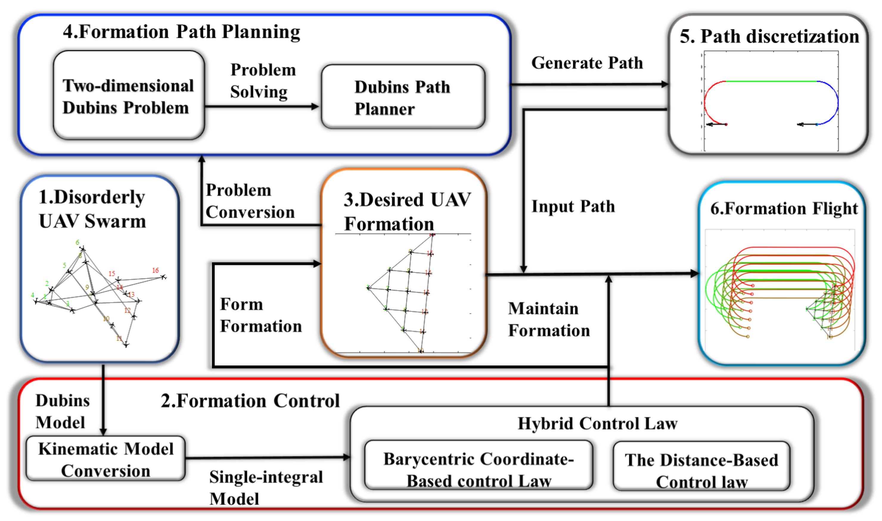
The solution to the formation path planning problem is twofold: formation control and path planning. The former employs hybrid formation control laws to control the chaotic UAV swarm into a desired formation, allowing it to behave as a single rigid body. For the latter, we utilize the Dubins path generation method based on analytical geometry to swiftly devise an optimal feasible path. Furthermore, we discuss the problem of obstacle avoidance under a special condition and propose specific strategies.

4.1. Distributed Control Law

By introducing formation control, the complex problem of formation path planning is transformed into a single UAV path planning problem. Therefore, we shall initially discuss the formation control methods. It is evident that the linear velocity and angular velocity in (4) serve as control parameters. During the formation control stage, the fixed-wing UAV is required to complete two tasks: forming the desired formation and moving towards the starting point of formation path flight along the specified direction. Hence, the control parameters should also incorporate two components: formation control and expected speed,

$$\begin{array}{c}{v}_i={\mathit{h}}_{\mathit{i}}^T({\mathit{u}}_{\mathit{i}}+c{\mathit{p}}_{\mathit{i}}),\\ {\omega }_i={\mathit{h}}_{\mathit{i}}^{p^T}({\mathit{u}}_{\mathit{i}}+c{\mathit{p}}_{\mathit{i}}).\end{array}$$

(5)

where ${\mathit{p}}_{\mathit{i}}$ denotes the unit velocity vector, $c>0$ denotes the desired velocity, and ${\mathit{u}}_{\mathit{i}}$ is the hybrid control law as follow:

$$\begin{array}{cc}\hfill & {\mathit{u}}_{\mathit{i}\mathit{1}}=\sum _{j\in {\mathbb{N}}_i}{\mathit{A}}_{\mathit{i}\mathit{j}}({\mathit{q}}_{\mathit{j}}-{\mathit{q}}_{\mathit{i}}),\hfill \\ \hfill & {\mathit{u}}_{\mathit{i}\mathbf{2}}=f(d_{ij}-d_{ij}^{*})({\mathit{q}}_{\mathit{j}}-{\mathit{q}}_{\mathit{i}}),\hfill \\ \hfill & {\mathit{u}}_{\mathit{i}}={\mathit{u}}_{\mathit{i}\mathbf{1}}+{\mathit{u}}_{\mathit{i}\mathbf{2}}.\hfill \end{array}$$

(6)

Note that both ${\mathit{u}}_{\mathit{i}}$ and ${\mathit{p}}_{\mathit{i}}$ are given relative to the local coordinate system of the agent and need to be transformed to be projected onto the UAV heading direction ${\mathit{h}}_{\mathit{i}}$ and its vertical vector ${\mathit{h}}_{\mathit{i}}^p$.

The linear term ${\mathit{u}}_{\mathit{i}\mathbf{1}}$ is a control law based on barycentric coordinates, which can ensure that UAVs almost globally converge to the desired formation shape. Here, ${\mathbb{N}}_i$ represents the set of neighbors of agent i, and ${\mathit{A}}_{\mathit{ij}}\in {\mathbb{R}}^{2\times 2}$ is the constant control gain matrix to be given, in the form of

$${\mathit{A}}_{\mathit{ij}}=\left[\begin{array}{cc}{a}_{ij}& b_{ij}\\ -b_{ij}& a_{ij}\end{array}\right].$$

(7)

It should be noted that the main diagonal elements of ${\mathit{A}}_{\mathit{ij}}$ remain identical, but the signs of the subdiagonal elements are opposite. By restricting the gain matrix to this form, the expression of the closed-loop dynamics in global or local coordinate system is guaranteed to be invariant [13]. This not only enables the agent to use the relative positions of neighbors measured in the local coordinate system, but also design and analyze control strategies in the global coordinate system.

Although the control law based on barycentric coordinates guarantees that the UAVs converge to the desired formation shape under almost all initial conditions, it is unable to control the formation scale. Consequently, to determine the final formation scale, it is expanded with the distance-based control law ${\mathit{u}}_{\mathit{i}\mathbf{2}}$, where $d_{ij}=\left|\right|{\mathit{q}}_{\mathit{j}}-{\mathit{q}}_{\mathit{i}}\left|\right|$ denotes the distance between agent i and j, while $d_{ij}^{*}$ denotes their expected distance. f is a bounded smooth map and chosen such that for all $x\in \mathbb{R}$, $xf\left(x\right)>0$ for $x\ne 0$, and $f\left(0\right)=0$. This article selects

$$f={\displaystyle \frac{1}{m}}\arctan \left(x\right),$$

(8)

where $m>0$ is an arbitrary constant, which can be chosen to have a desired $f_{max}$. The augmentation term ${\mathit{u}}_{\mathit{i}\mathbf{2}}$, a distance-based control law, influences agent i to move towards its neighbor j when the distance $d_{ij}$ between agents i and j exceeds the desired distance $d_{ij}^{*}$, and vice versa. This mechanism guarantees collision avoidance among the UAVs within the formation during flight.

In the initial phase of the formation control, the linear item ${\mathit{u}}_{\mathit{i}\mathbf{1}}$ predominates, and the fixed-wing UAVs first move quickly to the desired formation shape. As the UAVs near the formation shape, the augmentation term ${\mathit{u}}_{\mathit{i}\mathbf{2}}$ becomes dominant, and the formation will slowly expand or contract to achieve the desired scale.

4.2. The Closed-Loop Dynamics

By substituting (5) and (6) into (4), the closed-loop dynamics of UAVs can be collectively expressed as:

$$\begin{array}{c}\dot{\mathit{q}}={\mathit{HH}}^T(\mathit{Aq}+\mathit{Fq}+c\mathit{P}),\\ \dot{\mathit{h}}={\mathit{H}}^p{\mathit{H}}^{pT}(\mathit{Aq}+\mathit{Fq}+c\mathit{P}).\end{array}$$

(9)

where $\mathit{q}={[{\mathit{q}}_{\mathbf{1}}^T,{\mathit{q}}_{\mathbf{2}}^T,\dots ,{\mathit{q}}_{\mathit{n}}^T]}^T\in {\mathbb{R}}^{2n}$ denotes the aggregate state vector, $\mathit{P}$ denotes the velocity direction vector of the UAV, which is a constant vector, and $\begin{array}{c}\hfill \mathit{h}={[{\mathit{h}}_{\mathbf{1}}^T,{\mathit{h}}_{\mathbf{2}}^T,\dots ,{\mathit{h}}_{\mathit{n}}^T]}^T\end{array}$ denotes the aggregate heading vector. Matrices $\mathit{H}$ and ${\mathit{H}}^{\mathit{p}}$ are defined as

$$\mathit{H}=\left[\begin{array}{cccc}{\mathit{h}}_{\mathbf{1}}& \mathbf{0}& ...& \mathbf{0}\\ \mathbf{0}& {\mathit{h}}_{\mathbf{2}}& ...& \mathbf{0}\\ ⋮& ⋮& \ddots & ⋮\\ \mathbf{0}& \mathbf{0}& ...& {\mathit{h}}_{\mathit{n}}\end{array}\right],{\mathit{H}}^{\mathit{p}}=\left[\begin{array}{cccc}{\mathit{h}}_{\mathbf{1}}^p& \mathbf{0}& ...& \mathbf{0}\\ \mathbf{0}& {\mathit{h}}_{\mathbf{2}}^p& ...& \mathbf{0}\\ ⋮& ⋮& \ddots \\ \mathbf{0}& \mathbf{0}& ...& {\mathit{h}}_{\mathit{n}}^p\end{array}\right].$$

(10)

Distance control matrix $\mathit{F}$ is defined as

$$\mathit{F}\left(\mathit{q}\right)=\left[\begin{array}{cccc}-\sum _{j\ne 1}{\mathit{F}}_{\mathbf{1}\mathit{j}}& {\mathit{F}}_{\mathbf{12}}& \cdots & {\mathit{F}}_{\mathbf{1}\mathit{n}}\\ {\mathit{F}}_{\mathbf{21}}& -\sum _{j\ne 2}{\mathit{F}}_{\mathbf{2}\mathit{j}}& \cdots & {\mathit{F}}_{\mathbf{2}\mathit{n}}\\ ⋮& ⋮& \ddots & ⋮\\ {\mathit{F}}_{\mathit{n}\mathbf{1}}& {\mathit{F}}_{\mathit{n}\mathbf{2}}& \cdots & -\sum _{j\ne n}{\mathit{F}}_{\mathit{nj}}\end{array}\right],$$

(11)

with $2\times 2$ Diagonal block elements,

$${\mathit{F}}_{\mathit{ij}}=\left\{\begin{array}{cc}f(d_{ij}-d_{ij}^{*})\mathit{I},\hfill & \hfill ifj\in {\mathbb{N}}_i,\\ \mathbf{0},\hfill & \hfill otherwise,\end{array}\right.$$

(12)

where $\mathit{I}$ is a unit matrix.

$\mathit{A}$ denotes the aggregate gain matrix to be solved and is similar to the Laplacian matrix in graph theory. The specific form of matrix $\mathit{A}$ is as follows

$$\mathit{A}=\left[\begin{array}{cccc}-\sum _{j\ne 1}{\mathit{A}}_{\mathbf{1}\mathit{j}}& {\mathit{A}}_{\mathbf{12}}& \cdots & {\mathit{A}}_{\mathbf{1}\mathit{n}}\\ {\mathit{A}}_{\mathbf{21}}& -\sum _{j\ne 2}{\mathit{A}}_{\mathbf{2}\mathit{j}}& \cdots & {\mathit{A}}_{\mathbf{2}\mathit{n}}\\ ⋮& ⋮& \ddots & ⋮\\ {\mathit{A}}_{\mathit{n}\mathbf{1}}& {\mathit{A}}_{\mathit{n}\mathbf{2}}& \cdots & -\sum _{j\ne n}{\mathit{A}}_{\mathit{nj}}\end{array}\right].$$

(13)

Note that, if $j\notin N_i$, ${\mathit{A}}_{\mathit{ij}}$ in (13) is zero. The $2\times 2$ diagonal blocks on the main diagonal are the negative sum of the rest of blocks on the same row. From the block Laplace structure of A, where $\mathbf{1}={[1,1,...,1]}^T$ and $\overline{\mathbf{1}}={[-1,1,,-1,1,...,1]}^T$ are in the kernel of $\mathit{A}$, there holds

$$\mathit{A}\mathbf{1}=\mathbf{0},\mathit{A}\overline{\mathbf{1}}=\mathbf{0}.$$

(14)

Meanwhile, as the desired formation vector ${\mathit{q}}^{*}={[{{\mathit{q}}_{\mathbf{1}}^{*}}^T,{{\mathit{q}}_{\mathbf{2}}^{*}}^T,\dots ,{{\mathit{q}}_{\mathit{n}}^{*}}^T]}^T$ and its ${90}^{\circ }$ rotation vector ${\overline{\mathit{q}}}^{*}={[{\overline{{\mathit{q}}_{\mathbf{1}}}}^{*T},{\overline{{\mathit{q}}_{\mathbf{2}}}}^{*T},\dots ,{\overline{{\mathit{q}}_{\mathit{n}}}}^{*T}]}^T$ should be the equilibrium of (9), there holds

$$\mathit{A}{\mathit{q}}^{*}=\mathbf{0},\mathit{A}{\overline{\mathit{q}}}^{*}=\mathbf{0}.$$

(15)

When the gain matrix $\mathit{A}$ is designed such that except for the four zero eigenvalues related to the above eigenvectors, the remaining eigenvalues possess negative real roots, then Theorem 2 of [13] is satisfied. Under these conditions, starting from any initial conditions, the UAVs will converge to the desired formation with global stability. Gain matrices satisfying these conditions are attainable through the semidefinite program (SDP) outlined in [14].

Upon determining the closed-loop dynamics of the UAV swarm, it is possible to demonstrate that, under the control of the control law (5), the UAV swarm converges to the desired formation and move with desired speed along direction $\mathit{p}$. Let ${\mathit{q}}^{*}\in {\mathbb{R}}^{2n}$ be the coordinates of UAVs in an arbitrary embedding of the desired formation; then, ${\mathit{Aq}}^{*}=\mathbf{0}$ applies. Consider a desired relative balance, that is, the UAV swarm moves in a desired formation along the desired direction, and its mathematical expression is

$$\begin{array}{cc}\hfill \mathit{q}\left(t\right)& ={\mathit{q}}^{*}+tc\mathit{p},\hfill \\ \hfill \mathit{h}\left(t\right)& =\mathit{p}.\hfill \end{array}$$

(16)

This can be verified by replacing (16) into (9). Because $\mathit{A}$ has a block Laplace structure, and $\mathit{p}$ is a constant vector with all components equal, then $\mathit{Ap}=\mathbf{0}$. Constructing vector $\overline{\mathit{q}}=\mathit{q}-tc\mathit{p}$ and substituting into (9), noting that $\mathit{Ap}=\mathbf{0}$ and ${\mathit{HH}}^T-\mathit{I}=-{\mathit{H}}^p{\mathit{H}}^{pT}$, then there is

$$\begin{array}{cc}\hfill \dot{\overline{\mathit{q}}}& ={\mathit{HH}}^T\mathit{A}\overline{\mathit{q}}+{\mathit{HH}}^T\mathit{F}\overline{\mathit{q}}-c{\mathit{H}}^p{\mathit{H}}^{pT}\mathit{p},\hfill \\ \hfill \dot{\mathit{h}}& ={\mathit{H}}^p{\mathit{H}}^{pT}(\mathit{A}\overline{\mathit{q}}+\mathit{F}\overline{\mathit{q}}+c\mathit{p}).\hfill \end{array}$$

(17)

Consider the Lyapunov function candidate:

$$\mathit{V}=-\frac{1}{2}{\overline{\mathit{q}}}^T\mathit{A}\overline{\mathit{q}}-\frac{1}{2}{\overline{\mathit{q}}}^T\mathit{F}\overline{\mathit{q}}+\frac{c}{2}{\left(\mathit{h}-\mathit{p}\right)}^T\left(\mathit{h}-\mathit{p}\right)\ge 0.$$

(18)

Since $\mathit{p}$ is a constant vector and ${\mathit{h}}^T{\mathit{H}}^P=0$, the derivative of $\mathit{V}$ along the trajectories of (17) is

$$\dot{\mathit{V}}=-{\overline{\mathit{q}}}^T\mathit{A}\dot{\overline{\mathit{q}}}-{\overline{\mathit{q}}}^T\mathit{F}\dot{\overline{\mathit{q}}}+c{(\mathit{h}-\mathit{p})}^T\dot{\mathit{h}}.$$

(19)

Substituting the two equations in (17) into the above equation, after simplification, we can obtain

$$\begin{array}{cc}\hfill \dot{\mathit{V}}& =-{({\mathit{H}}^T\mathit{A}\overline{\mathit{q}}+{\mathit{H}}^T\mathit{F}\overline{\mathit{q}})}^T({\mathit{H}}^T\mathit{A}\overline{\mathit{q}}+{\mathit{H}}^T\mathit{F}\overline{\mathit{q}})-{\left(c{\mathit{H}}^{p^T}\mathit{p}\right)}^T\left(c{\mathit{H}}^{p^T}\mathit{p}\right)\hfill \\ \hfill & =-\parallel {\mathit{H}}^T\mathit{A}\overline{\mathit{q}}+{\mathit{H}}^T\mathit{F}\overline{\mathit{q}}{\parallel }^2-{\parallel c{\mathit{H}}^{pT}\mathit{p}\parallel }^2\le 0.\hfill \end{array}$$

(20)

This means the system is stable. When $\dot{\mathit{V}}=\mathbf{0}$, there are ${\mathit{H}}^{pT}\mathit{p}=\mathbf{0}$ and ${\mathit{H}}^T\mathit{A}\overline{\mathit{q}}+{\mathit{H}}^T\mathit{F}\overline{\mathit{q}}=\mathbf{0}$, where ${\mathit{H}}^{pT}\mathit{p}=\mathbf{0}$ means ${h_i}^{pT}{p}_i=0$ for any UAV. Because the formula (16) excludes the possibility of $h_i=-p_i$, then there is $h_i=p_i$, that is, all UAVs are flying along the desired direction. This indicates that the direction of the UAV swarm is converging. ${\mathit{H}}^T\mathit{A}\overline{\mathit{q}}+{\mathit{H}}^T\mathit{F}\overline{\mathit{q}}=\mathbf{0}$ means that $\overline{\mathit{q}}$ is the desired formation mode, that is, $\mathit{A}\overline{\mathit{q}}+\mathit{F}\overline{\mathit{q}}=\mathbf{0}$ is satisfied, and the distance between UAVs also meets the requirements when the UAV swarm forms the required formation shape.

Considering the physical constraints (2) of UAV, the speed and angular velocity of the fixed-wing UAV need to be limited, and the following related saturation control needs to be defined:

$$\begin{array}{c}{v}_i={\overline{s}}_i(s_i\left({\mathit{h}}_{\mathit{i}}^T{\mathit{u}}_{\mathit{i}}\right)+c{\mathit{h}}_{\mathit{i}}^T{\mathit{p}}_{\mathit{i}}),\hfill \\ {\omega }_i=r_i\left(r_i\left({\mathit{h}}_{\mathit{i}}^{\perp T}{\mathit{u}}_{\mathit{i}}\right)+c{\mathit{h}}_{\mathit{i}}^{\perp T}{\mathit{p}}_{\mathit{i}}\right),\hfill \end{array}$$

(21)

where $s_i\left(x\right)$,${\overline{s}}_i\left(x\right)$, $r_i\left(x\right)$ are:

$$s_i\left(x\right)=\left\{\begin{array}{cc}x,\hfill & if\mid x\mid \le u_{max},\hfill \\ {\displaystyle \frac{u_{max}}{\mid x\mid }},\hfill & if\mid x\mid >u_{max},\hfill \end{array}\right.r_i\left(x\right)=\left\{\begin{array}{cc}x,\hfill & if\mid x\mid \le {\omega }_{max},\hfill \\ {\displaystyle \frac{{\omega }_{max}}{\mid x\mid }},\hfill & if\mid x\mid >{\omega }_{max},\hfill \end{array}\right.$$

(22)

$${\overline{s}}_i\left(x\right)=\left\{\begin{array}{cc}{v}_{min},\hfill & \hfill ifx\le v_{min},\\ x,\hfill & \hfill if{v}_{min}\le x\le v_{max},\\ v_{max},\hfill & \hfill if{v}_{max}<x,\end{array}\right.$$

(23)

where $u_{max}=\frac{v_{max}-v_{min}}{2},{\omega }_{max}=\frac{{\omega }_{max}-{\omega }_{min}}{2}$.

4.3. The 2D Dubins Problem and Dubins Path Generation

The control law (5) of the fixed-wing UAV indicates that the UAV moves according to the planned path by controlling the UAV’s motion direction and path length. Therefore, path planning entails specifying the direction and length of the path.

The path planning between two orientation points in the same altitude plane of single fixed-wing UAV can be simplified as a two-dimensional Dubins problem. Consider the 2D geometry of the Dubins path planning problem, as depicted in Figure 4. In this paper, we denote by $(x,y,\psi )$ the state of the aircraft at a certain moment. For example, $(x_0,y_0,{\psi }_0)$ denotes the initial state of the aircraft, and $(x_f,y_f,{\psi }_f)$ denotes the final state of the aircraft. During flight, the UAV speed is commonly assumed to be a constant value, leading to the normalization of the aircraft model (1) for simplified calculations. The objective function for obtaining the shortest path is defined as the flight time $t_f$ of the UAV. The time optimal control problem is obtained by combining the normalized model of UAV,

$$\left\{\begin{array}{cccc}\hfill min& t_f\hfill & \hfill & \\ \hfill s.t.& \dot{x}\left(t\right)=\cos \psi \left(t\right),\hfill & \hfill x\left(0\right)=x_0,& x\left(t_f\right)=x_f,\hfill \\ \hfill & \dot{y}\left(t\right)=\sin \psi \left(t\right),\hfill & \hfill y\left(0\right)=y_0,& y\left(t_f\right)=y_f,\hfill \\ \hfill & \dot{\psi }\left(t\right)=u\left(t\right),\hfill & \hfill \psi \left(0\right)={\psi }_0,& \psi \left(t_f\right)={\psi }_f,\hfill \\ \hfill & \hfill & \hfill \mid u\left(t\right)\mid \le k,& t\in \left[0,t_f\right].\hfill \end{array}\right.$$

(24)

where u is the control parameter. For fixed-wing UAV, it realizes constant-altitude turns through coordinated turns, then there holds

$$\dot{\psi }\left(t\right)=\frac{g}{V}\tan \varphi ,$$

(25)

where g is the gravitational acceleration, V is the constant speed and $\varphi$ is the roll angle of the UAV. Since there are physical constraints on the roll angle of the aircraft, there are corresponding restrictions on the control parameter $\mid u\mid \le k$. Note that k represents the maximum curvature when the UAV moves in a circular path. Due to velocity normalization of the model in (24), the total movement time equates to the total path length.

The 2D Dubins optimal control problem has been extensively studied. L.E. Dubins was the first to demonstrate using geometric methods: Any solution to the problem (PD), i.e., any $C_1$ and piecewise $C_2$ shortest path of bounded curvature in the plane between two specified endpoints, where the slope of the path is also specified, is of type CSC or CCC, or its subset. Moreover, if the shortest path is of type CCC, the length of the second arc is greater than $\pi /k$ [23]. Here, C denotes curved segment and S denotes straight segment. The theorem illustrates that the optimal path must belong to the CSC or CCC type, or a degenerate form of these paths. However, fixed-wing UAV possesses a large range of maneuverability in flight, and the distance between the starting point and the ending point is often more than 4 times the minimum radius of curvature. 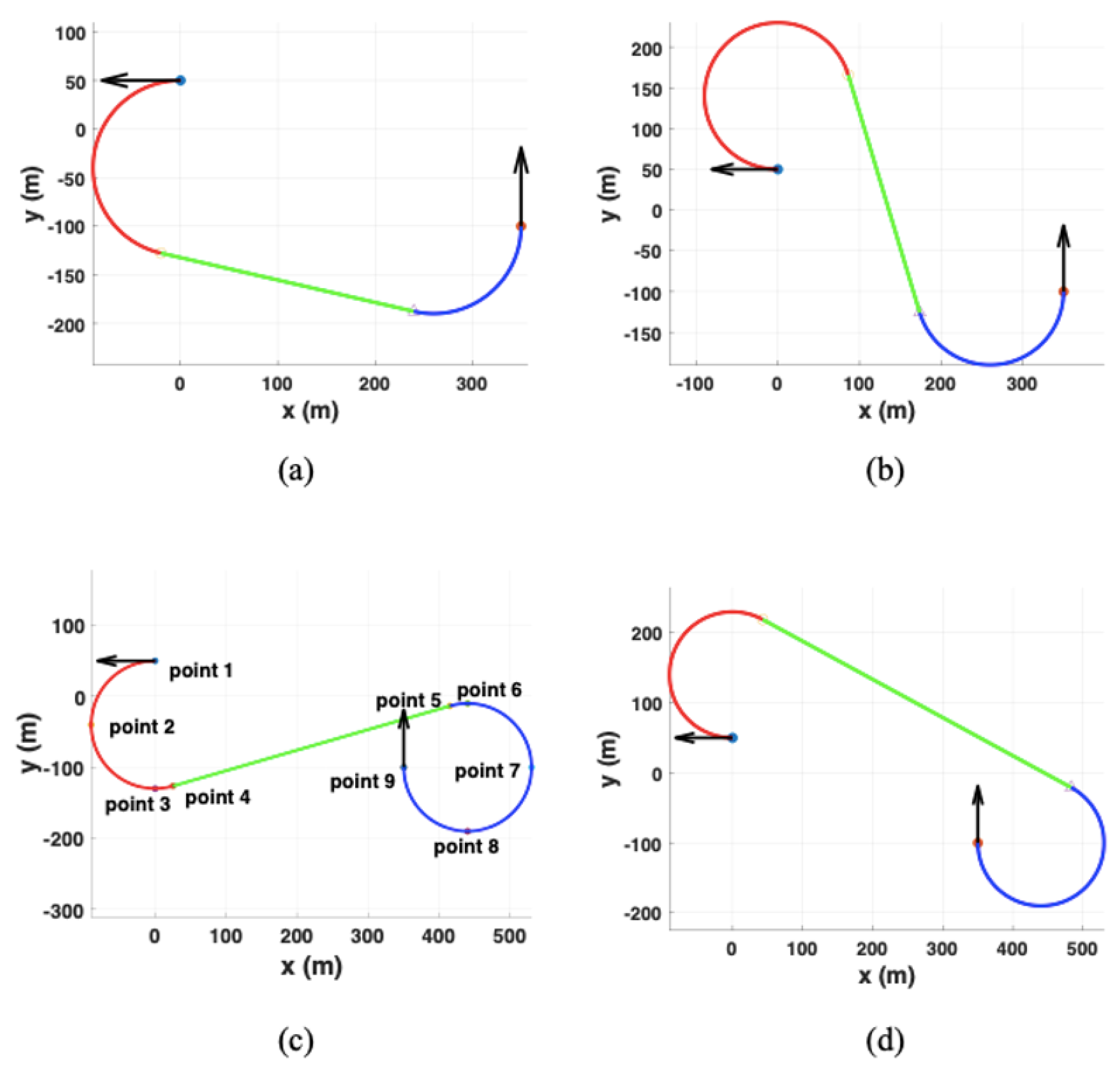Reference [22] has proved that the solution type of Dubins problem in this scenario is CSC. Thus, it is possible to solve the optimal control problem without resorting to inefficient optimal control methods. Instead, the optimal path is obtained by considering only four CSC type paths (LSR, LSL, RSR, RSL). The shortest path is the optimal path. To facilitate real-time path generation, this paper proposes a millisecond-level Dubins path planning method based on analytic geometry. The path generation method is delineated in detail below.

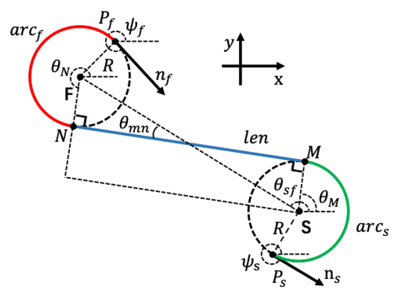
The CSC path consists of three segments: the starting arc $ar{c}_s$, the middle tangent segment $len$, and the ending arc $ar{c}_f$. Four key points exist on the path: the starting point $P_s$, the tangent point M on the starting arc, the tangent point N on the ending arc, and the ending point $P_f$. By identifying these key points, a CSC-type path can be established. Before constructing the path, the 2D Dubins path planning problem is analyzed to gather the necessary known information. These information include the starting point $P_s$, the ending point $P_f$, the turning direction of the starting circle and the ending circle, that is, the left or right turn, and the minimum turning radius R.

First, to obtain the LSR path shown in Figure 5, it is essential to use the turning directions of the starting arc and the ending arc to determine the center S of the starting circle and the center F of the ending circle. This guarantees start arc and end arc position determination. Their coordinates are calculated by

$$(x_S,y_S)=(x_0+R\cos \left({\psi }_0\pm {\displaystyle \frac{\pi }{2}}\right),y_0+R\sin \left({\psi }_0\pm {\displaystyle \frac{\pi }{2}}\right)),$$

(26)

$$(x_F,y_F)=(x_f+R\cos \left({\psi }_f\pm {\displaystyle \frac{\pi }{2}}\right),y_f+R\sin \left({\psi }_f\pm {\displaystyle \frac{\pi }{2}}\right)).$$

(27)

where, when the UAV turns left, the angle is $\psi +\pi /2$; otherwise, the angle is $\psi -\pi /2$.

Then, the coordinates of the tangent points M and N are calculated. According to the coordinates of the centers of the two turning circles, the length of the line $SF$ connecting the centers of the two circles is obtained by

$$le{n}_{SF}=\sqrt{{(y_F-y_S)}^2+{(x_F-x_S)}^2}.$$

(28)

Meanwhile, the angle ${\theta }_{sf}$ between the line $SF$ and the X axis is derived by

$${\theta }_{sf}=\arctan \left({\displaystyle \frac{y_F-y_S}{x_F-x_S}}\right).$$

(29)

From the length of the line segment $SF$ and the radius of the two circles, the angle ${\theta }_{mn}$ between the line $SF$ and the tangent line $MN$ is also gained. When the path type is RSL and LSR, ${\theta }_{mn}$ is calculated by

$${\theta }_{mn}=\arcsin \left({\displaystyle \frac{2R}{le{n}_{SF}}}\right).$$

(30)

When the path type is RSR and LSL, ${\theta }_{mn}$ is obtained from

$${\theta }_{mn}=0.$$

(31)

The position of the tangent point M on the starting circle is determined by the angle ${\theta }_M$ between the line segment $SM$ and the X axis. And ${\theta }_M$ is attained through the geometric relationship with the angle ${\theta }_{sf}$ and the angle ${\theta }_{mn}$, as shown in the

Table 1. The geometric relationship between the definite angle ${\theta }_M$ of the tangent point M and the definite angle ${\theta }_N$ of the tangent point N.

Path Type	${\mathit{\theta }}_{\mathit{M}}$	${\mathit{\theta }}_{\mathit{N}}$
LSL	${\theta }_{sf}-{\theta }_{mn}-\pi /2$	${\theta }_{sf}-{\theta }_{mn}-\pi /2$
LSR	${\theta }_{sf}+{\theta }_{mn}-\pi /2$	${\theta }_{sf}+{\theta }_{mn}+\pi /2$
RSR	${\theta }_{sf}+{\theta }_{mn}-\pi /2$	${\theta }_{sf}+{\theta }_{mn}+\pi /2$
RSL	${\theta }_{sf}-{\theta }_{mn}+\pi /2$	${\theta }_{sf}-{\theta }_{mn}-\pi /2$

. Similarly, the position of the tangent point N on the termination circle can also be determined. The coordinates of the two tangent points are calculated by

$$(x_M,y_M)=\left(x_S+R\cos \left({\theta }_M\right),y_S+R\sin \left({\theta }_M\right)\right),$$

(32)

$$(x_N,y_N)=\left(x_F+R\cos \left({\theta }_N\right),y_F+R\sin \left({\theta }_N\right)\right).$$

(33)

Furthermore, the lengths of the starting arc $ar{c}_s$ and the ending arc $ar{c}_f$ are calculated by

$$le{n}_{ar{c}_s}=R\ast {\theta }_s,le{n}_{ar{c}_f}=R\ast {\theta }_f,$$

(34)

which require the angles ${\theta }_s$ and ${\theta }_f$. The angle ${\theta }_s$ is derived through its geometric relationship with the angle ${\theta }_M$ and the attitude of starting point ${\psi }_s$, as shown in

Table 2. The respective geometric relations of angle ${\theta }_s$ and angle ${\theta }_f$.

Direction	${\mathit{\theta }}_{\mathit{s}}$	${\mathit{\theta }}_{\mathit{f}}$
Left	${\theta }_M-{\psi }_s+\pi /2$	${\psi }_F-{\theta }_N+\pi /2$
Right	${\psi }_s-{\theta }_M+\pi /2$	${\theta }_N-{\psi }_F+\pi /2$

. Similarly, the angle ${\theta }_f$ of the ending arc $ar{c}_f$ is gained through the angle ${\theta }_N$ and the attitude of the ending point ${\psi }_f$. Additionally, the length of the middle tangent segment $len$ is calculated from the coordinates of the tangent points M and N

$$le{n}_{MN}=\sqrt{{(y_N-y_M)}^2+{(x_N-x_M)}^2}.$$

(35)

Finally, the path can be discretized using an appropriate number of points to visualize the path. The coordinates of each discrete point are determined by the interpolation method. Equations (36) and (37), respectively, represent the points on the starting arc and the ending arc whose angular increments are $\epsilon$ and $\mu$. Equation (38) depicts the points on the tangent segment MN, where the length increment is $\tau$, and $(m,n)$ represents the unit direction vector of the tangent segment. By analyzing the two endpoints, M and N, of the tangent segment, we can determine the unit direction vector (39) for the tangent. The desired path is obtained by connecting the discrete points. The pseudocode for generating the optimal Dubins path is presented in Algorithm 1.

$$(x_{S\epsilon },y_{S\epsilon })=(x_S+R\cos \left({\psi }_0\pm {\displaystyle \frac{\pi }{2}}+\epsilon \right),y_S+R\sin \left({\psi }_0\pm {\displaystyle \frac{\pi }{2}}+\epsilon \right))$$

(36)

$$\left(x_{F\mu },y_{F\mu }\right)=(x_F+R\cos \left({\psi }_f\pm \frac{\pi }{2}+\mu \right),y_F+R\sin \left({\psi }_F\pm \frac{\pi }{2}+\mu \right))$$

(37)

$$(x_{len\tau },y_{len\tau })=(x_M+m\tau ,y_M+n\tau )$$

(38)

$$m=(x_N-x_M)/le{n}_{MN},n=(y_N-y_M)/le{n}_{MN}$$

(39)

Algorithm 1: CSC-type Dubins path generation

Input: ${\mathit{P}}_{\mathit{s}}$,${\mathit{P}}_{\mathit{f}}$,$\mathit{R}$

Output: ${\mathit{arc}}_{\mathit{s}}$,${\mathit{arc}}_{\mathit{f}}$,$\mathit{len}$

1: for i = 1:4 do   2:    choose $tur{n}_s$, $tur{n}_f$   3:    calculate $S(x_S,y_S)$ and $F(x_F,y_F)$   4:    determine the tangent points $M(x_M,y_M)$ and $N(x_N,y_N)$   5:    obtain the length of $ar{c}_s$, $ar{c}_f$, $len$   6: the optimal path ← minimum length$\{LSL,LSR,RSR,RSL\}$

4.4. Obstacle Avoidance Strategy in Special Situations

During flight, a UAV swarm frequently encounters no-fly zones, including mountain peaks or areas covered by air defense radar. Consequently, obstacle avoidance becomes an important part of formation flight. The proposed computationally lightweight path generation method offers significant potential in formation obstacle avoidance, as it utilizes the simplified Dubins model suitable for fixed-wing UAVs. A simple example of two-dimensional circular obstacle avoidance is provided for illustration. In this instance, a specific scenario is considered where the planned path not only avoids obstacles for a single UAV, but also for the entire UAV swarm.

The obstacle avoidance problem is also two-dimensional, and the problem scenario is illustrated in Figure 6. It is assumed that the two known static obstacles ${OBS}_1$ and ${OBS}_2$ are of a circular shape. The location of the centers $C_1$ and $C_2$ are $(x_{c1},y_{c1})$ and $(x_{c2},y_{c2})$, respectively, and their radii are $R_1$ and $R_2$ respectively $(R_1\ne R_2)$. A UAV with a specific heading starts from the starting point A, avoids two obstacles, and safely reaches the desired target B with another specific heading. The dotted line ${\mathsf{\Gamma }}_1$ in Figure 6 indicates the path taken by the UAV towards the desired destination point.

The obstacle avoidance path planning method initially assumes an obstacle-free environment and utilizes the previously proposed fast path planning method to generate possible paths from the starting point to the end point. Afterwards, the planned paths need to be assessed for potential intersections with known obstacles. The Dubins path consists of three segments: the initial arc, the middle tangent segment, and the final arc. Therefore, each of the three segments needs to be independently checked against every obstacle to determine if there are any intersections. Whether the starting arc intersects with the obstacle can be determined based on the positional relationship between the starting circle and obstacle circle. Similarly, it can be determined whether the final arc intersects with the obstacle. Whether the middle tangent segment intersects with the obstacle can be determined by the positional relationship between the circle and the straight line. The dotted line ${\mathsf{\Gamma }}_2$ in Figure 6 indicates that the planned path intersects with an obstacle.

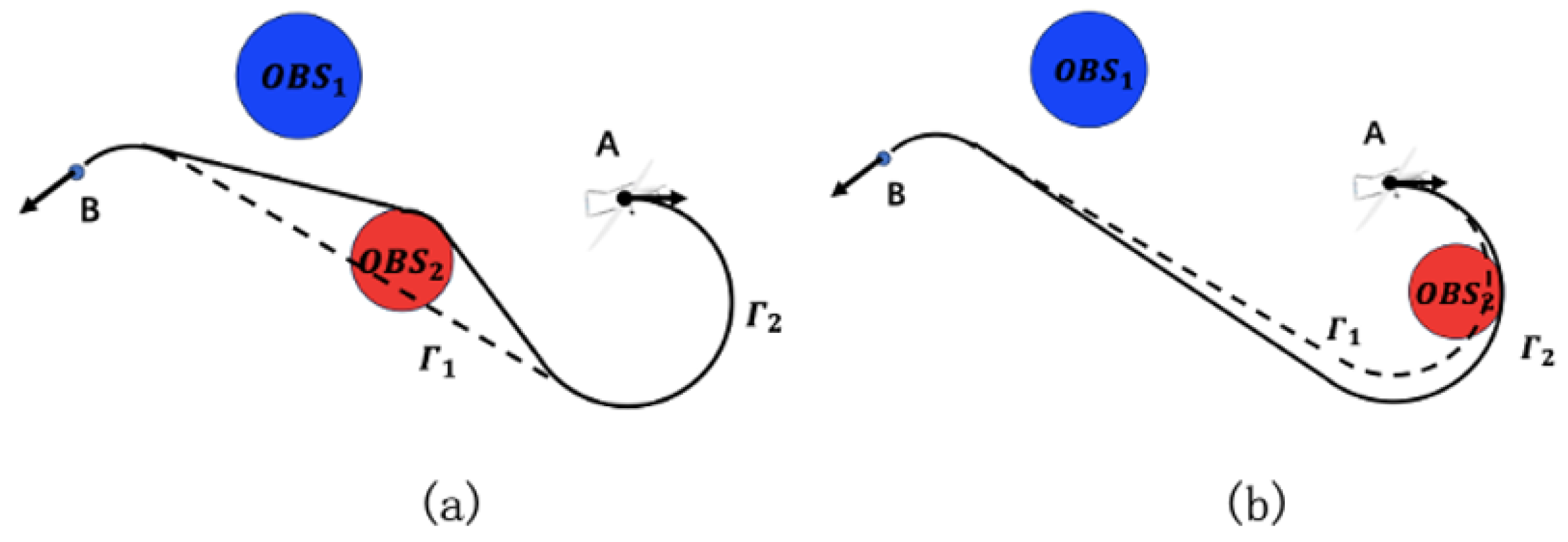
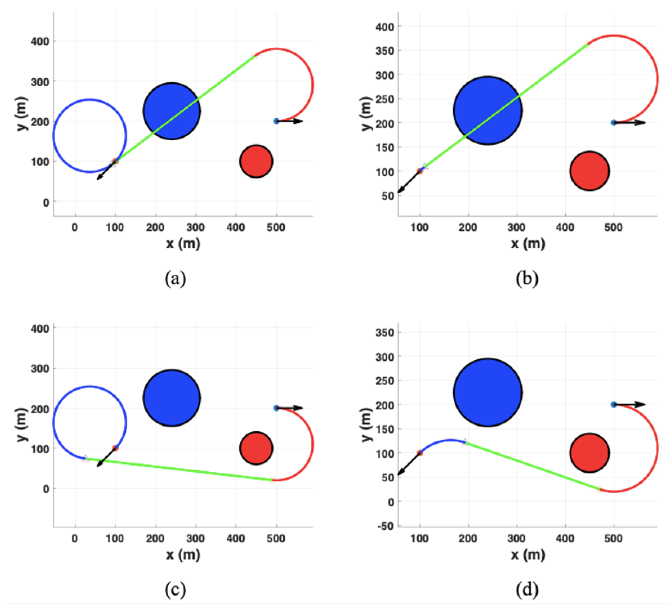
The planned path is deemed feasible if it successfully avoids obstacles. If none of the candidate paths succeed in avoiding obstacles, it becomes necessary to re-plan the path. When the middle tangent segment intersects with the obstacle, the obstacle can be circumvented by adjusting the initial arc and the final arc to make the tangent segment tangential to the obstacle. The final path can thus be viewed as a combination of the two CSC-type Dubins paths. That is, a Dubins path exists between the starting point and the obstacle, and another Dubins path exists between the obstacle and the ending point. In Figure 7a, the middle tangent segment of the path ${\mathsf{\Gamma }}_1$, represented by the dotted line, intersects with the obstacle. In contrast, the path ${\mathsf{\Gamma }}_2$ indicated by the solid line represents the feasible path obtained through the obstacle avoidance method. If the starting arc intersects with an obstacle, then the turning radius of the starting arc is increased in order to inscribe the obstacle and avoid it. The final arc that avoids obstacles can be obtained in the same manner. As shown in Figure 7b, the starting arc of the path ${\mathsf{\Gamma }}_1$, represented by the dotted line, intersects with obstacles, whereas the path ${\mathsf{\Gamma }}_2$ indicated by the solid line is a feasible path obtained by increasing the turning radius. Note that, in practical planning, it is common to maintain a certain distance between the path and the obstacle to ensure safety, rather than achieve exact tangency.

5. Simulation Results and Discussions

In this section, several numerical examples are provided to verify the theoretical results and highlight the applications of the work. First, the reliability of the formation control method is validated. Then, two cases with different complexity examine the viability of the developed path planning method. Furthermore, an example of simple path obstacle avoidance in a special case demonstrates the application potential of the path planning method. Finally, a performance comparison of relevant methods and the scalability of the proposed method are discussed.

5.1. Formation Control Simulation

The formation control method not only controls the chaotic UAV swarm into the desired UAV formation, but also plays a prominent role in maintaining the geometric characteristics of the formation during the formation path flight. In addition, during subsequent large-scale formation path flight simulations, the initial position and attitude of the UAV swarm are similar to the nominal formation, enabling a shorter formation maneuver time. Thus, it is essential to ensure that the method can form the desired UAV formation from an arbitrary initial state of UAV swarms.

Given a nominal formation of six fixed-wing UAVs, its corresponding undirected graph is shown in Figure 8a. The distance between any two connected UAVs in the formation is maintained at 10 m. The minimum speed of the UAV is set at $v_{min}=3$ m/s, while the maximum speed is $v_{max}=5$ m/s, and the maximum angular speed is ${\omega }_{max}=(\pi /4)$ rad/s. The simulation utilizes the fixed-wing UAV model presented in (1) and (9), along with the corresponding control law (5) and (6). In this formation control simulation, the initial position and initial attitude of the UAV are given arbitrarily, as shown in Figure 9a. The effects of measurement errors or noise on formation control are not considered. Figure 9b–d display the status of the UAV formation at different times. As seen from Figure 9, the hybrid formation control method can effectively form the UAV swarm in the chaotic initial state into the desired formation within a brief period.

5.2. Path Planning Flight Simulation

To validate the effectiveness of the fast path planning framework for large-scale fixed-wing UAV formations, two different simulations with desired formations defined as a triangle are performed. Given a nominal formation of 16 fixed-wing UAVs, its undirected graph is shown in Figure 8b. The nominal distance between UAVs inside the formation is 40 m, and the nominal distance between UAVs on the formation boundary is $40\sqrt{2}$ m. The minimum speed of the UAV is $v_{min}=8$ m/s, the maximum speed is $v_{max}=15$ m/s, and the maximum angular speed is ${\omega }_{max}=(\pi /35)$ rad/s. When the formation control is completed, the expected motion direction of the UAV formation is $\psi =\pi$.

Example 1: In the first example, the states of the starting and ending points are $(0,0,\pi )$ and $(380,0,\pi )$, respectively. The extreme value of the control variable is $1/90$. Note that the unit of the location and length is in meters, and the unit of heading angle is in radians. The generation of Dubins path are realized on the Intel Core 1.6 GHz laptop with 8 GB RAM. The problem-solving time is 3.1 ms, and the four CSC-type paths are shown in Figure 10. Figure 10a,b show the optimal solution among given orientation points, LSL and RSR. Due to the particularity of the initial state and the terminal state, the two different types of paths are symmetrical, and the path length is 945.4867. Similarly, this example has two symmetric, stable suboptimal solutions, RSL and LSR, as shown in Figure 10c,d, respectively. The total path length is 1104.7414.

In the flight simulation, the initial positions and attitudes of the 16 UAVs are selected arbitrarily. However, due to the large number of UAVs and the large minimum radius of curvature, the formation maneuvering takes long time. For the purpose of shortening the time of formation maneuvering as much as possible, the initial positions of all UAVs are chosen near the nominal position. Figure 11a shows the initial state of the UAV formation. The optimal RSR-type path, referred to as Path 1, is selected as the target path. The path is discretized by six waypoints, as shown in the Figure 10b. The purpose of setting waypoints is to measure the error in formation maintenance. Figure 11b illustrates that the UAV formation adopts the hybrid control law to achieve a nominal formation.

Figure 12a supplements the variation of distance errors between UAVs at different positions during formation control. The distance error between UAVs is calculated based on the actual and nominal distances. Two pairs of UAVs are selected from both the boundary and the interior of the formation, respectively. The distance error between UAVs at different locations exhibits significant variation. However, after a period of maneuvering, the distance error is controlled within an acceptable range. The variation of heading angle errors of the UAVs at different positions is presented in Figure 12b. The heading error of the UAV is calculated by the difference between its actual heading angle and the expected heading angle of the formation. The control of heading angle error is rapidly achieved, enabling the UAV to navigate towards the desired heading after a short period of control. Once the formation control is accomplished, the formation achieves the required geometric characteristics, such as shape, distance, and direction. Four frames are extracted from the trajectory of the UAV formation flying the Dubins path in Figure 11c–f. As shown, the UAV formation can perfectly fly the planned path while maintaining the geometric characteristics of the formation. The position errors of UAVs at different positions passing through each waypoint during formation flight are shown in

Table 3. Position error of waypoints on path 1 of UAVs at different positions.

Waypoint	2	3	4	5	6
UAV1 Position error (m)	0.97	2.38	2.82	0.51	0.14
UAV7 Position error (m)	1.34	1.97	1.98	0.96	0.77
UAV10 Position error (m)	2.20	2.98	2.03	1.00	0.71
UAV16 Position error (m)	1.54	1.77	1.56	1.27	1.40

. UAVs at various positions in the formation have different linear position errors through the same waypoint, yet waypoints with large position errors tend to be similar. Figure 13a displays the distance error between UAVs at different positions during the UAV formation flight along the planned path, with errors remaining within the acceptable range. Video of simulation is available in Supplementary Materials.

Example 2: The second example is a path with two different long arcs. Compared with example 1, the distance between two orientation points in example 2 is larger, the attitude changes are larger, and the forms of solutions are more diverse. The states of the starting and ending points are $(0,50,\pi )$ and $(350,-100,\pi /2)$. The extreme value of the control variable is $1/90$. The problem-solving time is 3.73 milliseconds, and the four CSC-type paths are shown in Figure 14. Example 2 has four completely different paths, and the optimal path is LSL, as shown in Figure 14a. Figure 14b–d are other stable solutions, RSL, LSR, and RSR, respectively. From the figure, it is evident that the length of the optimal path is only half that of the longest path. Moreover, the optimal path is simpler and has shorter arcs.

In the flight simulation of example 2, the optimal path is not selected. Instead, a more intricate LSR-type path called Path 2 is chosen. The purpose of choosing a suboptimal path is to demonstrate the ability of fixed-wing UAVs to fly more complex paths. Nine representative waypoints are selected on the path, as shown in the Figure 14c. In the flight simulation of example 2, the initial state of UAVs matches that of Example 1. As a result, the initial state of the UAV formation in example 2, as well as the nominal formation achieved after the formation control, correspond to those depicted in Figure 11a,b. In Figure 15a–f, six frames are extracted from the trajectory of the UAV formation flying the Dubins path. These frames illustrate that UAV formation can fly more complex paths. Figure 13b shows the distance error between the UAVs at different positions during the UAV formation’s navigation along the planned path, with errors remaining within the acceptable range.

Table 4. Position error of waypoints on path 2 of UAVs at different positions.

Waypoint	2	3	4	5	6	7	8	9
UAV1 Position error (m)	0.49	2.07	2.40	2.73	2.21	1.19	3.97	0.96
UAV7 Position error (m)	0.37	2.28	2.63	2.82	2.35	1.20	4.11	1.00
UAV10 Position error (m)	1.16	1.40	2.28	3.30	2.04	2.09	3.85	0.27
UAV16 Position error (m)	0.38	2.29	2.65	2.76	2.50	1.03	4.21	1.24

details the position error of the UAVs at different positions in the formation passing through the waypoint during the formation flight. Compared with example 1, example 2 exhibits not only a larger maximum position error, but also increased errors at each waypoint. These phenomena result from two factors. On the one hand, the path of example 2 is longer and more complicated, which will increase the cumulative error. On the other hand, the path of example 2 features a long arc path, leading to increased error in tracking the path while maintaining the geometric characteristics of the formation. Video of simulation is available in Supplementary Materials.

5.3. Formation Obstacle Avoidance Simulation

The states of the starting and ending points are $(500,200,0)$ and $(100,100,5\pi /4)$, respectively, and the extreme value of the control variable is $1/90$. Circles in various colors depict obstacles, with radii of 40 m and 70 m, located at $(450,100)$ and $(240,225)$, respectively. The four CSC paths are shown in Figure 16. Upon collision assessment, both the LSL and LSR paths intersect through obstacles, whereas the RSL and RSR paths avoid obstacles to reach their destinations. The RSL path is not only the shortest, but is also a safe path for avoiding obstacles.

The obstacle avoidance flight simulation involves 10 fixed-wing UAVs arranged in a desired triangular formation, with the formation’s shape shown in Figure 17a. The distance between any two UAVs in the formation is 20 m, and the expected motion direction of the UAV formation is $\psi =0$ when the formation control is completed. The minimum velocity of the UAV in the formation is $v_{min}=8$ m/s, the maximum velocity is $v_{min}=10$ m/s, and the maximum angular velocity is ${\omega }_{max}=(\pi /33.2)$ rad/s. Rather than detailing the state of the UAV swarm during the formation control stage, a schematic representation of the UAV swarm’s obstacle avoidance behavior is provided in detail in Figure 17 for a more concise presentation. Figure 17a–f illustrate the trajectory of the UAV swarm during obstacle avoidance, successfully avoiding two obstacles. For simplicity, the relevant distance error figures have been omitted. These results highlight the potential application of the proposed path planning method for obstacle avoidance in large-scale, simple formations. Video of simulation is available in Supplementary Materials.

5.4. Performances Comparison

To obtain a clear understanding of the features and advantages of the proposed method over the widely used formation path planning methods, a summary is compiled from [24,25], highlighting key performance metrics for comparison in

Table 5. Performance comparison of formation path planning methods: Fast (FS), Formation Maintenance (FM), Optimal (OP), Internal Collision Avoidance (ICA). ✔ indicates that the method performs well in terms of performance, while ✘ indicates that the method performs poorly in terms of performance improvement.

Formation Path Planning Method	FS	FM	OP	ICA
Potential Fields [26,27]	✔	✘	✘	✔
Optimization-Based [8]	✘	✘	✔	✔
Intelligent Evolution-Based [9]	✘	✘	✘	✔
Ours	✔	✔	✔	✔

. The focus is on the following aspects: formation assembly, formation maintenance, fast planning, optimality, and internal collision avoidance. Fast planning enables real-time online path planning for UAVs, which is of great significance for obstacle avoidance. Formation maintenance ensures that the UAV formation consistently maintains the desired shape, distances, and angles during flight, allowing the UAV swarm to move as a single rigid body. As a system with limited energy, fixed-wing UAV benefits from the shortest path, which aids in reducing energy consumption and quickly reaching the target. Collision avoidance within the UAV formation guarantees that there are no collisions between UAVs during flight, which is essential for safe formation flight. It can be seen that the proposed method excels in the properties of interest. Compared to previous methods, it is more comprehensive. Note that the existing literature on formation path planning rarely provides the corresponding method planning path time, making a detailed comparison challenging. Hence, the relevant performance of single UAV path planning is used to qualitatively evaluate the planning speed.

5.5. Scalability of Methods

Prior to specific path generation, regardless of the number of UAVs in the formation and their initial positions, the UAV swarm forms the desired formation under the control of the formation control strategy, moving as a single rigid body. Therefore, the path generation targets the entire UAV formation, and the formation’s path can be obtained with just one path planning. The path planning time of the proposed method is independent of both the formation size and initial position, and it is in the order of milliseconds for formations of any scale. Whether the proposed method can be applied to larger formations depends on if the formation control method can accomplish the task of formation control. In Section 4, the formation control method’s validity is demonstrated using the Lyapunov stability theorem. The proof places no restrictions on the formation scale and initial position; in other words, the formation control method is capable of handling formations of any initial position and any size. Hence, the proposed method is scalable to larger-scale UAV formations.

In the previously mentioned three types of simulations, there are formations containing different numbers of UAVs: a 6-unit formation for formation control simulation, a 10-unit formation for formation obstacle avoidance simulation, and a 16-unit formation for formation path planning. These indicate that the proposed method possesses scalability. To effectively apply the proposed method to larger formations, it is essential to determine the information required for formation control and the corresponding control matrix. Firstly, the formation’s composition should be provided, including the number of UAVs in the formation and an undirected graph depicting the communication relationships among the UAVs. Subsequently, the shape of the UAV formation, as well as the spacing and angle between individual UAVs, needs to be specified. Finally, the control gain matrix and distance control matrix should be determined using the method introduced in Section 4. The desired formation can be formed utilizing the formation control law.

6. Conclusions

This paper proposes a fast path planning framework for large-scale distributed fixed-wing UAV formations. This path planning method is implemented on the premise that the UAV swarm forms the desired formation. The formation control method first forms the UAV swarm in any initial state into desired formation, which will also play a role in maintaining the geometric characteristics and avoiding internal collisions during the formation flight. A UAV swarm that has completed formation control can be regarded as a large fixed-wing UAV, allowing a single path planning to generate a feasible path for the entire formation. Given the need for a real-time solution for path planning in fixed-altitude flight, this paper adopts the Dubins path generation method. Based on analytic geometry, it forms an integral part of the overall method, aiming to obtain the optimal path under specific conditions. Additionally, brief introductions are provided on obstacle avoidance strategies for specific scenarios, showcasing potential applications of the proposed method.

The simulation of formation control confirms the capability of the hybrid control method employed to form the desired fixed-wing UAV formation from any disordered initial position. Two different formation path planning scenarios and their simulated flights illustrate the effectiveness of the proposed fast path planning framework, obtaining a feasible path for the entire formation with just one millisecond-level path planning. Moreover, the UAV formation is not only able to perfectly maintain the formation’s geometric characteristics but also effectively avoid collisions among UAVs during the flight. A simple case of formation obstacle avoidance demonstrates that the proposed path planning method is applicable to formation obstacle avoidance. Simulation experiments involving formations of different scales further demonstrate the scalability of the proposed method. While the proposed method excels in rapid path planning and maintaining formation characteristics, it possesses limitations that necessitate future research. Although path planning time does not significantly increase with a greater number of agents, the complexity and time needed for formation control do increase. This calls for more advanced formation control methods. Moreover, in contemplating deployment on UAV systems, upcoming studies will tackle formation challenges in real-world settings, including 3D path planning, general obstacle avoidance, and measurement noise.

References

1. Rudol, P.; Doherty, P. Human Body Detection and Geolocalization for UAV Search and Rescue Missions Using Color and Thermal Imagery. In Proceedings of the IEEE Aerospace Conference, Big Sky, MT, USA, 1–8 March 2008; pp. 1–8. [Google Scholar]
2. Goodrich, M.A.; Morse, B.S.; Gerhardt, D.; Cooper, J.L.; Quigley, M.; Adams, J.A.; Humphrey, C. Supporting wilderness search and rescue using a camera-equipped mini UAV. J. Field Robot. 2008, 25, 89–110. [Google Scholar] [CrossRef]
3. Zhang, J.; Hu, J.; Lian, J.; Fan, Z.; Ouyang, X.; Ye, W. Seeing the forest from drones: Testing the potential of lightweight drones as a tool for long-term forest monitoring. Biol. Conserv. 2016, 198, 60–69. [Google Scholar] [CrossRef]
4. Scherer, J.; Rinner, B. Persistent multi-UAV surveillance with energy and communication constraints. In Proceedings of the 2016 IEEE International Conference on Automation Science and Engineering (CASE), Fort Worth, TX, USA, 21–25 August 2016; pp. 1225–1230. [Google Scholar]
5. Anderson, B.D.O.; Fidan, B.; Yu, C.; Walle, D. UAV formation control: Theory and application. In Recent Advances in Learning and Control; Springer: London, UK, 2008; pp. 15–33. [Google Scholar]
6. Zhou, W.; Chen, H.; Li, J.; Chen, Y. Formation Trajectory Planning of Fixed-Wing UAV Swarms. In Proceedings of the 2021 5th Chinese Conference on Swarm Intelligence and Cooperative Control, Shenzhen, China, 19–22 January 2021; Springer: Singapore, 2022; pp. 1650–1662. [Google Scholar]
7. Zhang, M.; Liu, C.; Wang, P.; Yu, J.; Yuan, Q. UAV swarm real-time path planning algorithm based on improved artificial potential field method. In Proceedings of the 2021 International Conference on Autonomous Unmanned Systems (ICAUS 2021), Changsha, China, 24–26 September 2021; Springer: Singapore, 2022; pp. 1933–1945. [Google Scholar]
8. Wang, W.; Wang, M.; Qi, J.; Wu, C.; Liu, Z. Motion Planning for Fixed-Wing UAV Formations Flight With Velocity and Heading Rate Constraints. In Proceedings of the 2022 41st Chinese Control Conference (CCC), Hefei, China, 25–27 July 2022; pp. 3761–3767. [Google Scholar]
9. Shao, S.; Peng, Y.; He, C.; Du, Y. Efficient path planning for UAV formation via comprehensively improved particle swarm optimization. ISA Trans. 2020, 97, 415–430. [Google Scholar] [CrossRef] [PubMed]
10. Deghat, M.; Anderson, B.D.O.; Lin, Z. Combined flocking and distance-based shape control of multi-agent formations. IEEE Trans. Autom. Control 2015, 61, 1824–1837. [Google Scholar] [CrossRef]
11. Han, T.; Lin, Z.; Zheng, R.; Fu, M. A barycentric coordinate-based approach to formation control under directed and switching sensing graphs. IEEE Trans. Cybern. 2017, 48, 1202–1215. [Google Scholar] [CrossRef]
12. Trinh, M.H.; Zhao, S.; Sun, Z.; Zelazo, D.; Anderson, B.D.O.; Ahn, H.S. Bearing-based formation control of a group of agents with leader-first follower structure. IEEE Trans. Autom. Control 2018, 64, 598–613. [Google Scholar] [CrossRef]
13. Fathian, K.; Rachinskii, D.I.; Summers, T.H.; Spong, M.W.; Gans, N.R. Distributed formation control under arbitrarily changing topology. In Proceedings of the 2017 American Control Conference (ACC), Seattle, WA, USA, 24–26 May 2017; pp. 271–278. [Google Scholar]
14. Fathian, K.; Summers, T.H.; Gans, N.R. Distributed formation control and navigation of fixed-wing UAVs at constant altitude. In Proceedings of the 2018 International Conference on Unmanned Aircraft Systems (ICUAS), Dallas, TX, USA, 12–15 June 2018; pp. 300–307. [Google Scholar]
15. Kaminer, I.; Yakimenko, O.; Pascoal, A.; Ghabcheloo, R. Path generation, path following and coordinated control for timecritical missions of multiple UAVs. In Proceedings of the 2006 American Control Conference, Minneapolis, MN, USA, 14–16 June 2006; pp. 4906–4913. [Google Scholar]
16. Choe, R.; Cichella, V.; Xargay, E.; Hovakimyan, N.; Trujillo, A.C.; Kaminer, I. A trajectory-generation framework for time-critical cooperative missions. In Proceedings of the AIAA Infotech@Aerospace (I@A) Conference, Boston, MA, USA, 19–22 August 2013; p. 4582. [Google Scholar]
17. Gao, C.; Gong, H.; Zhen, Z.; Zhao, Q.; Sun, Y. Three dimensions formation flight path planning under radar threatening environment. In Proceedings of the 33rd Chinese Control Conference, Nanjing, China, 28–30 July 2014; pp. 1121–1125. [Google Scholar]
18. Blasi, L.; D’Amato, E.; Notaro, I.; Raspaolo, G. Clothoid-Based Path Planning for a Formation of Fixed-Wing UAVs. Electronics 2023, 12, 2204. [Google Scholar] [CrossRef]
19. Arani, A.H.; Azari, M.M.; Melek, W.; Safavi-Naeini, S. Learning in the sky: Towards efficient 3D placement of UAVs. In Proceedings of the IEEE 31st Annual International Symposium on Personal, Indoor and Mobile Radio Communications, London, UK, 31 August–3 September 2020; pp. 1–7. [Google Scholar]
20. Consonni, C.; Brugnara, M.; Bevilacqua, P.; Tagliaferri, A.; Frego, M. A new Markov–Dubins hybrid solver with learned decision trees. Eng. Appl. Artif. Intell 2023, 122, 106166. [Google Scholar] [CrossRef]
21. Dubins, L.E. On curves of minimal length with a constraint on average curvature, and with prescribed initial and terminal positions and tangents. Am. J. Math 1957, 79, 497–516. [Google Scholar] [CrossRef]
22. Hota, S.; Ghose, D. Optimal path planning for an aerial vehicle in 3D space. In Proceedings of the 49th IEEE Conference on Decision and Control (CDC), Atlanta, GA, USA, 15–17 December 2010; pp. 4902–4907. [Google Scholar]
23. Kaya, C.Y. Markov–Dubins path via optimal control theory. Comput. Optim. Appl. 2017, 68, 719–747. [Google Scholar] [CrossRef]
24. Subies Hueso, J.; Mondal, S.; Tsourdos, A.; Chadwick, A. Real-Time Collision Avoidance Trajectory Planner Using Generalized Vector Explicit Guidance. In Proceedings of the AIAA SCITECH 2023 Forum, National Harbor, MD, USA & Online, 23–27 January 2023; p. 1734. [Google Scholar]
25. Yasin, J.N.; Mohamed, S.A.S.; Haghbayan, M.H.; Heikkonen, J.; Tenhunen, H.; Plosila, J. Unmanned aerial vehicles (uavs): Collision avoidance systems and approaches. IEEE Access 2020, 8, 105139–105155. [Google Scholar] [CrossRef]
26. Benghezal, A.; Louali, R.; Bazoula, A.; Chettibi, T. Path planning of fixed wing UAVs formation. In Proceedings of the 2015 First International Conference on New Technologies of Information and Communication (NTIC), Mila, Algeria, 8–9 November 2015; pp. 1–7. [Google Scholar]
27. Fang, Y.; Yao, Y.; Zhu, F.; Chen, K. Piecewise-potential-field-based path planning method for fixed-wing UAV formation. Sci. Rep. 2023, 13, 22–34. [Google Scholar] [CrossRef] [PubMed]
Figure 1. Schematic of the path planning method for large-scale distributed fixed-wing UAV formation.
Aerospace 11 00001 g001
Figure 2. Schematic of fixed-wing UAV formation.
Aerospace 11 00001 g002
Figure 3. Formation path planning scenario.
Aerospace 11 00001 g003
Figure 4. Geometry of the Dubins problem.
Aerospace 11 00001 g004
Figure 5. Geometric intuition of CSC-type path construction. Green arc represents the starting arc, blue line represents the middle tangent segment, and red arc represents the ending arc.
Aerospace 11 00001 g005
Figure 6. Obstacle avoidance scenario.
Aerospace 11 00001 g006
Figure 7. Geometric intuition of path re-planning in different cases. (a) Obstacle avoidance path when the tangent segment intersects with obstacles. (b) Obstacle avoidance path when the starting arc intersects with obstacle.
Aerospace 11 00001 g007
Figure 8. Schematic of the nominal formation of fixed-wing UAVs. (a) The nominal formation of 6 fixed-wing UAVs in the formation control simulation. (b) The nominal formation of 16 fixed-wing UAVs in the formation flight simulation.
Aerospace 11 00001 g008
Figure 9. Simulation experiment of formation control method. (a) Any given initial position of UAV swarm. (bd) State of UAV formation at different times. Different colors represent the trajectories of different UAVs.
Aerospace 11 00001 g009
Figure 10. Solution of path planning example 1. (ab) The optimal solution between the given orientation points, t f = 945.4867 . (cd) The other stable solutions between the same orientation points, t f = 1104.7414 . Red arc represents the starting arc, green line represents the middle tangent segment, and blue arc represents the ending arc.
Aerospace 11 00001 g010
Figure 11. The fixed-wing UAV formation completes the formation maneuver from any initial position to form a nominal formation, and then flies according to the planned path. (af) represent the status of the UAV formation at different times. Different colors represent the trajectories of different UAVs.
Aerospace 11 00001 g011
Figure 12. UAVs’ distance and angle error versus time during formation control. (a) Distance error between UAVs, where e i j is the distance error between UAV i and UAV j. (b) Angle error, where e k is the error between the actual heading angle of UAV k and the desired heading angle.
Aerospace 11 00001 g012
Figure 13. The distance error between UAVs during the formation flight. (a) UAV distance error in example 1, where e i j is the error between UAV i and UAV j. (b) UAV distance error in example 2, where e i j is the error between UAV i and UAV j.
Aerospace 11 00001 g013
Figure 14. Solution of path planning example 2. (a) Optimal solution between the given orientation points, t f = 690.9483 . (bd) Suboptimal solution between the same orientation points, t f = 958.9849 , t f = 1163.5421 , t f = 1208.0569 . Red arc represents the starting arc, green line represents the middle tangent segment, and blue arc represents the ending arc.
Aerospace 11 00001 g014
Figure 15. Fixed-wing UAV formation flight LSR Dubins path. (af) represent the state of UAV formation at different time points. Different colors represent the trajectories of different UAVs.
Aerospace 11 00001 g015
Figure 16. Formation obstacle avoidance path planning. (ab) LSR and LSL path through obstacles. (cd) RSL path and RSR path to avoid obstacles. Red arc represents the starting arc, green line represents the middle tangent segment, and blue arc represents the ending arc. Circles of different colors represent different obstacles.
Aerospace 11 00001 g016
Figure 17. Schematic of obstacle avoidance flight of fixed wing UAV formation. (af) represent the state of UAV formation at different time points. Different colors represent the trajectories of different UAVs.
Aerospace 11 00001 g017