Article

Influence of Engine Dynamic Characteristics on Helicopter Handling Quality in Hover and Low-Speed Forward Flight

1
National Key Laboratory of Helicopter Aeromechanics, College of Aerospace Engineering, Nanjing University of Aeronautics and Astronautics, Nanjing 210016, China
2
Department of Aerospace Engineering, Swansea University, Swansea SA1 8EN, UK
*
Author to whom correspondence should be addressed.
Aerospace 2024, 11(1), 34; https://doi.org/10.3390/aerospace11010034
Submission received: 31 October 2023 / Revised: 26 December 2023 / Accepted: 27 December 2023 / Published: 29 December 2023
(This article belongs to the Section Aeronautics)

Abstract

:
This study assesses the influence of engine dynamic characteristics on helicopter handling quality during hover and low-speed forward flight. First, we construct the helicopter–engine coupling model (HECM) based on the power-matching relationship between the engine and the rotor. The impact of the engine is evaluated by comparing HECM with a helicopter model without the engine. To assess the engine’s influence quantitatively, we consider torque response, height response, and collective–yaw coupling characteristics in ADS-33E-PRF handling quality criteria. The results reveal that the engine power output lag can deteriorate the helicopter’s torque and height response handling quality rate (HQR). After the increase in helicopter mass, the torque HQR caused by engine influence improved, and the altitude HQR further deteriorated. The engine dynamic characteristics can also reverse the yaw rate, decreasing collective–yaw coupling HQR. As the helicopter’s flight speed increased, the engine’s impact on the yaw rate increased by 41.8%. This study can provide valuable insight into the effects of engine dynamic characteristics on helicopter handling quality and offer a reference for the design of helicopter–engine coupling control laws.

1. Introduction

Helicopter handling quality, an essential metric that characterizes the stability and maneuverability of helicopters, plays a pivotal role in the design of both helicopter and control systems. However, due to the complexity of the coupling relationship between the aircraft and the engine, the influence of the engine dynamic characteristics on the helicopter handling quality has not been studied for a long time [1]. Consequently, developing a comprehensive helicopter model capable of elucidating the engine’s dynamic characteristics and quantitatively assessing its impact on helicopter handling quality becomes imperative. This work deepens our understanding of the coupling relationship between the helicopter and the engine and assumes paramount importance in formulating helicopter–engine coupling model (HECM) control algorithms.
The ADS-33E-PRF [2] is the handling qualities specification for military rotorcraft, released in March 2000. Since its inception, researchers have widely adopted this standard to evaluate existing helicopters, design future helicopters, improve the flight control systems installed on existing helicopters, and quantitatively analyze the interference of other factors on helicopters. To evaluate existing helicopters, Celi [3] used inverse simulation methods to evaluate the helicopter’s roll and pitch rate. Luria [4] evaluated the UH-60M fly-by-wire helicopter using standards such as bandwidth and speed. Malpica [5] evaluated the task subject completion of heavy tilt-rotor aircraft in hover and low-speed forward flight under a given response type. At the same time, handling quality standards are also widely used in the design of new helicopters. Lawrence [6] incorporated stability and control analysis into the conceptual design process of helicopters and used handling quality standards to guide the selection of component parameters on helicopters. Gerosa [7] used bandwidth and phase delay to optimize the helicopter design process. Meanwhile, researchers are increasingly using handling quality standards to optimize the parameters of existing helicopter flight control systems. Tischler [8] uses the CONDUIT (control designer’s unified interface) tool to design helicopter flight control systems based on handling quality requirements. Horn [9,10] uses stability margin and bandwidth to evaluate the benefits of helicopter rotor state feedback (RSF) control. Türe [11] optimized the design of helicopter flight control systems based on bandwidth and quickness requirements. In addition, handling quality standards are widely used to evaluate the interference of other factors on helicopters. Ji [12] used a high-precision turbine model to assess the impact of aerodynamic changes in helicopter components in distributed atmospheric turbulence on handling quality. Yuan [13,14] assessed the effect of aerodynamic interference on the handling quality of tractor aircraft using the uncertainty quantification method. Yan [15,16] used the wavelet analysis method to evaluate the pilot load of the XV-15 tiltrotor aircraft in conversion modes. However, there have been relatively few assessments of the impact of engines on the handling quality of helicopters. The coupling relationship between the engine and the aircraft minimally influences their respective operating states during stable flight. Conversely, when the rapid change of helicopter flight state causes the rapid change of the required power signal, the influence of the engine dynamic characteristics on the helicopter handling quality cannot be ignored. Therefore, it is necessary to establish a helicopter flight dynamics model that can accurately reflect the influence of engine dynamic characteristics.
In the past, the complexity of the helicopter engine system often led to their separate modeling, with helicopters and engines considered independent entities. In helicopter design, idealized or simplified engine models have traditionally been employed. Notable examples of such efforts include the ARMCOP (the generic real-time helicopter simulation model developed at Ames Research Center) model developed by Talbot [17,18], Corliss’s research [19] on helicopter NOE (nap-of-the-earth) maneuver, and Cho’s helicopter/power component coupling model [20]. On the other hand, in engine modeling, simplified helicopter models are often used. These endeavors encompass tasks such as assessing the impact of load variations on engine output speed [21] and optimizing engine control system parameters [22,23,24]. It is worth noting that the modeling of the HECM began relatively late, starting in the late 1970s. Richardson [25,26] introduced a helicopter–engine coupling model to address resonance and dynamic stability issues experienced during helicopter flight. Hull [27] summarized prior work in this area and underscored the potential consequences of the coupling between the rotor and the engine, which could result in rapid changes in rotor speed, thereby affecting helicopter flight performance. Mihaloew [28] utilized a helicopter–engine coupling model to enhance engine fuel control by implementing an LQR (linear quadratic regulator) control law and reducing rotor speed variations. However, these studies did not delve into the impact of torque and speed changes on helicopter handling quality. With the development of rotor variable speed technology, Han et al. [29,30,31,32,33] developed the helicopter–engine coupling model to analyze helicopter performance following changes in rotor speed. They aimed to determine the optimal rotor speed by minimum power and fuel flow consumption. However, most of these studies predominantly concentrated on the steady-state operational characteristics of engines without an in-depth analysis of the potential influence of engine dynamic characteristics on helicopter handling quality.
In light of the preceding discussion, this article analyzes the engine dynamic characteristics affecting helicopter handling quality by developing a helicopter–engine coupling model. The content of this article is arranged as shown in Figure 1. First, the helicopter flight dynamics model with rotor, tail rotor, and other parts is established. Second, we establish the engine aerodynamic thermodynamic model based on the part model of the compressor, gas turbine, power turbine, and other components. Then, HECM is formulated based on the power-matching relationship between the rotor and the engine. Finally, based on the torque, altitude, and collective–yaw coupling handling quality characteristics in ADS-33E-PRF, we compare the handling quality calculation results of helicopter models with and without engine modules and quantitatively analyze the impact of engine dynamic characteristics on helicopter handling quality.

2. Mathematical Model

2.1. Helicopter Model

The helicopter flight dynamics model is established using UH-60A as the sample reference model [34,35,36]. The helicopter is divided into five major parts: the main rotor, tail rotor, fuselage, vertical tail, and horizontal tail.
The main rotor model is constructed using the blade element method rather than the traditional rotor disk model. This choice is motivated by the need to accurately simulate the rotor dynamic response when the rotor speed changes. Rotor speed and its derivatives are input from the engine model. Changes in rotor speed can result in variations in blade element incoming velocity, leading to alternations in blade flap and lead–lag motion, and finally affect the rotor forces and moments.
The rotor blade flap and lead–lag motion are computed using the global Galerkin method. The global Galerkin method is the same as the harmonic balance method, which treats flap and lag motion as a Fourier series, and the frequency is the same as rotor speed. Using flap motion as an example, the derivative of the flap motion over time provides the flap rate and flap acceleration approximation (denoted as β ¨ a p p ). By applying the moment balance equation of the flap motion, flap acceleration (denoted as β ¨ ) can be calculated. The global Galerkin method accounts for the rotor trim when the coefficients of the flap acceleration approximation series β ¨ a p p coincide with flap acceleration β ¨ on average. The trim equation of the global Galerkin method on the flap is shown below [37]:
0 2 π ( β ¨ β ¨ a p p ) d ψ = 0 0 2 π ( β ¨ β ¨ a p p ) sin k ψ d ψ = 0 0 2 π ( β ¨ β ¨ a p p ) cos k ψ d ψ = 0 ,
in which ψ is the blade azimuth angle; and k is the harmonic order of the flap Fourier series. The lead–lag motion is calculated in the same way.
Changes in the flapping and lead–lag motions of the blades will cause changes in the rotor aerodynamic force, which will lead to changes in the induced velocity on the rotor. The rotor’s induced velocity is calculated using the Pitt–Peters dynamic inflow model. Simplifying assumptions are used in rotor modeling, and the elastic deformation of the blade is approximated using empirical formulae, ignoring changes in rotor inertia caused by changes in flapping angle. When calculating the flapping motion of the blade, we overlook the influence of gravity on the blade.
The tail rotor model is developed based on the rotor disk assumption, and the induced velocity of the tail rotor is computed using a uniform inflow model. Since the tail rotor flap frequency is much higher than the main rotor, the tip path plane dynamic can be neglected. The aerodynamic forces of other helicopter components are obtained via interpolation based on wind tunnel test data. The interference between helicopter components is calculated using the one-way coupling method.
The methodology for computing the forces and moments acting on each component of the helicopter at the center of gravity is as follows:
F X = X M R + X f s l g + X T R + X H T + X V T + m g x F Y = Y M R + Y f s l g + Y T R + Y H T + Y V T + m g Y F Z = Z M R + Z f s l g + Z T R + Z H T + Z V T + m g Z M L = L M R + L f s l g + L T R + L H T + L V T M M = M M R + M f s l g + M T R + M H T + M V T M N = N M R + N f s l g + N T R + N H T + N V T ,
where F and M represent the helicopter resultant force and moment. X, Y, Z, L, M, and N represent the helicopter components’ force and moment on x, y, and z axes. The subscripts MR, TR, fslg, HT, and VT indicate the force/moment component of the main rotor, tail rotor, fuselage, horizontal tail, and vertical tail. m is helicopter mass, and g represents gravity acceleration.

2.2. Engine Model

In steady-state conditions, the engine power turbine speed remains constant, and the turboshaft engine can be decoupled from the helicopter. Therefore, it has been common to employ an ideal or simplified engine model to replace the complex turboshaft engine model in helicopter modeling. However, when the helicopter’s flight state changes, the rotor speed ceases to be constant. In such scenarios, the ideal or simplified engine model falls short of accurately representing the dynamic process of engine output changes. Therefore, there is a pressing need to develop an accurate thermoaerodynamic model capable of faithfully capturing the effects of rapid load and fuel flow changes.
Utilizing the GE-T700 engine as a baseline model [38], we have developed an engine thermoaerodynamic model. This model incorporates thermodynamic characteristics and experimental data to construct the compressor, combustion chamber, gas turbine, and power turbine model. By leveraging principles related to power balance, flow equilibrium, pressure equilibrium, and rotor dynamics, we obtain a set of the engine’s common working equations:
P 3 = K V 3 T 3 ( W A 3 W A 3 , b l W A 31 ) d t P 41 = K V 41 T 41 ( W A 31 W f W 41 ) d t P 45 = K V 45 T 45 ( W 41 W 45 + B 3 K b l W A 2 ) d t N g = 60 / 2 π ( Q G T Q C ) / J G T , C d t N p = 60 / 2 π ( Q P T Q r e q ) / J P T , r e q d t ,
where T represents temperature; P means pressure; and W is gas flow. B 3 is the compressor–diffuser bleed fraction; K b l means the fraction of diffuser bleed gas that is used to cool the gas generator turbine blades; K V is the station volume coefficient; Q means torque; J means the moment of inertia; and N represents rotation speed. The numbers in subscript mean the engine station numbers; and C, GT, PT, and req in subscript mean the compressor, gas turbine, power turbine, and engine’s load, respectively.

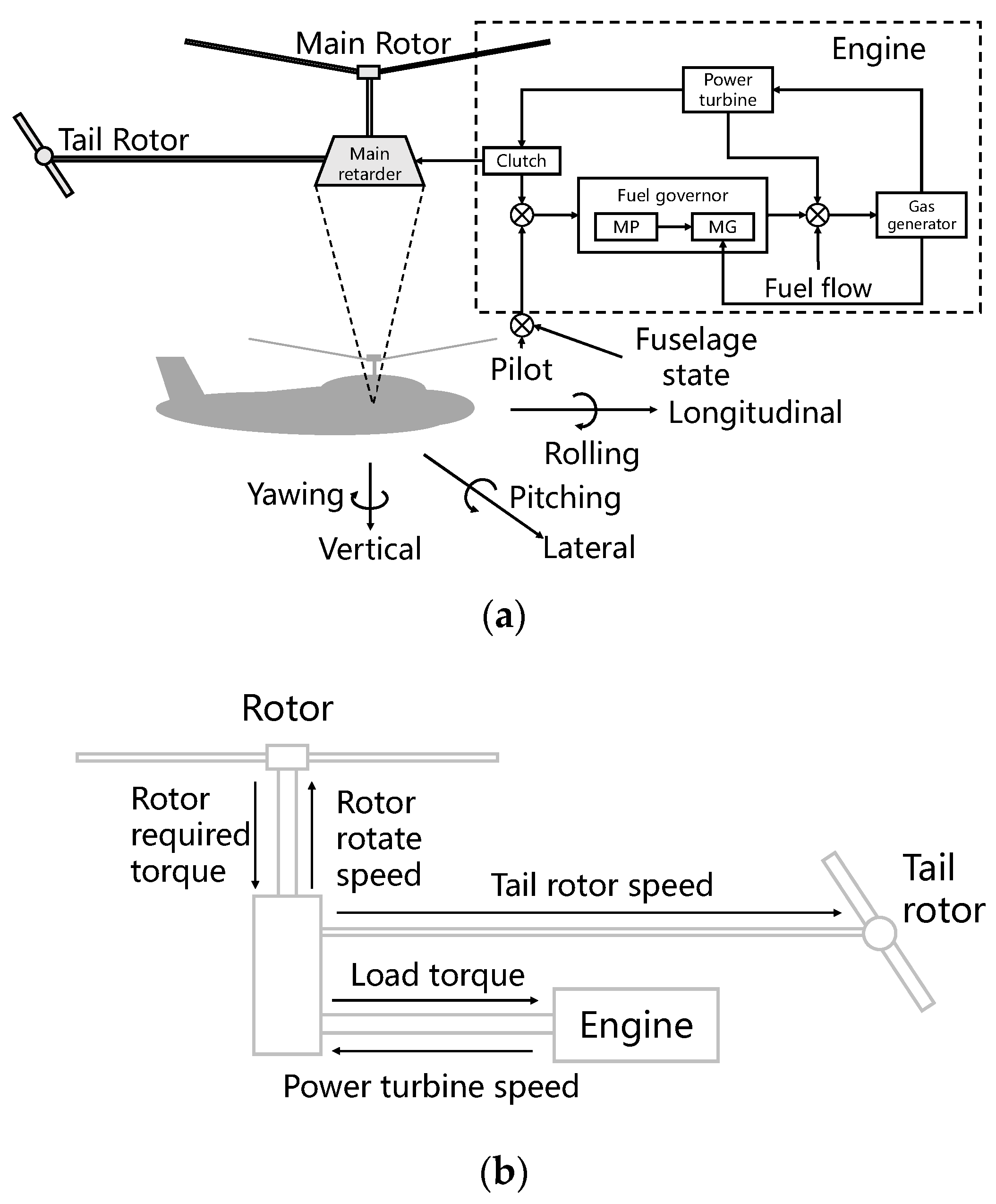
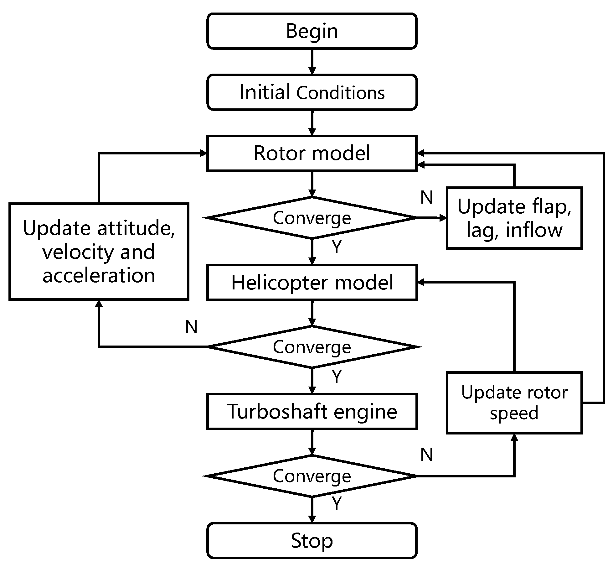
2.3. Helicopter–Engine Coupling Model (HECM)

We establish a helicopter–engine coupling model (HECM) based on the power-matching relationship. As depicted in Figure 2, the helicopter’s main rotor and tail rotor are directly connected to the engine. The helicopter’s torque demand corresponds to the load imposed on the turboshaft engine, thus directly affecting the engine’s output. The engine’s hysteresis effect introduces the phenomenon of the engine output lagging behind the power demand of the helicopter. This power mismatch can change the rotor rotation speed, altering the helicopter’s power requirements.
The central element of the HECM resides in the coupling dynamics between the main rotor and the engine. Because the engine output lag significantly influences the main rotor speed, rotor state change has the most apparent impact on the helicopter’s flight status. Based on the power-matching relationship and torque balance relationship on the main rotor spindle, we can obtain the main rotor engine coupling relationship:
P = Q × Ω Ω ˙ = ( Q E Q r e q ) / J ,
where P means power; Q represents torque; and Ω is the rotation speed. J is the moment of inertia. The HECM calculating flow chart is shown in Figure 3.
The nonlinear flight dynamics model of HECM is established below:
x ˙ = f ( x , u , t )
where x = x B , x F , x L , x I , x e n g is the state vector; u = [ δ c o l , δ l a t , δ l o n , δ p e d , w f ] is the control vector; and t is time. x B is the body motion vector; x F is the rotor flap motion vector; x L is the rotor lead–lag motion vector; x I is the rotor inflow vector; and x e n g is the engine’s internal state quantity.
      x = x B , x F , x L , x I , x e n g     x B = [ u , v , w , p , q , r , ϕ , θ , ψ ]     x F = [ β 1 , β 2 , β 3 , β 4 , β ˙ 1 , β ˙ 2 , β ˙ 3 , β ˙ 4 ]     x L = [ ζ 1 , ζ 2 , ζ 3 , ζ 4 , ζ ˙ 1 , ζ ˙ 2 , ζ ˙ 3 , ζ ˙ 4 ]       x I = [ v i 0 , v i c , v i s ] x e n g = N g , N p ,   P 3 ,   P 41 ,   P 45         u = [ δ c o l , δ l a t , δ l o n , δ p e d , w f ] ,
where u, v, and w denote the helicopter linear velocity; p, q, and r denote the helicopter angular velocity; and ϕ , θ , ψ are the helicopter Euler angle. β is the flap angle; β ˙ is the flap rate; ζ is the lead–lag angle; and ζ ˙ is the lead–lag rate. v i 0 , v i c , v i s are three components of dynamic inflow. N g , N p , P 3 , P 41 , P 45 are the engine gas generator speed, power turbine speed, compressor inlet pressure, gas turbine inlet pressure, and power turbine inlet pressure. δ c o l , δ l a t , δ l o n , δ p e d , w f is the collective pitch stick, lateral cyclic stick, longitudinal cyclic stick, pedal position, and fuel flow.

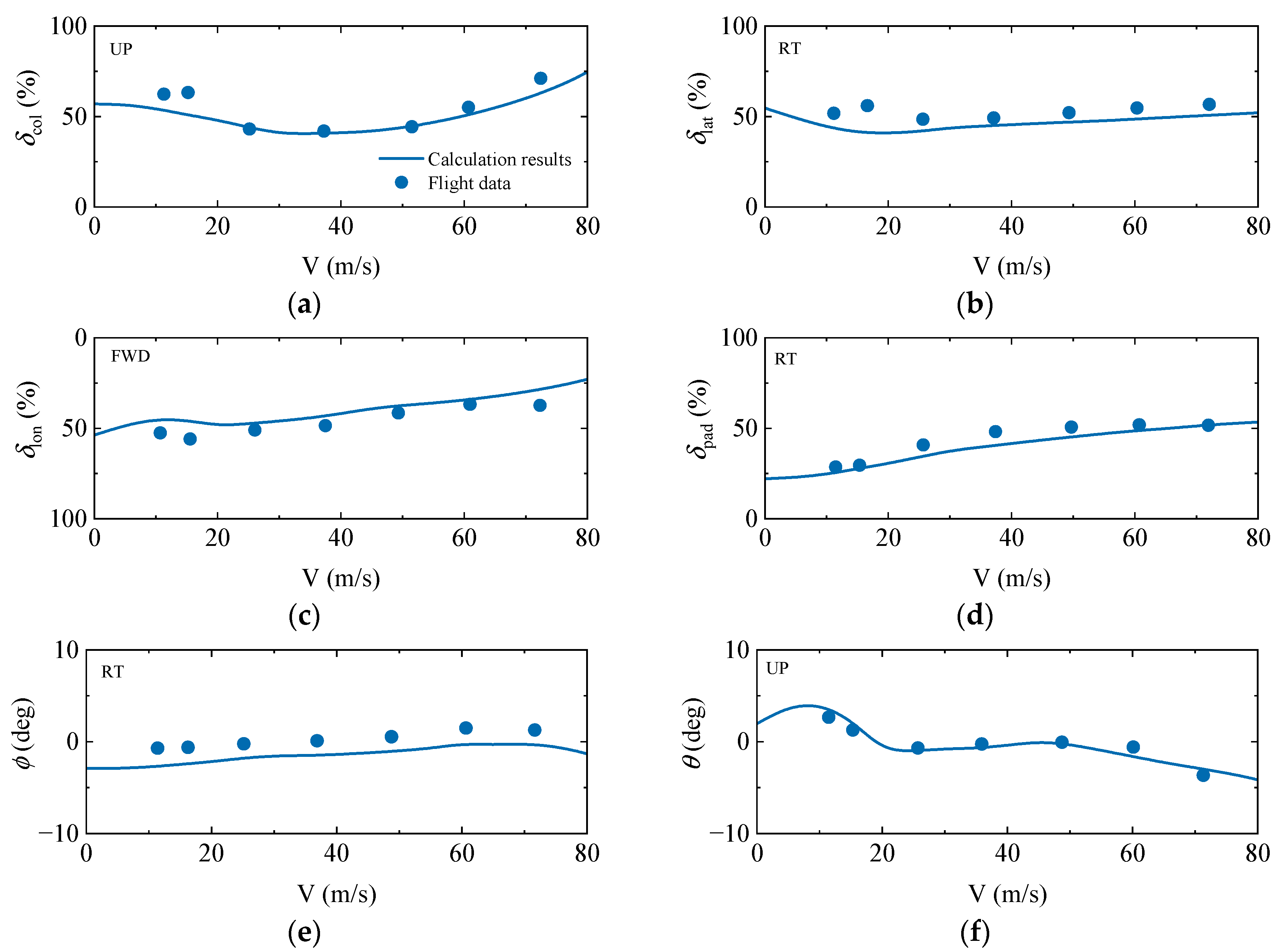
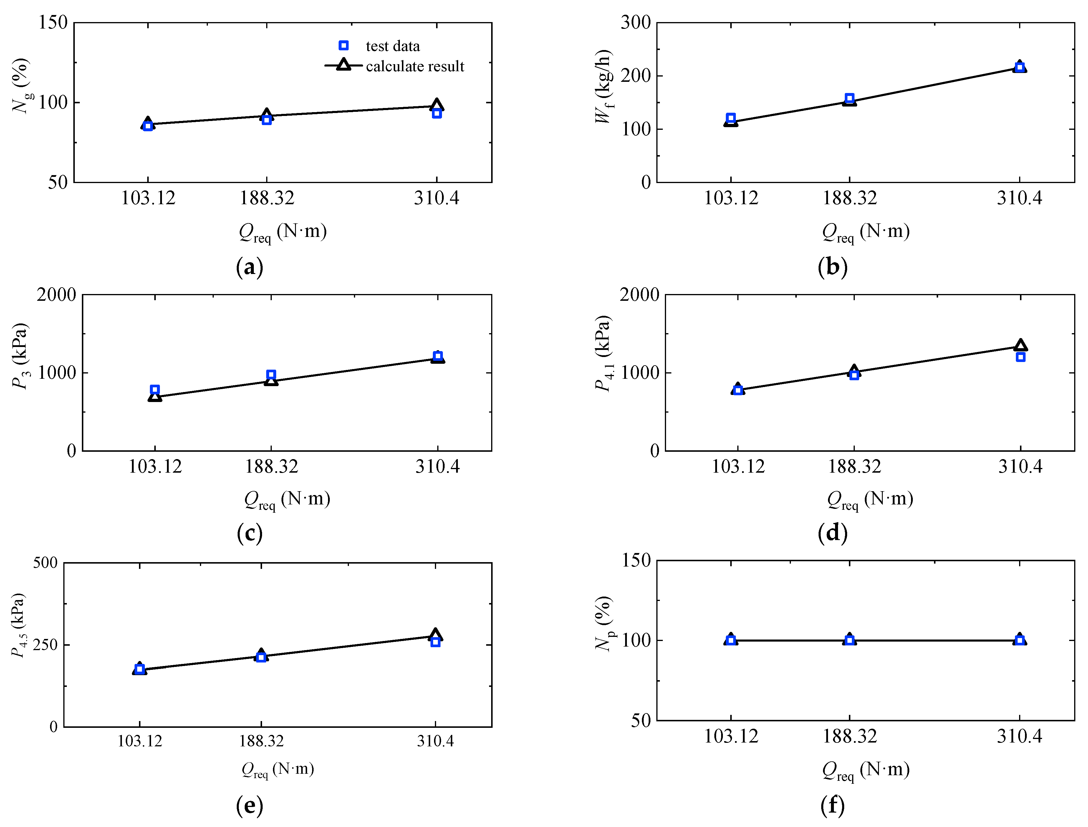
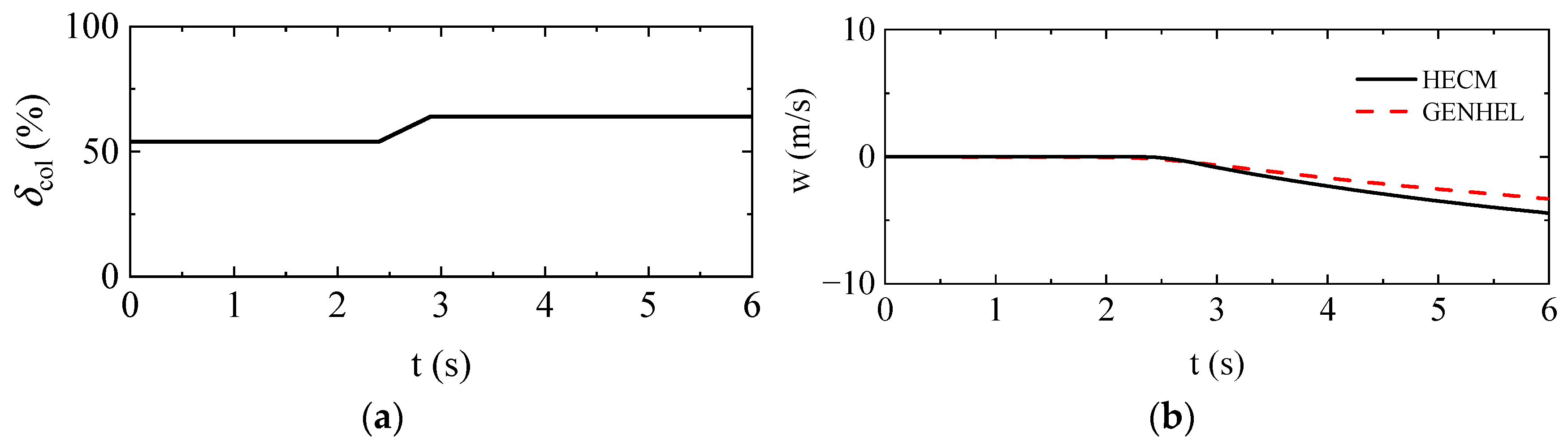
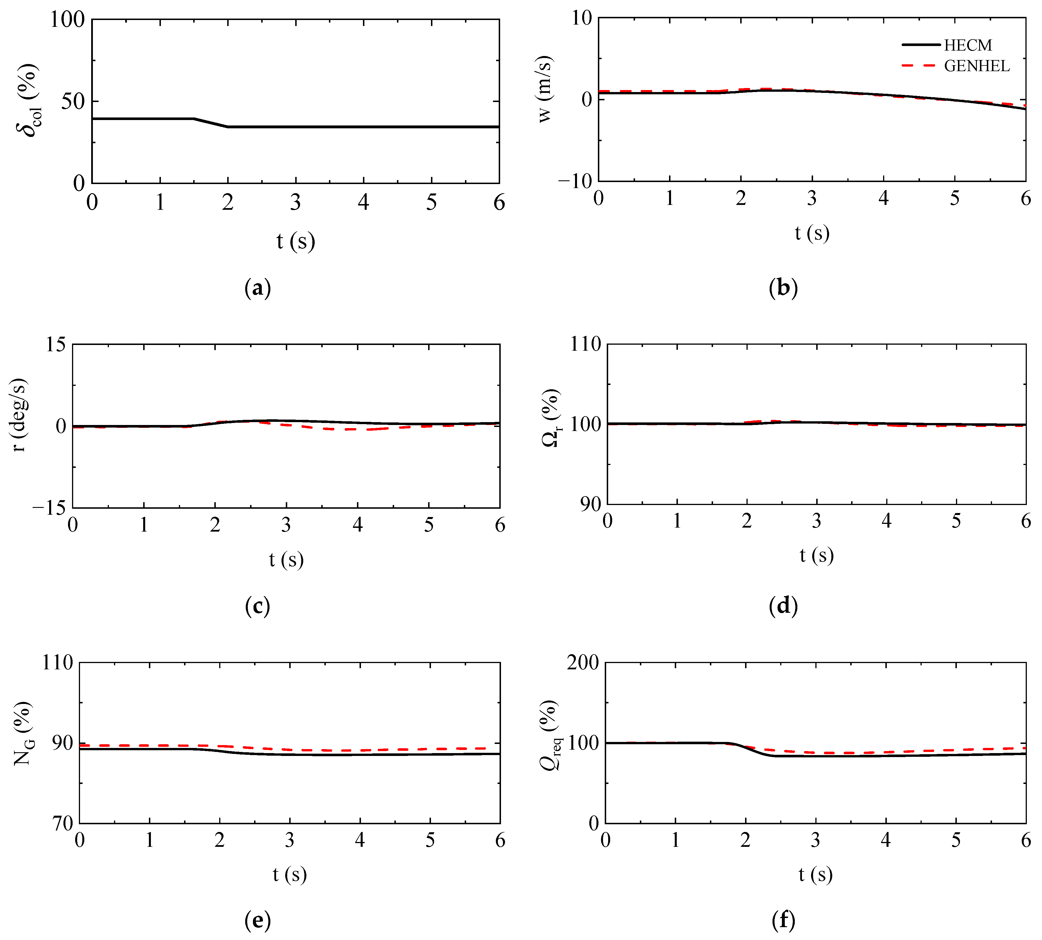
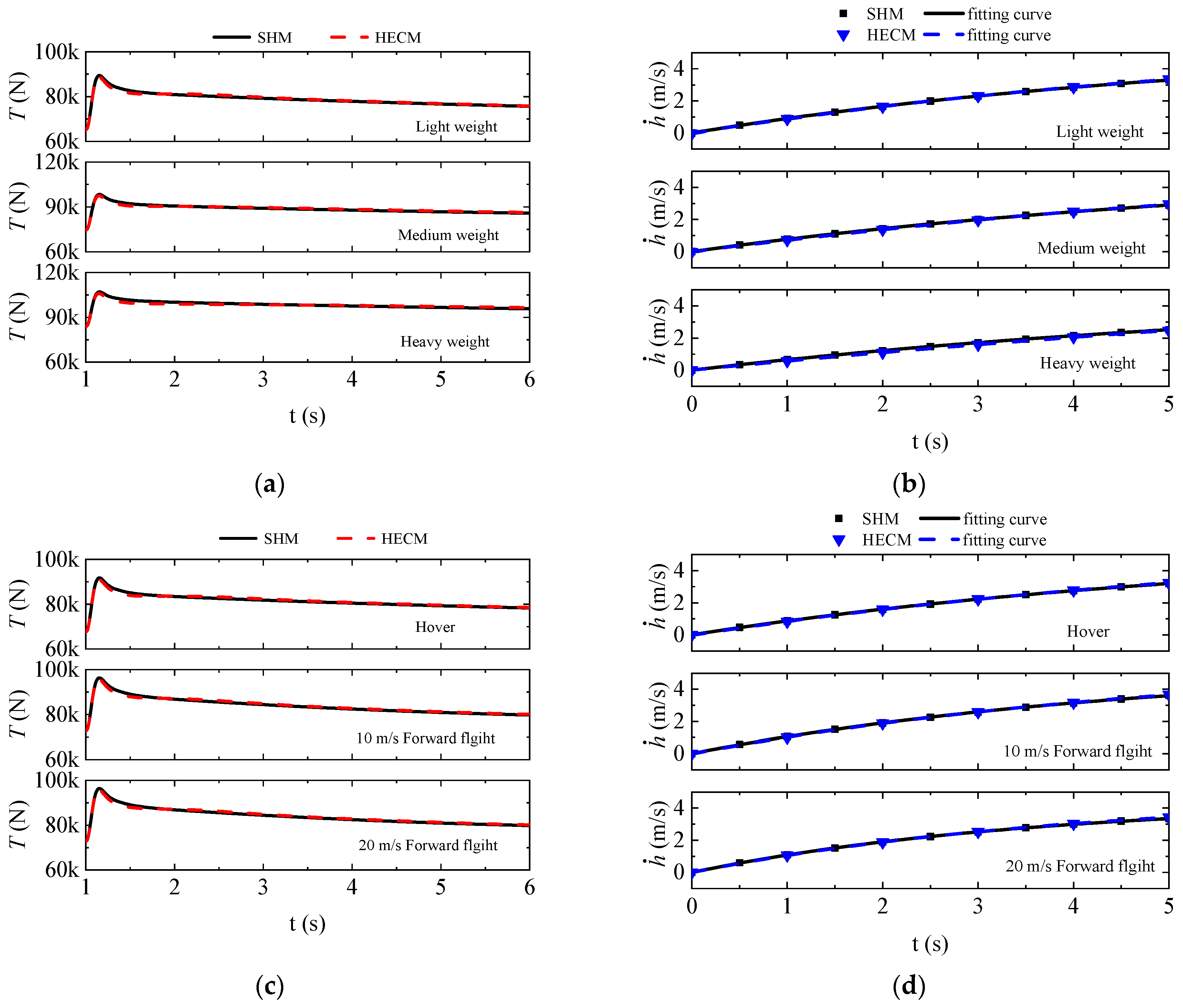
2.4. Model Validation

We validate the helicopter trim results using flight test data from the UH-60A helicopter conducted by the United States Army Aviation Engineering Flight Activity (AEFA) [39,40]. The helicopter’s weight is 7257.5 kg, with its center of gravity (C.G.) positioned at (8.92, 0, 5.88) m, and it operates at a density altitude of 1600.2 m. Figure 4 illustrates the helicopter trim result: collective pitch stick, lateral cyclic stick, longitudinal cyclic stick, pedal position, roll angle and pitch angle, and the flight test data obtained from AEFA. The calculated steady-state variables are in agreement with the flight test data.
We verify the turboshaft engine by test results [38]. The power turbine speed is 2188.1 rad/s, while the gas turbine speed registers at 4681.0 rad/s. Figure 5 compares the engine thermoaerodynamics calculation results; gas generator speed, power turbine speed, fuel flow, compressor inlet pressure, gas turbine inlet pressure, power turbine inlet pressure, and the calculated steady-state variables agree with the flight test data.
Furthermore, the dynamic response of the HECM is validated using the Sikorsky general helicopter (GENHEL) model [39,40], which has good credibility and has been implemented in the famous NASA’s Ames Research Center. The transient step response characteristics of UH-60A in hover and 60 knots forward flight are calculated. As depicted in Figure 6 and Figure 7, a comparison of the dynamic response results of HECM and the GENHEL model reveals similarities in vertical speed, heading speed responses, and the behaviors of main rotor required torque, rotor speed, and gas generator speed. Consequently, we conclude that the HECM model established in this study exhibits reliability and is suitable for subsequent simulations and handling quality assessment.

3. Handling Qualities Assessment

The coupling between the helicopter and the engine can deteriorate the helicopter’s handling quality. First, the engine output lag introduces a lag in engine output power, affecting torque response and collective–yaw coupling characteristics. Additionally, variation in rotor speed can impact the rotor thrust, leading to deterioration in height response characteristics. Consequently, we focus on three key indicators in the ADS-33E-PRF handling quality specifications closely related to the engine dynamic characteristics: torque response, height response, and collective–yaw coupling characteristics. These indicators are used to assess the engine’s influence on helicopter handling quality quantitatively. For each criterion, the requirements are evaluated between Level 1 (good) and Level 3 (bad).
We use the UH-60A helicopter as our sample aircraft to conduct our analysis. The helicopter operates at an altitude of 1649.27 m, with the C.G. is at (9.13, 0, 5.91) m. We have selected 12 test cases, as presented in Table 1, to compare helicopter handling qualities under varying weights and forward speeds using the HECM and single helicopter model (SHM). SHM with the ideal engine that can instantly match the helicopter’s required torque.

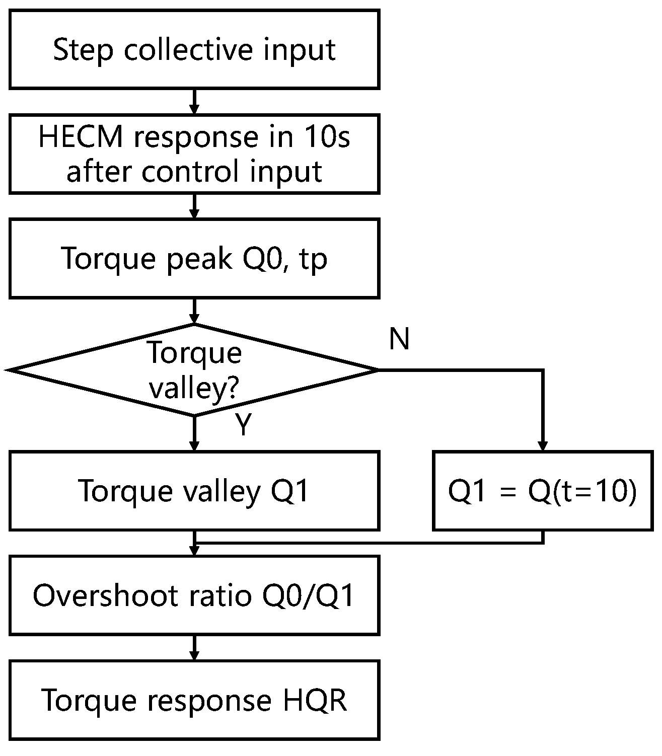
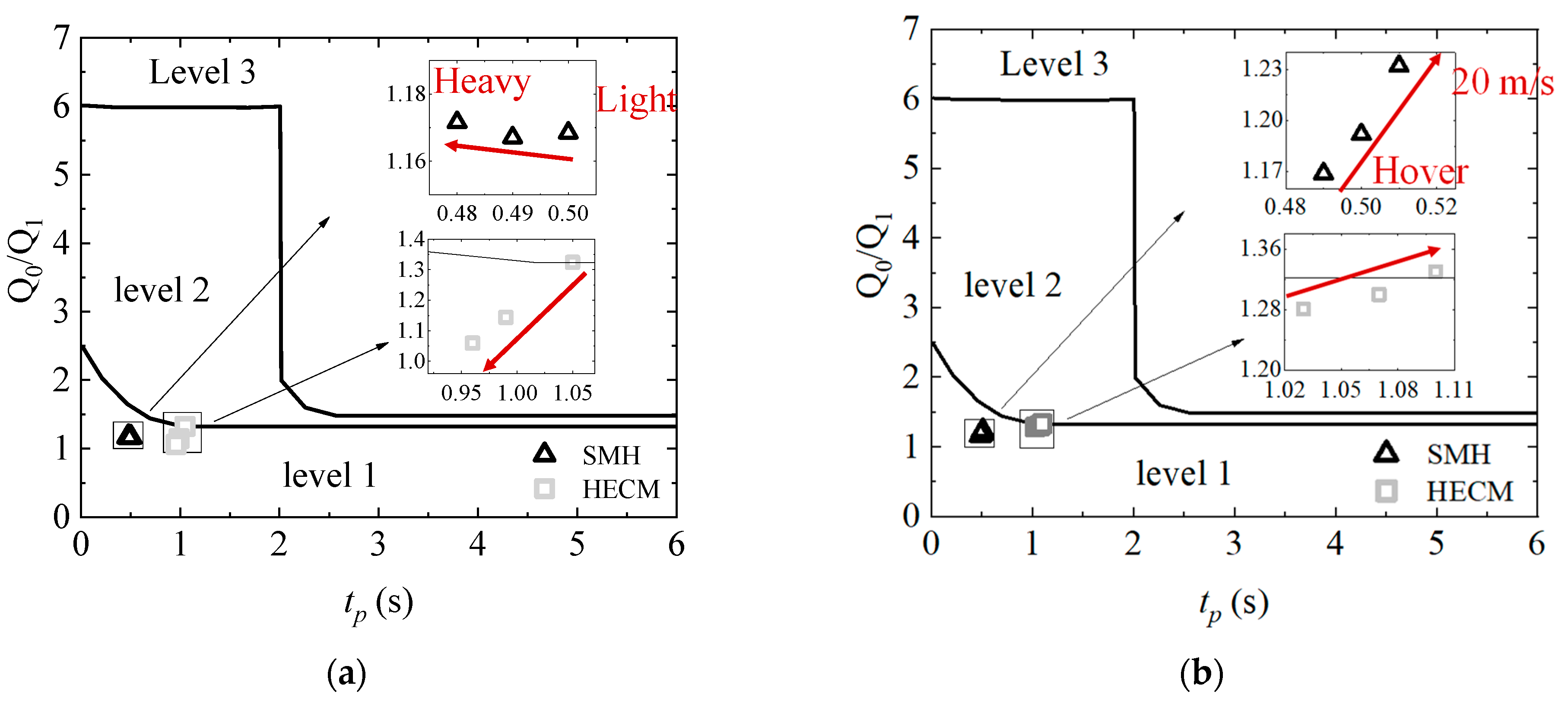
3.1. Torque Response HQR Assessment

The torque dynamic response characteristics were evaluated under hover and low-speed forward flight conditions, following the relevant ADS-33E-PRF regulations. The evaluation procedure is illustrated in Figure 8, recording the rotor torque response time history after a step collective input. The handling quality of the torque response is assessed using the overshoot ratio (OR) versus the time-to-the-first peak t p . When the first local minimum of torque does not occur within the 10 s window, the response valley ( Q 1 ) equals the value observed at the end of the 10 s. The torque response results are obtained under the influence of the step collective input.
The rotor speed and torque response curves are shown in Figure 9. The distribution of torque dynamic characteristics for the aircraft is depicted in Figure 10. The engine output lag degrades the helicopter’s torque response HQR. With the increasing helicopter weight, the engine’s output lag reduces the torque response handling quality to Level 2. The impact of the engine on the torque overshoot ratio decreases from 0.155 to −0.113. Additionally, the effect on the torque response peak time reduces from 0.55 s to 0.48 s. Because as the helicopter weight increases, rotor torque also increases, consequently, heavier helicopters exhibit slower rotor speed recovery under the same collective stick control, resulting in a smaller torque overshoot ratio and reduced engine impact on torque response.
As forward flight speed increases, the engine output lag decreases torque response handling quality to Level 2. The engine’s impact on the torque overshoot ratio Q 0 / Q 1 decreases from 0.112 to 0.098. Meanwhile, the effect on torque response peak time t p increases from 0.54 s to 0.59 s. This effect is because as the helicopter’s required torque increases, the rate of change in rotor speed slows down, leading to a decrease in the rotor torque overshoot ratio caused by engine output. Consequently, the adverse impact of engine dynamic characteristics on helicopter torque response handling quality diminishes.

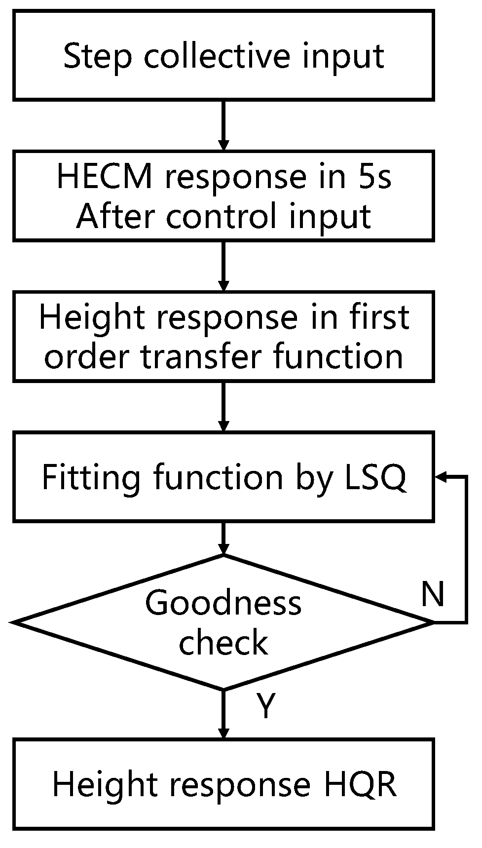
3.2. Height Response HQR Assessment

The procedure for calculating the altitude response handling quality, as outlined in the ADS-33E-PRF criteria, is detailed in Figure 11. It specifies that pitch, roll, and heading excursions remain essentially constant during this evaluation. Moreover, the vertical velocity response must exhibit a qualitative first-order shape for at least 5 s following a step collective input. The equivalent first-order transfer function of vertical rate to the collective stick input is defined as follows:
h ˙ δ col = K exp ( τ h ˙ e q s ) T h ˙ e q s + 1 ,
in which h ˙ is the vehicle’s vertical speed. K, τ h ˙ e q , T h ˙ e q denote the coefficient of the first-order transfer function.
Equivalent system parameters are determined through the time-domain fitting method, with a response time interval not exceeding t = 0.05 s within a 5 s timeframe. A three-variable nonlinear least squares algorithm is employed to obtain the fitted curve.
The definition of the sum of squares of the error e 2 and the coefficient of determination r 2 , which represents the goodness of fit of the estimated curve, is defined as follows:
e 2 = i = 1 n ( h ˙ ( t = t i ) h ˙ e s t ( t = t i ) ) 2 ,
r 2 = Σ i = 1 n ( h ˙ e s t ( t = t i ) h ˙ m ) 2 Σ i = 1 n ( h ˙ ( t = t i ) h ˙ m ) 2 ,
in which h ˙ e s t is the estimated vertical speed; and h ˙ m is the mean of observed vertical speed.
As ruled in the criterion, the coefficient of determination r 2 is expected to fall within the range of [0.97, 1.03]. The fitting curve parameters are listed in Table 2. The vertical velocity response maintains a first-order shape in hover and low-speed forward flight conditions. The coefficient of determination of all cases falls within the specified range, indicating that the calculation results meet the requirements of the criterion, and the smallest r 2 (=0.99980) is occurred at SHM, 20 m/s forward flight condition. The biggest T h ˙ e q is 14.4415, which occurs in at HECM, heavy weight condition. Figure 12 shows the response curve of rotor thrust and vertical speed and the velocity least squares method fitting curve.
Based on LSQ calculation results in Table 2, we can figure out the altitude HQR for all conditions. As depicted in Figure 13, the lag in engine output significantly reduces the handling quality Level of the helicopter’s altitude response characteristics. With an increase in helicopter weight, the influence of the engine results in the helicopter’s altitude response HQR transitioning from Level 1 to Level 2. The engine’s output lag leads to a decrease in the helicopter’s altitude response fitting function coefficient τ h ˙ e q from 0.028 to −0.013, and to T h ˙ e q increasing from 0.463 s to 7.24 s. Conversely, as the helicopter’s forward flight speed increases, the impact caused by the engine decreases from Level 2 to Level 1. The engine impact reduces the helicopter response fitting function coefficient τ h ˙ e q from 0.030 to 0.005, and T h ˙ e q from 6.75 to 4.03 s. Therefore, it can be concluded that the adverse effect of engine dynamic response on the handling quality of helicopter altitude characteristics intensifies with the increase in flight weight and decreases with the rise of forward flight speed.
From an energy perspective, when the rotor speed changes, the kinetic energy stored in the rotor is converted into the helicopter’s translational kinetic energy, compensating for the impact of insufficient engine power. As flight weight increases, rotor thrust also increases, and the duration of speed fluctuations resulting from engine output power becomes longer and exacerbates the adverse effects on rotor thrust, reducing the helicopter’s altitude response handling quality. From an energy standpoint, as flight weight increases, the kinetic energy stored in rotor rotation becomes relatively insufficient, resulting in a more pronounced reduction in rotor speed under the same control input. Consequently, the helicopter’s altitude response handling quality rating experiences a significant decline with increasing flight weight.
On the other hand, with an increase in forward flight speed, the engine’s output torque decreases, resulting in reduced rotor speed fluctuations and ultimately improving the helicopter’s altitude response control quality. The impact of engine dynamic characteristics on the helicopter’s altitude HQR at different forward speeds is negligible. Therefore, when the forward flight speed changes, the altitude response handling quality influenced by engine dynamic characteristics does not significantly decrease.

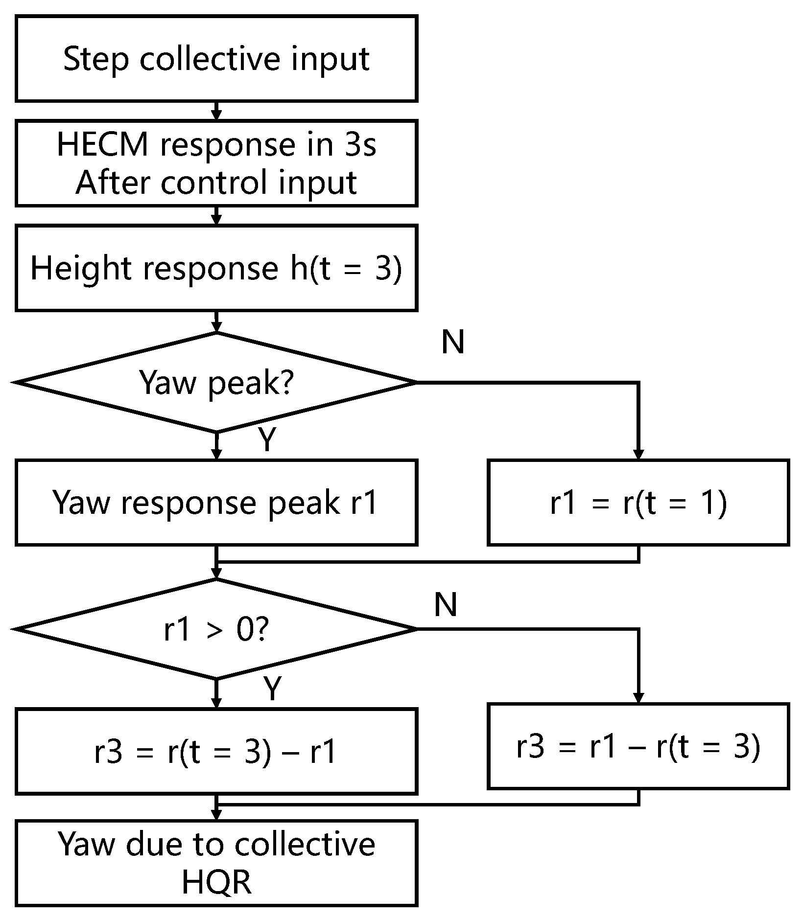
3.3. Yaw Due to Collective Input HQR Assessment

The handling quality specification explicitly addresses inter-axis coupling in rotorcraft, which means that maneuvering inputs applied to achieve a response in one axis must not result in an inappropriate response in one or more of the other axes. The engine dynamic characteristics mainly affect the helicopter’s collective–yaw inter-axis coupling. Figure 14 illustrates the sequence of calculating collective–yaw coupling HQR. After the step collective signal input, there should be no objectionable yaw oscillations, and oscillations with yaw rates greater than 5 degrees/second are considered undesirable. The direction hold can be relaxed if the rotorcraft is equipped with a direction hold controller.
After control input, the yaw rate and vertical velocity response are calculated within 3 s timeframes starting from initiating the step collective input. The highest yaw rate within 3 s is denoted as r 1 . In cases where no peak occurs within the initial 3 s, the yaw rate at the end of the first second, denoted as r(1), is utilized. If multiple peaks occur, the maximum value of the wave peak is considered. The yaw rate response value at the end of the 3 s is referred as r 3 :
r 3 = r ( 3 ) r 1   for   r 1 > 0 r 3 = r 1 r ( 3 )   for   r 1 < 0
The response results in Figure 15 depict a pronounced reverse process in the dynamic response of the yaw rate after the introduction of the engine model. This phenomenon can be attributed to the torque mismatch between the rotor and tail rotor on the yaw axis of the helicopter. When the collective signal is input, the engine output lag causes the torque imbalance on the rotor axis, leading to the helicopter’s reverse yaw motion.
The handling quality of the helicopter’s collective–yaw coupling characteristics under different weights and forward speeds is shown in Figure 16. The engine’s dynamic characteristics contribute to the helicopter’s collective–yaw coupling HQR deterioration. The collective–yaw coupling HQR decreases to Level 2 as the flight weight increases. The impact of engine output lag on r 3 / | h ˙ 3 | increases from −0.148 to −0.785. Conversely, the impact on | r 1 / h ˙ 3 | decreases from 0.007 to −0.216. The lag in engine output torque alters the direction of the yaw rate | r 1 / h ˙ 3 | , leading to a change in the sign of yaw rate changes, further exacerbating the adverse impact on the collective–yaw coupling characteristics.
On the other hand, as the forward speed increases, the engine’s impact on the collective yaw coupling characteristics does not diminish. In contrast to the altitude response, the adverse influence of the engine on the yaw response is further exacerbated. After increasing the forward speed, the impact of the engine on r 3 / | h ˙ 3 | increased from −0.269 to −0.352, reflecting a 41.8% increase, and the effect on | r 1 / h ˙ 3 | increased from −0.021 to 0.097, indicating an 18.2% increase. As the helicopter’s forward speed increases, the adverse effect of engine output torque lag on the yaw direction is further exacerbated, resulting in a decline in the collective–yaw coupling HQR.

4. Conclusions

We constructed the helicopter–engine coupling model (HECM) based on the power-matching relationship between the rotor and engine and verified the model via AEFA test results. We assess the influence of engine dynamic characteristics on helicopter handling quality by comparing HECM and the single helicopter model (SHM) and calculating the results. Based on previous research, the following conclusions can be drawn:
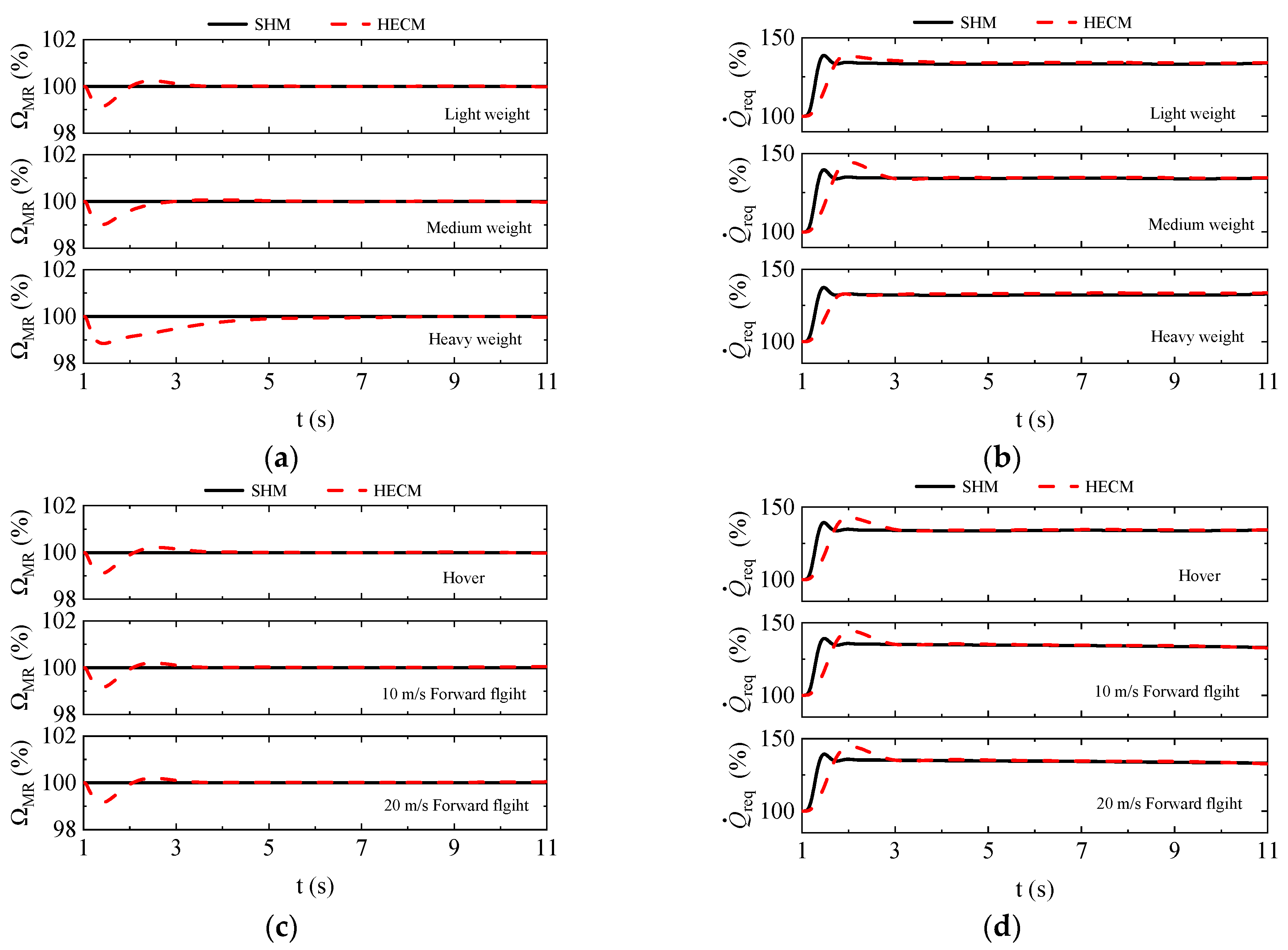
  • Engine output lag diminishes the handling quality of the helicopter’s torque response as the helicopter flight weight increases. When the required torque for the aircraft rises, the impact of engine dynamic characteristics on the helicopter’s torque response HQR is significantly reduced.
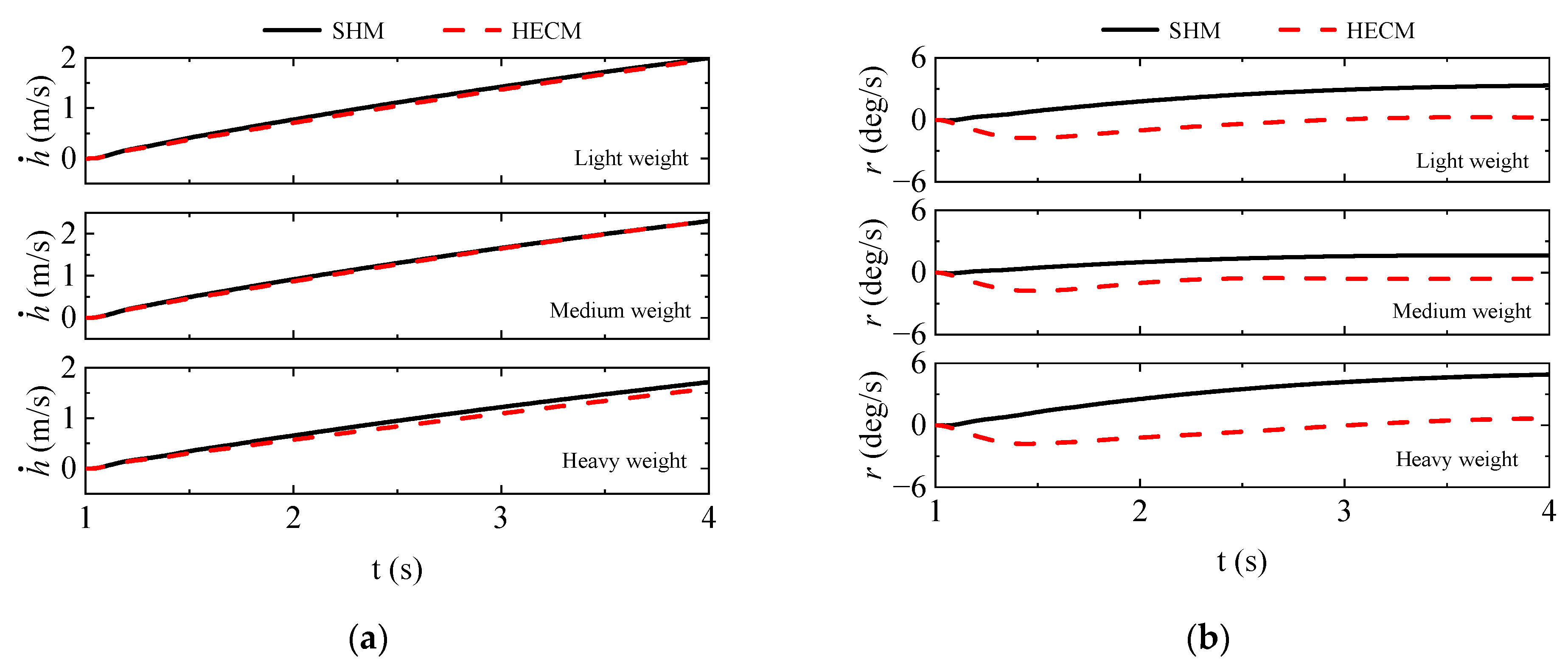
  • Engine dynamic characteristics deteriorate the helicopter’s height response HQR. The helicopter flight weight substantially impacts the influence of engine output lag on altitude response. At higher flight weight, the slower recovery of engine output results in the conversion of the rotor rotation kinetic energy into translational kinetic energy, significantly affecting rotor thrust and leading to a decline in the helicopter’s altitude response HQR.
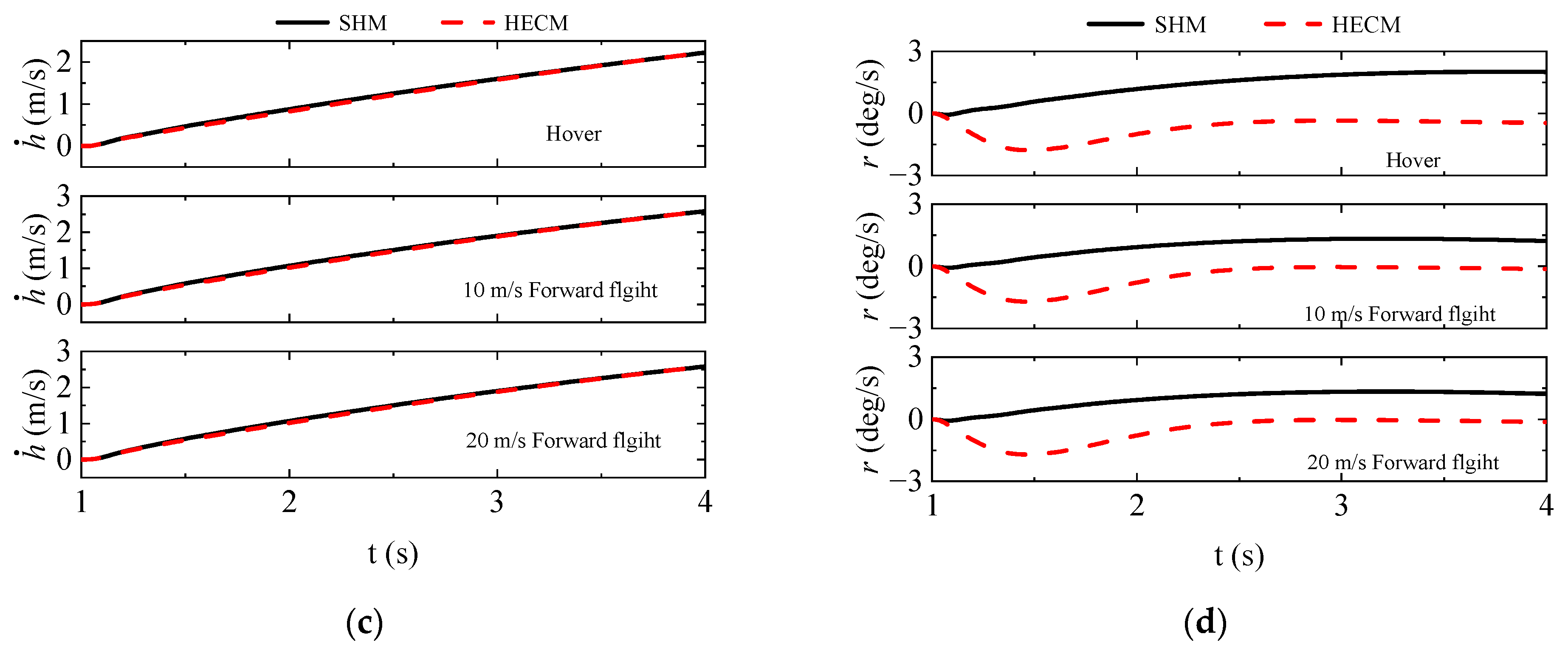
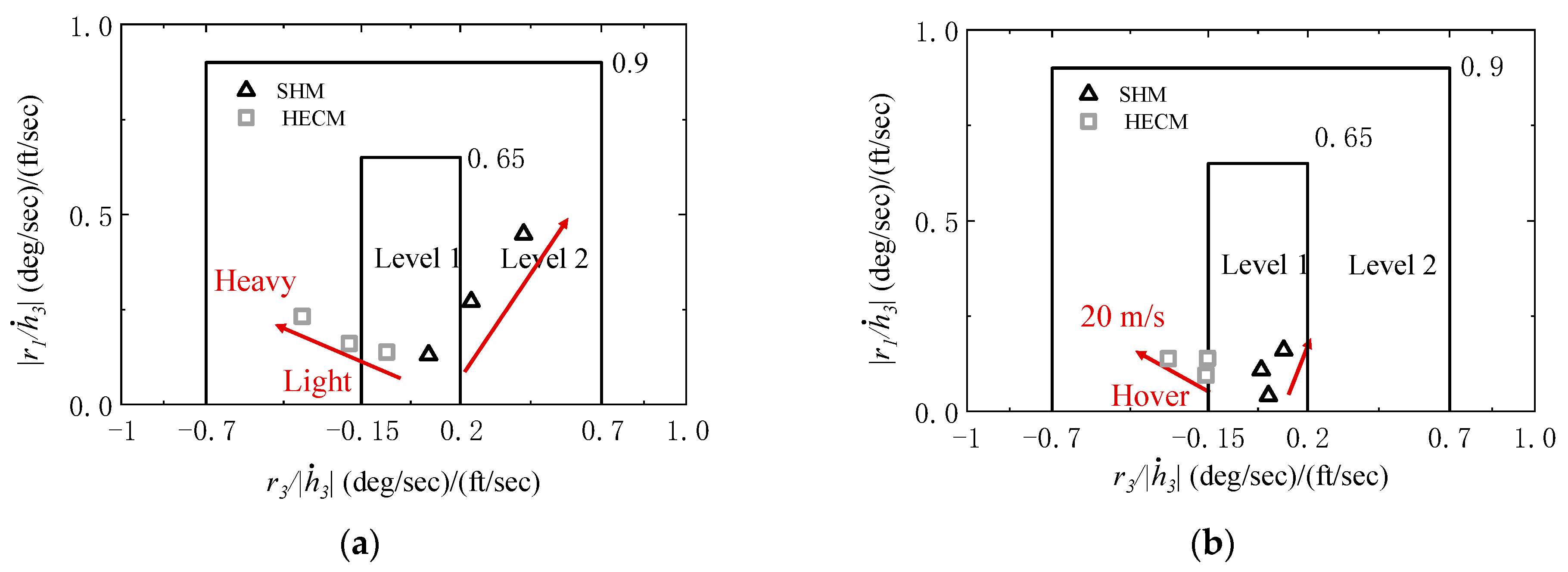
  • The dynamic coupling effect of the rotor/engine system reduces the helicopter’s collective–yaw coupling HQR. As forward flight speed increased to 20 m/s, the reverse change in yaw rate induced by engine output lag became most pronounced. The r 3 / | h ˙ 3 | increased by 41.8%, further decreasing the collective–yaw coupling HQR. This analysis provides valuable insight into the impact of engine dynamic characteristics on helicopter handling quality and offers guidance for designing helicopter/engine coupling control laws.

Author Contributions

Conceptualization, Y.W., Y.Y. and R.C.; methodology, Y.W., L.W. and R.C.; software, Y.W. and L.W.; validation, Y.W.; formal analysis, Y.W.; investigation, Y.W.; resources, Y.W.; data curation, Y.W.; writing—original draft preparation, Y.W.; writing—review and editing, R.C., Y.Y. and L.W.; visualization, Y.W.; supervision, R.C. and Y.Y.; project administration, R.C.; funding acquisition, R.C. All authors have read and agreed to the published version of the manuscript.

Funding

This research received no external funding.

Informed Consent Statement

Not applicable.

Data Availability Statement

The data presented in this study are available on request from the corresponding author. The data are not publicly available due to privacy or ethical restrictions.

Conflicts of Interest

The authors declare no conflicts of interest.

References

  1. Chen, R.; Yuan, Y.; Thomson, D. A Review of Mathematical Modelling Techniques for Advanced Rotorcraft Configurations. Prog. Aerosp. Sci. 2021, 120, 100681. [Google Scholar] [CrossRef]
  2. Baskett, B.J.; Larry, O.D. Aeronautical Design Standard Performance Specification Handling Qualities Requirements for Military Rotorcraft; United States Army Aviation and Missile Command: Redstone Arsenal, AL, USA, 2000. [Google Scholar]
  3. Celi, R. Calculation of ADS-33 quickness parameters with application to design optimization. In Proceedings of the 29th European Rotorcraft Forum, Friedrichshafen, Germany, 16–18 September 2003. [Google Scholar]
  4. Luria, F.; Smith, F.S. ADS-33 Handling Qualities Evaluation of the UH-60M Fly-By-Wire Demonstration Aircraft. In Proceedings of the American Helicopter Society 68th Annual Forum, Fort Worth, TX, USA, 1–3 May 2012. [Google Scholar]
  5. Malpica, C.; Theodore, C.R.; Lawrence, B.; Blanken, C.L. Handling Qualities of Large Rotorcraft in Hover and Low Speed; NASA/TP-2015-216656; Ames Research Center: Moffett Field, CA, USA, 2015.
  6. Lawrence, B.; Theodore, C.R.; Johnson, W.; Berger, T. A handling qualities analysis tool for rotorcraft conceptual designs. Aeronaut. J. 2018, 122, 960–987. [Google Scholar] [CrossRef]
  7. Gerosa, G.; Zanoni, A.; Panza, S.; Masarati, P.; Lovera, M. A handling qualities oriented approach to rotorcraft conceptual design. In Proceedings of the AHS International 74th Annual Forum & Technology Display, Phoenix, AZ, USA, 14–17 May 2018. [Google Scholar]
  8. Tischler, M.; Colbourne, J.; Morel, M.; Biezad, D.; Levine, W.; Moldoveanu, V.; Tischler, M.; Colbourne, J.; Morel, M.; Biezad, D.; et al. CONDUIT—A new multidisciplinary integration environment for flight control development. In Proceedings of the Guidance, Navigation, and Control Conference, New Orleans, LA, USA, 11–13 August 1997. [Google Scholar]
  9. Horn, J.F.; Guo, W.; Ozdemir, G.T. Use of rotor state feedback to improve closed-loop stability and handling qualities. J. Am. Helicopter Soc. 2012, 57, 1–10. [Google Scholar] [CrossRef]
  10. Horn, J.F. Non-Linear Dynamic Inversion Control Design for Rotorcraft. Aerospace 2019, 6, 38. [Google Scholar] [CrossRef]
  11. Türe, U.; Sarsilmaz, S.B.; Sahin, I.H. Optimization of Flight Control System and Handling Quality Evaluation of a Limited Authority Helicopter. In Proceedings of the AHS International’s 71st Annual Forum and Technology Display, Virginia Beach, VA, USA, 5–7 May 2015. [Google Scholar]
  12. Ji, H.; Chen, R.; Li, P. Analysis of helicopter handling quality in turbulence with recursive Von karman model. J. Aircr. 2017, 54, 1631–1639. [Google Scholar] [CrossRef]
  13. Yuan, Y.; Thomson, D.; Anderson, D. Aerodynamic Uncertainty Quantification for Tiltrotor Aircraft. Aerospace 2022, 9, 271. [Google Scholar] [CrossRef]
  14. Yuan, Y.; Thomson, D.; Anderson, D. Faster-than-realtime inverse simulation method for tiltrotor handling qualities investigation. Aerosp. Sci. Technol. 2022, 124, 107516. [Google Scholar] [CrossRef]
  15. Yan, X.; Yuan, Y.; Chen, R. Research on Pilot Control Strategy and Workload for Tilt-Rotor Aircraft Conversion Procedure. Aerospace 2023, 10, 742. [Google Scholar] [CrossRef]
  16. Yan, X.; Chen, R. Augmented flight dynamics model for pilot workload evaluation in tilt-rotor aircraft optimal landing procedure after one engine failure. Chin. J. Aeronaut. 2019, 32, 92–103. [Google Scholar] [CrossRef]
  17. Talbot, P.D.; Tinling, B.E.; Decker, W.A.; Chen, R.T.N. A Mathematical Model of a Single Main Rotor Helicopter for Piloted Simulation; Ames Research Center: Moffett Field, CA, USA, 1982.
  18. Chen, R.T.N. Effects of Primary Rotor Parameters on Flapping Dynamics; Ames Research Center: Moffett Field, CA, USA, 1980.
  19. Corliss, L.D. The Effects of Engine and Height-Control Characteristics on Helicopter Handling Qualities. J. Am. Helicopter Soc. 1983, 28, 56–62. [Google Scholar]
  20. Cho, H.; Ryu, H.; Shin, S.J.; Cho, I.-J.; Jang, J.-S. Development of a Coupled Analysis Regarding the Rotor/Dynamic Components of a Rotorcraft. J. Mech. Sci. Technol. 2014, 28, 4841–4856. [Google Scholar] [CrossRef]
  21. Liu, K.; Mittal, M.; Prasad, J.; Scholz, C. A Study of Coupled Engine/Rotor Dynamic Behavior. In Proceedings of the 51st Annual Forum of the American Helicopter Society, Fort Worth, TX, USA, 9–11 May 1995. [Google Scholar]
  22. Zhang, H.; Wang, J.; Chen, G.; Yan, C. A New Hybrid Control Scheme for an Integrated Helicopter and Engine System. Chin. J. Aeronaut. 2012, 25, 533–545. [Google Scholar] [CrossRef]
  23. Wang, Y.; Song, J.; Zhong, W.; Zhang, H. Rotational Speed Optimization of Coaxial Compound Helicopter and Turboshaft Engine System. J. Aerosp. Eng. 2023, 36, 04023042. [Google Scholar] [CrossRef]
  24. Guglieri, G. Effect of Drive Train and Fuel Control Design on Helicopter Handling Qualities. J. Am. Helicopter Soc. 2000, 46, 14–22. [Google Scholar] [CrossRef]
  25. Richardson, D.A.; Alwang, J.R. Engine/Airframe/Drive Train Dynamic Interface Documentation; Final Report; Boeing Vertol, Co.: Philadelphia, PA, USA, 1978. [Google Scholar]
  26. Hanson, H.; Balke, R.; Edwards, B.; Riley, W.; Downs, B. Engine/Airframe/Drive Train Dynamic Interface Documentation; Bell Helicopter Textron: Fort Worth, TX, USA, 1978. [Google Scholar]
  27. Hull, R. Development of a Rotorcraft/Propulsion Dynamics Interface Analysis: Volume I; Ames Research Center: Moffett Field, CA, USA, 1982.
  28. Mihaloew, J.R.; Ballin, M.G.; Ruttledge, G. Rotorcraft Flight-Propulsion Control Integration: An Eclectic Design Concept; Lewis Research Center: Cleveland, OH, USA, 1988. [Google Scholar]
  29. Han, D.; Pastrikakis, V.; Barakos, G.N. Helicopter Performance Improvement by Variable Rotor Speed and Variable Blade Twist. Aerosp. Sci. Technol. 2016, 54, 164–173. [Google Scholar] [CrossRef]
  30. Iwata, T. Integrated Flight/Propulsion Control with Variable Rotor Speed Command for Rotorcraft. Ph.D. Thesis, Stanford University, Stanford, CA, USA, 1996. [Google Scholar]
  31. Guo, W. Flight Control Design for Rotorcraft with Variable Rotor Speed. Ph.D. Thesis, The Pennsylvania State University, State College, PA, USA, 2009. [Google Scholar]
  32. Misté, G.A.; Benini, E. Variable-speed rotor helicopters: Performance comparison between continuously variable and fixed-ratio transmissions. J. Aircr. 2016, 53, 1189–1200. [Google Scholar] [CrossRef]
  33. Wang, Y.; Zheng, Q.; Xu, Z.; Zhang, H. A Novel Control Method for Turboshaft Engine with Variable Rotor Speed Based on the Ngdot Estimator through LQG/LTR and Rotor Predicted Torque Feedforward. Chin. J. Aeronaut. 2020, 33, 1867–1876. [Google Scholar] [CrossRef]
  34. Howlett, J.J. UH-60A Black Hawk Engineering Simulation Program Volume I: Mathematical Model; Ames Research Center: Moffett Field, CA, USA, 1981.
  35. Li, P.; Chen, R. A Mathematical Model for Helicopter Comprehensive Analysis. Chin. J. Aeronaut. 2010, 23, 320–326. [Google Scholar]
  36. Wang, L.; Chen, R. Nonlinear Helicopter Rigid-Elastic Coupled Modeling with Its Applications on Aeroservoelasticity Analysis. AIAA J. 2022, 60, 102–112. [Google Scholar] [CrossRef]
  37. Kim, F.D. Formulation and Validation of High-Order Mathematical Models of Helicopter Flight Dynamics. Ph.D. Thesis, University of Maryland, College Park, MD, USA, 1991. [Google Scholar]
  38. Ballin, M.G. A High Fidelity Real-Time Simulation of a Small Turboshaft Engine; Ames Research Center: Moffett Field, CA, USA, 1988.
  39. Ballin, M.G. Validation of a Real-Time Engineering Simulation of the UH-60A Helicopter; Ames Research Center: Moffett Field, CA, USA, 1987.
  40. Ruttledge, D.G.C. A Rotorcraft Flight/Propulsion Control Integration Study; Sikorsky Aircraft: Stratford, CT, USA, 1986. [Google Scholar]
Figure 1. Schematic of this article.
Aerospace 11 00034 g001
Figure 2. Schematic illustration of the helicopter–engine coupling relationship: (a) coupling between the helicopter and engine [17]; (b) torque/rotate speed coupling between the rotor, tail rotor, and engine.
Aerospace 11 00034 g002
Figure 3. Flowchart outlining the calculation process of HECM.
Aerospace 11 00034 g003
Figure 4. Trimmed characteristics of helicopter: (a) collective pitch stick; (b) lateral cyclic stick; (c) longitudinal cyclic stick; (d) pedal position; (e) roll angle; (f) pitch angle.
Aerospace 11 00034 g004
Figure 5. Trimmed characteristics of turboshaft engine: (a) gas generator speed; (b) power turbine speed; (c) fuel flow; (d) compressor inlet pressure; (e) gas turbine inlet pressure; (f) power turbine inlet pressure.
Aerospace 11 00034 g005
Figure 6. Transient step response characteristics of the helicopter in hover: (a) control signal; (b) vertical speed; (c) yaw rate; (d) main rotor speed; (e) engine gas generator speed; (f) helicopter required torque.
Aerospace 11 00034 g006aAerospace 11 00034 g006b
Figure 7. Transient step response characteristics of the helicopter in forward flight (60 knots): (a) control signal; (b) vertical speed; (c) yaw rate; (d) main rotor speed; (e) engine gas generator speed; (f) helicopter required torque.
Aerospace 11 00034 g007
Figure 8. Torque response HQR assessment procedure.
Aerospace 11 00034 g008
Figure 9. Main rotor speed and torque response curve of the helicopter: (a) main rotor speed, different weight; (b) torque, different weight; (c) main rotor speed, different speed; (d) torque, different speed.
Aerospace 11 00034 g009
Figure 10. Requirement for helicopter torque response dynamic characteristics: (a) helicopter at different weights in hover; (b) helicopter at different forward speeds.
Aerospace 11 00034 g010
Figure 11. Height response HQR assessment procedure (LSQ, least square algorithm).
Aerospace 11 00034 g011
Figure 12. Height response curve of the helicopter in different conditions: (a) rotor thrust, different weights; (b) helicopter vertical velocity fitting curve, different weights; (c) rotor thrust, different speeds; (d) helicopter vertical velocity fitting curve, different speeds.
Aerospace 11 00034 g012
Figure 13. Requirement for helicopter altitude (height) response dynamic characteristics: (a) helicopter height response characteristics in different weights; (b) helicopter height response characteristics in different forward speeds.
Aerospace 11 00034 g013
Figure 14. Yaw response due to collective input HQR assessment procedure.
Aerospace 11 00034 g014
Figure 15. Yaw-due-to-collective coupling response curve: (a) helicopter vertical velocity, different weight; (b) helicopter yaw speed, different weight; (c) helicopter vertical velocity, different speed; (d) helicopter yaw speed, different speed.
Aerospace 11 00034 g015aAerospace 11 00034 g015b
Figure 16. Requirement for helicopter yaw-due-to-collective coupling response dynamic characteristics: (a) different weights; (b) different forward speeds.
Aerospace 11 00034 g016
Table 1. Test condition of helicopter handling qualities.
ScenarioVelocity (m/s)Mass (kg)
SHM, Light Weight0.06000.0
SHM, Medium Weight0.07000.0
SHM, Heavy Weight0.08000.0
SHM, Hover0.07257.6
SHM, Low Speed 10 m/s10.07257.6
SHM, Low Speed 20 m/s20.07257.6
HECM, Light Weight0.06000.0
HECM, Medium Weight0.07000.0
HECM, Heavy Weight0.08000.0
HECM, Hover0.07257.6
HECM, Low Speed 10 m/s10.07257.6
HECM, Low Speed 20 m/s20.07257.6
Table 2. Helicopter height response fitted parameters and identification coefficient.
ScenarioK τ h ˙ e q (s) T h ˙ e q (s) r 2
SHM, Light Weight5.7568−0.00605.87290.99992
SHM, Medium Weight5.4419−0.00106.56630.99995
SHM, Heavy Weight5.04190.00197.20490.99996
SHM, Hover5.6938−0.00406.06350.99993
SHM, Low Speed 10 m/s5.5568−0.00764.79000.99983
SHM, Low Speed 20 m/s4.46040.00153.59620.99980
HECM, Light Weight6.13690.02206.33620.99995
HECM, Medium Weight6.98040.01989.03450.99990
HECM, Heavy Weight8.4434−0.010814.44150.99992
HECM, Hover6.22700.02576.74840.99993
HECM, Low Speed 10 m/s5.98380.01425.27770.99996
HECM, Low Speed 20 m/s4.83080.00614.03590.99989
Disclaimer/Publisher’s Note: The statements, opinions and data contained in all publications are solely those of the individual author(s) and contributor(s) and not of MDPI and/or the editor(s). MDPI and/or the editor(s) disclaim responsibility for any injury to people or property resulting from any ideas, methods, instructions or products referred to in the content.

