Article

Very High Cycle Fatigue Life Prediction of SLM AlSi10Mg Based on CDM and SVR Models

1
Railway Engineering Research Institute, China Academy of Railway Sciences Corporation Ltd., Beijing 100081, China
2
State Key Laboratory of High-Speed Railway Track System, Beijing 100081, China
3
National Key Laboratory of Strength and Structural Integrity, School of Aeronautic Science and Engineering, Beihang University, Beijing 100191, China
4
AVIC China Aero-Polytechnology Establishment, Beijing 100028, China
5
Laboratory of Quality Infrastructure Efficacy Research, General Administration of Quality Supervision, Inspection and Quarantine, Beijing 100028, China
6
Department of Engineering Mechanics, Institute of Biomechanics and Medical Engineering, Tsinghua University, Beijing 100084, China
*
Authors to whom correspondence should be addressed.
Aerospace 2023, 10(9), 823; https://doi.org/10.3390/aerospace10090823
Submission received: 17 July 2023 / Revised: 22 August 2023 / Accepted: 23 August 2023 / Published: 21 September 2023
(This article belongs to the Special Issue Computing Methods for Aerospace Reliability Engineering)

Abstract

:
A novel fatigue evolution model considering the effect of defect size and additive manufacturing building direction based on the theories of continuum damage mechanics and its numerical implementation in ABAQUS is proposed in this paper. First, the constitutive model, fatigue damage evolution model and their parameter calibration methods are presented. Second, using the ABAQUS platform, the proposed model is implemented with user-defined subroutines. After that, based on the proposed model and its numerical implementation, the fatigue life of additively manufactured AlSi10Mg is predicted and its applicability is verified through experimental results. Finally, a support vector regression model is established to predict the fatigue life, and its results are compared to those of the numerical finite element method. The results show that the support vector regression model makes better predictions than the finite element method.

1. Introduction

Additive manufacturing (AM) is a newly established manufacturing procedure that builds structures from bottom to top, layer by layer, using a laser beam to melt metal powder or extrusion melt plastic. AM is suitable for rapid prototyping and complex structure building [1]. However, compared to traditional manufacturing procedures, AM has its own set of drawbacks, including a poorly distributed material matrix [2], internal defects [3] and heat-induced residual stress [4], to name a few. AM is still immature compared to traditional means [5]. Al-based alloys have outstanding machinability, low density and high structural strength, and have seen wide use in the automotive, aerospace and aviation fields [6]. With the development of related techniques, the use of additively manufactured Al-based alloy parts is constantly growing.
Many ways of building AM Al alloy parts are available, including Selective Laser Melting (SLM) [7], Selective Electron Beam Melting (SEBM) [8], Arc Additive Manufacturing (AAM) [9], Wire-feed Electron Beam Additive Manufacturing [10] and Laser Solid Forming (LSF) [11]. Research has shown that AM AlSi10Mg parts built with SLM generally behave better than traditionally manufactured parts [1]. However, AM parts suffer in terms of applicability due to internal defects, namely pores and a lack of fusion, which degrade the Very High Cycle Fatigue (VHCF) performance of AM parts. This limits the use of AM parts in real-life applications. Therefore, it is necessary to carry out thorough research on the fatigue mechanism and fatigue life prediction of AM parts.
During AM processes, the parameters and building direction play an important role in the fatigue life of parts [12]. For selectively laser-melted AlSi10Mg (SLM AlSi10Mg), certain factors such as laser power [13], laser path [14], scanning path [15], scanning spacing [16], layer thickness [17], base preheating temperature [18] and powder characteristics [19] will influence the pore rate of the AM parts. In terms of VHCF, the lack of fusion and pores plays an important role in low-level stress fatigue performance, and the greater the size of these defects, the poorer the fatigue performance will become. Build direction also affects the fatigue life of SLM AlSi10Mg. Build direction is the spatial arrangement between the part and the base panel during the AM process, shown in Figure 1 [20] as α x y . Wu et al. [21] described the anemotropism in SLM AlSi10Mg High Cycle Fatigue performance. The results suggested that parts built with 0° direction behave better in terms of fatigue life than those built with 90°. Xu et al. [22] compared four different building directions (0°, 15°, 45° and 90°) in terms of fatigue life performance in SLM AlSi10Mg. The results showed that parts built with 0° and 15° have longer fatigue life. In conclusion, the internal defect size and building direction have a significant impact on SLM AlSi10Mg fatigue life performance. However, existing research lacks a fatigue life predicting model, and has focused rather on the qualitative influence on fatigue life.
Different methods can be utilized to analyze and predict material fatigue, such as nominal stress- or local stress-based, critical plane-based, energy-based, phase field-based, and continuum damage mechanics (CDM)-based procedures. Each method has its own set of advantages and drawbacks. Zhao et al. [23] utilized custom field in finite elements (FE) software to analyze damage of complex aviation structures with continuum damage mechanics based finite elements (CDM-FE) method and compared its results to those of nominal stress-based methods; Wu et al. [24] predicted the fatigue life of AZ31B/TA15 welding joint based on local stress. Zhang S. et al. [25] predicted the multiaxial fatigue life of 316L stainless steel using a critical-plane-based method. Zhang D. et al. [26] proposed an energy-based procedure to predict the fatigue life of welding joints of high tensile steel. Shao et al. [27] carried out a fatigue crack propagation analysis of brittle fracture with phase field. Gao et al. [28] proposed a non-local approach to predict the elastoplastic fatigue life of a notched specimen. Zhan et al. [29] carried out a fatigue life test on Laser melting deposition TC4-TC11 titanium alloy and utilized the CDM-FE method to give an accurate prediction result. They then repeated experiments with a similar process but a novel damage model on different aerospace alloys [30]. However, these traditional means of analyzing fatigue are purely empirical. While phenomenological theories have made contributions to understanding fatigue, these theories depend on idealized physical models, which makes it challenging to take multiple factors into account, such as the effect of defect size and AM building direction of SLM AlSi10Mg parts and their impact on VHCF performance.
Machine learning (ML) is a newly established artificial intelligence (AI) technique that can solve complex fatigue problems by identifying the relationship between input and output data. With the advancement of related methods, a data-driven model is increasingly feasible for fatigue life prediction. Chen et al. [31] analyzed the fatigue performance and reliability of bogie with BR-BP neural networks. Raja et al. [32] utilized a ML model and fractural mechanics to determine the relationship between crack growth rate and stress intensity factor, thus enabling the calculation and prediction of fatigue life. Liu et al. [33] utilized error-trained BP-ANN for aluminum alloy HCF life prediction. Gao et al. [34] proposed a novel fatigue model and combined the model with an optimized neural network to predict the fatigue life of casting alloys with surface defects. Kaveh et al. [35] proposed a novel approach to predict the ultimate buckling load of cylinder specimens with Random Forest (RF) regression. Horňas et al. [36] studied the effects of internal defects and stress amplitude on the fatigue life of AM Ti6Al4V with ANN, RFR and SVR models. Other machine learning-based strategies such as hierarchical linkage [37], physics-informed neural networks [38] and regression-based deep learning [39] have seen wide usage in the aerospace field. However, the ML-based approach has its own limitations. One of them is the need for a large fatigue life database. Being a data-driven technique, ML models take a large amount of data to learn the relationships between variables. In real-life applications, however, the amount of data is often limited and may not be enough for ML model training. Data augmentation techniques are often used to expand the size of the database.
A novel fatigue evolution model accounting for defect size and additive manufacturing building direction based on the theories of continuum damage mechanics is proposed in this paper. The constitutive model, fatigue evolution model and parameter calibration methods are derived from continuum damage mechanics. The models and calibrated parameters are then implemented with user-defined material and user subroutines in ABAQUS.
Based on the numerical implementation, fatigue life prediction is carried out for selective laser-melted AlSi10Mg alloy. The results show that the proposed model is able to accurately predict the fatigue life of SLM AlSi10Mg alloy, and the proposed model is validated in terms of applicability.
With the numerical implementation of the continuum damage mechanics model, a support vector regression (SVR) model is established and trained with data from both experimental data and the numerical implementation predictions. Particle swarm optimization is utilized to determine the parameters for the SVR model. The results show that support vector regression models perform better than continuum damage mechanics models in terms of accuracy.

2. CDM-Based Theoretical Damage Model

2.1. Damage-Coupled Constitutive Model

Damage mechanics considers damage as a degeneration of macroscopic mechanical properties of the material, which is induced by material internal defects such as pores or inclusions. A damage variable D is introduced to quantitively describe the degeneration. For any representative elementary volume (RVE) in the material, suppose a body force P acts on a perpendicular loading area d A . After the degeneration, effective loading area shrinks to d A ~ . The damage variable D is defined as [40].
D d A d A ~ d A
The stress on said loading area in virgin material is σ = P / d A . After the degeneration, the stress grows to
σ ~ = P d A ~ = σ 1 D
Utilizing equivalent strain, rewrite (2) as
ε = σ ~ E = σ E 1 D
E is the elastic modulus of virgin material, and the degenerated elastic modulus can be written as E ~ = E ( 1 D ) . Thus, damage variable D can also be defined as the degeneration of material elastic modulus.
The elastic stress–strain coupled with damage is expressed as a coupled form [40]:
ε i j e = 1 + ν E σ i j 1 D ν E σ k k 1 D δ i j
where ε i j e is the elastic strain, E is the elastic modulus, ν is Poisson’s ratio, σ i j is the stress component, and δ i j is the Kronecker delta.
Damage strain energy density release rate Y is
Y = ρ δ Ψ δ D = σ e q 2 2 E 1 D 2 R ν
where Ψ is the Helmholtz free energy, ρ is the material mass density, σ e q is the von Mises equivalent stress:
σ e q = 3 2 σ i j 1 3 σ k k δ i j 2
R v is the triaxial stress function:
R ν = 2 3 1 + ν + 1 2 ν σ k k σ e q
The hardening equation in the presence of damage is [40]:
α i j = k = 1 K α i j k
α ˙ i j ( k ) = 1 D 2 3 C k ε ˙ i j p γ k α i j k p ˙
where K is the number of back stress components, and C k and γ k are the material parameters.

2.2. Fatigue Damage Model

Chaboche et al. [41] proposed a non-linear continuum damage model of uniaxial high cycle fatigue, expressed as follows:
d D d N = 1 1 D β + 1 γ σ a M 0 1 b 2 σ m σ u 1 D β  
The model can be extended to multiaxial conditions as
d D d N = 1 1 D β + 1 1 a A I I σ l 0 1 3 b 1 σ H , m σ u σ e q , m a x A I I M 0 1 3 b 2 σ H , m 1 D β  
where σ a is the stress amplitude, σ e q , m a x is the maximum of von Mises equivalent stress, σ u is the yield stress, σ l 0 is the fatigue limit, s i j , m a x and s i j , m i n are the maximum and minimum of the deviatoric stress tensor in one cycle, A I I is the octahedral shear stress, σ H , m is the average hydrostatic pressure. α , β , M 0 , b 1 and b 2 are material parameters. A I I and σ H , m are defined as follows:
A I I = 1 2 3 2 s i j , m a x s i j , m i n 2    
σ H , m = 1 6 max σ k k 3 + min σ k k 3  

2.3. The VHCF Fatigue Model Considering the Effect of Defect Size and AM Building Direction

The model proposed in this study is as follows:
d D d N = a r e a θ a r e a 0 γ 1 1 D β + 1 1 a A I I σ l 0 1 3 b 1 σ H , m σ u σ e q , m a x A I I M 0 1 3 b 2 σ H , m 1 D β  
where a r e a is the characteristic length of the internal defect, the subscript denoting the building direction angle. γ is a parameter related to the building direction. This model can reflect the results observed in experiments: the larger the direction angle, the faster the damage evolution, hence, the lower the fatigue life, the larger the internal defects, the lower the fatigue life.

3. Numerical Calculation and Validation

3.1. Material Parameter Calibration

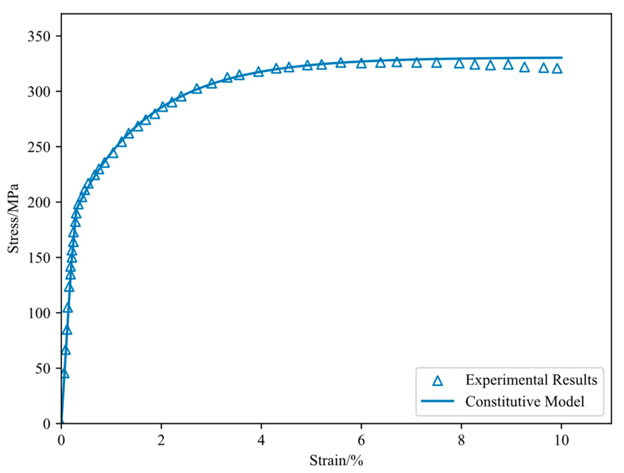
The parameters of the constitutive and damage evolution models are calibrated using the least square method. In the constitutive model, C k and γ k are calibrated with uniaxial tension test results from Zhang et al. [42], and the result, the stress–strain curve, is shown in Figure 2. The uniaxial tension results for the three building directions are very similar to each other, and the parameters are calibrated with the curve for 0° built specimens. Results are presented in Table 1.
In the fatigue damage model, parameters are calibrated with fatigue strength evaluation results and fatigue life test results. First, integrate Equation (14) from D = 0 to D = 1 :
N F = a r e a θ a r e a 0 γ 1 1 + β 1 α M 0 β     σ u σ m a x σ a σ l 0 1 b 1 σ m σ a 1 b 2 σ m β  
where N F is the loading cycle for crack initiation, a r e a is derived from fractural mechanics analysis in [42], β , α M 0 β , b 1 , b 2 and γ are derived from fatigue life test results.
Next, with α M 0 β and β available, a test run of FE calculation detailed in Section 3.3 is carried out with different combinations of α and M 0 . The calculation results are compared to fatigue test data to determine the final value of these two parameters. Note that γ = 1 for specimens built with 0° direction, which is used as a reference here. Results are shown in Table 2.

3.2. Finite Element Implementation of Theoretical Model

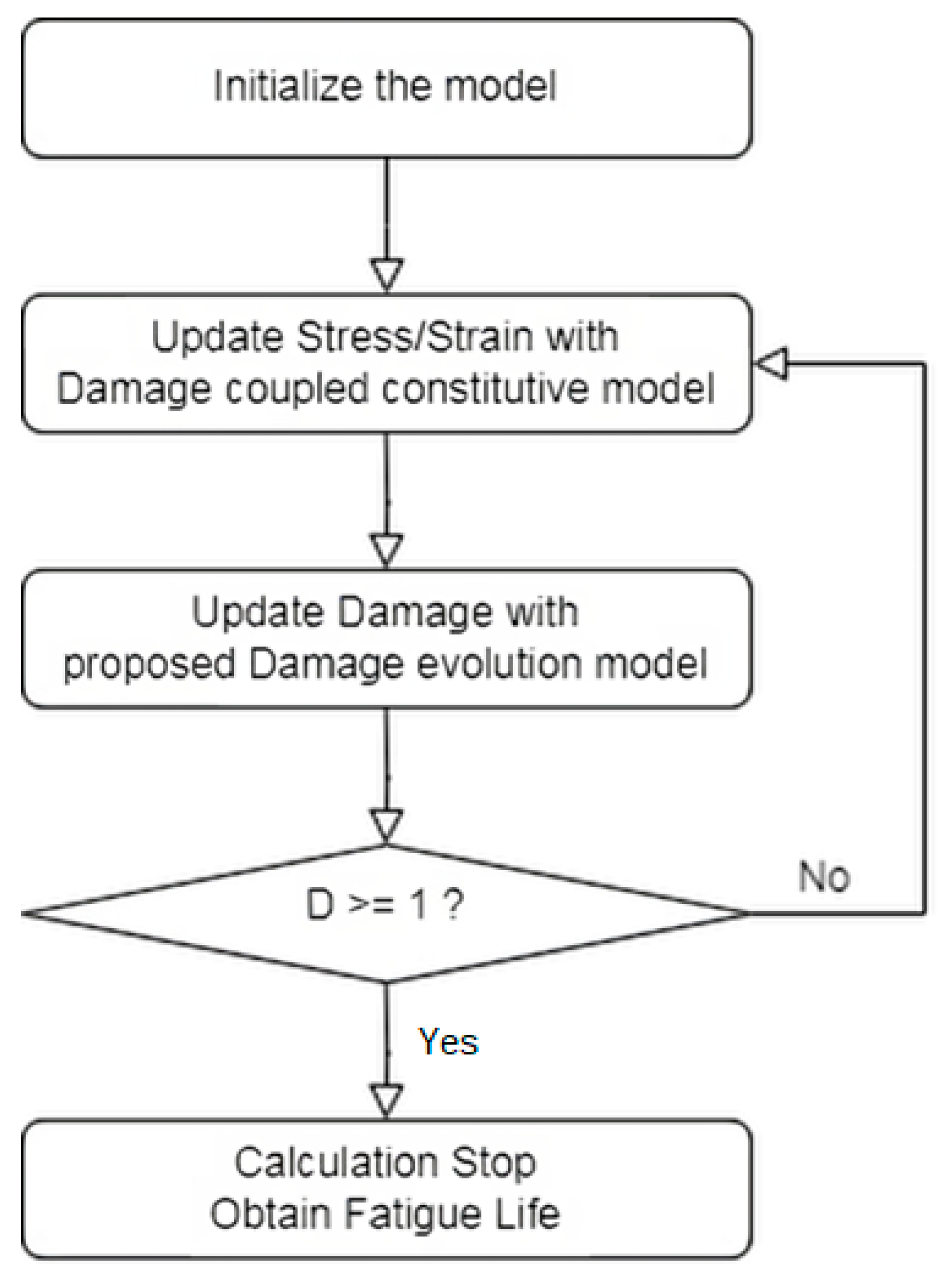
Based on the proposed models, this paper implements a continuum damage mechanics-based finite element (CDM-FE) numerical method by developing custom user material and user subroutines in the ABAQUS platform. The method is as follows:
1.
Initialize the model and variables, such as damage variable D and fatigue life N F ;
2.
Apply cyclic loading and update the elastic modulus based on the accumulated fatigue damage;
3.
Calculate the stress–strain distribution at each integration point of the FE model with the damage-coupled constitutive model;
4.
Calculate and update the damage rate d D / d N at each integration point according to the proposed damage model. To save computational time, assume that the damage accumulation is linear in Δ N cycles. The damage increment will be ( d D / d N ) Δ N , and is updated at each integration point;
5.
Check if damage at any integration point exceeds 1. If so, terminate the calculation and output the fatigue life. Otherwise, return to step 2 and repeat. It is clear from Equation (3) that the elastic modulus of the material will drop to 0 once the damage exceeds 1, and this is considered crack initiation.
Figure 3 describes the above procedure in a flowchart.

3.3. CDM-Based Numerical Results

The proposed model is validated against fatigue test data from Zhang et al. [42]. The specimens Zhang et al. tested are built with a laser power of 330 W, a scan speed of 1700 mm/s, a layer thickness of 0.03 mm, and a scan span of 0.15 mm. The built cylinder parts are annealed at 270 °C for stress relief for 2 h, washed with acid, and machined into the final fatigue test specimens.
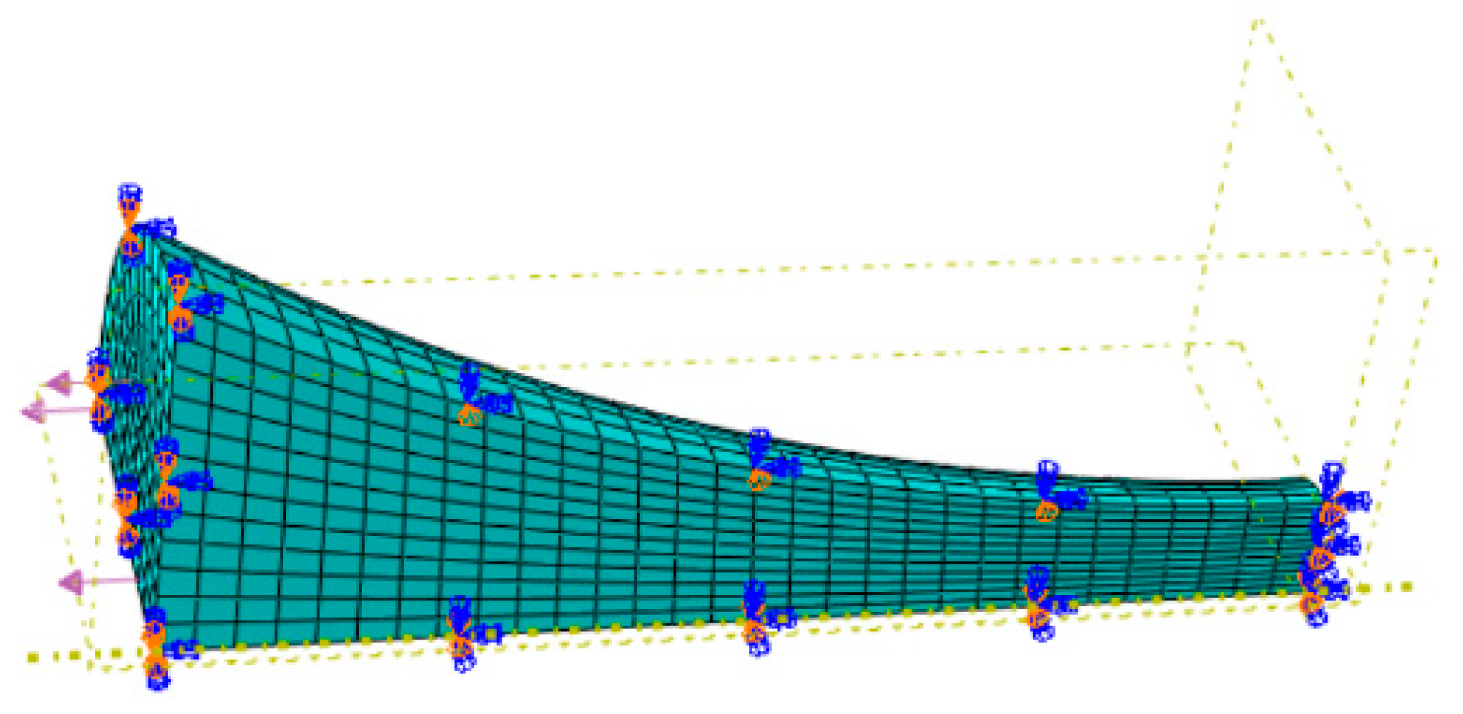
A one-eighth FE model of the cylinder specimen is built for calculation, considering the axial symmetry of the specimen. The length between the two faces is 20 mm, and the necking face and end face are disks with radii of 4 mm and 7 mm, respectively, as shown in Figure 4. The cyclic load is applied to the end of the specimen, and three symmetric constraints are applied on each corresponding symmetrical plane, as shown in Figure 5.
There are 3937 nodes and 3240 C3D8 elements in this model, and the smallest size of elements is 0.17 by 0.17 by 0.67 (mm). The analysis is carried out with the ABAQUS/Standard implicit solver, and the stress convergence is verified with two sets of denser meshes, the results are shown in Table 3. The von Mises stress is measured at the same critical point across three sets of meshes. The original mesh adopted in this paper exhibits good accuracy and is able to strike a balance between numerical accuracy and computational time.
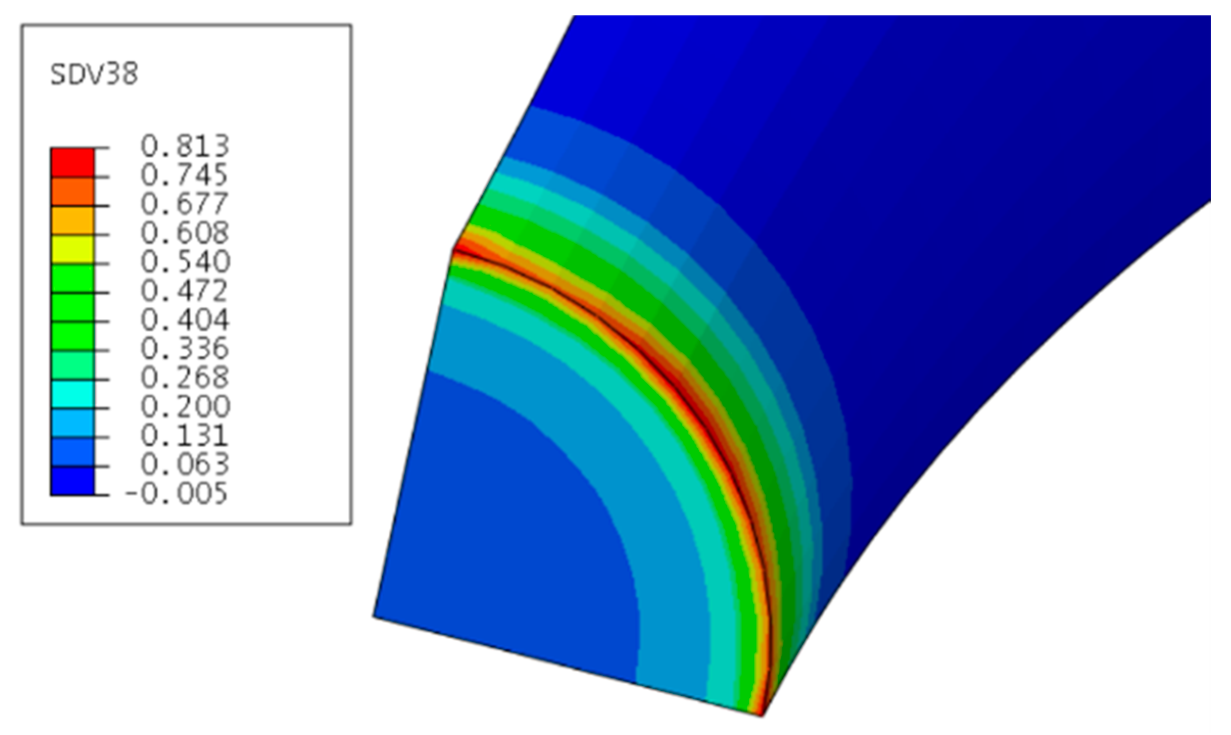
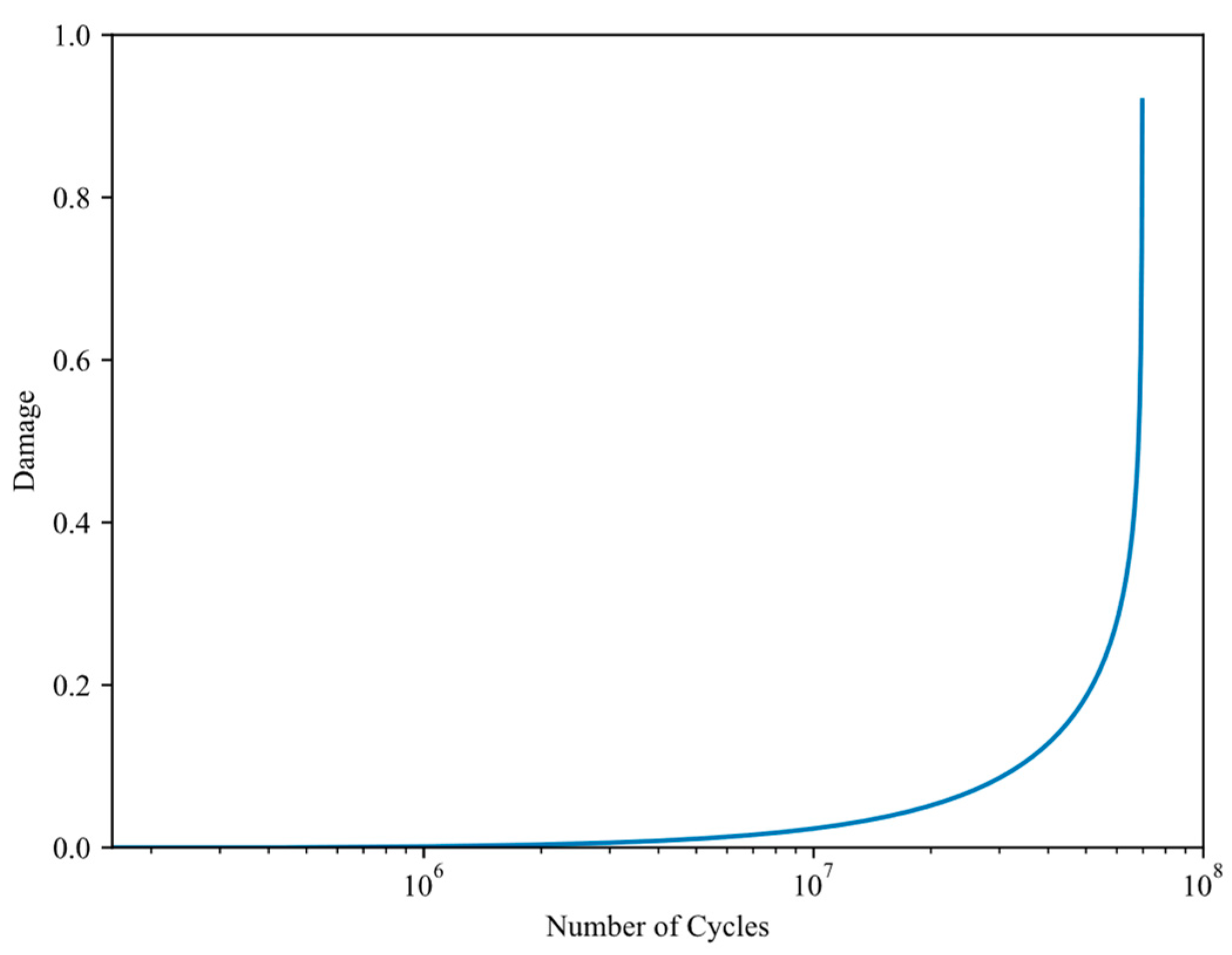
The damage distribution of a specimen built with 0° direction under σ a = 150 MPa and R = 0 is shown in Figure 6. The maximum damage is observed at the minimum cross-section. The damage evolution at the critical point over the number of cycles is plotted in Figure 7. The damage accumulation initially increases slowly and increases rapidly in the last 20% of the fatigue life. Since the damage accumulation is equivalent to elastic modulus degeneration in an RVE, under a constant stress level, the damage variable increases in a positive feedback manner.
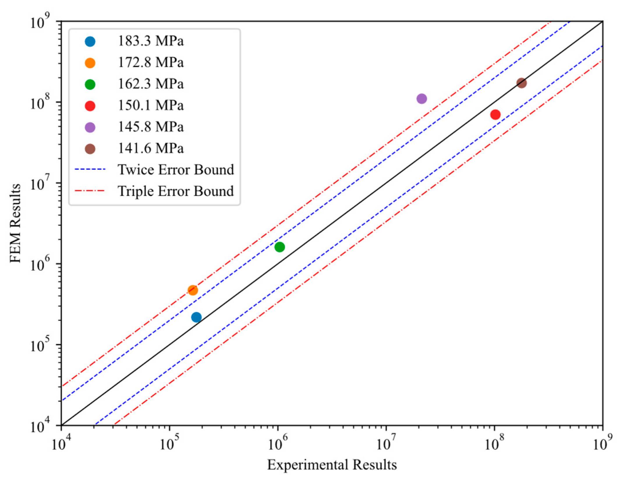
The predicted fatigue lives of SLM AlSi10Mg specimens built with 0° are presented in Figure 8. The majority of predicted results fall within the triple error bound. This validates the CDM-FE numerical method and the calibrated material parameters. It is noteworthy that the σ a = 145.8 MPa experimental fatigue life is shorter than that of σ a = 150.1 MPa. This further demonstrates that internal defects play an important role in the fatigue and damage evolution process.
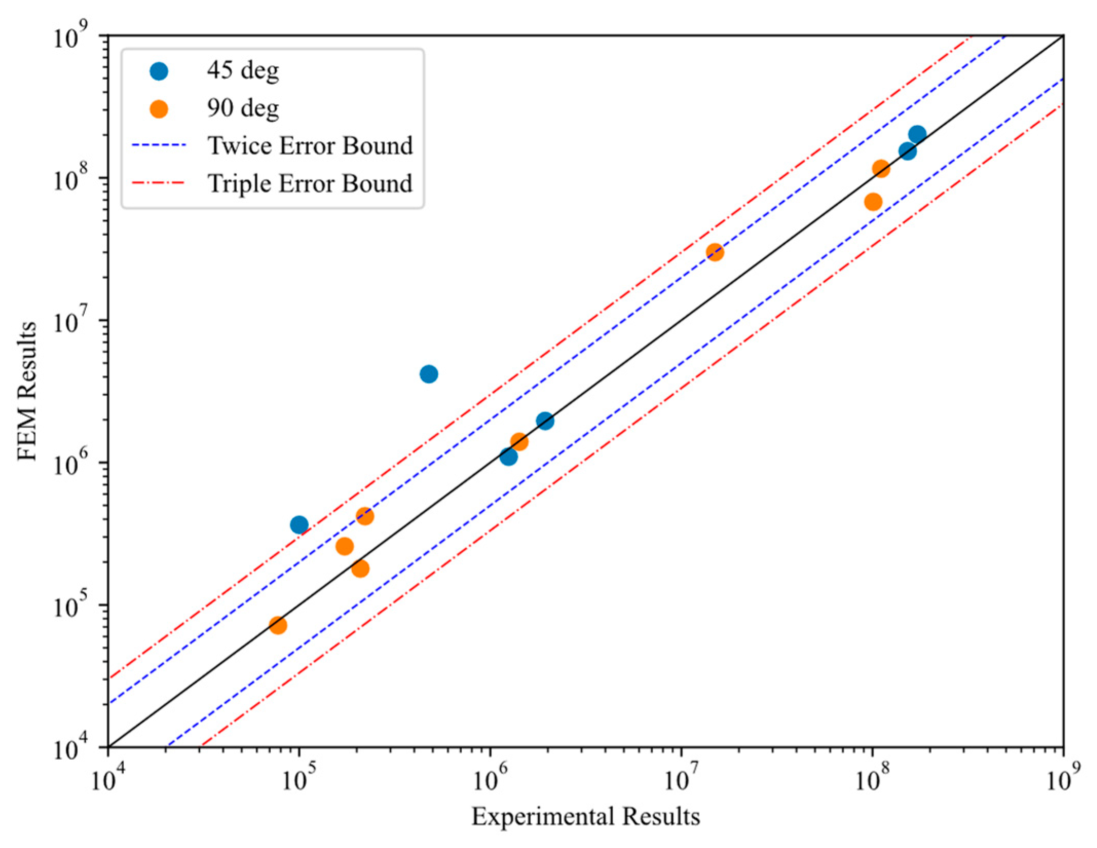
For the specimens built with 45 and 90° direction, the results are shown in Figure 9. Like 0° results, the majority of predictions are within the triple error band. This further validates the applicability of the proposed model.

4. A Machine Learning Approach for SLM AlSi10Mg VHCF Life Prediction

Before the machine learning process, the collected data need to be preprocessed to improve the accuracy and reliability of the prediction results. Typical data pre-process consists of four different steps:
1.
Data Cleaning: This step removes inconsistencies from the original data, such as missing values and duplicate records. These inconsistencies can prevent the model from accurately reading the data. Typically, the entries with missing values are removed from the dataset.
2.
Data Transformation: This step converts the data into a format that is convenient for programming and models to understand. This process often includes dimension reduction.
3.
Data Splitting: This step splits the data into two or more sets, each set with a different purpose. Typically, data are split into two parts, a training set and a test set. The model is trained on the training set and tested on the test set. This helps avoid overfitting and tests the ability of the model to process unseen data.
4.
Data Normalization: This step normalizes the data to a certain range. This helps speed up the learning process. Typically, data are normalized to have a mean of zero and a deviation of one.

4.1. Support Vector Machine and Support Vector Regression

Support vector machine (SVM) is a machine learning algorithm for classification and regression tasks. The regression variant is also known as support vector regression (SVR). SVM utilizes several support vectors to define the final model, and as a result, SVR is very memory efficient and fast compared to other ML models. Utilizing support vectors also makes SVR relatively robust to outliers. With a kernel function, SVR is also able to handle non-linear relationships. However, under extreme conditions, the choice of kernel functions becomes crucial for results to be reliable.
Consider a plane P and a dataset D = x 1 , y 1 , x 2 , y 2 , , x n , y n where y i { 1 , 1 } for all i scattered on P . SVM finds a line L (or a hyperplane in higher dimensions) w T x + b = 0 to divide P into two parts so that only one kind of data (namely, y i = 1 or 1 ) lies on each part of the plane. The distance r between points in D and L is:
r = w T x + b | w |  
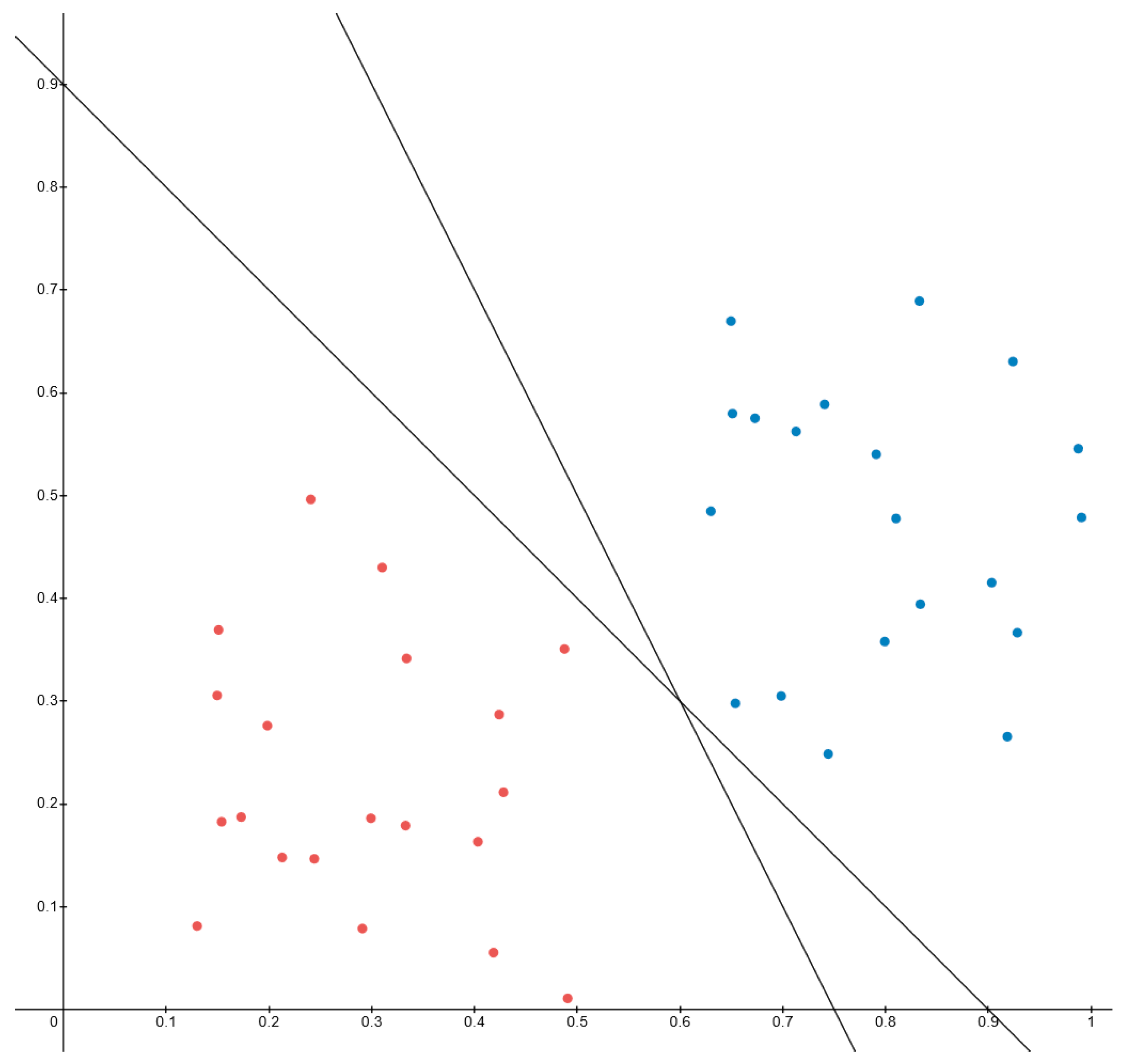
In general, more than one L is feasible to divide P , as shown in Figure 10. In this case, taking account into unseen data, the best L should be the one furthest from both group of points. Points that are the closest to L in each group are called the support vectors of L . The sum of the distance between two support vectors in different groups to L is called the margin of L . If we scale down w and b so that for support vectors, r s v = 1 , then the margin is defined as:
γ = 2 | w |  
The goal of SVM is to find the optimal L that maximizes the margin by changing w and b . This can be formulated as the following problem:
max w , b 2 | w |   s . t .   y i w T x i + b 1 ,   i = 1,2 , , m
Noticing that maximize w 1 is the same as minimize w 2 , we substitute 2 / w with w 2 / 2 , apply Lagrange multiplier to find its dual problem:
L w , b , λ = 1 2 w 2 + i = 1 m λ i 1 y i w T x i + b
Solve L w = 0 and L b = 0 , we get
w = i = 1 m λ i y i x i
0 = i = 1 m λ i y i
Substitute Equations (20) and (21) into (19), we get the final dual problem:
Λ = max λ i = 1 m λ i 1 2 i = 1 m j = 1 m λ i λ j y i y j x i T x j ,   s . t .   i = 1 m λ i y i = 0 ,   λ i 0 ,   i = 1,2 , , m
Solve Λ λ = 0 , and we get the best L with the largest margin:
L = w T x + b = i = 1 m λ i y i x i T x + b
We then utilize algorithms like sequential minimal optimization (SMO) to solve for λ i and obtain b from all support vectors:
b = 1 S s S ( 1 y s i S λ i y i x i T x s ) ,   S = { i | λ i > 0 ,   i = 1,2 , , m }
We now revisit the original problem Equation (18), which is restrained by inequalities, and must satisfy the Karush–Kuhn–Tucker (KKT) conditions. The KKT conditions for this problem are λ i 0 , y i w T x i + b 1 0 and λ i y i w T x i + b 1 = 0 , where i = 1,2 , , m . The last constraint implies that for any ( x i , y i ) D , either λ i = 0 or y i w T x i + b = 1 . This means for any points in D that are not support vectors of L can be discarded without affecting the results.
SVR works similarly to SVM, but usually with a tolerance of an error ε between the real value Y and the predicted value y , or in ML terms, the loss function will not grow when Y y ε . The problem is:
max w , b 2 | w | + C i = 1 m r ( y i Y i ) ,   i = 1,2 , , m
where C is a punishment parameter, r is the distance between y and Y offset by the tolerance. If Y y ε , r = 0 , else r = Y y ε .
We then introduce two slack variables ξ i and ξ i ^ to the problem. Like SVM, we solve partial derivatives and apply KKT constraints. The final dual problem is
max λ i , λ i ^ i = 1 m y i λ i ^ λ i ε λ i ^ + λ i 1 2 i = 1 m j = 1 m λ i ^ λ i λ j ^ λ j x i T x j   s . t .   i = 1 m λ i ^ λ i = 0 ,   0 λ i , λ i ^ C
Similarly, we utilize sequential minimal optimization SMO to solve for λ i , λ i ^ . The SVR solution is given by
y = i = 1 m λ i ^ λ i x i T x + b ,   b = y i + ε j = 1 m λ j ^ λ j x j T x j
However, unlike the example shown in Figure 10, real-life problems are not always linearly separable. We introduce kernel functions to map the data to higher dimensional spaces, where the data may become linearly separable. A widely used kernel function is the radial basis function (RBF):
K x i , x j = exp ( γ x i x j 2 )
where γ is a parameter of RBF.

4.2. SVR Parameter Calibration with PSO and Training

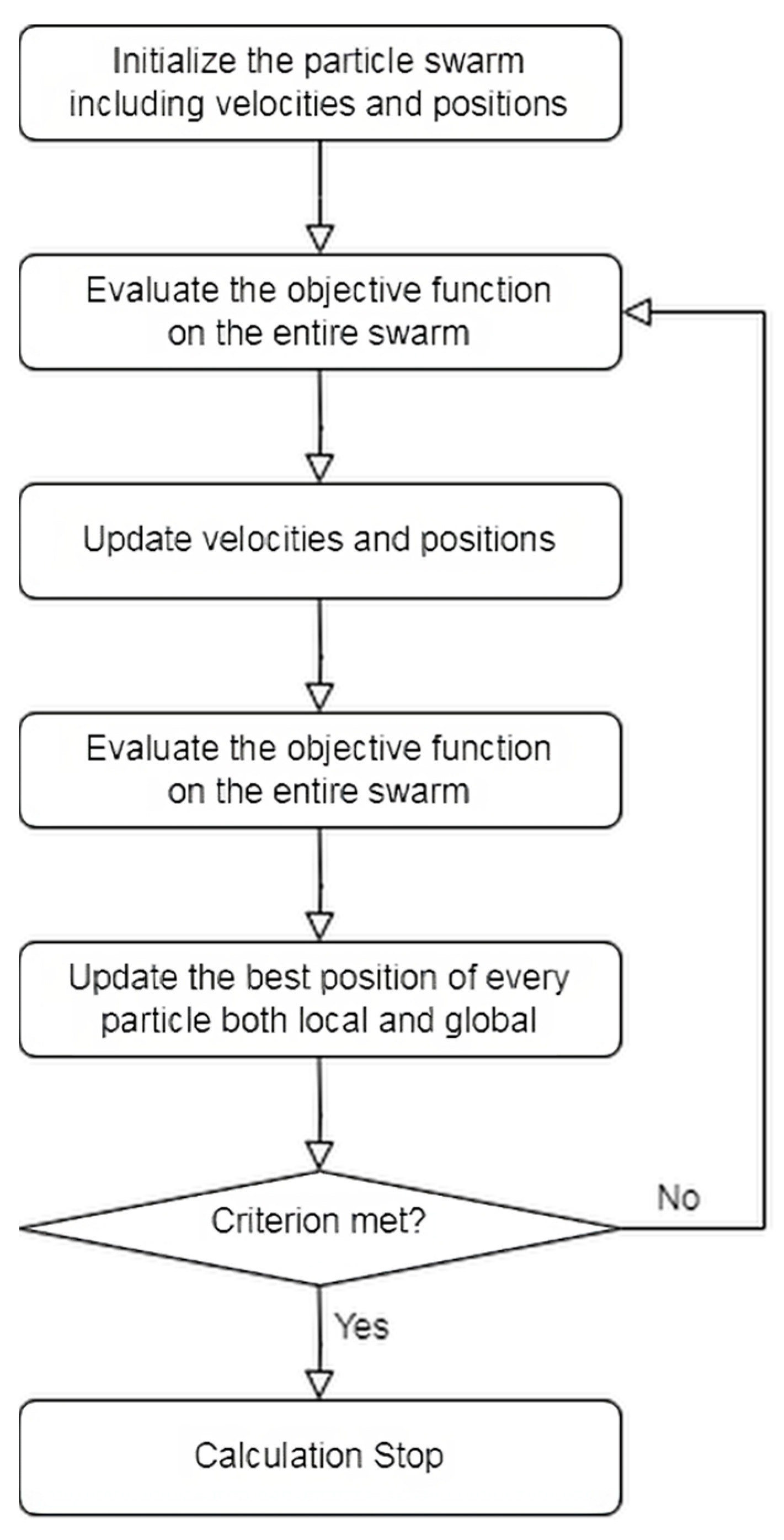
We utilize particle swarm optimization (PSO) to calibrate parameters. First, a set of particles are deployed into a search space, where they are able to roam around. Each particle has a position and a velocity, and these parameters are updated every iteration, based on both the best-known position of itself and its neighbors. The goal is to slowly adjust the velocity of each particle and guide them toward the global optimum in the search space. A typical PSO procedure is as follows:
1.
Initialize the search space with particles randomly distributed through the search space;
2.
Evaluate the objective function for each particle;
3.
Update the velocity of particles based on the evaluation results of itself and its neighbors for each particle;
4.
Reevaluate the objective function for each particle;
5.
Compare the evaluation results in step 4 to the best-known positions of each particle and update if necessary;
6.
Determine the best particle based on the evaluation results in step 4;
7.
Repeat steps 3–6 until the criterion is met or the global optimum is found.
Figure 11 describes the above procedures in a flowchart.
The parameters to be calibrated are C , ε and γ . We combine PSO with SVR training progress to determine the results on the fly, every update of every particle corresponds to an SVR training process. The Pearson correlation coefficient is utilized to evaluate the fitness between SVR predictions and CDM-FE predictions.
The database consists of real experimental results and CDM-FE predictions, in total, 100 tuples of data {direction, stress, life}. This is further randomly divided into two parts by a program, 82% as the training set, and the remaining 18% as the test set. The SVR model is trained on the training set and then evaluated on the test set to avoid overfitting and test its ability against unseen data.
The parameters calibrated with PSO are C = 3100 , γ = 10 5 and ε = 5 × 10 5 .

4.3. SVR-CDM Based Predictions

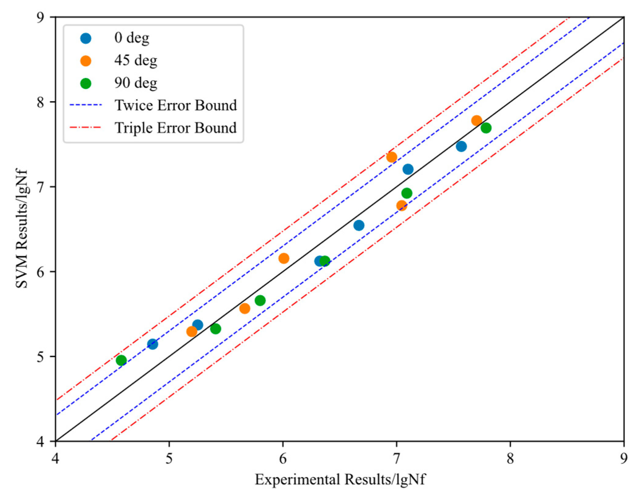
Figure 12 shows the performance of the trained SVR model on the test set. Compared to Figure 8 and Figure 9, all predictions are within the triple error bound, and SVR prediction results are generally closer to experimental results than CDM-FE prediction results. To quantify the difference, we calculate the root mean square error (RMSE), the mean absolute error (MAE) and R 2 score, as shown in Equation (29)–(31), for SVR group and CDM-FE group. RMSE and MSE indicate the overall spread of the predictions y i around the true values Y i . Lower RMSE usually indicates less spread around true values, and thus, a better fit. MAE also measures the overall spread, but different from RMSE and MSE, every difference is weighted equally, so large errors are less influential. R 2 ranges from 0 to 1, higher values indicate a better fit. RMSE, MAE and R 2 are defined as follows:
R M S E = 1 m i = 1 m Y i y i 2
M A E = 1 m i = 1 m | Y i y i |
R 2 = 1 i = 1 m Y i y i 2 i = 1 m y ¯ y i 2
where Y i are the real values (the experimental results) and y i are predicted values (predicted by the models). We choose RMSE here instead of regular MSE because the fatigue life results are usually in the range of 10 5 ~ 10 7 ; thus, the results of MSE will be in the range of 10 10 ~ 10 14 , which is too large and not convenient for comparison.
The RMSE, MAE and R 2 values of SVR predictions and CDM-FE predictions are shown in Table 4.
We can see that compared to the CDM-FE approach, the SVR method is better at both the spread and the fitness with respect to experimental results. The overall prediction accuracy of SVR is better than that of the CDM-FE model.

5. Discussion

Some data in this section are obtained with the CDM-FE numerical method, combined with the calibrated parameters. In Section 5.1, the damage evolution with a fixed stress level under different building directions is calculated with the CDM-FE method. In Section 5.2, the damage evolution at a certain stress level with different stress ratios and the damage evolution under different stress levels with a certain stress ratio and build direction are calculated and compared with the CDM-FE method. In Section 5.3, the effect of the parameters of SVR on the prediction accuracy is studied.

5.1. Influence of Building Direction on the Fatigue Life

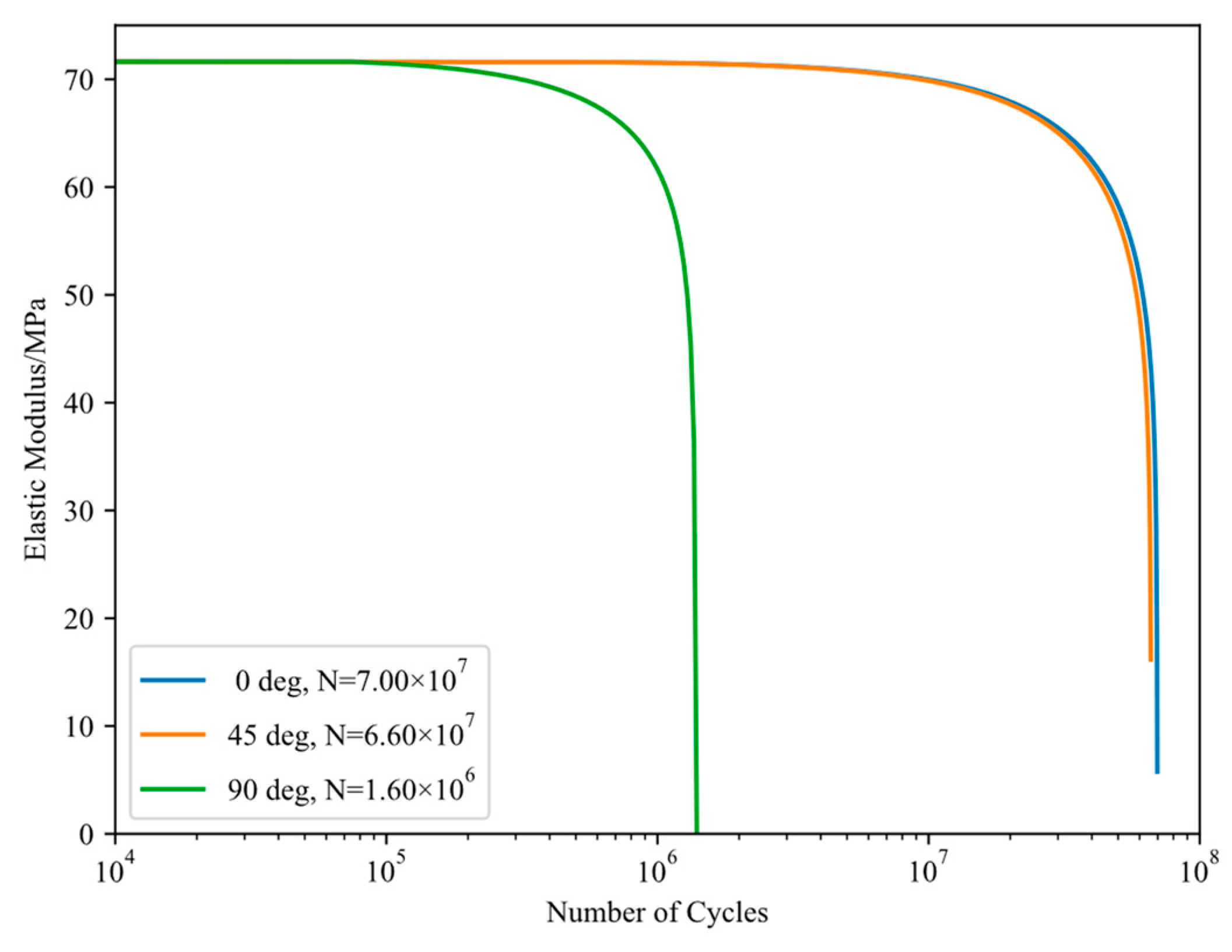
From previous research and the model validating process, we can clearly see that as the build direction decreases, the damage evolution slows down, resulting in a longer fatigue life. The calculation is carried out under R = 0 , σ a = 150 MPa, and the results are shown in Figure 13. The results of 0° and 45° are similar and are both significantly longer than 90°. This agrees with previous research results we have seen earlier. The variation of elastic modulus is shown in Figure 14. We can see that as the damage accumulates, the elastic modulus of the material degrades before the material finally fails. The rapid growth of damage only accounts for about 20% of the whole process of damage evolution.

5.2. Influence of Stress Ratio and Stress Level on the Damage Accumulation and Evolution Rate

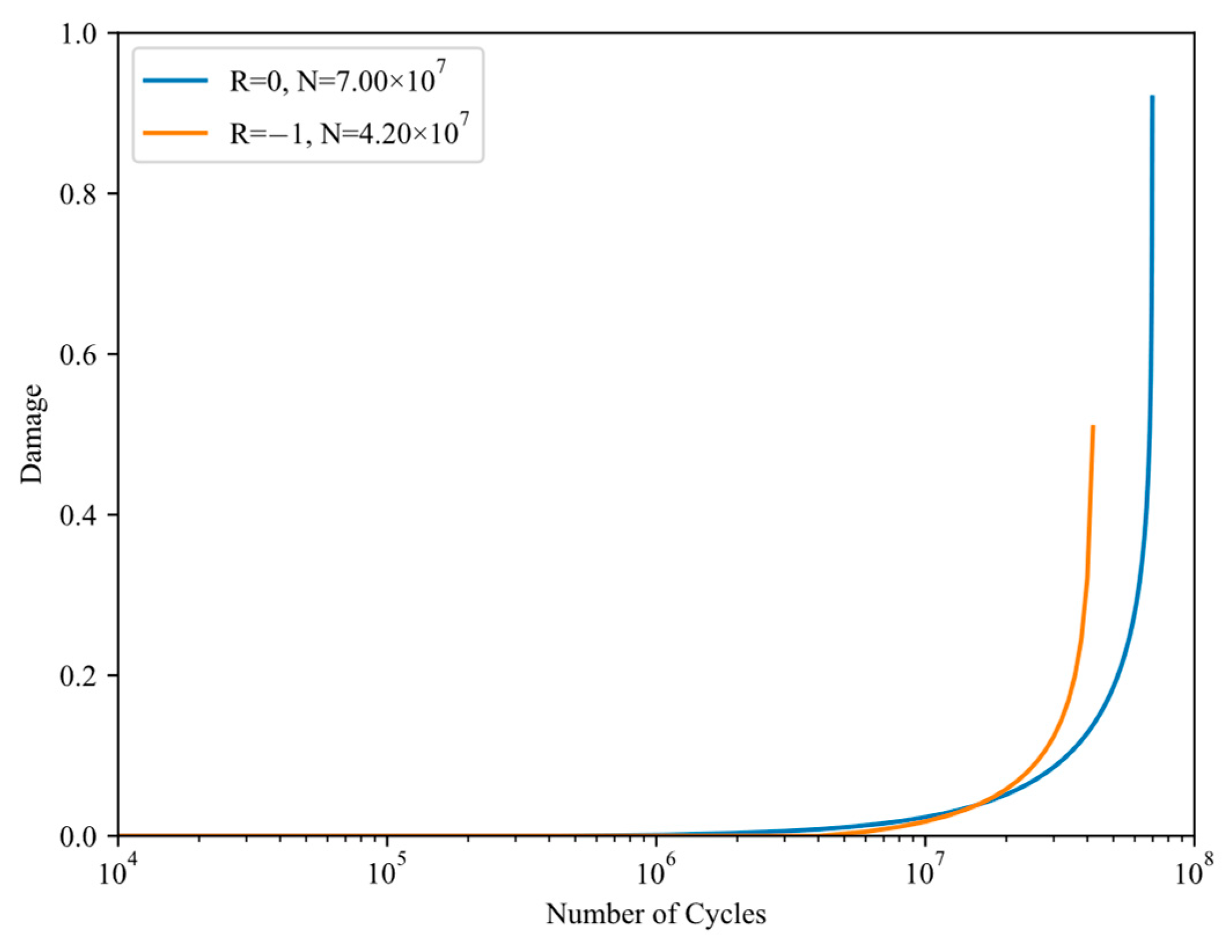
Under the fixed stress level σ a = 150 MPa and build direction = 0°, we compare the damage evolution under different stress ratios. Results are shown in Figure 15. We can see as the stress ratio R decreases from 0 to −1, the related damage evolution accelerates, resulting in a shorter fatigue life. With build direction kept at 0° and stress ratio R = 0 , we then calculate the damage evolution under different stress levels. The damage evolution clearly accelerates with higher stress levels, leading to a shorter fatigue life, as shown in Figure 16. However, in the previous experimental results, we saw that the experimental fatigue life under σ a = 145.8 MPa is actually shorter than that under σ a = 150.1 MPa. This suggests that the stress level is only one factor affecting the fatigue process, and although our model considers the effect of the internal defect by taking the characteristic length of the defect into account, the location of the defect in the material matrix will also affect the final experimental results.

5.3. Influence of SVR Parameters on the Prediction Accuracy

In this section, the influence of SVR parameters on the prediction accuracy of SVR is studied. RMSE function is employed to measure the accuracy. Figure 17 shows the effects of different penalty parameters C ranging from 100 to 100,000. We can see a the RMSE of the model has a local minimum at around C = 5000 , and it increases again after this. The model is penalized by increasing the value of the loss function when related constraints are violated. As suggested in Equation (25), the first term aims to maximize the margin, while the second term aims to minimize the distance. These two constraints are conflicting, thus depending on the value of C , one term will be dominant over the other one. When C is large enough, the other term will be negligible, and vice versa. These conditions effectively destroy one of the two constraints, thus degrading the prediction accuracy.
Figure 18 shows the effect of different tolerance parameters ε ranging from 0 to 0.01. We can see a local minimum at around 0.3 and RMSE first decreases then increases as ε increases. The tolerance parameter determines how far away data points can be from L before increasing the value of the loss function. If constrained too strictly or too loosely, the prediction accuracy will suffer.
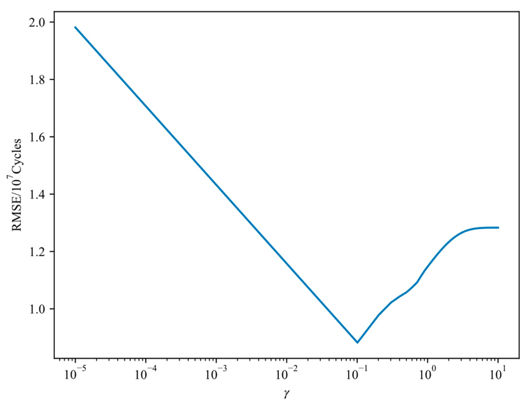
Figure 19 shows the effect of different kernel parameters γ ranging from 1 × 10⁻⁵ to 1. We can see a local minimum around γ = 0.09 and RMSE first decreases and then increases as γ increases. The kernel parameter is a parameter utilized in the kernel function of SVR to map the input data to a higher dimensional space, making the data easier to be divided and, thus, easier to find L . Like ε , if constrained too strictly or too loosely, the prediction accuracy will suffer.

6. Conclusions

In this paper, a novel VHCF model considering the effect of defect size and AM building direction in SLM AlSi10Mg is proposed. The research presents a damage-coupled constitutive model and a novel fatigue damage model. These models are implemented by developing user custom materials and user subroutines with ABAQUS. The resulting predictions for SLM ALSi10Mg under different build directions fall within the triple error bound, and this validates the proposed implementation method and material parameters.
An SVR-based ML model is also proposed to predict the fatigue life of SLM AlSi10Mg. The model is trained on both experimental results and CDM-FE calculation results, and the prediction is compared to CDM-FE method. The SVR model gives an overall higher R 2 value and lower RMSE/MAE, indicating that the prediction given by the SVR model is superior to that of the CDM-FE method.
Additionally, it is observed that under the same stress level and stress ratio, a smaller build direction has a longer fatigue life than a larger build direction. Additionally, higher stress levels and lower stress ratios contribute to faster damage evolution, thus a shorter fatigue life. The effect of SVR parameters on the prediction accuracy is also discussed.
This study offers another perspective and a set of tools for understanding the VHCF behavior of SLM AlSi10Mg. However, the proposed model fails to take certain factors into account, such as the distribution of internal effects. Moreover, the lack of available experimental data limits the accuracy of the proposed model. Future research will address these limitations and consider other influencing factors, as well as enhancement of the model’s performance in terms of prediction accuracy.

Author Contributions

Conceptualization, Y.Y. and L.S.; Methodology, L.S. and C.S.; Software, Y.Y.; Validation, L.S. and X.W.; Formal Analysis, W.H. and Y.Y.; Investigation, W.H., Z.Z. and X.C.; Resources, Z.Z., L.S. and Z.B.; Data Curation, Y.Y.; Writing—Original Draft Preparation, Y.Y., L.S., Z.Z., X.W. and W.H.; Writing—Review and Editing, Z.Z., C.S., Z.B., W.H. and X.C.; Visualization, W.H.; Supervision, Z.Z. and X.C.; Project Administration, Z.Z. All authors have read and agreed to the published version of the manuscript.

Funding

This research was funded by the scientific research project of China Academy of Railway Sciences Co., Ltd. (2021YJ069) and the Natural Science Foundation of China (52178441).

Data Availability Statement

Not applicable.

Acknowledgments

Xiao Chen sincerely acknowledges the support from the Postdoctoral International Exchange Program (funded by the China Postdoc Council).

Conflicts of Interest

The authors declare no conflict of interest.

Nomenclature

D damage variable
E Young’s modulus
ε i j total strain
ε i j e elastic strain
ε i j p plastic strain
σ i j stress component
R v triaxial stress function
ν Poisson’s ratio
δ i j Kronecker delta
Y damage strain energy density release rate
Ψ Helmholtz free energy
σ e q von Mises equivalent stress
C k , γ k material parameters of constitutive model
σ a amplitude of a loading cycle
σ m mean stress of a loading cycle
α , β , M 0 , b 1 , b 2 material parameters of damage evolution model
A I I octahedral shear stress amplitude
σ H , m mean hydrostatic stress
σ e q , m a x maximum of von Mises equivalent stress
σ u yield stress
σ l 0 fatigue limit
s i j , m a x , s i j , m i n maximum and minimum of the deviatoric stress tensor in a loading cycle
N F initiation life
R stress ratio
X input data
Y i experimental data
y i predicted data
AMadditive manufacturing
SLMselective laser melting
CDMcontinuum damage mechanics
SVMsupport vector machine
SVRsupport vector regression
FEfinite element
PSOparticle swarm optimization

References

  1. Wang, H.M. Materials’ fundamental issues of laser additive manufacturing for high-performance large metallic components. Acta Aeronaut. Astronaut. Sin. 2014, 35, 2690–2698. [Google Scholar]
  2. Liu, Q.; Lu, B.H. Review on Quality Control and Relevant Hybrid Technology in Additive Manufacturing of Metallic Materials. Mater. Rep. 2024, 1–15. Available online: http://kns.cnki.net/kcms/detail/50.1078.TB.20230410.1937.051.html (accessed on 19 April 2023).
  3. Sola, A.; Nouri, A. Microstructural porosity in additive manufacturing: The formation and detection of pores in metal parts fabricated by powder bed fusion. J. Adv. Manuf. Process. 2019, 1, e10021. [Google Scholar] [CrossRef]
  4. Lu, H.F.; Lv, J.M.; Luo, K.Y.; Lu, J. Microstructure and Mechanical Properties of Ti6Al4V Alloy by Laser Integrated Additive Manufacturing with Alternately Thermal/Mechanical Effects. Acta Metall. Sin. 2023, 59, 125–135. [Google Scholar]
  5. Zhang, W.Q.; Zhu, H.H.; Hu, Z.H.; Zeng, X. Study on the selective laser melting of AlSi10Mg. Acta Metall. Sin. 2017, 53, 918–926. [Google Scholar]
  6. Zhang, X.; Liu, S. Aerocraft aluminum alloys and their materials processing. Mater. China 2013, 32, 39–55. [Google Scholar]
  7. Li, S.; Fu, G.; Li, H.; Peng, Q.; Xiao, H.; Zhang, J.; Zhang, Z. Research Progress on Absorptivity of Selective Laser Melting Additive Manufacturing. Mater. Rep. 2023, 1–24. Available online: http://kns.cnki.net/kcms/detail/50.1078.tb.20230206.1618.001.html (accessed on 19 April 2023).
  8. Tan, Y.; Zhang, Y.; Lu, B.; Yan, X.; Li, Y.; Dai, M.; Liu, M. High Temperature Hardness and Oxidation Behavior of TiAl Alloy Fabricated by Electron Beam Selective Melting Additive. Rare Met. Mater. Eng. 2023, 52, 222–229. [Google Scholar]
  9. Zhang, Z.; Zeng, Q.; Liu, L.; Sun, C. Forming regularity of aluminum alloy formed by laser induced MIG arc additive manufacturing. Trans. China Weld. Inst. 2019, 40, 7–12. [Google Scholar]
  10. Zhang, G.; Zhang, P.; Gao, J.; Yu, H.; Yuan, H.; Ding, Y.; Xiong, H. Microstructure and Mechanical Properties of TC11 Titanium Alloy Fabricated by Wire-feed Electron Beam Additive Manufacturing. J. Mech. Eng. 2023, 1–8. Available online: http://kns.cnki.net/kcms/detail/11.2187.TH.20230202.1604.011.html (accessed on 19 April 2023).
  11. Ying, W.; Han, F. Oxidation Behavior and Control of Rene 104 Superalloy Produced by Laser Solid Forming. Electromach. Mould. 2018, 31, 39–44. [Google Scholar] [CrossRef]
  12. Ao, N.; He, Z.; Wu, S.; Peng, X.; Wu, Z.; Zhang, Z.; Zhu, H. Recent progress on the mechanical properties of laser additive manufacturing AlSi10Mg alloy. Trans. China Weld. Inst. 2022, 43, 1–19+113. [Google Scholar]
  13. Wang, K.; Jiao, X.; Zhu, J.; Li, J.; Du, S. Effect of laser power density on wear resistance of TC4 alloy manufactured by SLM. Trans. China Weld. Inst. 2020, 41, 61–64. [Google Scholar]
  14. Fiegl, T.; Franke, M.; Koerner, C. Impact of build envelope on the properties of additive manufactured parts from AlSi10Mg. Opt. Laser Technol. 2019, 111, 51–57. [Google Scholar] [CrossRef]
  15. Aboulkhair, N.T.; Everitt, N.M.; Ashcroft, I.; Tuck, C. Reducing porosity in AlSi10Mg parts processed by selective laser melting. Addit. Manuf. 2014, 1, 77–86. [Google Scholar] [CrossRef]
  16. Thijs, L.; Kempen, K.; Kruth, J.P.; Van Humbeeck, J. Fine-structured aluminium products with controllable texture by selective laser melting of pre-alloyed AlSi10Mg powder. Acta Mater. 2013, 61, 1809–1819. [Google Scholar] [CrossRef]
  17. Wu, H.H.; Li, J.F.; Wei, Z.Y.; Wei, P. Effect of processing parameters on forming defects during selective laser melting of AlSi10Mg powder. Rapid Prototyp. J. 2020, 26, 871–879. [Google Scholar] [CrossRef]
  18. Cai, X.; Dong, B.; Yin, X.; Lin, S.; Fan, C. Influences of pre-heating temperatures on the microstructures and mechanical properties of GTA additive manufactured TiAl based alloy. Trans. China Weld. Inst. 2021, 42, 14–21. [Google Scholar]
  19. Jian, Z.M.; Qian, G.A.; Paolino, D.S.; Tridello, A.; Berto, F.; Hong, Y.S. Crack initiation behavior and fatigue performance up to very-high-cycle regime of AlSi10Mg fabricated by selective laser melting with two powder sizes. Int. J. Fatigue 2021, 143, 106013. [Google Scholar] [CrossRef]
  20. Larrosa, N.O.; Wang, W.; Read, N.; Loretto, M.H.; Evans, C.; Carr, J.; Tradowsky, U.; Attallah, M.M.; Withers, P.J. Linking microstructure and processing defects to mechanical properties of selectively laser melted AlSi10Mg alloy. Theor. Appl. Fract. Mech. 2018, 98, 123–133. [Google Scholar] [CrossRef]
  21. Wu, Z. Evaluation of Anisotropic Fatigue Performance of Additively Manufactured Aluminum Alloy Based on 3D X-ray Computed Tomography of Defects. Ph.D. Thesis, Southwest Jiao-Tong University, Chengdu, China, 2020. [Google Scholar]
  22. Xu, Z.W.; Liu, A.; Wang, X.S. Fatigue performance and crack propagation behavior of selective laser melted AlSi10Mg in 0°, 15°, 45° and 90° building directions. Mater. Sci. Eng. A 2021, 812, 141141. [Google Scholar] [CrossRef]
  23. Zhao, X.; Lu, G.; Peng, X.; Zhang, N.; Qin, J. Fatigue life prediction of complex aeronautical components based on damage mechanics. Chin. J. Appl. Mech. 2020, 37, 1007–1012+1386–1387. [Google Scholar]
  24. Wu, L.; Wang, R.; Liu, F.; Qin, Q.; Chang, Y.; Wang, Z. Fatigue life prediction of resistance spot welded joints of AZ31B/TA15 dissimilar materials. Trans. Mater. Heat Treat. 2022, 43, 168–176. [Google Scholar]
  25. Zhang, S.; Wu, H. Life Evaluation of Multiaxial Variable Amplitude Low-Cycle Fatigue Based on Sequential Rain flow Method and Critical Plane Method. Chin. Q. Mech. 2020, 41, 465–476. [Google Scholar] [CrossRef]
  26. Zhang, D. Fatigue Life Prediction of High Strength Steel Welds under Prestrain Based on Energy Method and Its Application. Ph.D. Thesis, Hunan University of Technology, Hunan, China, 2022. [Google Scholar] [CrossRef]
  27. Shao, Q. Numerical Simulation of Fatigue Crack Propagation of Brittle Fracture Based on Phase Field Method. Ph.D. Thesis, Southwest Jiaotong University, Chengdu, China, 2019. [Google Scholar] [CrossRef]
  28. Gao, T.; Tong, Y.; Zhan, Z.; Mei, W.; Hu, W.; Meng, Q. Development of a non-local approach for life prediction of notched specimen considering stress/strain gradient and elastic-plastic fatigue damage. Int. J. Damage Mech. 2022, 31, 1057–1081. [Google Scholar] [CrossRef]
  29. Zhan, Z.; Hu, W.; Meng, Q. Data-driven fatigue life prediction in additive manufactured titanium alloy: A damage mechanics based machine learning framework. Eng. Fract. Mech. 2021, 252, 107850. [Google Scholar] [CrossRef]
  30. Zhan, Z. Fatigue life calculation for TC4-TC11 titanium alloy specimens fabricated by laser melting deposition. Theor. Appl. Fract. Mech. 2018, 96, 114–122. [Google Scholar] [CrossRef]
  31. Chen, P. Fatigue Reliability Analysis of Bogie Frame Based on Active Learning Neural Network. Chin. J. Comput. Mech. 2022, 1–9. Available online: http://kns.cnki.net/kcms/detail/21.1373.O3.20220728.1108.002.html (accessed on 3 April 2023).
  32. Raja, A.; Chukka, S.T.; Jayaganthan, R. Prediction of fatigue crack growth behaviour in ultrafine grained al 2014 alloy using machine learning. Metals 2020, 10, 1349. [Google Scholar] [CrossRef]
  33. Liu, S.; Shi, W.; Zhan, Z.; Hu, W.; Meng, Q. On the development of error-trained BP-ANN technique with CDM model for the HCF life prediction of aluminum alloy. Int. J. Fatigue 2022, 160, 106836. [Google Scholar] [CrossRef]
  34. Gao, T.; Ji, C.; Zhan, Z.; Huang, Y.; Liu, C.; Hu, W.; Meng, Q. A novel defect-based fatigue damage model coupled with an optimized neural network for high-cycle fatigue analysis of casting alloys with surface defect. Int. J. Fatigue 2023, 170, 107538. [Google Scholar] [CrossRef]
  35. Kaveh, A.; Dadras Eslamlou, A.; Javadi, S.M.; Geran Malek, N. Machine learning regression approaches for predicting the ultimate buckling load of variable-stiffness composite cylinders. Acta Mech. 2021, 232, 921–931. [Google Scholar]
  36. Horňas, J.; Běhal, J.; Homola, P.; Senck, S.; Holzleitner, M.; Godja, N.; Pásztor, Z.; Hegedüs, B.; Doubrava, R.; Růžek, R.; et al. Modelling fatigue life prediction of additively manufactured Ti-6Al-4V samples using machine learning approach. Int. J. Fatigue 2023, 169, 107483. [Google Scholar] [CrossRef]
  37. Li, X.Q.; Song, L.K.; Choy, Y.S.; Bai, G.C. Multivariate ensembles-based hierarchical linkage strategy for system reliability evaluation of aeroengine cooling blades. Aerosp. Sci. Technol. 2023, 138, 108325. [Google Scholar] [CrossRef]
  38. Li, X.Q.; Song, L.K.; Bai, G.C.; Li, D.G. Physics-informed distributed modeling for CCF reliability evaluation of aeroengine rotor systems. Int. J. Fatigue 2023, 167, 107342. [Google Scholar]
  39. Li, X.Q.; Song, L.K.; Bai, G.C. Deep learning regression-based stratified probabilistic combined cycle fatigue damage evaluation for turbine bladed disks. Int. J. Fatigue 2022, 159, 106812. [Google Scholar] [CrossRef]
  40. Lemaitre, J.; Desmorat, R. Engineering Damage Mechanics: Ductile, Creep, Fatigue and Brittle Failures; Springer Science & Business Media: New York, NY, USA, 2006. [Google Scholar]
  41. Chaboche, J.L.; Lesne, P.M.A. A non-linear continuous fatigue damage model. Fatigue Fract. Eng. Mater. Struct. 1988, 11, 1–17. [Google Scholar] [CrossRef]
  42. Zhang, Y.; Li, X.; Yuan, S.; Sun, R.; Sakai, T.; Lashari, M.I.; Hamid, U.; Li, W. High-cycle-fatigue properties of selective-laser-melted AlSi10Mg with multiple building directions. Int. J. Mech. Sci. 2022, 224, 107336. [Google Scholar] [CrossRef]
Figure 1. The build direction α x y . The angle is purposefully exaggerated.
Aerospace 10 00823 g001
Figure 2. Stress–strain curve of SLM AlSi10Mg.
Aerospace 10 00823 g002
Figure 3. A flowchart describing the procedure of numerical implementation of CDM-FE method.
Aerospace 10 00823 g003
Figure 4. The schematic of test specimens.
Aerospace 10 00823 g004
Figure 5. Loading and constraints shown on FEM model of fatigue test specimen.
Aerospace 10 00823 g005
Figure 6. Damage distribution under σ a = 150   M P a , R = 0 at N f = 7.0 × 10 7 cycles.
Aerospace 10 00823 g006
Figure 7. Damage variation with number of cycles at critical points.
Aerospace 10 00823 g007
Figure 8. FEM predicted life vs. experimental life of SLM AlSi10Mg built with 0°.
Aerospace 10 00823 g008
Figure 9. FEM predicted fatigue life vs. experimental life of SLM AlSi10Mg built with 45° and 90°.
Aerospace 10 00823 g009
Figure 10. The plane P , dataset D (in red and blue) and two dividing lines w T x + b = 0 .
Aerospace 10 00823 g010
Figure 11. A flowchart describing the procedure of particle swarm optimization.
Aerospace 10 00823 g011
Figure 12. The results of SVR predictions vs. experimental results.
Aerospace 10 00823 g012
Figure 13. Damage evolution of specimens in three different building directions.
Aerospace 10 00823 g013
Figure 14. Elastic modulus evolution of specimens in three different building directions.
Aerospace 10 00823 g014
Figure 15. Damage evolution of SLM AlSi10Mg with different stress ratios.
Aerospace 10 00823 g015
Figure 16. Damage evolution of SLM AlSi10Mg with different stress levels.
Aerospace 10 00823 g016
Figure 17. Prediction accuracy vs. punishment parameter C .
Aerospace 10 00823 g017
Figure 18. Prediction accuracy vs. tolerance parameter ε .
Aerospace 10 00823 g018
Figure 19. Prediction accuracy vs. punishment parameter γ .
Aerospace 10 00823 g019
Table 1. Static parameters of SLM AlSi10Mg.
C1C2C3γ1γ2γ3 E / M P a σ y / M P a
7601.7500.011527.6362.1062.10150.071.632190.0
Table 2. Fatigue damage parameters of SLM AlSi10Mg.
Direction β α M 0 b 1 b 2 σ l 0 / M P a γ a r e a / μ m
09.16175.01296.30.000010.00670144.63
450.00140.0042−196.949.43
900.00530.00001−46.455.79
Table 3. The results of stress convergence check.
Element Counts3240972025,920
von Mises stress/MPa138.97139.13139.23
Table 4. The RMSE, MAE and R 2 values of SVR and CDM-FE predictions.
ModelsRMSEMAE R 2
CDM-FE2.37 × 1071.1 × 1070.87
SVR5.36 × 1063.2 × 1060.91
Disclaimer/Publisher’s Note: The statements, opinions and data contained in all publications are solely those of the individual author(s) and contributor(s) and not of MDPI and/or the editor(s). MDPI and/or the editor(s) disclaim responsibility for any injury to people or property resulting from any ideas, methods, instructions or products referred to in the content.