Numerical Analysis of Bioinspired Tails in a Fixed-Wing Micro Air Vehicle

Abstract

Bird tails play a key role in aerodynamics and flight stability. They produce extra lift for takeoff and landing maneuvers, enhance wing functions and maintain stability during flight (keeping the bird from yawing, rolling and pitching, or otherwise losing control). This paper investigates the use of bioinspired horizontal stabilizers for Micro Air Vehicles (MAVs) involving a Zimmerman wing-body geometry. A selection of five tail shapes of the main types existing in nature is presented, and a parametric analysis is conducted looking into the influence of the most relevant tail geometric parameters to increase the longitudinal static stability of the vehicle. Based on the parametric study, a smaller subset of candidate tail designs are shortlisted to perform a detailed aerodynamic analysis. Then, steady RANS CFD simulations are conducted for a higher-fidelity study of these candidate tail designs to obtain an optimum of each tail type. The criterion for selection of the optimum tail configuration is the maximum aerodynamic efficiency, $\frac{C_L}{C_D}$, as well as a high longitudinal static stability. The squared-fan tail provides the highest aerodynamic efficiency while maintaining a high longitudinal stability of the vehicle. In conclusion, this paper provides an innovative study of improving longitudinal stability and aerodynamics through the implementation of bioinspired horizontal stabilizers in vehicles with these characteristics.

1. Introduction

The technological development generated in the military and civilian environment has been a source of ideas for new Unmanned Aerial Vehicle (UAV) concepts [1]. Currently, there is a wide variety of vehicles that, depending on their performance characteristics, are divided into different categories to cover multiple missions. Some applications are to equip the vehicle with micro-cameras and light sensors for surveillance, reconnaissance or the detection of substances (chemical, radiological, nuclear, biological or explosive) or support in areas of natural disasters (earthquakes, volcanic eruptions, fires, etc.). Regardless of the many potential applications, the sizing of the vehicle is one of the design parameters that most influences vehicle manufacturing costs [2].

The design of vehicles with reduced size, similar to that of birds, reduces the cost of development while being able to operate in difficult-to-access environments compared to large UAVs. The high demand for vehicles with small size to satisfy the need for unmanned missions has led researchers and engineers to focus on a specific type of vehicle, the Micro Air Vehicle (MAV) [3]. The concept of the MAV first emerged in the late 1990s in the DARPA (Defense Advanced Research Projects Agency) [4]. According to Hassanalian and Abdelkefi [5], the size of MAVs is less than 500 mm and the maximum takeoff mass is approximately 200 g, so that they have a low aspect ratio (LAR) and low wing loading (W/S). Their missions have a range (flight distance) close to 15 km and an endurance (flying time) of around 30 min [6,7,8]. The demand for MAVs requires control, communication and navigation and a compact and light weight propulsion system with high aerodynamic efficiency (measured as the ratio between the lift and drag coefficients as $\mathrm{E}=\frac{{\mathrm{C}}_{\mathrm{L}}}{{\mathrm{C}}_{\mathrm{D}}}$) to fulfill the endurance and range capabilities. The MAV design is restricted by the aerodynamics of a low Reynolds number ($\mathrm{R}\mathrm{e}={10}^4-{10}^5$), which poses a great challenge in terms of sufficient lift with control and stability requirements for the mission [9].

The similarity between the operating flight regime of MAVs and birds favors the adaptation of bird flight mechanisms to aeronautics at a level of detail that has not been achievable with conventional aircraft. In this context, over these years, a wide variety of MAVs inspired by nature have been developed to meet different missions [10,11,12]. Currently, MAVs can be classified into three categories [13], Rotary-wing Micro Air Vehicle (RMAV), Fixed-wing Micro Air Vehicle (FMAV) and Flapping-wing Micro Air Vehicle (also called biomimetic vehicle, BMAV), according to their aerodynamic and flight characteristics. As this work is focused on a Fixed-wing MAV with a Zimmerman wing [14,15,16], only the second group is reviewed. The benefits of using the Zimmerman wing were investigated by Chen et al. in [17]. They studied three types of wing planforms, Zimmerman, inversed Zimmerman and trapezoidal, and concluded that the Zimmerman wing presented the highest longitudinal static stability and aerodynamic performance. Hassanalian and Abdelkefi [18] designed, manufactured and tested a Fixed-wing MAV with a Zimmerman wing. They obtained the optimized aspect ratio, wing loading and thrust loading that maximize the aerodynamic performance of the vehicle by using the 3D panel method. This planform has also been used for several MAV prototypes, such as those developed by the universities of Glasgow [19], Arizona [20], Sheffield [21] and Florida [22].

The MAV with Zimmerman wing-body geometry under study presents an aspect ratio of 2.5 with a wingspan of 0.32 m and a length of 0.3 m. The purpose of this work is to implement a horizontal stabilizer inspired by the major types of bird tails to improve the aerodynamic characteristics and the longitudinal flight stability of the vehicle. The implementation of a horizontal stabilizer that benefits from the properties of a bird tail results to be a groundbreaking study in the design of MAVs with Zimmerman geometry. In nature, bird tails play an important role in aerodynamic functions and in flight stability. Thus, tails generate lift and drag, making it easier for a bird to turn (yaw, pitch and roll) and maintain stability over a wide range of flight speeds, so they are especially useful in low-speed flight [23]. However, the increase in drag is associated with the tail sizing, in terms of that the longer the tail is, the greater the aerodynamic drag. The span of the tail will produce an increase in drag but not in lift, so in order to achieve aerodynamically efficient flight, the length and shape of the tail should be influenced. Therefore, works based on the aerodynamic performance of bird tail shapes are quite significant for the stable longitudinal flight of an MAV.

This work starts with the introduction (Section 1) and the description of the MAV with Zimmerman wing-body configuration (Section 2). Then, in Section 3, the design requirements of a bioinspired horizontal stabilizer and the selection of a set of bird-inspired tails (five proposed tails) are described. In Section 4, a brief summary of the longitudinal stability equations is given. Section 5 then describes the parametric study using XFLR5 to improve the longitudinal stability of the vehicle. Section 6 selects the best tail configurations from the point of view of longitudinal stability and maximum aerodynamic efficiency obtained using CFD. Finally, the conclusions are presented in Section 7.

2. MAV with Zimmerman Wing

The preliminary design of the bioinspired MAV (Micro Air Vehicle) considered here was developed between INTA (Instituto Nacional de Técnica Aeroespacial) and ETSIAE (Escuela Técnica Superior de Ingeniería Aeronáutica y del Espacio) (see Figure 1). The initial total length of this MAV is $l=0.30\mathrm{m}$, the wingspan is $b_w=0.32\mathrm{m}$ and the wing root chord is $c_{r_w}=0.2\mathrm{m}.$ These types of vehicles have low aspect ratios, and in this case it is ${\mathrm{L}\mathrm{A}\mathrm{R}}_{\mathrm{w}}=2.50$ [14].

This MAV model is based on a Zimmerman wing and a lifting fuselage (see Figure 1). The Zimmerman wing consists of two half ellipses joined at $¼c_{r_w}$ and $¾c_{r_w}$ ($c_{r_w}=0.2\mathrm{m}$), which has the highest theoretical value of lift to drag ratio only overtaken by the elliptical wing planform [24]. The wing is composed of Eppler 61 airfoils, which perform efficiently in flows with low Reynolds numbers with progressive stall. Whitcomb II airfoils are used to design the lifting fuselage due to that the global lift could be maximized while reducing induced drag. This type of airfoil has a maximum thickness at 35% of the chord, which offers a wide cavity to house all the components (electronic components, micro-camera, battery and engine) required for the mission. Moreover, the selection of this type of fuselage allows the wing–fuselage joint to maintain the desired continuity to improve the aerodynamics of the vehicle.

Table 1. Bioinspired MAV geometrical features.

Geometrical Features	Value
Fuselage length, l	0.30 $\mathrm{m}$
Fuselage width, d	0.06 $\mathrm{m}$
Dihedral angle, ${\mathsf{\Gamma }}_w$	10$°$
Wingspan, $b_w$	0.32 $\mathrm{m}$
Wing tip chord, $c_{t_w}$	0.025 $\mathrm{m}$
°Wing root chord, $c_{r_w}$	0.2 $\mathrm{m}$
Reference wing surface, $S_w$	0.042 ${\mathrm{m}}^2$
Taper ratio, λ	0.124
Aspect ratio, ${LAR}_w$	2.50
Mean aerodynamic chord, $cma$	0.141 $\mathrm{m}$
Mean geometry chord, $cmg$	0.127 $\mathrm{m}$

presents the geometrical features of this MAV [14].

3. Selection of the Tail Configurations

The first step in the horizontal stabilizer design is the selection of the tail configuration based on the design requirements (see Figure 2). Since the purpose of this work is to increase the longitudinal static stability and improve the overall aerodynamic performance of the initial MAV (defined in the previous section, Figure 1), bird tails will be the point of inspiration for the preliminary design of the horizontal stabilizer. The tails of birds influence the aerodynamics and stability via three functions: they generate extra lift during slow flight (takeoff and landing maneuvers), that is, generating up to 30% of the total lift that keeps birds in the air, influence flight maneuverability and agility (enhanced wings) and also provide an extra surface that can push air and keep the bird oriented in three-dimensional flight [25].

In nature, a great variety of tails can be found depending on the flight characteristics of birds [26,27]. For instance, swallows have forked tails because they need to fly fast and perform fast maneuvers to adjust their course quickly and catch food; however, in the case of pigeons, the rounded tail provides lots of turning and stopping power when they need to slow down quickly. This section reviews the shapes of bird tails and the selection of the most typical tail for the configuration of the horizontal stabilizer to be implemented in the vehicle under development. In Figure 3, there is a scheme of the generic planforms of bird tails, such as squared, forked, wedge, pointed, fan, notched, doubled and rounded.

For the preliminary design of the horizontal stabilizer, the most typical shapes of bird tails, which are squared, rounded, fan-shaped, forked, notched and wedge-shaped, were selected, and five different tail shapes were designed using CATIA. Figure 4 shows the MAV with the possible configurations of the horizontal stabilizer inspired by one or a combination of two bird tails. Thus, the HRF-tail is inspired by the rounded and fan tails, the HSF-tail is inspired by the squared and rounded tails, the HFK-tail is inspired by the forked tail, the HN-tail is inspired by the notched tail and the HW-tail is inspired by the wedge tail.

The design methodology of each of tail configuration consists of establishing previous design requirements. In particular, all of them were generated with the same airfoil and horizontal stabilizer surface (${\mathrm{S}}_{\mathrm{h}}$). The selected airfoil was the symmetrical NACA0012 due to its high aerodynamic performance (${\mathrm{C}}_{\mathrm{L}}$) at low Reynolds numbers [28,29]. The horizontal stabilizer surface (${\mathrm{S}}_{\mathrm{h}}$) was obtained by an iterative process which will be explained in the following sections.

4. Longitudinal Static Stability of the MAV with Zimmerman Wing

As one of the objectives of this paper is to analyze the longitudinal static stability of this bioinspired MAV with different horizontal stabilizer configurations, the stability criteria and the center of gravity $\left(\mathrm{C}\mathrm{G}\right)$ of the vehicle need to be established. Thus, longitudinal static stability refers to the pitching moment response to a disturbance in the angle of attack ($\mathsf{\alpha }$). The longitudinal static stability coefficient with fixed controls, ${\mathrm{C}}_{\mathrm{m}\mathsf{\alpha }}$, represents the partial derivative of the aerodynamic pitching moment coefficient with respect to the angle of attack ${\left(\frac{\partial {\mathrm{C}}_{\mathrm{m}\mathrm{A}}}{\partial \mathsf{\alpha }}\right)}_{1,\mathrm{i}}$. In non-dimensional form and considering that the straight line containing the thrust vector passes through the center of gravity $\left(\mathrm{C}\mathrm{G}\right)$, ${\mathrm{C}}_{\mathrm{m}\mathsf{\alpha }}$ is defined as follows:

$${\left(\frac{\partial C_m}{\partial \alpha }\right)}_{1,i}={\left(\frac{\partial C_{mA}}{\partial \alpha }\right)}_{1,i}=C_{m\alpha }$$

(1)

where $i$ is the total number of tails that will be simulated by XFLR5 (255 cases, explained in Section 5.3). Depending on the sign of the derivative of the pitching aerodynamic moment coefficient with respect to the angle of attack, the vehicle can be divided into three categories, according to its longitudinal static stability (

Table 2. Longitudinal static stability criteria [30].

${\mathit{C}}_{\mathit{m}\mathit{\alpha }}\mathbf{>}\mathbf{0}$	${\mathit{C}}_{\mathit{m}\mathit{\alpha }}\mathbf{=}\mathbf{0}$	${\mathit{C}}_{\mathit{m}\mathit{\alpha }}\mathbf{<}\mathbf{0}$
Unstable MAV	Indifferent MAV	Stable MAV

).

Therefore, the MAV will have longitudinal static stability with fixed controls when $C_{m\alpha }$ is negative. Figure 5 shows a scheme of the forces (lift force, $L$, and drag force, $D$) and moments (aerodynamic pitching moment at aerodynamic centre, $M_{ac}$) acting on the vehicle with an angle of attack ($\alpha$).

The pitching moment equation (Equation (2)) relates the longitudinal position of the center of gravity ($CG$) with $C_{m\alpha }$. Taking moments with respect to the center of gravity ($CG$) [31], we can obtain the following:

$$\left(L\cos \alpha +D\sin \alpha \right)\left(x_{cg}-x_{ac}\right)+\left(D\cos \alpha -L\sin \alpha \right)h_{ac-cg}+M_{ac}=0$$

(2)

where $h_{ac-cg}$ is the vertical distance between $C.G$ and $C.A.$ Now, Equation (2) is divided by this parameter ${(q}_{\infty }·S_w·cma)$, where $q_{\infty }$ is the dynamic pressure, $S_w$ is the wing surface and $cma$ is the mean aerodynamic wing chord:

$$\left(C_L\cos \alpha +C_D\sin \alpha \right)\left({\widehat{x}}_{cg}-{\widehat{x}}_{ac}\right)+\left(C_D\cos \alpha -C_L\sin \alpha \right){\widehat{h}}_{ac-cg}+C_{mac}=0$$

(3)

where $C_L$ and $C_D$ are the lift and drag coefficients, respectively, and $C_{mac}$ is the pitching moment coefficient. Now, taking into account that $\left|\alpha \right|\ll 1,h_{ac-cg}\ll x_{cg}-x_{ac},C_D\alpha \ll C_L$, Equation (3) can be reduced as

$$C_L\left({\widehat{x}}_{cg}-{\widehat{x}}_{ac}\right)+C_{mac}=0$$

(4)

In the lineal region of the lift coefficient curve,

$$C_L=C_{L\alpha }\alpha$$

(5)

where $C_{L\alpha }$ represents the slope of the lift coefficient. Consequently, the aerodynamic pitching moment coefficient $C_m$ is defined as

$$C_m=C_{mac}+C_{L\alpha }\left({\widehat{x}}_{cg}-{\widehat{x}}_{ac}\right)\alpha =C_{m0}+C_{m\alpha }\alpha$$

(6)

Therefore, the longitudinal static stability index $C_{m\alpha }$ is

$$C_{m\alpha }=C_{L\alpha }\left({\widehat{x}}_{cg}-{\widehat{x}}_{ac}\right)$$

(7)

5. Aerodynamic and Longitudinal Static Stability Analysis

This section describes the steps for the preliminary estimation of the longitudinal stability of the MAV using XFLR5 and the aerodynamic performance using Computational Fluid Dynamics (CFD). Figure 6 shows the flow diagram of the calculation methodology used in the optimization of a bioinspired horizontal stabilizer for the MAV of this study.

5.1. XFLR5 Set-Up Process

This open code allowed us to analyze the longitudinal static stability of the entire MAV (wing-body and tails) with a reasonable degree of approximation in relation to the computational effort [32]. The aerodynamic forces were solved using the VLM (Vortex Lattice Method), in which the parameter $C_{L\alpha }$ (lift coefficient slope) is more accurately estimated and has a low probability of error. The flow was considered irrotational and incompressible (M ≈ 0.03) and the effect of thickness was neglected (thin lift surfaces). The mesh generated by XFLR5 had 13 panels along the span-wise direction (y-axis) and 20 panels along the chord-wise (x-axis) direction for each of the 131 airfoil sections used in the wing geometry; however, the different tail geometries had around 51 airfoil sections. The estimation of the flight $Re$ number based on the cruise condition with a flight velocity ${(U}_{\infty })$ of 10 m/s required the following data: the air density ($\rho =$ $1.225\mathrm{k}\mathrm{g}/{\mathrm{m}}^3$), the dynamic viscosity $(\mathsf{\mu }=1.78\times {10}^{-5}\mathrm{k}\mathrm{g}/(\mathrm{m}·\mathrm{s}$)) and the characteristic length of the MAV, which is the wing root chord $(c_{r_w}=0.2\mathrm{m}).$ Therefore, the value of the estimated flight Reynolds number was $\mathrm{R}\mathrm{e}=1.4·{10}^5$.

5.2. Horizontal Stabilizer Parameters

The horizontal stabilizer span $b_h$ is similar to the wingspan, and it can be calculated as the widest distance of the surface area of the tail. The root chord of the horizontal stabilizer $c_{rh}$ was defined as the distance corresponding to the central feathers. The spread angle $\theta$ is the angle between the outermost feathers of the tail. The horizontal stabilizer surface presented by $S_h$ depends on the tail shape. The horizontal stabilizer aspect ratio ${AR}_h$, as in the case of the wing aspect ratio, ${AR}_w$, is a measure of the shape of the horizontal stabilizer and has an important impact in the aerodynamic performance. The flow incidence angle ($\delta$) refers to the angle of incidence of the air with respect to the horizontal stabilizer. The dihedral angle (${\mathsf{\Gamma }}_h$) can form a V-tail or inverted V-tail to benefit from the properties of both a horizontal and a vertical stabilizer. The sign criterion for each of the angles is as follows (Figure 7).

5.3. XFLR5 Analysis

In this step, there are two iterative processing phases. In the first one, the longitudinal position of the tail and the reference values of the tail for which the MAV is longitudinally stable were obtained. A second iterative process was conducted by varying a number of geometric tail parameters to increase the longitudinal stability of the MAV.

5.3.1. First Processing Phase

The weight estimation of the different components was required for the longitudinal stability analysis with XFLR5, but its value may vary as the MAV design phase progresses. The electrically powered MAV vehicles have approximately similar weight fractions of the components, that is, 21% for the structure, 21% for the payload, 11% for the motor, 17% for the avionics and 30% for the battery [9]. With these data, the center of gravity $\left(x_{cg}\right)$ was located at a longitudinal distance of $0.055\mathrm{m}$ from the leading edge of the wing. In Figure 8, there is a flow diagram of this first processing phase.

The initial values of the tail sizing for the iterative process were obtained from different sources. Firstly, MAVs with similar dimensions and weights were considered as a baseline case [33]. Secondly, data from natural birds were considered. Yanghai and et al. [34] obtained the values of different tail aspect ratios (${AR}_h$) in certain species of birds.

Table 3. Values of different tail ${AR}_h$ in certain species of birds [35].

Species	Kestrel	Sparrowhawk	Peregrine Falcon	Black Kite	Pigeon	Buzard	Gull	Eagle
${\mathit{A}\mathit{R}}_{\mathit{h}}$	0.3	0.4	0.6	0.7	2.1	1.5	1.8	1.8

shows the tail aspect ratios.

Of all these bird species, the dimensions and weight of our MAV (no longer than 500 mm) were close to those of the pigeons with similar weight loading, so that the aspect ratio of the tail could be around 2.1 (Table 3), which is lower than the aspect ratio of the wing ${(AR}_w=2.5)$.

Table 4. Characteristics of general pigeons and our MAV.

	Pigeon	MAV
Wing span	0.50–0.67 m	0.32 m
Wing chord	0.24–0.25 m	0.20 m
Length	0.29–0.36 m	0.30 m
Tail length	0.095–0.15 m	-
Weight	250–380 g	250 g

shows the main characteristics of general pigeons and our MAV.

The ratio of tail area to wing area ($S_h/S_w$) in birds varies widely depending on several factors. Thus, during flight, birds have the possibility of modifying the shape and size of wings and tails. According to [36], the LisHawk (which is an MAV inspired by the northern goshawk) has a range of this ratio between 11% (tucked wing and tail) and 27% (extended wing and tail). Furthermore, data from different pigeon species show a ratio of tail area to wing area ($S_h/S_w$) between 15 and 50%. Thus, an aspect ratio for the horizontal stabilizer of 2.1 (${AR}_h=2.1$) and a horizontal stabilizer surface ($S_h$) equal to 30% of that of the wing ($S_h=0.3S_w$) seem to be a good starting point for the design requirements of the different tails. Then, the resulting span of the horizontal stabilizer would be around 50% of that of the wing. Consequently, the tail root chord would be around 60% of that of the wing. At the spread angle of 120$°$, the bird tails reach the maximum moment-to-drag ratio (which measures the turning ability of a bird), according to [36]. Therefore, the geometries of the proposed bird tails will have a spread angle $\theta$ of around 120$°$.

All tail shapes had the same initial values of $b_h$ and $c_{rh}$ except for the HFK-tail, in which the initial value of $c_{rh}$ needed to be lower in order to meet the design requirement of the tail surface ($S_h=0.3S_w$).

Table 5. Initial values.

Nomenclature	HRF-, HSF-, HN- and HW-Tails	HFK-Tail
${\mathit{A}\mathit{R}}_{\mathit{h}}$	$2.1$	$2.1$
${\mathit{S}}_{\mathit{h}}$	${0.3S}_w$	${0.3S}_w$
${\mathit{b}}_{\mathit{h}}$	$0.5b_w$	${0.5b}_w$
${\mathit{c}}_{\mathit{r}\mathit{h}}$	$0.6c_w$	${0.4c}_w$
${\mathsf{\Gamma }}_{\mathit{h}}$	$0°$	$0°$
$\mathit{\delta }$	$0°$	$0°$
$\mathit{\theta }$	$120°$	$100°–130°$
Longitudinal static stable?	No	No

shows the initial values for the first processing phase.

The position of the horizontal stabilizer in the longitudinal direction is crucial for the longitudinal stability of the vehicle. This distance was limited by the trailing edge of the wing (which was placed at $0.2\mathrm{m}$ with respect to the leading edge of the wing) and the length of the initial vehicle ($l=0.3\mathrm{m}$). In this range, it was impossible to achieve the longitudinal static stability of the vehicle with the initial values of the tail. Therefore, the iterative process ended when the longitudinal stability of the vehicle was achieved. The tail was placed at $x_t=0.28\mathrm{m}$ from the leading edge of the wing ($L.E$) (see Figure 9).

It is clear that the horizontal stabilizer parameters have changed.

Table 6. New initial values (reference values) for the tail optimization.

Nomenclature	HRF-, HSF-, HN- and HW-Tails	HFK-Tail
${\mathit{A}\mathit{R}}_{\mathit{h}}$	$2.1$	$2.1$
${\mathit{S}}_{\mathit{h}}$	${0.45S}_w$	${0.45S}_w$
${\mathit{b}}_{\mathit{h}}$	$0.62b_w$	$0.67b_w$
${\mathit{c}}_{\mathit{r}\mathit{h}}$	$0.85c_w$	$0.60c_w$
${\mathsf{\Gamma }}_{\mathit{h}}$	$0°$	$0°$
$\mathit{\delta }$	$0°$	$0°$
$\mathit{\theta }$	$100°–130°$	$100°–130°$
Longitudinal static stable?	Yes	Yes

shows the new initial values for each of the horizontal stabilizers. All tails have the same values, except for the HFK-tail, to maintain the design requirement of a constant tail surface. These new initial values will be defined as reference values for the following sections, and they will serve as the starting point for the tail optimization in the second processing phase.

5.3.2. Second Processing Phase: Tail Optimization

The optimization of each tail configuration consisted of a second iterative process using XFLR5 software, where the parameters of the horizontal stabilizer defined in the Section 5.3 ($b_h,$ ${AR}_h,$ $c_{rh},$ ${\mathsf{\Gamma }}_h$ and $\delta$) were varied according to the specific requirement criteria (flow diagram in Figure 10. The span ($b_h$), aspect ratio (${AR}_h$) and root chord ($c_{rh})$ of the horizontal stabilizer were varied in the range of $-90\%$ to $+110\%$ from the reference dimensions obtained in Section 5.4. The dihedral angle (${\mathsf{\Gamma }}_h$) was varied from $-6°$ to $+6°$ and the flow incidence angle ($\delta$) was varied from $-2°$ to $+2°$.

A total of 51 numerical simulations with each type of tail (5 proposed tails) were performed using XFLR5 with the set-up process explained in Section 5.1. Consequently, a total of 255 numerical simulations were conducted with a computational time of 5 min per numerical simulation. After this processing phase, the cases were reduced at only 15 tails, that is, 3 cases per tail type. Then, they were analyzed using CFD (explained in Section 6.3).

5.4. CFD Set-Up Process

The CFD study started with the pre-processing phase of the geometry configuration and mesh generation. The 3D model (defined in Section 3) was generated using CATIA V5 software with each of the 5 proposed tail configurations. The second phase consisted of Computational Fluid Dynamics (CFD) simulations with Fluent software using the finite volume method. The last phase consisted of post-processing the data to obtain the aerodynamic performance of the MAV with each tail. The control volume, the boundaries, the dimensions and the computational mesh can be visualized in Figure 11. The dimensions of the flow computational domain were defined according to the length of the vehicle, $L$ ($L=0.45\mathrm{m}$). Therefore, the far-field was more than 20 times the wing chord length ($c_{r_w}=0.2\mathrm{m}$), thus avoiding blockage effects that may alter interferences from those obtained in free air. An unstructured mesh with tetrahedral cells was used for solving the Navier–Stokes equations in the 3D flow around each horizontal stabilizer configuration. This type of mesh is the most appropriate due to the complexity of the Zimmerman wing-body planform and tail designs. In each case, the 3D mesh was generated by approximately $4·{10}^6$ elements. Once the gridding process was completed, the mesh was examined to verify the quality and sharp changes in cell sizes of all computational domains. The cell size in regions away from the MAV was set at $0.02\mathrm{m}$ and at the model surface was set at $0.003\mathrm{m}$.

The 3D turbulent flow simulation around the MAV was solved using Navier–Stokes equations with the Fluent software. The velocity of the inlet boundary was $U_{\infty }=10\mathrm{m}/\mathrm{s}$, and only half of the model corresponding to the symmetry condition was studied (see Figure 11), which reduces processing time and computational power. The turbulence model selected was the $k-\omega$ SST model with the appropriate boundary condition, since this model is the best option when dealing with incompressible flow [37]. The simulation was initialized from the inlet value ($U_{\infty }=10\mathrm{m}/\mathrm{s}$) and the iteration process stopped when the numerical solution converged. Each case took approximately 4 h to find the solution.

6. Analysis of the Results

In this section, the results obtained using XFLR5 are presented in Section 6.1 and Section 6.2, and data obtained using the steady RANS CFD studies are presented in Section 6.3.

6.1. Longitudinal Stability Analysis of the MAV with HN-Tail

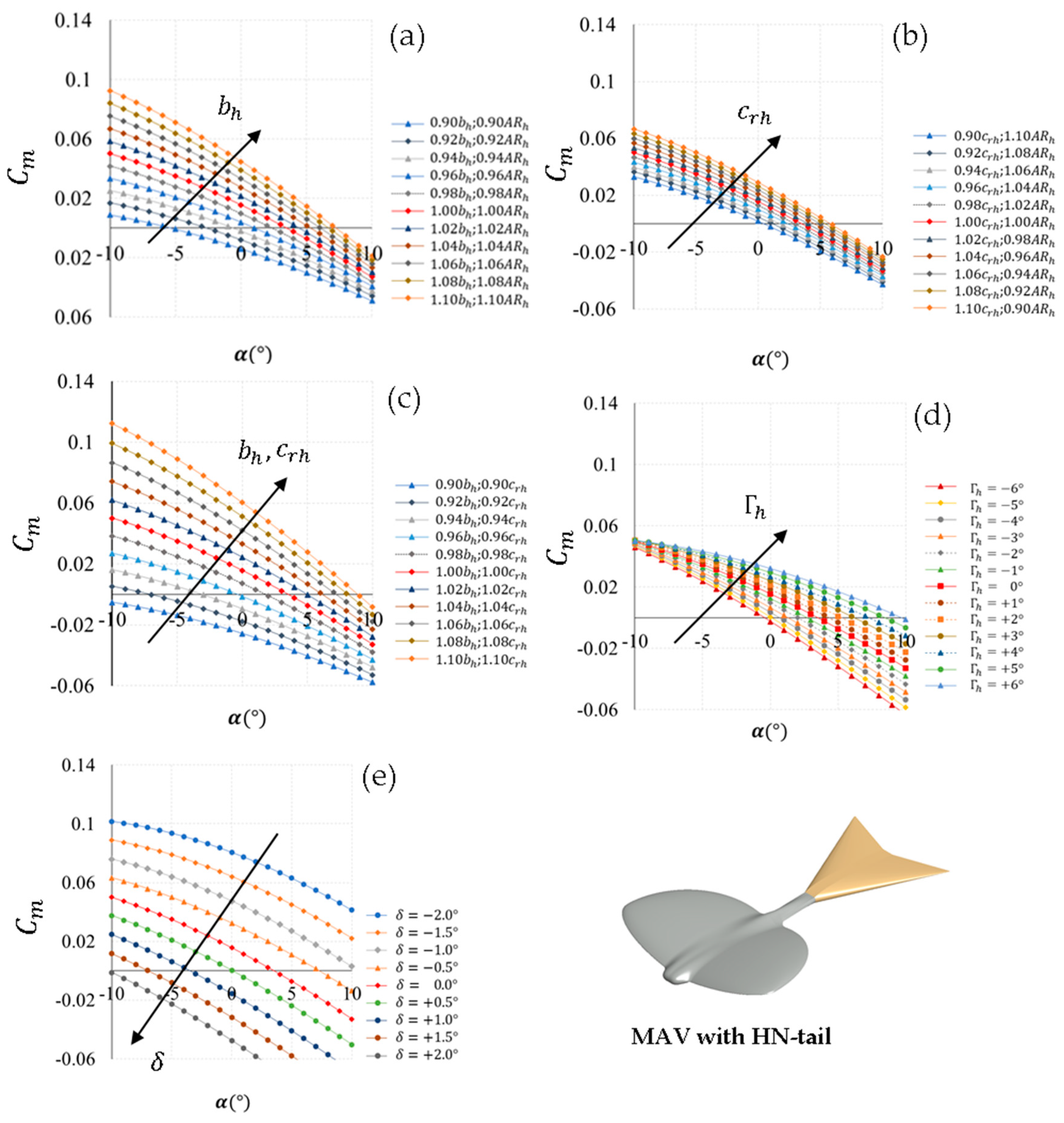
In this sub-section, numerical data obtained from the MAV vehicle with the HN-tail configuration are presented, due to that this tail produces the highest value of the maximum lift coefficient ($C_{Lmax}$). The remaining tail configurations present the same trend in lift coefficient and longitudinal stability, as the geometrical parameters of each tail configuration are varied ($b_h,c_{rh},{AR}_h,{\mathsf{\Gamma }}_h\mathrm{a}\mathrm{n}\mathrm{d}\delta$). The analysis of the results is valid for each of the tail configurations.

When the tail span ${(b}_h$) increases and the tail root chord ($c_{rh})$ remains constant, the longitudinal stability coefficient will be more negative, with an increase in the slope ($C_{m\alpha }$). Therefore, $C_{m0}$ increases as the tail span increases, so the curves move up along the vertical axis. 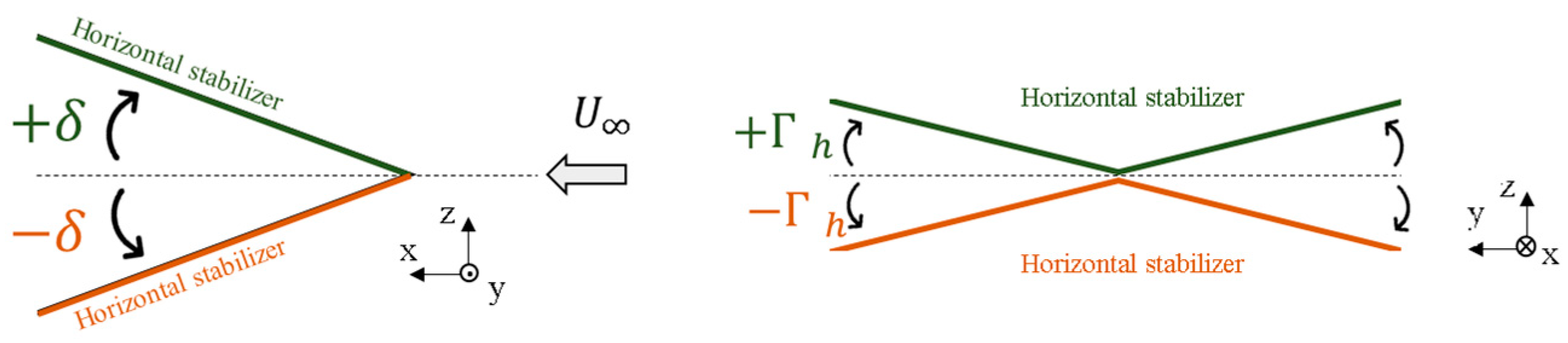The same behavior occurs in cases where the tail root chord $\left(c_{rh}\right)$ increases, when both the tail span ${(b}_h$) and root chord $c_{rh}$ increase, or when the dihedral angle increases (${\mathsf{\Gamma }}_h$). 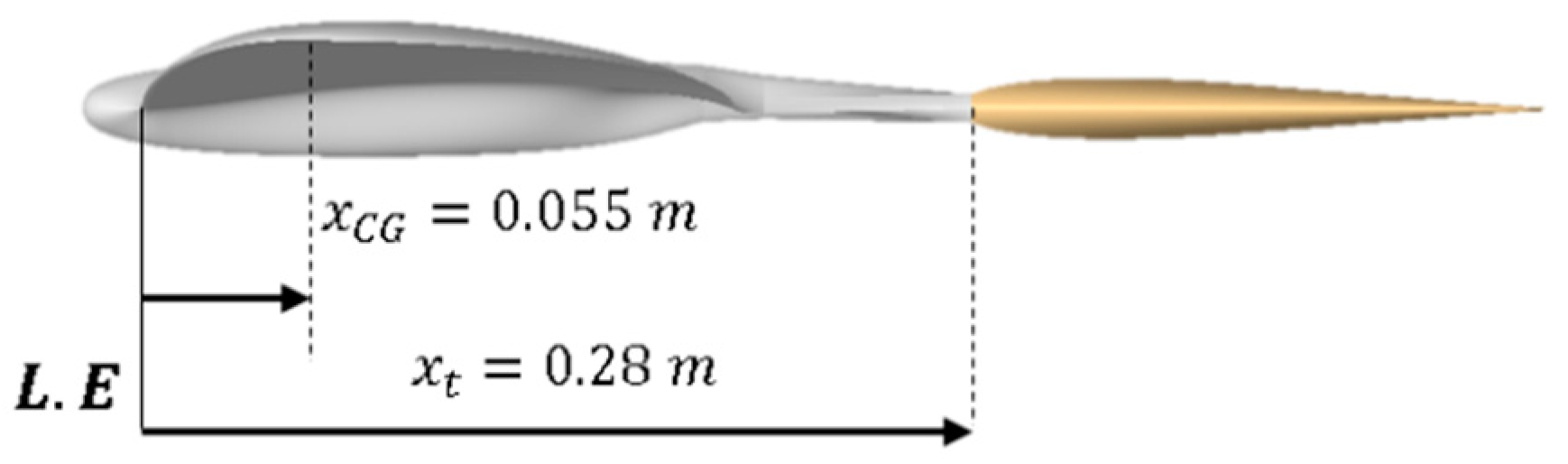As the angle of incidence of the horizontal stabilizer ($\delta$) increases, the longitudinal distance of the center of gravity $\left(x_{cg}\right)$ will increase, so the distance between the aerodynamic center $\left(CA\right)$ and the center of gravity $\left(CG\right)$ will decrease, and this causes the slope $C_{m\alpha }$ to become more positive (that is, less pronounced). Contrary to the previous cases, the value of $C_{m0}$ decreases as the incidence angle increases (curves are shifted downward) (see Figure 12).

6.2. Criteria for the Selection of the Optimal Tail Configurations

In this sub-section, two configurations of each type of the tail are selected (defined as C.1 and C.2 in

Table 7. Geometrical features of the optimal tail configurations.

Nomenclature	Tails	${\mathit{b}}_{\mathit{h}}\left(\mathbf{m}\mathbf{m}\right)$	${\mathit{c}}_{\mathit{r}\mathit{h}}\left(\mathbf{m}\mathbf{m}\right)$	${\mathbf{A}\mathbf{R}}_{\mathit{h}}$	${\mathsf{\Gamma }}_{\mathit{h}}(°)$	$\mathit{\delta }(°)$
$\mathrm{R}-\mathrm{H}\mathrm{W}-\mathrm{t}\mathrm{a}\mathrm{i}\mathrm{l}$		200	170	2.10	0	0
$\mathrm{C}.1-\mathrm{H}\mathrm{W}-\mathrm{t}\mathrm{a}\mathrm{i}\mathrm{l}$		196	170	2.05	−1	0
$\mathrm{C}.2-\mathrm{H}\mathrm{W}-\mathrm{t}\mathrm{a}\mathrm{i}\mathrm{l}$		200	173.4	2.05	−1	0
$\mathrm{R}-\mathrm{H}\mathrm{N}-\mathrm{t}\mathrm{a}\mathrm{i}\mathrm{l}$		200	170	2.10	0	0
$\mathrm{C}.1-\mathrm{H}\mathrm{N}-\mathrm{t}\mathrm{a}\mathrm{i}\mathrm{l}$		196	170	2.05	−1	0
$\mathrm{C}.2-\mathrm{H}\mathrm{N}-\mathrm{t}\mathrm{a}\mathrm{i}\mathrm{l}$		200	173.4	2.05	−1	0
$\mathrm{R}-\mathrm{H}\mathrm{S}\mathrm{F}-\mathrm{t}\mathrm{a}\mathrm{i}\mathrm{l}$		200	170	2.1	0	0
$\mathrm{C}.1-\mathrm{H}\mathrm{S}\mathrm{F}-\mathrm{t}\mathrm{a}\mathrm{i}\mathrm{l}$		200	170	2.1	3	0
$\mathrm{C}.2-\mathrm{H}\mathrm{S}\mathrm{F}-\mathrm{t}\mathrm{a}\mathrm{i}\mathrm{l}$		200	170	2.1	2	0
$\mathrm{R}-\mathrm{H}\mathrm{R}\mathrm{F}-\mathrm{t}\mathrm{a}\mathrm{i}\mathrm{l}$		200	170	2.1	0	0
$\mathrm{C}.1-\mathrm{H}\mathrm{R}\mathrm{F}-\mathrm{t}\mathrm{a}\mathrm{i}\mathrm{l}$		196	166.6	2.1	−1	0
$\mathrm{C}.2-\mathrm{H}\mathrm{R}\mathrm{F}-\mathrm{t}\mathrm{a}\mathrm{i}\mathrm{l}$		196	166.6	2.1	−2	0
$\mathrm{R}-\mathrm{H}\mathrm{F}\mathrm{K}-\mathrm{t}\mathrm{a}\mathrm{i}\mathrm{l}$		215	121	2.1	0	0
$\mathrm{C}.1-\mathrm{H}\mathrm{F}\mathrm{K}-\mathrm{t}\mathrm{a}\mathrm{i}\mathrm{l}$		215	121	2.1	3	0
$\mathrm{C}.2-\mathrm{H}\mathrm{F}\mathrm{K}-\mathrm{t}\mathrm{a}\mathrm{i}\mathrm{l}$		215	121	2.1	2	0

) to improve the longitudinal stability of the MAV. To achieve this, the minimum aerodynamic drag criterion $C_{Dmin}$ in the cruise phase was established. The angles of attack in the cruise phase where there is minimum drag are in the range of $0°\le \alpha \le 4°$. Therefore, the valid configurations will be all those in which the $C_m$ curve cuts with the axis within the established range of the angles of attack in the cruise phase (0°–4°) (see Figure 12). When there are more than two configurations in the valid angle of attack range (0°–4°), the next criterion to be taken into account is to select the greatest $C_m$, resulting in greater longitudinal stability. Thus, for each type of horizontal tail, two configurations with different geometrical parameters were selected. Table 7 shows the geometrical features of the two optimal tail configurations and the reference tail defined by −R.

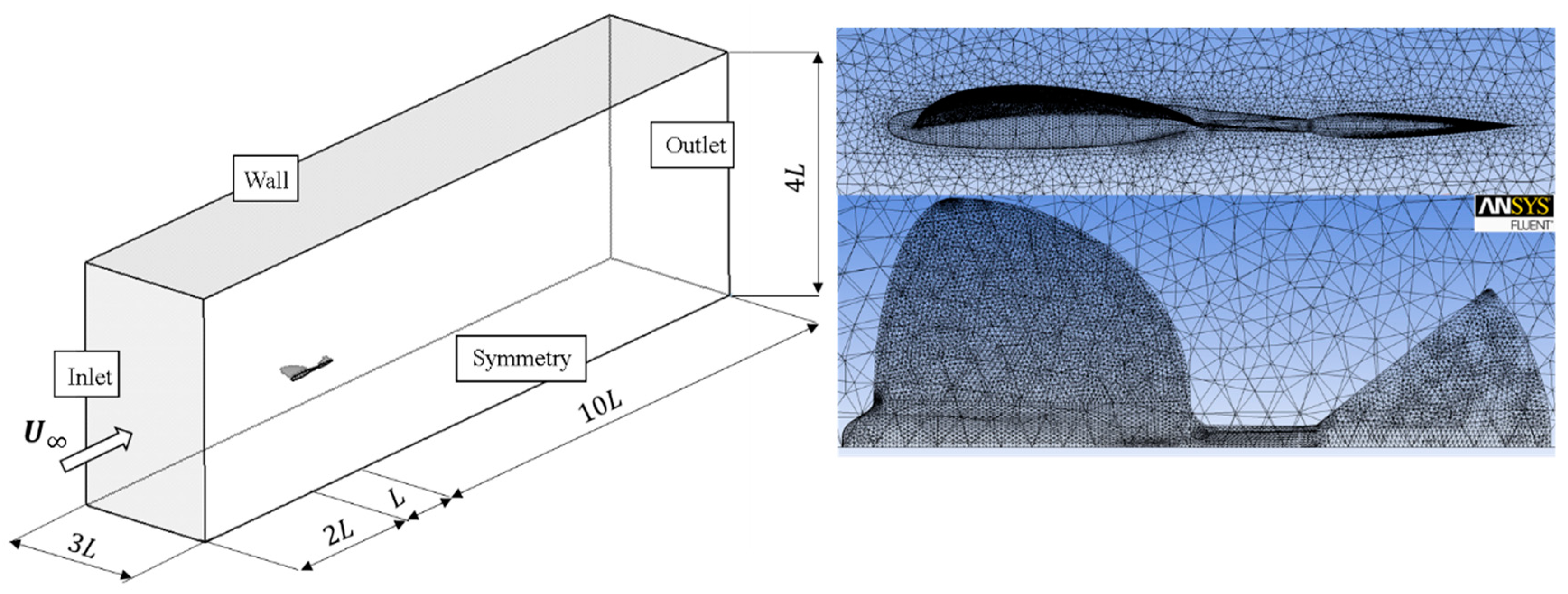
6.3. CFD Study

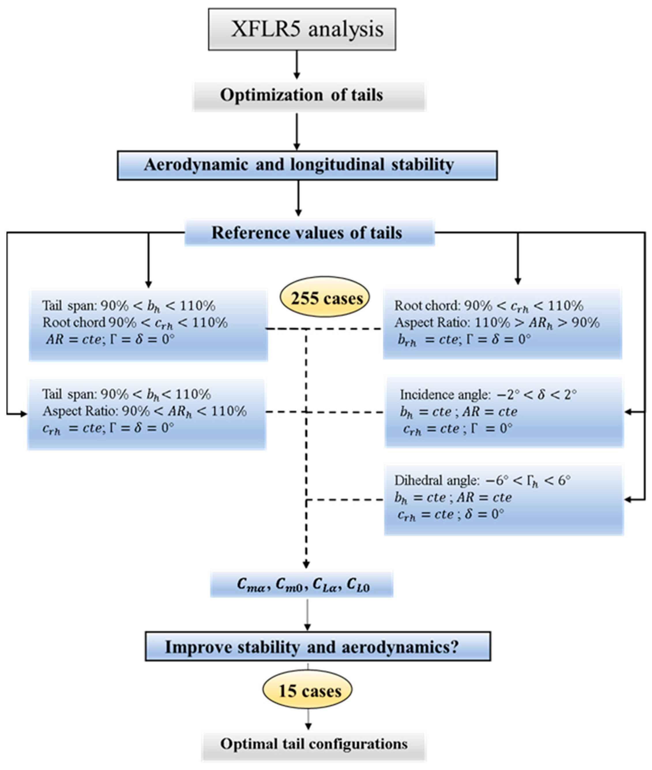
In this section, the numerical data obtained by CFD simulations for the 15 tail configurations defined in

Table 8. Variation in the aerodynamic parameters in HSF-tail.

	R-HSF-Tail	C.1-HSF-Tail	C.2-HSF-Tail
$C_{Lmax}$	1.89	$\uparrow 2.91\%$	$\uparrow 1.66\%$
$C_{Dmin}$	0.0635	$\downarrow 1.81\%$	$\downarrow 1.80\%$
$E_{max}$	6.63	$\downarrow 0.14\%$	$\downarrow 0.09\%$

are presented. Lift and drag coefficients, polar curve and aerodynamic efficiency for each of the tail configurations were obtained.

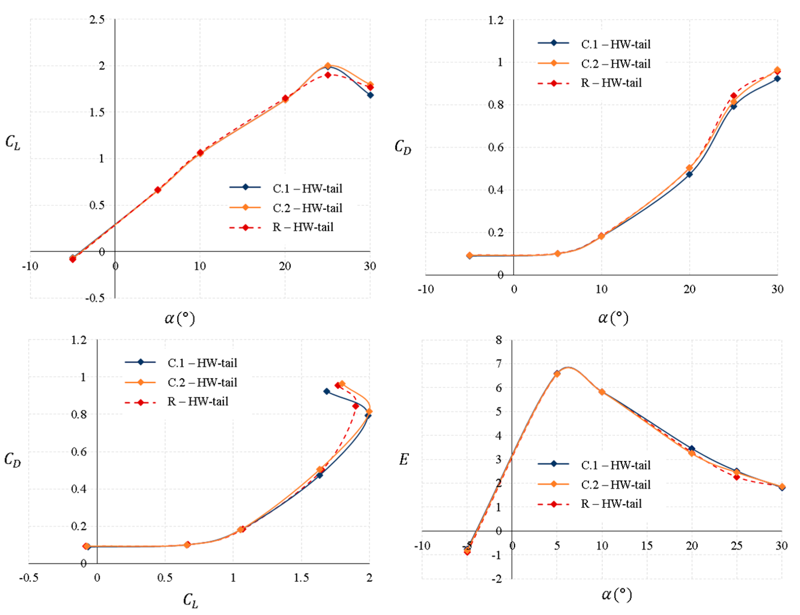
Figure 13 shows the aerodynamic characteristics of the MAV with the HW-tail. The lift coefficient values are very similar for all tail configurations at low angles of attack until reaching the angle of 25°. At this angle, the maximum lift coefficient is obtained for all tail configurations, being higher for the optimal tail configurations (C.1-HW-tail and C.2-HW-tail) than the reference tail configuration (R-HW-tail) due to the decrease in the dihedral angle and the variation in tail span and root chord. Although it is clear from these results that the maximum lift coefficient is obtained at 25°, the flow detachment could be between 20° and 25°, as the step is 5°. The drag coefficient and aerodynamic efficiency values are highly similar for all configurations until the angle of attack of 15°. However, for higher angles of attack, there is a decrease in drag of around 2.15% and an increase in aerodynamic efficiency of around 2.30% in the optimal tail configurations, due to that the dihedral angle is ${\mathsf{\Gamma }}_h=-1$ with slight variations in the tail span and chord.

Table 9. Variation in the aerodynamic parameters in HW-tail.

	R-HW-Tail	C.1-HW-Tail	C.2-HW-Tail
$C_{Lmax}$	1.76	$\uparrow 12.42\%$	$\uparrow 13.15\%$
$C_{Dmin}$	0.0632	$\downarrow 1.27\%$	$\downarrow 1.23\%$
$E_{max}$	6.58	$\uparrow 0.27\%$	$\downarrow 0.05\%$

shows the variations in the maximum lift coefficient ($C_{Lmax}$), minimum drag coefficient ($C_{Dmin}$) and maximum aerodynamic efficiency ($E_{max}$) for the HW-tail. Decreasing the tail span (C.1-HW-tail) or increasing the tail root chord (C.2-HW-tail) by 2% with respect to the reference values and with a negative dihedral angle has the same effect on the aerodynamic parameters. In both tail configurations, there is a slight decrease in the value of $C_{Dmin}$, a strong increase in $C_{Lmax}$ up to 13% and practically no change in aerodynamic efficiency. It seems that the decrease in the tail span (C.1-HW-tail) would give a slight improvement in the aerodynamic performance of the vehicle.

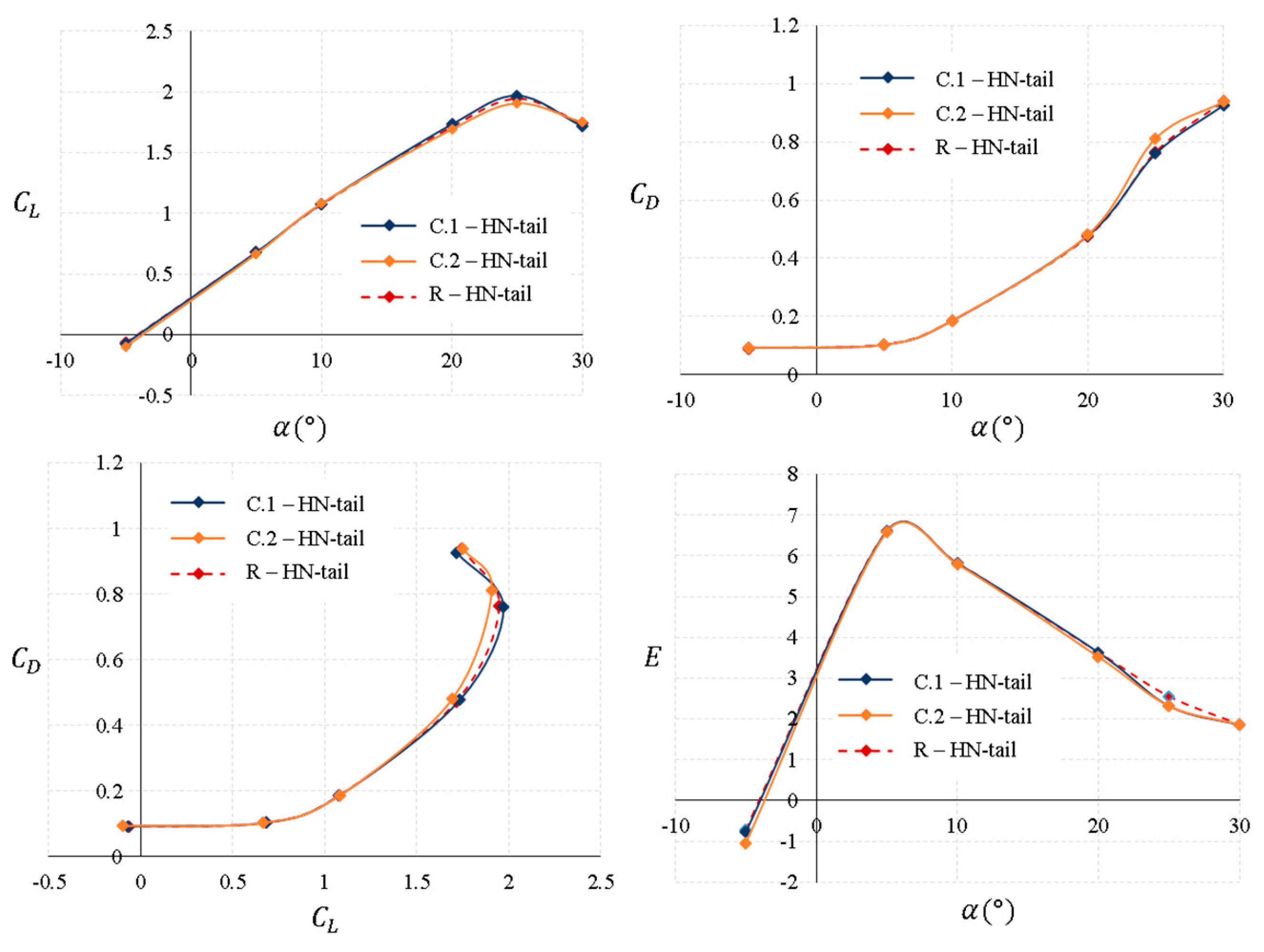
Figure 14 shows the aerodynamic characteristics of the MAV with the HN-tail. These tail parameters are the same as in the previous case. There is a decrease in the tail span of 2% for the C.1-HN-tail and an increase in the root chord of 2% for the C.2-HN-tail, with the same negative dihedral angle in both of them. In this tail configuration, it is clearly observed from the graphs that the variations in the geometrical parameters are much less noticeable than in the previous tail configuration (HW-tail). During all ranges of the angles of attack, the values of lift, drag and aerodynamic efficiency are not greatly affected by the variation in the geometrical parameters.

Table 10. Variation in the aerodynamic parameters in HN-tail.

	R-HN-Tail	C.1-HN-Tail	C.2-HN-Tail
$C_{Lmax}$	1.94	$\uparrow 1.09\%$	$\downarrow 2.13\%$
$C_{Dmin}$	0.0645	$\downarrow 0.09\%$	$\downarrow 0.08\%$
$E_{max}$	6.59	$\uparrow 0.16\%$	$\downarrow 0.11\%$

shows a summary of the aerodynamic parameter variation between all HN-tail configurations. In both tails, there is practically no change in $E_{max}$ and $C_{Dmin}$ with respect to the reference tail. However, $C_{Lmax}$ is deteriorated by around 2% when the tail root chord increases from the reference values. Taking into account these data, the tail span reduction could be the one that generates less drag, with a small improvement on the overall performance of the MAV.

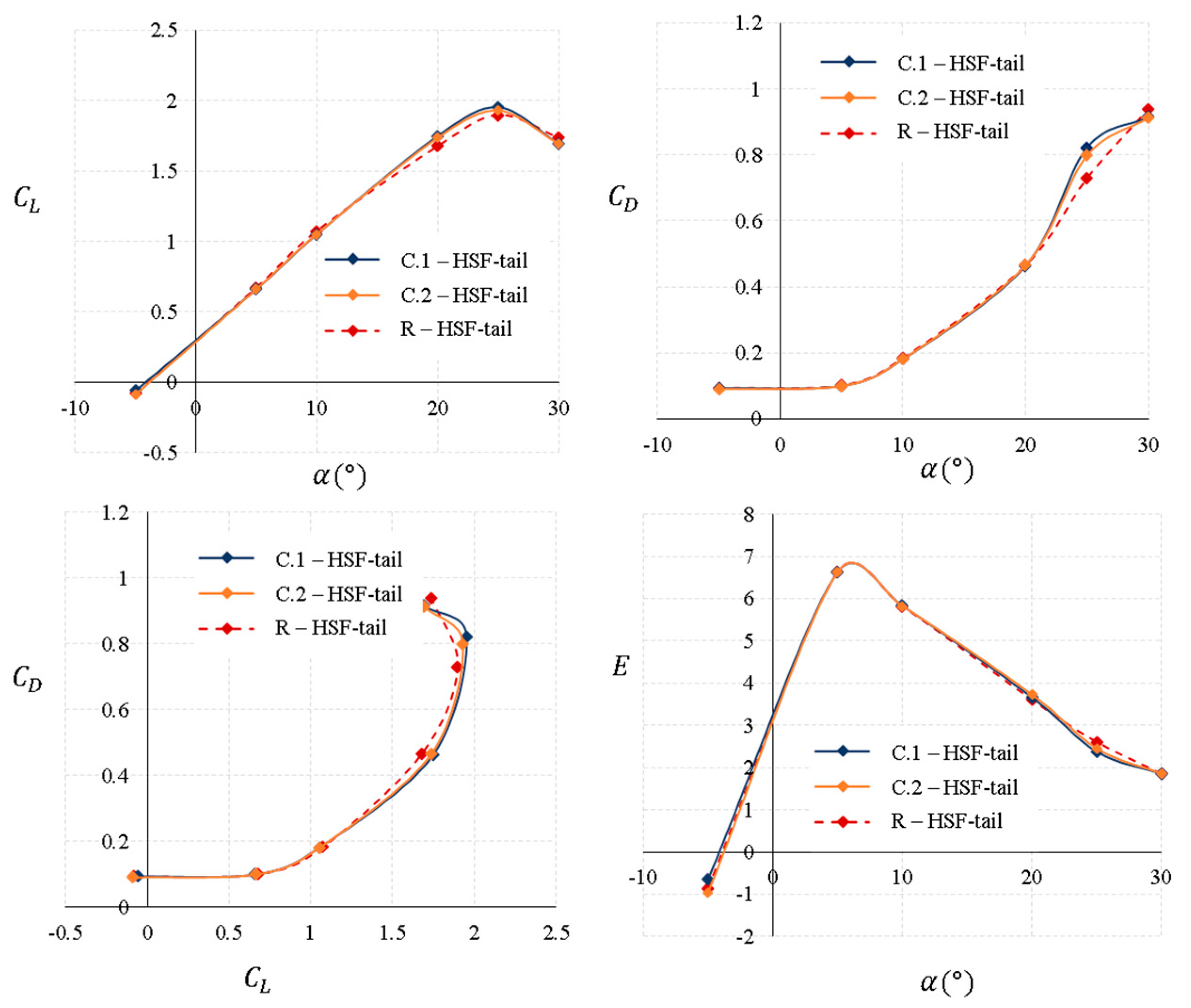
Figure 15 shows the aerodynamic characteristics of the MAV with the HSF-tail. In this tail configuration, only the dihedral angle is varied, being ${\mathsf{\Gamma }}_h=3°$ for the C.1-HSF-tail and ${\mathsf{\Gamma }}_h=2°$ for the C.2-HSF-tail. When the dihedral angle increases, there is an increase in the $C_{Lmax}$, being higher for ${\mathsf{\Gamma }}_h=3°$, and also there is a decrease in the value of the minimum aerodynamic drag coefficient of up to 1.80% for both tail configurations. The variations in the aerodynamic parameters in this tail configuration are minimal between all of them. The maximum aerodynamic efficiency is practically the same for all tails. It could be concluded that the one that provides a slight increase in the performance of the vehicle will be the C.1-HSF-tail with a dihedral angle of ${\mathsf{\Gamma }}_h=3°$.

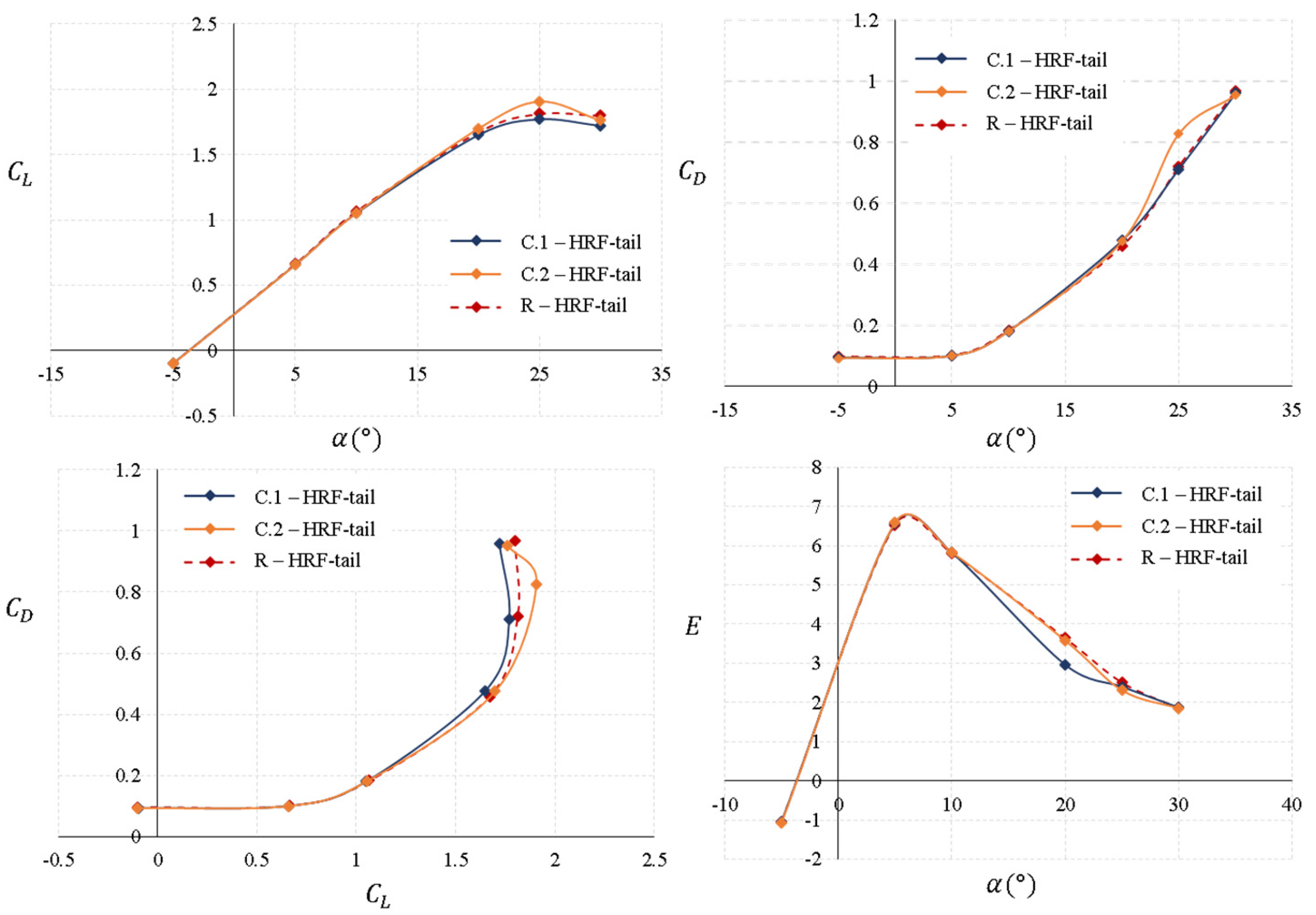
Figure 16 shows the aerodynamic characteristics of the MAV with the HRF-tail. In this case, the two tail configurations show a decrease in the tail span and chord of 2% compared to the reference dimensions, but with a dihedral angle for the C.1-HRF-tail of ${\mathsf{\Gamma }}_h=-1$ and for the C.2-HRF-tail of ${\mathsf{\Gamma }}_h=-2$. Lift, drag and aerodynamic efficiency values are very similar for all tail configurations for angles of attack below 20°.

In

Table 11. Variation in the aerodynamic parameters in HRF-tail.

	R-HRF-Tail	C.1-HRF-Tail	C.2-HRF-Tail
$C_{Lmax}$	$1.81$	$\downarrow 2.40\%$	$\uparrow 5.11\%$
$C_{Dmin}$	$0.0639$	$\downarrow 1.49\%$	$\downarrow 1.72\%$
$E_{max}$	$6.53$	$\uparrow 0.60\%$	$\uparrow 0.82\%$

, a summary of the aerodynamic characteristics is presented for the HRF-tail. The greatest value for the maximum lift coefficient is obtained for the C.2-HRF-tail configuration, with the most negative dihedral angle being up to 5.11% higher than for the reference tail configuration. From the data in the table, it is observed that a decrease in the span and root chord and negative dihedral angles give lower values of drag during cruise flight, being the lowest value for the C.2-HRF-tail configuration. In both optimal tail configurations, there is no notable variation in the aerodynamic efficiency. To conclude, the tail configuration that will provide the highest performance to the MAV will be the configuration with 2% less tail span and tail chord and a dihedral angle of ${\mathsf{\Gamma }}_h=-2$ (C.2-HRF-tail).

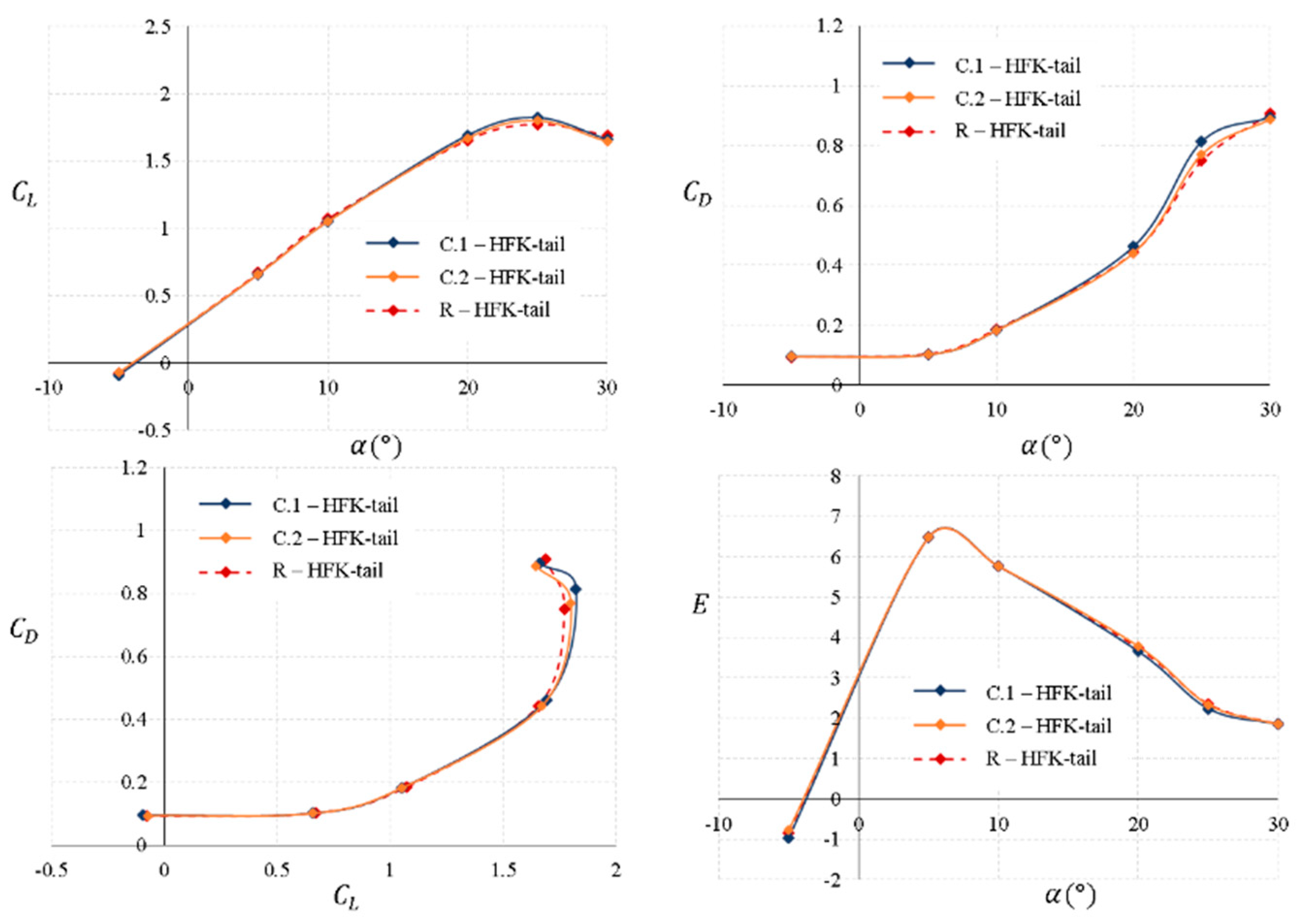
Figure 17 shows the aerodynamic characteristics of the MAV with the HFK-tail. In this case, the tail geometrical parameters vary as in the case of the HSF-tail configuration. Only the dihedral angle is varied, being ${\mathsf{\Gamma }}_h=3°$ for the C.1-HFK-tail and ${\mathsf{\Gamma }}_h=2°$ for the C.2-HFK-tail, while the tail span and chord maintain the same value as in the reference tail configuration. Lift, drag and aerodynamic efficiency values are very similar for all tail configurations until the angle of attack of 20° is reached. By increasing the dihedral angle, the maximum lift coefficient can reach a value slightly above than the reference tail configuration at the angle of 25°.

Table 12. Variation of the aerodynamic parameters in HFK-tail.

	R-HFK-Tail	C.1-HFK-Tail	C.2-HFK-Tail
$C_{Lmax}$	$1.77$	$\uparrow 2.87\%$	$\uparrow 1.58\%$
$C_{Dmin}$	$0.0647$	$\downarrow 1.54\%$	$\downarrow 1.53\%$
$E_{max}$	$6.47$	$\uparrow 0.015\%$	$\downarrow 0.07\%$

summarizes the variation in the aerodynamic parameters of $C_{Lmax}$, $C_{Dmin}$ and $E_{max}$ for the HFK-tail. The value of the minimum drag coefficient can be reduced by around 1.54% of that of the reference tail by increasing the dihedral angle. The increase in the dihedral angle leads to a slight increase in $C_{Lmax}$, being more notable for the case of ${\mathsf{\Gamma }}_h=3°$ (C.1-HFK-tail). However, there are no appreciable changes in the maximum aerodynamic efficiency. The tail configuration that could provide a slight improvement in the aerodynamic characteristics would be the configuration of ${\mathsf{\Gamma }}_h=3°$ (C.1-HFK-tail).

After analyzing all the tail configurations, a final selection was made based on the criterion of maximum aerodynamic efficiency ($E_{max}$) in the cruise phase. Therefore, only one configuration of each tail type was chosen as a possible solution to be implemented in the vehicle.

Table 13. Final selection of the tail configurations.

	C.1-HW	C.1-HN	R-HSF	C.1-HRF	C.1-HFK
$C_{Dmin}$	0.0624	0.0644	0.0635	0.0629	0.0637
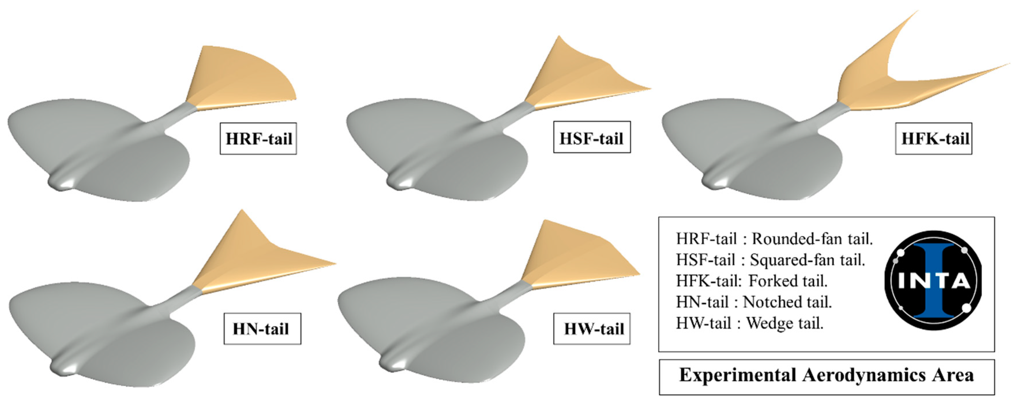
$E_{max}$	6.59	6.60	6.63	6.57	6.47

shows the five selected tail configurations (with the tail geometrical parameters defined in Table 8). The squared-fan tail (HSF-tail) provides the highest aerodynamic efficiency value, $E_{max}$ = 6.63, followed by the notched-tail (HN-tail), wedge-tail (HW-tail), rounded-fan tail (HRF-tail), and in the last position, the forked-tail (HFK-tail), with around 2.50% less aerodynamic efficiency.

According to these results, the selected tail configuration to improve the aerodynamic efficiency and increase the longitudinal stability of the vehicle would be the squared-fan tail (HSF-tail).

7. Conclusions

Inspiration from nature to develop new MAV designs has been of great interest for many years. In this paper, a numerical analysis of horizontal stabilizers inspired by the most general bird tails (rounded, fan-shape, squared, forked, notched and wedge tails) for the implementation in the MAV developed between INTA and UPM is presented. The study is mainly focused on improving the longitudinal stability and aerodynamics of this vehicle through bioinspiration.

In a first step, a preliminary optimization of the five proposed bird tails was performed using XFLR5 by varying several geometrical parameters of the tail in order to obtain the longitudinal stability of the MAV. A total of 255 cases were simulated. The sensitivity analysis of the tail geometric parameters to check the longitudinal stability of the vehicle shows that an increase in the tail span ($b_h$), chord $c_h$ or dihedral angle (${\mathsf{\Gamma }}_h$) will directly improve longitudinal stability. On the contrary, an increase in the angle of incidence ($\delta$) of the tail will decrease the longitudinal stability. Then, the aerodynamic analysis with CFD was performed only for the longitudinal stable cases of each tail type that met the established requirements of minimum aerodynamic drag in the cruise phase. A total of 15 CFD cases (three configurations per tail) were performed. From all these, only one configuration of each tail was finally obtained as a possible solution to be implemented in the MAV. The last comparison of the results shows that the squared-fan tail (HSF-tail) has the greatest performance in terms of maximum aerodynamic efficiency, $\frac{C_L}{C_D}$, while maintaining the high longitudinal stability of the vehicle during cruise flight. Consequently, this HSF configuration of the horizontal stabilizer inspired by bird tails should be implemented in the future real demonstration of this MAV.

To conclude, this paper provides an innovative study in the developing MAV field due to the implementation of a bioinspired horizontal stabilizer for improving longitudinal stability and aerodynamic performance in an MAV with Zimmerman wing-body geometry.