Abstract
We introduce algorithmic advancements designed to expedite simulations in OpenFOAM using GPUs. These developments include the following. (a) The amgx4Foam library, which connects the open-source AmgX library from NVIDIA to OpenFOAM. Matrix generation, involving tasks such numerical integration and assembly, is performed on CPUs. Subsequently, the assembled matrix is processed on the CPU. This approach accelerates the computationally intensive linear solver phase of simulations on GPUs. (b) Enhancements to code performance in reactive flow simulations, by relocating the solution of finite-rate chemistry to GPUs, which serve as co-processors. We present code verification and validation along with performance metrics targeting two distinct application sets, namely, aerodynamics calculations and supersonic combustion with finite-rate chemistry.
1. Introduction
Computational Fluid Dynamics (CFD) has become a mature technology in engineering, where it contributes strongly to industrial competitiveness and sustainability across a wide range of sectors [1,2]. On the other hand, the current and future growth of CFD depends upon the exploitation of massively parallel High-Performance Computing (HPC) hardware technology, which in recent years has seen a significant evolution towards the exascale. One example is Graphical Processing Units (GPUs). GPUs are best suited for numerical applications that prioritize high throughput and involve processing large quantities of independent datasets [3]. A GPU can work together with a Central Processing Unit (CPU) to accelerate scientific, analytic, engineering, and enterprise applications. There is a fundamental difference in architectural design between a GPU and CPU. GPUs are basically many-core processors having thousands of cores designed to deliver high computational throughput, whereas CPUs sacrifice the computational throughput of the processor to increase the performance of a single core. This different design philosophy necessitates the development of specialized algorithms to exploit the potential performance of GPU hardware. The implementation of GPU porting in CFD is interesting due to its capacity to enhance performance, decrease computational time, manage substantial datasets, streamline multiphysics simulations, support optimization and design exploration efforts, and contribute to scientific progress by enabling simulations of heightened complexity and precision. The main benefits of using GPUs for CFD simulations are currently justified by their reduced hardware cost and limited power consumption. HPC and GPU computing is expected to have a significant impact on multiphysics CFD [4,5,6,7]. In multiphysics CFD simulations, multiple governing equations representing different physics, such as fluid flow, heat transfer, fluid–spray particle interaction, chemical reactions, and solid mechanics can be solved. These equations may have different nonlinearities and couplings that make it difficult to solve them as a single system of equations. In CFD solvers, operator splitting [8] is a way to break down complex problems into simpler subproblems, possibly with different timescales that can be solved sequentially as separate sets of equations. Such computations are very common in aeronautics and aerospace, where the solution of fluid transport is coupled to Lagrangian Particle Tracking in spray simulations, the deformation of solids in aeroelastic calculations, or the solution of finite-rate chemistry problems in reactive flow/combustion simulations. The main feature of operator splitting is that it allows for the use of different numerical methods and algebra solvers optimized for each specific subproblem; this has traditionally been done to achieve improved overall stability and efficiency of the solution. Operator splitting can facilitate optimization of the CFD software for exascale hardware. Developers can fine tune and adapt different solvers for each subproblem to take full advantage of the available computational power, memory bandwidth, and interconnections in exascale systems [9,10]. The study of methods to accelerate computation is a traditional subject in Computational Fluid Dynamics (CFD). Many research papers and articles have been published exploring the acceleration of various CFD solvers using GPUs [7,11,12,13,14,15,16,17,18,19,20,21,22,23,24,25,26,27,28,29]. These papers often discuss implementing parallelization strategies, porting solvers to GPU architectures, and optimizing computation to take advantage of GPU capabilities.
1.1. Motivation of This Work
The primary goal of this research is to introduce advanced algorithmic enhancements targeted at accelerating Computational Fluid Dynamics (CFD) computation in the aerospace domain by utilizing Graphics Processing Units (GPUs) within the OpenFOAM framework. The focus is centered on porting algebraic solvers for both Partial Differential Equations (PDEs) and Ordinary Differential Equations (ODEs) on GPUs. These solvers are the fundamental elements of multiphysics CFD software enabling numerical simulation of complex fluid flow phenomena. The extent of acceleration provided by the GPU varies based on the specific problem, necessitating progressive software development, collaborative redesign, and crucially, enhancements in solver technology algorithms to facilitate targeted simulation capabilities.
Because this is a fairly new area there is only a limited body of literature addressing multiphysics CFD simulations and the porting of these simulations to GPUs. Specifically, there has not been very much discussion about which improvements in algorithms can be helpful for solving practical multiphysics CFD problems. To the best of our knowledge, there are no examples in which fast GPU simulations have been demonstrated for complex multiphysics CFD problems that are important in real world applications within the OpenFOAM framework. Thus, we explore these aspects in this paper.
1.2. Highlights
This paper elaborates on the theoretical foundations of evolutionary advancements made by the authors in the open-source CFD software OpenFOAM aimed at achieving exascale capabilities through the utilization of GPU potential. To achieve this goal, two key strategies are employed: (a) the acceleration of iterative sparse linear system solutions through the implementation of the external module amgx4foam, linking OpenFOAM to the NVIDIA AmgX library [21,30]; and (b) the vectorization/hybridization of GPGPU reactive flow solvers, which involves the migration of compute-intensive operations to GPUs which function as co-processors. The verification of these software components is conducted on benchmark test cases where reference solutions are available. Furthermore, assessment is carried out on impactful applications within the automotive and aerospace domains, namely, accelerating the solution of aerodynamics for external flows and enhancing the speed of combustion simulations.
Algorithmic advancements are realized in the form of an external library module that is dynamically linked to the latest releases of OpenFOAM [31,32]. This module serves to accelerate all types of solvers present in the legacy code, spanning compressible, incompressible, and reacting multiphase scenarios.
1.3. Paper Structure
This paper’s structure is outlined as follows. Initially, we describe the operator splitting technique used in Finite Volume (FV) Computational Fluid Dynamics (CFD) solvers in Section 2. This provides insight into the architecture of the CFD code and underscores the close relationship between software architecture, GPU porting strategies, and the underlying numerical methods. Section 3 is dedicated to the adaptation of algebraic solvers for the Partial Differential Equations (PDEs) governing fluid transport to GPU platforms. We present performance metrics obtained from a benchmark case involving external aerodynamics calculations in which the solution of the linear algebra problem is offloaded to the NVIDIA AmgX library. In Section 4, we shift our focus to accelerating Ordinary Differential Equations (ODEs), which are commonly used in submodels for multiphysics CFD simulations. This section explores the intricate interplay between flow transport, species transport, and finite-rate chemistry, discussed in detail in Section 4.1, and the rationale behind the implementation of a fast GPGPU solver in FV CFD solvers, discussed in Section 4.2 and Section 4.3. We then present the validation and verification results for the implemented methodologies in Section 4.4. In Section 4.6, we apply and validate these techniques to simulate supersonic combustion in a scramjet engine. Performance metrics for reactive flow simulations are provided in Section 4.8. The conclusions of our study are summarized in Section 5.
2. Implicit Segregated Solution Method of the Flow Transport for All Flow Speeds
In a CFD solver, the sequential solution of the governing equations for the flow transport in a Eulerian frame of reference reads
where , , p, and T are the fluid density, velocity, pressure, and temperature, respectively; is the viscous part of the stress tensor; is the total energy density, with e being the specific internal energy; the diffusive heat flux is defined as positive for cooling, where is the thermal conductivity of the flow; the terms and are the sources and sinks for momentum and energy, respectively; and is the heat released by chemical reactions, if present. The flow transport problem (Equations (1)–(3)) is solved by a SIMPLE-type pressure-based compressible unsteady segregated flow solver [33] for unstructured polyhedral grids for all flow speeds [8]. The linearized equations for the velocity components, species transport, energy, and pressure correction are solved in turn until the coupling of the primary variables is reached. As all terms are discretized by a fully implicit scheme, nonlinear terms (fluxes and source terms) are linearized and computed at the new time level and the equations are solved iteratively. In the fully implicit unsteady solver, outer iterations (denoted as m in the following) are repeated multiple times while solving across the time interval [n; n + 1]; the outer loop ends when the entire set of nonlinear equations satisfies the solver’s stopping criteria. These iterations are different from the inner ones, which are performed on linear systems with fixed coefficients. Similar to the procedure employed by SIMPLE-type methods for incompressible flows [33], the momentum equations (where the pressure gradient can be neglected) are used to calculate an intermediate velocity field :
In Equation (4), the density comes from the previous outer iteration . If the flow viscosity depends on the temperature or other variables, the viscous terms are computed using quantities from the previous iteration. The velocity field obtained via the linearized momentum equations structured on the old pressure and density values does not satisfy the mass conservation equation. In fact, when the mass fluxes computed using these velocities and the old density are inserted into the continuity equation, a mass imbalance is produced in the volume V and must be eliminated by a correction method:
where
The second-order term in Equation (6) is assumed to go to zero more rapidly than the other terms, and as such is neglected. This approximation does not have any influence on the convergence rate or impact on the final solution, as it tends to zero at convergence. It follows that
in which is the surface normal vector and and are defined from
while
While the pressure gradient only corrects the flow velocity in low-Mach implementations, in pressure-based compressible solvers the pressure correction acts on the density. The first term of Equation (7) is similar to the term for incompressible flows, while the second term includes a density correction that goes to zero in cases with a low Mach number.
The intermediate velocity field calculated from the predictor step (Equation (4)) must be corrected by a pressure gradient to enforce mass conservation in the domain. The combination of Equations (5) and (6) written in differential form reads
Equation (11) is called the pressure correction equation; its solution determines the correction to be applied to the mass fluxes computed via the use of the intermediate velocity field . As the correction is carried out using the pressure, the thermodynamic state depends on the correction procedure as well. The time derivative in Equation (11) can be decomposed as follows:
In Equation (12), is the fluid compressibility (see Appendix A), while the coefficient depends on the adopted time differencing scheme. For the three-time-level scheme (backward Euler method) , while for the two-level first order implicit method 1. In addition (see Appendix A and Appendix B, respectively), we have
and
with the final form of the pressure correction equation written as follows:
Equation (15) includes an incompressible divergence term to correct the mass fluxes and a compressible convective term to correct the density. They alternatively become dominant when the flow is largely incompressible or compressible, respectively, making the pressure-correction strategy applicable over a wide range of applications at all flow speeds [8]. At low Mach number values, the correction term dominates and Equation (15) assumes an elliptic form for incompressible flow cases, while at high Mach numbers the contribution of the term containing is enlarged and Equation (15) assumes a hyperbolic form. Upon solving the pressure-correction equation, velocity and density are updated to obtain and ; these values are used to solve the energy equation at the next step, from which the updated internal energy is obtained. In turn, the temperature is determined via thermodynamics. The new density is computed from the EoS (see Appendix A):
and the velocity is updated
To achieve closure of the system, constitutive relations are needed. Their formulation depends on the properties of the continuous medium. The following set of constitutive relations is used:
- -
- The generalized form of the Newton’s law of viscosity:in which is the dynamic viscosity and is the identity matrix.
- -
- A nine-coefficient polynomial computes the thermodynamic properties in the standard state for each gaseous specie, as in the NASA chemical equilibrium code [34], to define the internal energy as a function of the pressure and temperature.
- -
- The Equation of State (EoS) for the gas, which is assumed to be mixture of species:where W is the mean molecular weight of the mixture. All the species of the mixture are treated as perfect gases with a common temperature T; each species is described by Mendeleev–Clapeyron EoS , with = 8.314 J/(mol K) being the perfect gas constant and and the partial pressure and density of the i-th species, respectively, with (Dalton law). Despite the assumption of a mixture of perfect gases being applied in this work, the solver natively supports real gas formulations as well.
- -
- Eddy–viscosity based models for turbulence closure.
3. Solution of Large Sparse Linear Systems in Segregated Solvers
In a segregated solver, these systems are constructed as part of the nonlinear process for a number of steps that varies with the specific algorithm (steady, unsteady) used to solve the governing equations. While all of the algorithms solve the same governing equations, they differ in how they loop over the equations. At every iteration, either the coefficient matrix changes or does not, while the right-hand side and the solution change from one step to the next. In Figure 1, the Semi-Implicit Method for Pressure Linked Equations (SIMPLE) and the Pressure Implicit with Splitting of Operator (PISO) are shown. These represent the most common algorithms in the FVM for steady and unsteady incompressible flow calculations respectively.
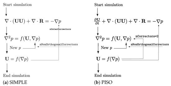
Figure 1.
Segregated solution of the fluid transport for incompressible flows in the Finite Volume Method for steady and unsteady problems: (a) Semi-Implicit Method for Pressure-Linked Equations (SIMPLE) and (b) Pressure Implicit with Splitting of Operator (PISO). Each equation implies the solving of a large sparse linear system.
In both the algorithms, the incompressibility constraint is used to bypass fast acoustic waves and allow the solution to evolve on a convective timescale, which is relevant for many engineering problems. This leads to a very stiff Poisson problem; thus, the pressure solver typically encompasses the majority of the solution time (over 60% of the time for a single step of computation in the SIMPLE algorithm [9,21]). The computation of the predictor step is usually not very expensive, and the speed-up provided by the GPU is negligible.
Behind any solution method for the fluid transport in the Finite Volume method lies the solution of large sparse linear systems, which we write as
where the coefficient square sparse matrix A is , while and b. The sparsity graph of the square matrix generated through the discretization of an advection–diffusion-reaction problem using Finite Volume exhibits two main properties: (a) the diagonal elements consistently align with non-null elements and (b) the sparsity pattern displays symmetry. In OpenFOAM, a square matrix is represented as a data structure that stores its values along with a pointer to its associated sparsity pattern, which is depicted using two integer vectors. The length of such vectors is equal to the number of faces, and indicates the labels of the owner and the neighboring cell, respectively. Saving the sparsity pattern prevents redundant storage of identical pattern structures when multiple matrices share the same sparse pattern. The combination of the three mentioned vectors defines the Co-Ordinate List format (COO), which is usually an ordered list. For a nonsymmetric square matrix, the LDU factorization is A = LDU, where L is a unit lower triangular matrix, U is an upper triangular matrix, and D is a diagonal matrix. The diagonal matrix is stored compactly as a vector, and its pattern is implied. Because the sparsity pattern of the upper triangular matrix (U) is the same as the lower triangular matrix (L), saving the pattern of either matrix is sufficient. For symmetric matrices, only the values of U require storage. The Compressed Sparse Row (CSR) format is another general compressed sparse matrix format supported by High Performance Computing (HPC) libraries [35,36,37,38] for scientific and computational applications, and can help to save memory and improve computational efficiency in operations involving large sparse matrices. It is in fact possible to completely access the matrix elements by saving only the indices of the start of a new line, reducing the total number of indices needed to represent a matrix from M to N. This reduction in the number of indices translates directly to a reduction of the amount of data needing to be transferred from the main memory to the processors for Sparse Matrix Vector Multiplication (SpMVM) operations. The NVIDIA AmgX library [30] includes a collection of methods employing various selector and interpolation strategies. It incorporates many standard preconditioned Krylov subspace iterative methods [39,40,41], offering a range of smoothers and preconditioners. The work presented in this section builds on the foundation laid out in [21]. A wrapper is developed for AmgX to offload the linear solver tasks onto distributed NVIDIA GPUs. Because AmgX works with CSR matrices, the conversion of the OpenFOAM LDU matrix format into CSR form [42] has been refactored and seamlessly integrated into the dynamic library amgx4Foam, designed to be compatible with any OpenFOAM solver. The library’s architecture is designed for enhanced ease of use, installation, and maintenance while ensuring compatibility with both current and future software releases. The current approach carries out matrix assembly on the CPUs. This implies that there must be a balance between the number of available GPU cards and CPU cores. Having a large number of GPUs with only a small number of CPUs would not yield significant performance improvements, as data input/output and matrix assembly could become bottlenecks in the computations. Hence, for the calculations presented in this section (acceleration of flow tranport calculations), the optimal hardware configuration assumes one GPU per CPU node. This principle does not hold true in scenarios involving solving ordinary differential equations (ODEs) within reacting flow computations. In such cases, as the number of GPU cards increases, the capacity to simultaneously solve a larger number of systems of ODEs (up to the mesh size) grows as well. This contradicts the previously mentioned balance between GPU cards and CPU cores. In this context, having more GPUs in the same cluster node can enhance the capacity to handle multiple systems of ODEs simultaneously, potentially leading to improved performance. However, in scenarios where matrix assembly remains a computational bottleneck, the relationship between GPU cards and CPU cores as discussed earlier continues to hold. It is worth clarifying that the code implementation remains unaffected by the hardware configuration, and is capable of accommodating any number of CPU cores and GPU cards per node. Offloading the linear algebra solution to the GPU involved several additional steps, including converting the matrix format from LDU to CSR and transferring data between RAM and GPU memory. These processes introduce time overheads; thus, the overall computational efficiency of the GPU needs to consider the net performance gain. It is reasonable to anticipate that larger problem sizes would realize greater speedup benefits from GPU utilization.
The resulting implementation has undergone testing to accelerate the solution of steady aerodynamics for external flows. Performance testing was conducted on a cluster node featuring an Intel Xeon Gold 6248 CPU (2.50 GHz) and an NVIDIA Tesla V100. The tests were performed on a steady-state incompressible single-phase multi-dimensional Finite Volume solver (simpleFoam). The k-omega Shear Stress Transport (SST) model was employed as the turbulence model. The calculations for the momentum predictor and turbulence transport had minimal impact on the computations [8]. Thus, the GPU offloading was exclusively applied to the solution of the pressure (Poisson) equation. All computations were carried out in double precision. The Algebraic Multi-Grid (AMG) solver supported by AmgX [21] was employed as a preconditioner for various iterative Krylov outer solvers.
Performance comparisons were conducted as follows: CFD simulations were executed in OpenFOAM on the motorbike tutorial test case using different grid sizes (S, M, L). These simulations were run on 8, 16, and 32 CPU cores. Two solver configurations were compared: (a) Conjugate Gradient (CG) with simplified Diagonal-based Incomplete Cholesky (DIC) preconditioning and (b) Geometric Algebraic Multi-Grid (GAMG).
The predicted drag and lift forces are in strong agreement, confirming that the numerical setups used on the different technologies were consistent. This is apparent from the visual representations in Figure 2 and Figure 3 as well, which depict nearly identical pressure and velocity distributions around the motorbike for both the GPU and CPU methods. In addition, the differences in the predicted values of and are negligible (within 0.1%), validating the consistency of the numerical setups across various technologies, see Table 1. It is worth noting, however, that the implementation of implicit linear solvers within separate library codes varied for the GPU and CPU, as did the definition of the stopping criteria. While the fundamental theory governing the linear algebra solvers remains consistent, a direct one-to-one correspondence between OpenFOAM and AmgX is not present.
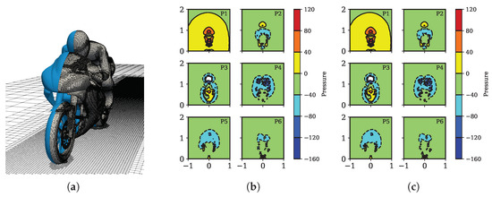
Figure 2.
Contour plots of the pressure variations across different equally-spaced cross-sections of the studied case. Mesh size: M (18 M cells). (a) Computational mesh (M); (b) CPU; (c) GPU.
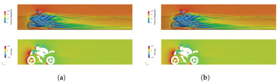
Figure 3.
Contour plots of pressure and velocity fluctuations in the symmetry plane of the investigated case. Mesh size: M (18E6 cells). (a) CPU and (b) GPU. Pressure is denoted as the pressure differential relative to the ambient atmospheric pressure.

Table 1.
Quantitative results for the motorbike test case using the same mesh discretization. Legend: is the drag coefficient, is the lift coefficient, represents the moment coefficients over x, y, and z, and is the side force coefficient.
Considering the objective of this section to assess the consistency of the results between the two methods, the focus is not directed towards the specific physical quantities acquired or the intricacies of modeling choices. Instead, a conventional aerodynamic simulation configuration is adopted, with the primary aimed of examining deviations and computational speed enhancements.
Furthermore, the focus of this study was to compare the performance of a solitary CPU node with that of a single GPU card. This approach was chosen to isolate and evaluate the speedup attributed to a singular GPU card. Notably, the software configuration allows for scalability, making it possible to accommodate larger core counts and operations across multiple GPU cards. Subsequently, the wall clock times presented for each simulation pertain to 1000 steps. Strong linear scaling as calculated by Amdahl’s Law was evident in nearly all conducted tests, a finding corroborated by both CPU and GPU computations.
In Equation (21), s is the speedup attained by parallelizing a program, denotes the execution time of the program when utilizing a single processor, and represents the execution time of the program when employing p processors or cores.
The results of the parallel efficiency experiment are reported in Table 2. The definition of parallel efficiency used here is
Table 2.
Strong scaling analysis for the three tested grids. In this context, “nProcs” refers to the number of CPU cores used to decompose the computational domain.
From Figure 4, it is apparent that the offloaded solution of the pressure equation on the GPU card promotes a roughly two-fold speedup in all the tested cases. As expected, the larger the grid size, the stronger the speedup, as the calculation is computationally more intensive and the weight of the data transfer is proportionally less important. The data illustrated in Figure 4 reveal that transferring the solution of the pressure equation to the GPU yields a more then two-fold speed enhancement compared to employing the PCG solver on the CPU. As expected, this speedup effect becomes more pronounced with increasing grid sizes. This observation aligns with the projected outcome, as larger grids entail more intricate calculations, thereby reducing the relative impact of data transfer. However, in the case of the Geometric Algebraic Multi Grid (GAMG), substantial performance gains were not evident. This can be attributed to the differing solver technology; while the AMG solver within AmgX is directly constructed from the sparse system matrix, OpenFOAM’s geometric multigrid (GAMG) relies on information about the underlying geometric mesh. Consequently, their efficiencies differ. Thus, the comparison between these two solvers encompasses both hardware technology and considerations pertaining to the solver formulations.
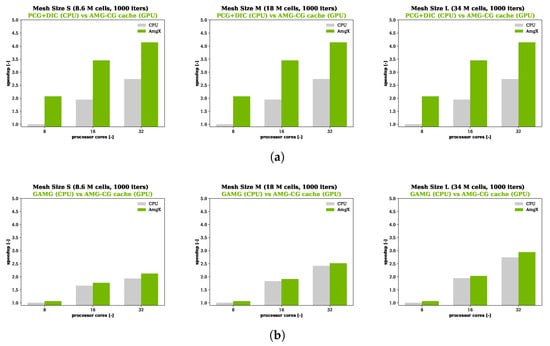
Figure 4.
Strong scalability (Ahmdal’s Law) calculated across three tested grids (S, M, L). The simulation conducted with eight CPU cores served as the reference benchmark. (a) PCG-DIC (CPU) vs. AMG-PCG (GPU) and (b) GAMG (CPU) vs. AMG-PCG (GPU).
The speedup demonstrated in Figure 4 has the potential to increase further, particularly when the pressure equation is iteratively solved multiple times within each iteration of the solver. This scenario arises when mesh non-orthogonality correctors are used. Such instances are common in simulations with strongly non-orthogonal grids or in unsteady simulations employing transient solvers. In the latter case, the pressure equation is solved a minimum of twice per time step.
4. Reactive Flows/Combustion Simulations
Another efficient use of accelerators can be achieved in the context of CFD multiphysics, where improved code performance can be achieved by moving relevant compute-intensive operations to GPUs used as co-processors. This is particularly beneficial when handling large-scale simulations with subproblems involving Ordinary Differential Equations, as in Fluid–Structure Interaction (FSI), Lagrangian Particle Tracking (LPT), and (as will be shown in this case) reactive flow/combustion simulations. The different characteristics and properties of the subproblems to be solved in reactive flows with finite-rate chemistry pose great challenges in the efficient treatment of the highly nonlinear partial differential equations (PDEs) to describe the evolution of reacting flows. In solvers using the operator splitting technique, the solution process is divided into separate problems, specifically, the fluid transport and the chemical mass action. For each Control Volume (CV), the chemical kinetics are integrated over the specified time step as a system of +1 stiff ordinary differential equations (ODEs) to compute the reaction rates and the heat released by the reactions. The results from the fluid transport and the chemical mass action are finally combined to provide the overall solution.
Several algorithmic developments to speed up the solution of ODEs in reactive CFD solvers have been presented over the years in the form of reduction [43,44], tabulation [45,46], and Artificial Neural Network-based strategies [47,48,49]. Their success in finite-rate chemistry compared to Direct Integration (DI) is due to their speed, in particular when dealing with detailed mechanisms. On the other hand, they usually require extensive preprocessing operations [50] or case-dependent tuning of user-input parameters, which is not required with DI. Heterogeneous GPGPU computing potentially represents a very effective solution to accelerate the DI of chemistry problems, which can be solved on accelerators (GPU) while the fluid transport and turbulence are computed using conventional CPU-based hardware technologies. However, such a strategy requires significant redesign, i.e., software co-design [51,52].
4.1. Governing Equations
In addition to the governing equations for fluid flow described in Section 2, a set of convection–diffusion partial differential equations (PDEs) is solved to determine the local mass fraction of each of the chemical species transported by the reactive fluid mixture in each Control Volume (CV):
The mass fraction of the inert species is determined as follows:
In Equation (23), is the mass diffusion coefficient; in reactive simulations, is defined as
where the reaction rate of the i-th specie is
and is scaled by a specific set of coefficients depending on the selected combustion model to eventually account for the interaction between turbulent mixing and chemistry in the CV. With laminar combustion, the laminar finite rate model is used, and = 1 in Equation (25). In Equation (26), is the molecular weight of the i-th species, is the i-th species stoichiometric coefficient, and is the non-equilibrium reaction rate of the j-th reaction:
In Equation (27), and are the forward and reverse rate constants, respectively, at the local fluid dynamic conditions [53], while the ratio is the molar concentration of the i-th species, which in the following is named :
The heat released by the combustion is finally obtained as
where is the enthalpy of formation.
The solution of the chemical mass action (finite-rate chemistry problem) before the flow transport is solved separately for each CV. Reaction rates from calculations of the finite-rate chemistry are passed to the fluid transport problem (Figure 5) as a source term in the species transport equations (Equation (23)). The reaction rate is used by the combustion model to compute the source term (Equation (29)), which in turn is added to the energy equation. In this work, finite-rate chemistry computations are performed on single or multiple Graphical Processing Units (GPUs). Transport properties such as the mass diffusion coefficients, thermal conductivity, and viscosity of the species, along with thermochemical data for the gas phase, are imported from the Cantera transport database through the in-house canteraToFoam utility developed by the authors. As shown in Figure 5, the GPU solver for the finite-rate chemistry can be coupled to any solver available in OpenFOAM, regardless of whether it is pressure-based or density-based. In the following, a shock-capturing density-based solver for the solution of supersonic flows, chosen due to the physics simulated in the validation tests, is used for the fluid transport.
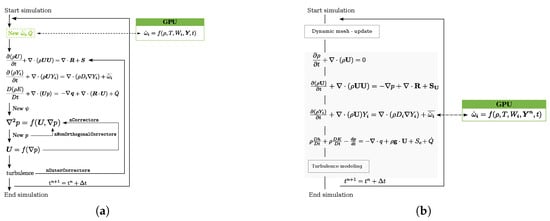
Figure 5.
Solution methods employed in the GPGPU compressible unsteady reactive flow solvers: (a) pressure-based SIMPLE type and (b) density-based shock-capturing type. The calculation of the chemical mass action at each time step is performed on the GPUs.
4.2. Multi-Cell Approach to Accelerating the Chemical Solution on Hybrid CPU–GPU Systems
Combustion simulations with finite-rate chemistry involve the solution of a chemical kinetics system of ordinary differential equations (ODEs). The cost of the computation is proportional to the number of species, number of reactions, and number of grid points in the domain. Nonlinearity in the formulation of reaction rate variables and the contemporary presence of species with very different characteristic time scales leads to very stiff ODE systems; the smallest scales control the size of the integration time step to ensure convergence of the solution, which can significantly impact the computational cost. The time step of integration of the Partial Differential Equations (PDEs) describing the fluid transport problem must comply with the CFL condition, while the integration of the ODE system of the kinetic problem is performed over a time interval that must ensure computational stability [54]. If , a time step subcycling strategy is used and the reaction rate is computed over , as follows:
Here, is the molar concentration of the i-th species at and is the concentration at . The updating of the species concentration in the CV from time n to is computed by the selected ODE integrator. It is important to note that chemistry integration for each CV is assumed to occur for a fixed mass of fluid at a constant pressure; therefore, both the density and volume are changed during integration. When species source terms are computed, they must relate exactly to the mass of fluid considered during integration in order for mass to be conserved; this is achieved by multiplying the mass fractions that results from integration by the old-time density, as it relates to the mass in the cell volume. As a consequence, chemistry integration over a given time step does not depend on the new-time properties of the fluid.
Implicit ODE solvers relying on variable-coefficient methods usually have the best performance for the integration of the finite-rate chemistry problem, as they are capable of extending the time step if the fast modes of the ODE system have already reached their asymptotic values. Conversely, while explicit solvers are characterized by smaller integration time-steps, they avoid the iterative solution and associated matrix inversions required for implicit integration, meaning that they have an intrinsically parallel nature. Therefore, they are well-suited to massive parallel GPU architectures that are optimized to perform a large number of independent operations repeated multiple times. Additionally, their locality reflects on memory usage [55], which is very low compared to implicit solvers. In this work, explicit RK methods with adaptive time-stepping [56] have been selected to solve the ODE system. Embedded Runge-Kutta formulas [57,58] have several advantages: (a) they can be used to construct high-order accurate numerical methods by few evaluation functions and (b) their truncation error can be easily estimated and used to compute the next step size.
The explicit Runge-Kutta Cash–Karp method (Equation (32)) linked to the butcher tableau [59] of Table 3 has been implemented in CUDA. Inputs of the integration algorithm are flow conditions and the global time step of integration. By considering
for a vector of variables under the assumption of isobaric integration ( 0) within the time interval , we have
Table 3.
Runge-Kutta Cash–Karp extended Butcher tableau (right) with reference notation (left).
For each step in Equation (32), an update is needed. An error for each variable in (chemical mass fractions and temperature) is computed at the end of the procedure shown in Equation (32):
here is the difference between the 5th and 4th order solutions. With reference to Table 3, .
Finally, the maximum error
is determined. Equation (33) is calculated locally in the computational cell; thus, convergence is local to each GPU block and the GPU calculation is asynchronous. This limits the synchronization overhead and promotes the maximization of hardware performance. As soon as the kernel calculation is over, the reaction rates and time step advancement for each cell are first stored in the global GPU memory and then copied back to the CPU host. In reactive flow simulations, the GPU solutions are eventually updated (on CPU) by the flow solver. Because the solution of the chemistry is decoupled from the fluid transport, the novel GPU–ODE chemistry integrator can be combined with any flow solver (compressible, incompressible, multiphase) in which the operator splitting technique is applied. As shown in Figure 6, there are three levels of tasks in the CUDA framework, namely, the grid, block, and thread. The grid is made up of several blocks, which are lunched by a GPU kernel. Blocks can be handled asynchronously by the same Streaming Multiprocessor (SM); as all the resources between blocks are shared, communication among blocks is expensive. Each block can execute a certain number of threads. There is only a lightweight synchronization overhead between the threads in a block. All threads in a block run in parallel in the Single Instruction Multiple Threads (SIMT) mode [60]; more precisely, each block contains multiples of 32 threads called warps. Threads in a warp are executed concurrently on a multiprocessor. Modern general-purpose GPUs have a large amount of (slow) global memory and a small amount of (fast) shared memory. Best practice guidelines to improve the performance of a GPU solver suggest (a) saturating the GPU with computational work and balancing the load among all the threads; b) reducing data transfer/communication between the CPU and GPU as much as possible; and (c) limiting threads’ access to the global memory where possible. The chemistry solver presented in this work addresses several of these issues based on profiling outputs. Load balancing, communication overhead, latency, synchronization overhead, and data locality are important factors that may affect performance. To hide latency, asynchronous GPU/CPU data transfer is adopted. To reduce the synchronization overhead, the number of tasks running asynchronously should be maximized. To reduce data transfer, the use of shared memory is rather critical [61], as it limits the threads’ access to the global memory and favors an increase in the efficiency of the algorithm; however, it may lead to divergence of threads [62]. To avoid thread divergence, the code has been written in branchless form. Moreover, because of its limited size, the chunk of GPU shared memory is dynamically allocated at the beginning of the simulation and is used by the GPU for the progressive explicit updating of chemical concentrations and temperature, calculation of the production/consumption rate, and determination of the maximum error. For the methodology proposed in this work, the fat thread approach [63] has been applied, which has several effects on data structure and organization. Data access time is minimized by relying on shared memory and registers, as the data required by the threads are stored. To reduce the communication overhead of data transfers between the CPU and GPU, time-dependent quantities are stored in the dynamic global memory, accessed in a coalesced manner, and progressively stored in chunks of shared memory for the amount of time needed for their use; these are defined as dynamic data. Conversely, constant data are stored when the constant memory is allocated, i.e., at the beginning of the simulation only. The molecular weights of the species, stoichiometric coefficients and exponents of the reaction mechanism, ODE solver settings, and parameters of the Butcher tableau are initialized on the host and then copied and stored in the GPU’s constant memory. The settings of the ODE solver include solution controls (tolerances and maximum number of iterations), scaling factors, and time scaling controls. Time-varying quantities are copied in the GPU’s cached global memory. Thanks to the optimization of the memory access time and latency from the threads, the fat thread approach is very fast, allowing double parallelization of the chemistry problem to be achieved: the ODE system is solved in parallel for the computational cells (on CPUs, this operation is performed serially), and for each computational cell (i.e., block), each species in the reaction mechanism is handled in parallel on multiple active threads (Figure 6). If the amount of data to be transferred overcomes the maximum memory availability of the GPU(s), the chemical problem is automatically split into mesh chunks, each containing a cluster of cells. If the mesh dimension overcomes the maximum number of cells that can be concurrently treated by the GPU streaming multiprocessors, a queue is automatically generated and the overall computational lag and latency is limited thanks to asynchrony. In addition, a GPU block-level control over the cells is used to avoid unnecessary operations. Chemically reactive cells are identified through their local temperature, which must be higher than a given threshold. No ODE integration is performed on the other cells, which are cast off. Finally, the chunk of memory allocated for each GPU block is freed as soon as the relative ODE system is solved in order to move on to handling another cell.
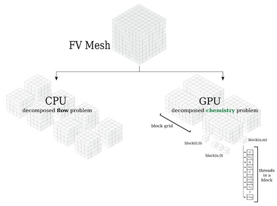
Figure 6.
Decomposition method for hybrid CPU/GPU computations. The heterogeneous solver employs three-level parallelization on the fluid dynamic problem, the chemistry problem, and the reaction mechanism.
4.3. Further Notes about Domain Decomposition in Heterogeneous CPU/GPU Systems
The GPU ODE solver is dynamically linked to the reactive flow solvers available in the open-source software OpenFOAM (Figure 6). Two independent partitionings have been applied to the chemistry problem and the flow domain, respectively. The computational mesh is decomposed into a series of ordered subgroups by a parallel domain decomposition algorithm over the available CPU processor cores. This procedure involves the use of MPI libraries, and is completely independent of the subsequent treatment of the chemistry ODE system. Memory allocation for the transfer of data to the device is produced automatically, ensuring correct memory allocation for each processor based on the available dynamic memory at the beginning of the simulation. Each CPU processor solves the fluid transport, energy, and species transport equations over the assigned subdomain mesh. Multiple GPU cards are managed as a whole and data are synchronized prior to the solution of the fluid transport. At the GPU level, decomposition of the chemical problem is performed independently and relies on a double subdivision over blocks and threads. In particular, each cluster of cells is represented by a series of blocks in which the chemistry problem is solved in parallel; for each block, the solution of the reaction mechanism is parallelized over multiple threads. As a result, double parallelization of the calculation of the chemistry problem on cells/blocks and on species/threads is achieved. As such, three-level parallelization is globally employed, as shown in Figure 6: (a) parallelization of the fluid dynamic problem over CPU processor cores/mesh subdomains; (b) simultaneous solution of the chemistry problem over clusters of cells; and (c) simultaneous/parallel solution of the reaction mechanism in the block threads. The limit on the maximum number of threads per block can be a potential bottleneck for parallelism. This is usually not the case in reactive unsteady CFD simulations, where a 1024-species mechanism is considered a very large mechanism to be solved at run-time. For problems involving larger numbers of species (over a thousand), the thin thread approach [64] is preferred.
4.4. Validation and Verification
The reaction mechanisms were subjected to testing across multiple chosen cases for computations. These cases included:
- -
- Auto-ignition in a single-cell batch reactor. This assessment aimed to verify the solution of Direct Integration (DI) of kinetic mechanisms without considering fluid transport calculations. The GPGPU algorithm’s performance was juxtaposed with two alternatives: (a) an equivalent CPU version of the ODE solver already present in OpenFOAM [31,32] and (b) the solution obtained from Cantera software [65]. This set of simulations was designed to assess the influence of data transfer latency on the overall computation time and to showcase that the various ODE solvers utilized yielded similar results, facilitating a fair comparison.
- -
- Reactive flow simulations on multi-cell domains. This evaluation targeted the holistic performance of the GPGPU solver within the context of fluid transport in the presence of multi-domain parallelization. The validation test cases encompassed the simulation of a scramjet engine.
Chemical kinetics and polynomials describing the thermodynamic properties of the species have been converted from the Cantera format using an in-house developed tool canteraToFoam. All calculations on the GPUs were performed in double precision.
4.5. Auto-Ignition in Single-Cell Batch Reactors
To ensure the accuracy of the CPU/GPU method in solving chemical ODE systems, we utilize direct integration of kinetic mechanisms within single-cell batch reactors. This involves comparing solutions generated by the hybrid CPU/GPU code with those from Cantera [65]. This comparison was conducted for each mechanism under study.
Starting from initial conditions, data synchronization between the CPU and GPU occurs at every integration time step (see Figure 7). However, this synchronization is primarily relevant when fluid transport equations are present. In cases involving single-cell batch reactors, where such equations are absent, this synchronization step becomes unnecessary. On the other hand, it is kept in this context to include the non-negligible time required for data transfer in the estimation of the overall integration time.
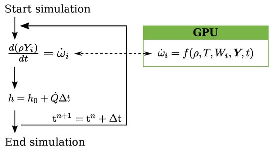
Figure 7.
Solution of autoignition in single-cell batch reactors using a GPGPU solver.
The following quantities were monitored in the simulations:
- -
- The spatial distribution of temperature and species mass fraction;
- -
- The computational time required by the calculation;
- -
- The cumulative mass fraction of the chemical species:
The averaged time integral values of are used to calculate the error of the solution against Cantera [65], which is assumed as the “reference”.
Finally the difference of the results between the GPU and CPU is calculated as:
Hydrogen Combustion. The initial set of computations pertains to a stoichiometric hydrogen–air mixture undergoing reactions at a constant pressure of 2.0 bar and an initial temperature of 1000 K. The mechanism encompasses 10 species and 27 reactions [66]. The absence of stiffness results from both the specific chemistry considered and the utilization of a small global time step.
In Figure 8, the temporal evolution of the temperature and mass fraction of the intermediate species is comparably depicted for both the CPU and the hybrid CPU/GPU solver. The differences in solutions computed by these distinct methods are notably minimal, as demonstrated in Figure 8 and Figure 9. Discrepancies against the reference solution from Cantera (as indicated in Equations (36) and (37)) are presented for each of the monitored species in Figure 9a.
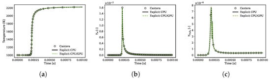
Figure 8.
Hydrogen/air auto-ignition predicted over time by the direct integration of the chemistry problem on the hybrid CPU/GPU code by an explicit CPU solver and by Cantera [65]. (a) temperature; (b) evolution in time of ; (c) evolution in time of .
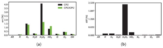
Through this testing, it is observed that the maximum relative discrepancy in GPU integration remains below 2%, while the highest relative discrepancy encountered in the CPU is 4%. This outcome underscores the strong agreement and limited variations between the hybrid CPU/GPU solver and the CPU counterpart.
4.6. Validation Test: Supersonic Combustion in a Scramjet Engine
The three-dimensional simulation of supersonic combustion in a scramjet engine by the DLR combustor facility [67,68,69] was used to validate the proposed GPGPU solver. The geometrical features of the scramjet engine geometry are reported in [70,71,72] and summarized in Figure 10. The configuration consists of a one-sided divergence channel that confines preheated air and a wedge-shaped flame stabilizer. The upper wall diverges to compensate for the expansion of the boundary layer.
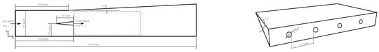
Figure 10.
Geometry of the scramjet test case [67,68,69]. In the experimental setup, a transparent window for high-speed camera visualizations is located in the region marked by the red dashed line.
Fuel injection occurs from the reference origin along the x direction. Each fuel injection hole has a diameter of 1 mm, and each of the 15 circular holes is separated by 2.4 mm [70,71,72].
The boundary conditions of the problem are summarized in Table 4. Fixed values of pressure, velocity and temperature are set at the air and fuel inlets. The inlet air enters the domain with Ma = 2. It is preheated and includes a fraction of water in gaseous form. Hydrogen is injected by the circular fuel inlets at Ma = 1. The chamber and wedge walls are adiabatic. In the literature, the combustor has been analysed considering one [70,72], three [71], and five [71] of the fifteen injectors, while neglecting the effects of the side walls. In the current study, the three-nozzle configuration [71] has been considered. The boundary layers of the upper and lower walls are not resolved [70], as this aspect was out of scope for the present work and requires further study.
Table 4.
Physical boundary conditions for the operation of the scramjet engine [70,71,72].
The computational domain is reported in Figure 11. In regions with large temperature gradients, Adaptive Mesh Refinement (AMR) is dynamically applied at run-time to the initial body-fitted hexahedral mesh of 1.5 M cell elements. The flow field was initialized by a precursor cold-flow simulation to reproduce the complex shock wave pattern (duration s), and the duration of the reactive simulation is s. A hot spot in the recirculating region is set to ignite the mixture.
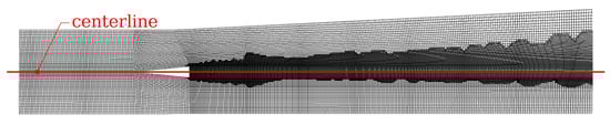
Figure 11.
Body-fitted hexahedral Finite Volume (FV) mesh of the scramjet engine. Adaptive Mesh Refinement (AMR) is dynamically applied at run-time in proximity to large temperature gradients between neighboring cells. The number of cell elements ranges between 1.5 M (initial mesh) and 15 M.
4.7. Simulation of Supersonic Combustion in the Scramjet Engine
Beginning with the flow field established through an initial cold-flow simulation, subsequent calculations were performed to simulate reactive flows. The dynamic evolution within the reactive region induces modifications in the shock pattern downstream of the structural injector. The emergence of recirculation regions promotes flame stabilization. Upon impingement on the structural element, the supersonic flow generates two oblique shocks that subsequently interact with the upper and lower walls, rebounding towards the central area. The core flow at the center experiences heightened turbulence due to ongoing combustion. Consequently, the previously orderly shock wave pattern in the far region of the combustor becomes disrupted as the core region expands. For validation, a comparative analysis is presented in Figure 12 between an experimental Schlieren image and the corresponding numerical density gradient plot from the reactive simulation. The visualization window in Figure 12 corresponds to the region delineated by the red dashed line in Figure 10. The comparison reveals satisfactory agreement in both the evolution and enlargement of the core region.
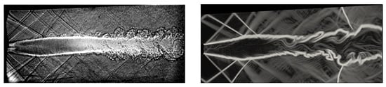
Figure 12.
Comparison of density gradients for the hot simulation: Schlieren image [70] (left) vs. numerical solution (right).
The behaviour of the pressure at the base largely varies when compared to the nonreactive case. The pressure slightly increases (see Figure 13) and the core wake becomes quasi-parallel to the freestream flow, as observed in [70,73]; thus, only small waves are observed further downstream. From this, it can be derived that only small variations in pressure are experienced towards the outlet of the combustor.
Figure 13.
Pressure distribution at the bottom wall for the reactive flow simulation: comparison between simulations and experiments [70]. Legend: Menon ( ) [70]; Fureby (
 ) [73]; CPU (
 ).
).
) [70]; Fureby () [73]; CPU ().
Flow temperature was investigated quantitatively by comparing coherent anti-Stokes Raman spectroscopy solutions at x = 11 mm, 58 mm, and 166 mm (Figure 14). The temperature peaks predicted at the first location are slightly higher than the measured counterparts, while the symmetric profile of the experiments is correctly captured. A better agreement is appreciable downstream (Figure 14b,c), even though the region where combustion takes place is slightly larger than the experimental one (Figure 14b). The reactive simulation was run once more using the GPU–ODE integrator, thereby exploiting a heterogeneous application. The results in green shown in Figure 14 confirm the good agreement with the full-CPU solutions used as a reference.
Figure 14.
Mean temperature (K) at different positions along the flowpath: (a) x = 11 mm; (b) x = 58 mm; (c) x = 106 mm.
Finally, Figure 15 (upper line) reports the temperature flow distribution within a threshold, and is used to highlight the shape of the flame at two different timesteps. The shape of the flame clearly highlights the presence of flow instabilities and small recirculating regions at the interface. Large recirculation vortices are present within the core region; these are generated behind the struct and carried towards the end of the domain as they evolve. The penetration of the fuel jet is lower than in the nonreacting case. Again, it is clear that the the shear layer instabilities generated at the corners of the flame stabilizer do not converge toward the centerline, instead interacting with the recirculation bubble behind the struct.
Figure 15.
Combustion simulation at two different time steps, showing a representation of the flame via the threshold (top) and density field (bottom): (a) s; (b) s.
4.8. Performance
Scalability testing of the reactive simulations by the GPGPU solver was investigated considering the initial coarse mesh used for the supersonic test case over a span of the first 100 time steps (including the time to read the mesh from disk). As the AMR was not active in this test, the grid counted a limited number of cells (1.5 M). Unlike the cases including flow transport only, the computational load in reactive flow simulations is mostly provided by the solution of the finite rate chemistry, e.g., the size of the kinetic mechanism, rather than by the mesh size. The scalability for the cold flow simulation, e.g., without finite-rate chemistry calculations, is linear only within a limited range up to about 24 cores (see Figure 16a). The same holds if chemical species are tracked without reactions (Figure 16b). Finally, if combustion with finite-rate chemistry is triggered, the computational load increases. This is because (a) the number of convection–diffusion equations is larger due to the tracking of the intermediate species and (b) the solution of finite-rate chemistry ODEs is now active. In this case, linear scalability is preserved for a higher number of cores (Figure 16c).
Figure 16.
Scalability of the reactive flow solver on the initial coarse mesh (1.5 M cells, AMR deactivated): (a) cold flow simulation; (b) cold-flow simulation with species-transport (combustion off); (c) reactive flow simulation with finite-rate chemistry calculations.
Scalability testing of the GPGPU solver for reactive simulations was conducted, focusing on the initial coarse mesh utilized in the supersonic test case for the first 100 time steps (inclusive of mesh reading time). For this test, Adaptive Mesh Refinement (AMR) was not active, resulting in a limited cell count of 1.5 million.
In contrast to cases involving flow transport alone, the computational load in reactive flow simulations is primarily determined by the solution of the finite-rate chemistry, e.g., the size of the kinetic mechanism used, rather than the mesh size. Scalability in cold flow simulations without finite-rate chemistry calculations demonstrates linear behavior only within a restricted range up to approximately 24 cores, as shown in Figure 16a. The same linear trend is observed when tracking chemical species without reactions (Figure 16b).
However, when combustion with finite-rate chemistry is introduced, the computational load increases, which is due to two factors: (a) the greater number of convection–diffusion equations resulting from tracking intermediate species and (b) the active involvement of finite-rate chemistry ODE solutions. In this scenario, linear scalability is sustained over a broader range of cores (Figure 16c).
Let tCPU and tGPU represent the respective computation times for solving the finite-rate chemistry problem on the CPU and GPU. Additionally, we define tf,GPU as the time required for GPU memory allocation, CPU data collection, and the forward data transfer (CPU-to-GPU), tk,GPU as the time for the kernel call and actual ODE integration on the GPU, and as the duration for completing the backward data transfer (GPU-to-CPU). The use of GPGPU solver is advantageous if
From Equation (39), it is evident that the speedup resulting from the vectorization employed by the GPU during chemistry problem calculations becomes increasingly advantageous as the problem size expands.
In the context of reactive flow simulations, utilizing the GPGPU solver with 24 cores and an NVIDIA Tesla V100card demonstrates a 9.3× improvement in speed compared to the same solver running exclusively on 24 CPU cores. The developed GPGPU solution inherently supports computations across multiple nodes and GPU cards. The tests presented herein were conducted using a single GPU to examine its operational behavior.
5. Conclusions
Our focus in this study centered on the synergies between numerical methods and the code architecture within Finite Volume (FV) software, with the aim of devising accelerated algorithms to enhance Computational Fluid Dynamics (CFD) simulations encompassing governing equations and submodels for combustion chemistry. We demonstrate that leveraging GPUs for solving the linear algebra of Partial Differential Equations (PDEs) proves particularly advantageous in a segregated solver, especially when applied to the most computationally intensive equation, namely, the pressure equation. The extent of this advantage becomes even more pronounced if the pressure equation is iteratively solved multiple times within each iteration of the solver. This scenario arises when dealing with mesh non-orthogonality correction or in transient simulations employing a transient solver. The efficiency gain brought about by GPUs in solving linear algebra is remarkably satisfactory, as observed in comparisons with similar solver technologies. On another note, fully exploiting GPUs’ potential for CFD necessitates executing a coupled matrix assembly with the entire code running directly on the GPU(s). Such an approach could significantly minimize data transfer time and harness the substantially parallel architecture of GPUs. This aspect of our work is presently in the development phase.
A second part of this investigation pertained to accelerating Ordinary Differential Equation (ODE) solvers, which are commonly employed in multiphysics problems. A specific case is that of reactive/combustion CFD simulations. In solvers predicated on the operator splitting technique, the scalability of the solver is interconnected with the resolution of two distinct subproblems, namely, linear algebra and ODEs. By offloading computationally intensive operations to GPUs a nearly ten-fold acceleration was achieved in simulations, causing the scalability range to shift towards a higher core count.
Author Contributions
Conceptualization, F.P. and F.G.; methodology, F.P. and F.G.; software, F.P. and F.G.; validation, F.P. and F.G.; formal analysis, F.P. and F.G.; investigation, F.P. and F.G.; resources, F.P. and F.G.; data curation, F.P. and F.G.; writing—original draft preparation, F.P. and F.G.; writing—review and editing, F.P. and F.G.; visualization, F.P. and F.G.; supervision, F.P.; project administration, F.P.; funding acquisition, F.P. All authors have read and agreed to the published version of the manuscript.
Funding
This work has received funding from the European High-Performance Computing Joint Undertaking (JU) under Grant Agreement No 956416 (project: exaFoam [9]). The JU receives support from the European Union’s Horizon 2020 Research and Innovation Programme, as well as from France, the United Kingdom, Germany, Italy, Croatia, Spain, Greece, and Portugal.
Acknowledgments
The authors gratefully acknowledge the Laboratory Computing Resource Center (LCRC) at Argonne National Laboratory (Lemont, US) for the computing resources provided. Special thanks are extended to the OpenFOAM HPC Technical Committee and ESI-OpenCFD Ltd. for their invaluable contributions through constructive technical discussions during the development and testing phases of this study.
Conflicts of Interest
The authors declare no conflict of interest.
Appendix A. Link between Density and Pressure Correction
The link between density correction and pressure correction is provided by
where
is the compressibility of the fluid; with
it follows that
Appendix B. Link between Veocity and Pressure Correction
At the m-th outer iteration within the time step integration from time n to n+1, the momentum equation can be written as
In addition, the corrected velocity and pressure must satisfy
References
- Resolved Analytics, CFD Software Comparison. Available online: https://www.resolvedanalytics.com/theflux/comparing-cfd-software (accessed on 15 August 2023).
- NVIDIA. The Computational Fluid Dynamics Revolution Driven by GPU Acceleration. Available online: https://developer.nvidia.com/blog/computational-fluid-dynamics-revolution-driven-by-gpu-acceleration/ (accessed on 10 August 2023).
- Kiran, U.; Sharma, D.; Gautam, S.S. GPU-warp based finite element matrices generation and assembly using coloring method. J. Comput. Des. Eng. 2019, 6, 705–718. [Google Scholar] [CrossRef]
- Accelerating ANSYS Fluent using NVIDIA GPUs, NVIDIA. 2014. Available online: https://www.nvidia.com/content/tesla/pdf/ansys-fluent-nvidiagpu-userguide.pdf (accessed on 11 August 2023).
- Siemens Digital Industries Software. Simcenter STAR-CCM+, version 2023; Siemens: Munich, Germany, 2023. [Google Scholar]
- Martineau, M.; Posey, S.; Spiga, F. OpenFOAM solver developments for GPU and arm CPU. In Proceedings of the 18th OpenFOAM Workshop, Genova, Italy, 11–14 July 2023. [Google Scholar]
- Piscaglia, F. Modern methods for accelerated CFD computations in OpenFOAM. In Proceedings of the Keynote Talk at the 6th French/Belgian OpenFOAM Users Conference, Grenoble, France, 13–14 June 2023. [Google Scholar]
- Ferziger, J.H.; Perić, M.; Street, R.L. Computational Methods for Fluid Dynamics, 4th ed.; Springer: Berlin/Heidelberg, Germany, 2020. [Google Scholar]
- exaFoam EU Project. Available online: https://exafoam.eu/ (accessed on 6 August 2023).
- The European Centre of Excellence for Engineering Applications (EXCELLERAT P2). Available online: https://www.excellerat.eu/ (accessed on 6 August 2023).
- Ghioldi, F.; Piscaglia, F. GPU Acceleration of CFD Simulations in OpenFOAM. In Proceedings of the 18th OpenFOAM Workshop, Genova, Italy, 11–14 July 2023. [Google Scholar]
- Wichman, I.S. On the use of operator-splitting methods for the equations of combustion. Combust. Flame 1991, 83, 240–252. [Google Scholar] [CrossRef]
- Descombes, S.; Duarte, M.; Massot, M. Operator Splitting Methods with Error Estimator and Adaptive Time-Stepping. Application to the Simulation of Combustion Phenomena. In Splitting Methods in Communication, Imaging, Science, and Engineering; Springer International Publishing: Cham, Switzerland, 2016; pp. 627–641. [Google Scholar] [CrossRef]
- Yang, B.; Pope, S. An investigation of the accuracy of manifold methods and splitting schemes in the computational implementation of combustion chemistry. Combust. Flame 1998, 112, 16–32. [Google Scholar] [CrossRef]
- Singer, M.; Pope, S.; Najm, H. Modeling unsteady reacting flow with operator splitting and ISAT. Combust. Flame 2006, 147, 150–162. [Google Scholar] [CrossRef]
- Ren, Z.; Xu, C.; Lu, T.; Singer, M.A. Dynamic adaptive chemistry with operator splitting schemes for reactive flow simulations. J. Comput. Phys. 2014, 263, 19–36. [Google Scholar] [CrossRef]
- Lu, Z.; Zhou, H.; Li, S.; Ren, Z.; Lu, T.; Law, C.K. Analysis of operator splitting errors for near-limit flame simulations. J. Comput. Phys. 2017, 335, 578–591. [Google Scholar] [CrossRef]
- Xue, W.; Jackson, C.W.; Roy, C.J. An improved framework of GPU computing for CFD applications on structured grids using OpenACC. J. Parallel Distrib. Comput. 2021, 156, 64–85. [Google Scholar] [CrossRef]
- Ghioldi, F.; Piscaglia, F.; Ghioldi, F.; Piscaglia, F. A CPU-GPU Paradigm to Accelerate Turbulent Combustion and Reactive-Flow CFD Simulations. In Proceedings of the 8th OpenFOAM Conference, Virtual, 13–15 October 2020. [Google Scholar]
- Ghioldi, F.; Piscaglia, F.; Ghioldi, F.; Piscaglia, F. GPU-Accelerated Simulation of Supersonic Combustion in Scramjet Engines by OpenFOAM. In Proceedings of the 33rd International Conference on Parallel Computational Fluid Dynamics—ParCFD2022, Manhattan, NY, USA, 25–27 May 2022. [Google Scholar]
- Martineau, M.; Posey, S.; Spiga, F. AmgX GPU Solver Developments for OpenFOAM. In Proceedings of the 8th OpenFOAM Conference, Virtual, 13–15 October 2020. [Google Scholar]
- Nagy, D.; Plavecz, L.; Hegedűs, F. The art of solving a large number of non-stiff, low-dimensional ordinary differential equation systems on GPUs and CPUs. Commun. Nonlinear Sci. Numer. Simul. 2022, 112, 106521. [Google Scholar] [CrossRef]
- Jaiswal, S.; Reddy, R.; Banerjee, R.; Sato, S.; Komagata, D.; Ando, M.; Okada, J. An Efficient GPU Parallelization for Arbitrary Collocated Polyhedral Finite Volume Grids and Its Application to Incompressible Fluid Flows. In Proceedings of the 2016 IEEE 23rd International Conference on High Performance Computing Workshops (HiPCW), Hyderabad, India, 19–22 December 2016; pp. 81–89. [Google Scholar] [CrossRef]
- Ghioldi, F. Fast Algorithms for Highly Underexpanded Reactive Spray Simulations. Master’s Thesis, Politecnico di Milano, Milan, Italy, 2019. Available online: https://hdl.handle.net/10589/146075 (accessed on 11 August 2023).
- Trevisiol, F. Accelerating Reactive Flow Simulations via GPGPU ODE Solvers in OpenFOAM. Master’s Thesis, Politecnico di Milano, Milan, Italy, 2020. Available online: https://hdl.handle.net/10589/170955 (accessed on 11 August 2023).
- Ghioldi, F. Development of Novel CFD Methodologies for the Optimal Design of Modern Green Propulsion Systems. Ph.D. Thesis, Politecnico di Milano, Milan, Italy, 2022. Available online: https://hdl.handle.net/10589/195309 (accessed on 11 August 2023).
- Dyson, J. GPU Accelerated Linear System Solvers for OpenFOAM and Their Application to Sprays. Ph.D. Thesis, Brunel University London, Uxbridge, UK, 2016. [Google Scholar]
- Molinero, D.; Galván, S.; Domínguez, F.; Ibarra, L.; Solorio, G. Francis 99 CFD through RapidCFD accelerated GPU code. IOP Conf. Ser. Earth Environ. Sci. 2021, 774, 012016. [Google Scholar] [CrossRef]
- Jacobsen, D.A.; Senocak, I. Multi-level parallelism for incompressible flow computations on GPU clusters. Parallel Comput. 2013, 39, 1–20. [Google Scholar] [CrossRef]
- Naumov, M.; Arsaev, M.; Castonguay, P.; Cohen, J.; Demouth, J.; Eaton, J.; Layton, S.; Markovskiy, N.; Reguly, I.; Sakharnykh, N.; et al. AmgX: A Library for GPU Accelerated Algebraic Multigrid and Preconditioned Iterative Methods. SIAM J. Sci. Comput. 2015, 37, S602–S626. [Google Scholar] [CrossRef]
- The OpenFOAM Foundation. Available online: http://www.openfoam.org/dev.php (accessed on 15 August 2023).
- ESI OpenCFD OpenFOAM. Available online: http://www.openfoam.com/ (accessed on 15 August 2023).
- Caretto, L.S.; Gosman, A.D.; Patankar, S.V.; Spalding, D.B. Two calculation procedures for steady, three-dimensional flows with recirculation. In Proceedings of the Third International Conference on Numerical Methods in Fluid Mechanics; Lecture Notes in Physics; Cabannes, H., Temam, R., Eds.; Springer: Berlin/Heidelberg, Germany, 1973; Volume 1, pp. 60–68. [Google Scholar]
- Gordon, S.; McBride, B. Computer Program for Calculation of Complex Equi- librium Compositions, Rocket Performance, Incident and Reflected Shocks, and Chapman-Jouguet Detonations; NASA Techical Report SP-273; National Aeronautics and Space Administration: Washington, DC, USA, 1971. [Google Scholar]
- Intel one API Math Kernel Library (MKL) Developer Reference. Available online: https://software.intel.com/content/www/us/en/develop/articles/mkl-reference-manual.html (accessed on 15 August 2023).
- Balay, S.; Abhyankar, S.; Adams, M.F.; Benson, S.; Brown, J.; Brune, P.; Buschelman, K.; Constantinescu, E.M.; Dalcin, L.; Dener, A.; et al. PETSc Web Page. 2023. Available online: https://petsc.org/ (accessed on 15 August 2023).
- NVIDIA cuSPARSE Library. Available online: https://github.com/NVIDIA/CUDALibrarySamples/tree/master/cuSPARSE (accessed on 15 August 2023).
- Algebraic Multigrid Solver (AmgX) Library. Available online: https://github.com/NVIDIA/AMGX (accessed on 15 August 2023).
- Barrett, R.; Berry, M.; Chan, T.F.; Demmel, J.; Donato, J.; Dongarra, J.; Eijkhout, V.; Pozo, R.; Romine, C.; van der Vorst, H. Templates for the Solution of Linear Systems: Building Blocks for Iterative Methods; Society for Industrial and Applied Mathematics: Philadelphia, PA, USA, 1994. [Google Scholar] [CrossRef]
- Saad, Y. A Flexible Inner-Outer Preconditioned GMRES Algorithm. SIAM J. Sci. Comput. 1993, 14, 461–469. [Google Scholar] [CrossRef]
- Vogel, J.A. Flexible BiCG and flexible Bi-CGSTAB for nonsymmetric linear systems. Appl. Math. Comput. 2007, 188, 226–233. [Google Scholar] [CrossRef]
- Bna, S. foam2CSR. 2021. Available online: https://gitlab.hpc.cineca.it/openfoam/foam2csr (accessed on 15 August 2023).
- Liang, L.; Stevens, J.G.; Raman, S.; Farrell, J.T. The use of dynamic adaptive chemistry in combustion simulation of gasoline surrogate fuels. Combust. Flame 2009, 156, 1493–1502. [Google Scholar] [CrossRef]
- Goldin, G.M.; Ren, Z.; Zahirovic, S. A cell agglomeration algorithm for accelerating detailed chemistry in CFD. Combust. Theory Model. 2009, 13, 721–739. [Google Scholar] [CrossRef]
- Singer, M.A.; Pope, S.B. Exploiting ISAT to solve the reaction–diffusion equation. Combust. Theory Model. 2004, 8, 361–383. [Google Scholar] [CrossRef][Green Version]
- Li, Z.; Lewandowski, M.T.; Contino, F.; Parente, A. Assessment of On-the-Fly Chemistry Reduction and Tabulation Approaches for the Simulation of Moderate or Intense Low-Oxygen Dilution Combustion. Energy Fuels 2018, 32, 10121–10131. [Google Scholar] [CrossRef]
- Blasco, J.; Fueyo, N.; Dopazo, C.; Ballester, J. Modelling the Temporal Evolution of a Reduced Combustion Chemical System With an Artificial Neural Network. Combust. Flame 1998, 113, 38–52. [Google Scholar] [CrossRef]
- Nikitin, V.; Karandashev, I.; Malsagov, M.Y.; Mikhalchenko, E. Approach to combustion calculation using neural network. Acta Astronaut. 2022, 194, 376–382. [Google Scholar] [CrossRef]
- Ji, W.; Qiu, W.; Shi, Z.; Pan, S.; Deng, S. Stiff-PINN: Physics-Informed Neural Network for Stiff Chemical Kinetics. J. Phys. Chem. A 2021, 125, 8098–8106. [Google Scholar] [CrossRef]
- Tap, F.; Schapotschnikow, P. Efficient Combustion Modeling Based on Tabkin® CFD Look-up Tables: A Case Study of a Lifted Diesel Spray Flame. In Proceedings of the SAE Technical Paper; SAE International: Warrendale, PA, USA, 2012. [Google Scholar] [CrossRef]
- Haidar, A.; Brock, B.; Tomov, S.; Guidry, M.; Billings, J.J.; Shyles, D.; Dongarra, J.J. Performance analysis and acceleration of explicit integration for large kinetic networks using batched GPU computations. In Proceedings of the 2016 IEEE High Performance Extreme Computing Conference (HPEC), Waltham, MA USA, 13–15 September 2016; pp. 1–7. [Google Scholar]
- Wilt, N. The CUDA Handbook: A Comprehensive Guide to GPU Programming; Addison-Wesley: Boston, MA, USA, 2013. [Google Scholar]
- Poinsot, T.; Veynante, D. Theoretical and Numerical Combustion, 3rd ed.; CNRS: Paris, France, 2012. [Google Scholar]
- Van Der Houwen, P.; Sommeijer, B.P. On the Internal Stability of Explicit, m-Stage Runge-Kutta Methods for Large m-Values. J. Appl. Math. Mech. 1980, 60, 479–485. [Google Scholar] [CrossRef]
- Volkov, V. Better performance at lower occupancy. In Proceedings of the 2008 ACM/IEEE Conference on Supercomputing, Austin, TX, USA, 15–21 November 2008. [Google Scholar]
- Press, W.; Teukolsky, S.; Vetterling, W.; Flannery, B. Numerical Recipes in C, 2nd ed.; Cambridge University Press: Cambridge, UK, 1997. [Google Scholar]
- Fehlberg, E. Some Experimental Results Concerning the Error Propagation in Runge-Kutta Type Integration Formulas; NASA Techical Report; National Aeronautics and Space Administration: Washington, DC, USA, 1970. [Google Scholar]
- Fehlberg, E. Low-order Classical Runge-Kutta Formulas with Stepsize Control and Their Application to Some Heat Transfer Problems; NASA Technical Report TR-R-315; National Aeronautics and Space Administration: Washington, DC, USA, 1969. [Google Scholar]
- Cash, J.; Karp, A. A Variable Order Runge-Kutta Method for Initial Value Problems with Rapidly Varying Right-Hand Sides. Acm Trans. Math. Softw. 1990, 16, 201–222. [Google Scholar] [CrossRef]
- Nickolls, J.; Dally, W.J. The GPU Computing Era. IEEE Micro 2010, 30, 56–69. [Google Scholar] [CrossRef]
- Lindholm, E.; Nickolls, J.; Oberman, S.; Montrym, J. NVIDIA Tesla: A Unified Graphics and Computing Architecture. IEEE Micro 2008, 28, 39–55. [Google Scholar] [CrossRef]
- Branch Statistics. Available online: https://docs.nvidia.com/gameworks/content/developertools/desktop/analysis/report/cudaexperiments/kernellevel/branchstatistics.htm (accessed on 3 February 2023).
- NVIDIA; Vingelmann, P.; Fitzek, F.H.P. CUDA, Release: 10.2.89. 2020. Available online: https://developer.nvidia.com/cuda-toolkit (accessed on 11 August 2023).
- Klingbeil, G.; Erban, R.; Giles, M.; Maini, P.K. Fat versus Thin Threading Approach on GPUs: Application to Stochastic Simulation of Chemical Reactions. IEEE Trans. Parallel Distrib. Syst. 2012, 23, 280–287. [Google Scholar] [CrossRef]
- Goodwin, D.G.; Speth, R.L.; Moffat, H.K.; Weber, B.W. Cantera: An Object-Oriented Software Toolkit for Chemical Kinetics, Thermodynamics, and Transport Processes. Version 2.4.0. 2018. Available online: https://www.cantera.org (accessed on 15 August 2023). [CrossRef]
- Hong, Z.; Davidson, D.F.; Hanson, R.K. An improved H2/O2 mechanism based on recent shock tube/laser absorption measurements. Combust. Flame 2011, 158, 633–644. [Google Scholar] [CrossRef]
- Guerra, R.; Waidmann, W.; Laible, C. An Experimental Investigation of the Combustion of a Hydrogen Jet Injected Parallel in a Supersonic Air Stream. In Proceedings of the AIAA 3rd International Aerospace Conference, Washington, DC, USA, 3–5 December 1991. [Google Scholar]
- Waidmann, W.; Alff, F.; Bohm, M.; Claus, W.; Oschwald, M. Experimental Investigation of the Combustion Process in a Supersonic Combustion Ramjet (SCRAMJET); Technical Report; DGLR Jahrestagung: Erlangen, Germany, 1994. [Google Scholar]
- Waidmann, W.; Alff, F.; Böhm, M.; Brummund, U.; Clauss, W.; Oschwald, M. Supersonic Combustion of Hydrogen/Air in a Scramjet Combustion Chamber. Space Technol. 1994, 6, 421–429. [Google Scholar]
- Génin, F.; Menon, S. Simulation of Turbulent Mixing Behind a Strut Injector in Supersonic Flow. AIAA J. 2010, 48, 526–539. [Google Scholar] [CrossRef]
- Potturi, A.; Edwards, J. Investigation of Subgrid Closure Models for Finite-Rate Scramjet Combustion. In Proceedings of the 43rd Fluid Dynamics Conference, San Diego, CA, USA, 24–27 June 2013; pp. 1–10. [Google Scholar] [CrossRef]
- Zhang, H.; Zhao, M.; Huang, Z. Large eddy simulation of turbulent supersonic hydrogen flames with OpenFOAM. Fuel 2020, 282, 118812. [Google Scholar] [CrossRef]
- Berglund, M.; Fureby, C. LES of supersonic combustion in a scramjet engine model. Proc. Combust. Inst. 2007, 31, 2497–2504. [Google Scholar] [CrossRef]
Disclaimer/Publisher’s Note: The statements, opinions and data contained in all publications are solely those of the individual author(s) and contributor(s) and not of MDPI and/or the editor(s). MDPI and/or the editor(s) disclaim responsibility for any injury to people or property resulting from any ideas, methods, instructions or products referred to in the content. |
© 2023 by the authors. Licensee MDPI, Basel, Switzerland. This article is an open access article distributed under the terms and conditions of the Creative Commons Attribution (CC BY) license (https://creativecommons.org/licenses/by/4.0/).