Power Balance Strategies in Steady-State Simulation of the Micro Gas Turbine Engine by Component-Coupled 3D CFD Method

Abstract

Currently, an increasing number of designers have begun to pay attention to a new paradigm for evaluating the performance with full engine 3-dimensional computational fluid dynamics (3D CFD) simulations. Compared with the traditional component-based performance simulation method component-based performance simulation method (‘component-matched’ method), this novel ‘component-coupled’ method can evaluate the overall performance of the engine more physically and obtain more detailed flow field parameters simultaneously. Importantly, the power balance iteration should be introduced to the novel method to satisfy the constraints of the coaxial components for the gas turbine engine at steady state. By carrying out the ‘component-matched’ simulation and the ‘component-coupled’ simulation for a micro turbojet engine, the necessity of introducing the power balance iteration was discussed in this paper. The influence of steady-state co-working constraints on the engine performance was analysed and strategies for power balance iteration were proposed. To verify the capability and feasibility of this method, not only the co-working state but also the windmill state of the gas turbine engine were simulated by using the 3D CFD method considering power balance iteration. The results show that the power balance strategy proposed in this paper can converge the aerodynamic parameters as well as the power residual in a robust way.

1. Introduction

As a highly complex thermal system, the physical and chemical processes inside the gas turbine engine should be carefully considered in the design procedure to make all the components felicitously matched. Numerical simulation is an effective way to evaluate the engine performance and obtain the flow field details.

According to the dimension of the mathematical model, the numerical simulation method can be divided into the following four levels: the 0D method based on the thermal cycle and data model of component’s characteristics [1,2]; the 1D method based on ordinary differential equations (ODE) [3,4] or partial differential equations (PDE) [5]; the 2D method based on through-flow theory [6,7,8,9]; the 3D method based on the Navier–Stokes(N–S) equation [10,11,12,13]. Other trans-dimensional methods, otherwise known as multi-fidelity methods, were also reported as the a compromise between low-dimensional (0–2D) and 3D methods [14,15,16]. Although the numerical simulation method based on the low-dimensional models has great advantages in terms of computational efficiency, it relies highly on experimental data, empirical formulas or other remedies to correct the model with the dimensional reduction. In low-dimensional simulations, such as through-flow simulations, the turbulence models used in CFD cannot accurately simulate viscous losses for the dimensional reduction. Therefore, the empirical loss models or viscous force models need to be supplemented for these methods [17,18,19]. Leaving the difficulty of establishing this kind of model aside, the low-dimensional simulation method with nonphysical treatment of the components’ interfaces or boundaries cannot reflect the coupling relationship of the components. Most low-dimensional simulations based on solving the residual equations rather than PDE/ODE cannot consider the downstream-to-upstream transmission of the flow field in the iteration for matching the components of the engine, such as the forward transmission of the heat from the combustion chamber to the compressor [20].

The ‘component-coupled’ simulation method based on 3D CFD can truly reflect the interactions between the components, and obtain the overall engine performance and flow field data more physically trusting. With the explosive growth of computing power, this method based on 3D CFD has broad application prospects. In previous papers, the 3D CFD method has been used to research the combustor-turbine interactions [21,22] and compressor-combustor interactions [23,24]; however only two components were involved in such cases. In this paper, the ‘component-coupled’ simulation stands for the integrated simulation of the full engine with three core components(compressor, combustor and turbine). Different from considering only two adjacent components, the shaft power matching must be considered in this kind of simulation. For the steady-state, this means the simulations not only need to converge the aerodynamic parameters, but also need to meet the power balance of the compressor and the turbine.

Typically, the co-working state parameters, such as the rotation speed and the fuel mass flow, are given as the input parameters. As the definite conditions of the simulation, these co-working state parameters can be obtained by experiments or other evaluation methods. In this way, many previous studies implement the 3D CFD simulation of the full engine with the post-verification of the power balance. In 2006, Stanford University published their simulation of the entire high-spool of the PW6000 gas turbine engine, and the feasibility of a numerical test bench based on 3D CFD was verified [10,11]. This simulation realizes the switching of the turbulence model between Reynolds-Averaged Navier–Stokes (RANS) simulations and Large-Eddy Simulations (LES) based on interface technology. Mentor company [12] carried out the full engine simulation of a micro gas turbine engine using the FloEFD software in 2012. It is pointed out that the combustion chamber will be deformed under the temperature and pressure load, and the displacement can reach 0.001 m. In 2013, Imperial College London in cooperation with Rolls-Royce carried out a simulation of the full engine with AU3X code [25]. It is reported that the total temperature and total pressure error at the key section was less than 5%. Samara State Aerospace University used ANSYS CFX to simulate the performance of a small gas turbine engine, and compared it with the 1D calculation results of the ASTRA program [26]. The simulation results show that there is a torque deviation of 5% between the compressor and the turbine. The above simulation can only verify the power balance between compressor and turbine after the aerodynamic parameters converge, and the posterior error may be large. Actually, the magnitude of the power balance residual is mainly determined by the definite condition of the simulation.

To reduce the power balance residual and extend the usefulness of the 3D CFD engine simulation, the automatic power balance iteration should be introduced. Based on the Trilinos package, researchers developed a 3D engine simulation program [27]. In this CFD solver by automatically adjusting the definite condition, the power balance of the engine was realized. Teixeira et al. carried out a single-channel RANS simulation of a micro gas turbine engine using NUMECA software [13]. In this research, the ${\mathrm{OpenLabs}}^{\mathrm{T}}\mathrm{M}$ module was used to adjust the rotation speed to realize the torque balance between compressor and turbine. Although the power or torque balance adjustment is mentioned in the above studies, the adjustment strategies adopted by them are not introduced and discussed in detail. In 2021, the consistency of the fully coupled CFD simulations, the cycle analyses and measurements of a turbojet engine was verified [28]. In our previous research, the discrepancies between 3D coupled simulation and the uncoupled simulation of a turbojet engine were analysed [20]. In these studies [20,28], the Secant root-finding method (also known as Regula Falsi method) was used to adjust the fuel mass flow automatically to realize the power balance. Both simulations were based on a modified version of Ansys CFX. The simulation in Briones’s research [28] integrates the enthalpy fluxes over the (stationary) interface areas between the appropriate turbomachinery components to obtain the shaft power, while the simulation in our research integrates the torque of the rotating parts. Although the power balance iteration has been applied in the previous study, how to implement the iterative solving efficiently and steadily is still an issue worthy of discussion.

In this paper, we focus on the power balance strategies used in the ‘component-coupled’ steady-state 3D CFD simulation of a gas turbine engine. The micro-gas turbine engine KJ66 was selected as the research object and two kinds of simulations with ‘component-matched’ and ‘component-coupled’ methods are both conducted. By analysing the relationship of the power residual and the iteration variable, several effective strategies are proposed to stabilize the numerical iterations. The necessity of the power balance iteration was proven and the feasibility of the power balance strategies was verified. Moreover, a promising application for simulating the windmill state of the gas turbine engine was demonstrated.

2. Numerical Methodology

For the ‘component-matched’ method, the component data models (i.e., characteristic maps) of the key engine components are obtained independently. Then the residual equations based on 0D thermal cycle are solved to obtain the co-working state of the engine. For the ‘component-coupled’ method, the overall characteristics of the engine are obtained by 3D CFD steady-state simulation directly with an integrated computational domain. The co-working constraints are satisfied automatically in these solving processes.

2.1. Co-Working Constraints of the Components

When working in the steady state, the components of the gas turbine engine must meet the basic co-working constraints: (1) the conservation of mass; (2) the conservation of energy/power; (3) the balance of pressure at the interface of different components; (4) the same physical rotation speed of coaxial components. For the single-shaft turbojet engine studied in this paper, constraint (4) can be automatically satisfied with the assumption that the rotor is a rigid. For this case, the co-working constraints can be reflected in the following three residual equations:

Mass flow residual between compressor and turbine:

$$E_{\mathrm{M}}\left(X_i\right)=\left(m_2+m_{\mathrm{f},\mathrm{giv}}-m_5\right)/m_2=0.$$

(1)

Area residual between the calculated value and given value of the nozzle’s throat:

$$E_{\mathrm{A}}\left(X_i\right)=\left(A_{\mathrm{cr}}-A_{\mathrm{cr},\mathrm{giv}}\right)/A_{\mathrm{cr},\mathrm{giv}}=0.$$

(2)

Power residual between the coaxial compressor and turbine:

$$E_{\mathrm{PW}}\left(X_i\right)=\left(P{w}_{\mathrm{T}}-P{w}_{\mathrm{C}}\right)/P{w}_{\mathrm{C}}=0.$$

(3)

Therein, $X_i$ is the independent iterative variable in the residual equation. The number of iterative variables should be the same as the number of residual equations, which means the equations can be solved when $i=j$. The parameter with subscript $\mathrm{giv}$ represents it was given as input parameters. The parameter with a digital subscript represents the aerodynamic parameter on the specific section. The positions of these specific sections are shown in Figure 1. The nozzle throat area $A_{\mathrm{cr}}$ can be calculated by solving the nozzle inverse problem according to the relationship between the total parameters at the nozzle inlet and the mass flow of the nozzle.

Regardless of whether ‘component-matched’ simulation or ‘component-coupled’ simulation is adopted for steady-state, the goal of numerical computation is to make the residuals $E_j\left(X_i\right)$ converge. In the ‘component-matched’ simulation method, the co-working state is obtained directly by solving the algebraic equations (residual Equations (1) and (2) into (3)). Since three residual equations remain to be solved, three parameters, namely, ${\beta }_{\mathrm{C}}$, ${\beta }_{\mathrm{T}}$ and $m_{\mathrm{f}}$, can be selected as the iteration variable $X_i$. The intermediate variable $\beta$ is introduced, whose value represents the relative arc length of the constant rotation speed lines on the components’ Maps. The above residual equations can be solved using the Newton–Raphson algorithm:

$$X_i^{k+1}=X_i^k-J_{j,i}^{-1}{E}_j^k$$

(4)

$$J_{j,i}=\partial E_j/\partial X_i$$

(5)

Therein, $i,j=1,2,\dots ,n$ represents the number of iterative variables and residual equations. For the turbojet engine in this study, n is 3; k is current number of iterations; the $J_{j,i}$ is the Jacobian matrix.

In the ‘component-coupled’ simulation method, the constraints (1) and (2) will be satisfied automatically when the 3D CFD calculation converges. However, the power balance residual equation cannot be directly coupled with the N–S equation, and the rotor kinematics equation cannot be considered in the steady simulation. Therefore, the power residual Equation (3) cannot be automatically satisfied using the pre-given definite conditions. The ‘component-coupled’ steady-state simulation method proposed in this paper makes the power residual converge automatically by adding power balance external iteration to the CFD solver. They are not coupled in the equation but can realize the iterative solution of the power balance residual Equation (3). That is, after the stable flow field is obtained by CFD calculation, the power of the compressor and the turbine can be obtained by integrating the flow field parameters. Then the relative error of power $E_{\mathrm{PW}}$ is calculated. When the error does not meet the convergence criterion, the iterative variable $X_i$ will be updated, and the current flow field is used as the initial field to redo the CFD calculation. Similar to the Newton iteration in ‘component-matched’ simulation, the iteration variable $X_i$ is updated according to the following formula:

$$X_i^{k+1}=X_i^k-\lambda \frac{E_{\mathrm{PW}}{\left(X_i\right)}^k}{{(\partial E_{\mathrm{PW}}\left(X_i\right)/\partial X_i)}^k}$$

(6)

Therein, $\lambda$ is relaxation factor, ${(\partial E_{\mathrm{PW}}\left(X_i\right)/\partial X_i)}^k$ is the gradient of the target variable $E_{\mathrm{PW}}$ to the iteration variable $X_i$. The adjustment direction of $X_i$ is determined by whether ${(\partial E_{\mathrm{PW}}\left(X_i\right)/\partial X_i)}^k$ is positive or negative. And its value determines the amplitude for adjusting the $X_i$. Taking $X_i=m_{\mathrm{f}}$ as an example, the calculation flow of ‘component-matched’ and ‘component-coupled’ simulation methods are shown in Figure 2.

2.2. Simulation Object and Computational Domain

The KJ66 Micro Turbojet Engine (MTE) consists of three core components: a single-stage centrifugal compressor, a single-stage axial flow turbine and an annular burner with evaporation tube. The engine is compact, small in size and has published design parameters. Researchers from different teams have carried out a series of simulation studies on it [13,29,30,31]. Figure 3 is a schematic diagram of its structure, and the layout diagram and the definition of the key section of the engine are shown in Figure 1. The throat of the contraction nozzle is located at section 6 in Figure 1. Other detailed structural parameters and design performance parameters can be found in the literature [20].

In this paper, independent computational domain of each component was constructed to obtain the general maps with CFD simulation. While an integrated computational domain of the full engine is needed for the ‘component-coupled’ simulation. To ensure the consistency of the calculation grid for comparative analysis, the computational domain of ‘component-coupled’ simulation is assembled by each component. Figure 4 shows the calculation domain and the meshes of the core components.The inlet and outlet of the calculation domain of each component are extended to ensure the stability of calculation. The mesh of the full engine assembled by the component grids is shown in Figure 5.

As we focus on the core components, the influence of the upstream is temporarily ignored, and only the far-field at the outlet of the engine is considered. In addition, the number of stators of the compressor and turbine is reduced to 12 and 18 respectively. And a 60° sector is used to simulate the full engine. This geometric reduction can reduce the calculation cost, and the influence on the characteristics of the engine and components is acceptable. The near-wall y + and grid independence of the component mesh were verified and the mesh of the full engine also meets the requirements of the RANS simulation. The parameters of the component mesh and the full engine are shown in the

Table 1. Information of the component’s meshes.

Zone	Impellor (C)	Diffuser (C)	Burner (B)	Vane (T)	Vane (T)
Geom Periodicity	6	12	6	18	24
Path sector	$1/6$	$1/6$	$1/6$	$1/6$	$1/6$
Mesh type	Hexahedra	Hexahedra	Tetrahedra	Hexahedra	Hexahedra
Nodes, million	$0.73$	$1.30$	$1.95$	$2.14$	$3.08$
Elements, million	$0.65$	$1.18$	$3.75$	$3.75$	$2.78$

C = Compressor; B = Burner; T = Turbine.

and

Table 2. Information of the full engine mesh.

Zone	Engine	Far Field
Geom Periodicity	6	1
Path sector	$1/6$	1
Mesh type	Hexahedra (C,T), Tetrahedra (B)	Tetrahedra
Nodes, million	$9.20$	$0.12$
Elements, million	$10.31$	$0.46$

C = Compressor; B = Burner; T = Turbine.

respectively.

2.3. Technical Route and Solver Settings

For the simulation of ‘component-matched’, the general characteristic map of each component was calculated based on 3D CFD using Python script. Then the iterative solution of residual equations was realized based on MATLAB SIMULINK. The technical route of the ‘component-matched’ method is shown in Figure 6. For the ‘component-coupled’ simulation, the power balance iteration was introduced into the CFX solver by developing the User Junction Box Routines. The automatic power balance is achieved as shown in the flow chart in Figure 2. It should be noted that the rotation speed N can also serve as the iterative variable to realize the above two types of simulations.

In this paper, ANSYS CFX is used as the 3D CFD solver for both ‘component-matched’ and ‘component-coupled’ simulations. ANSYS CFX is based on a pressure-velocity coupled solver, which is suitable for simulating compressible flow in turbomachinery and isobaric combustion in a burner. The reliability of the 3D CFD simulation will be proven in the following chapters by comparing simulation results with the experiments.

In the CFD simulation, a mixture consisting of air, gas fuel kerosene (C12H23) and combustion products is used as the working medium to solve the composition equations considering the chemical reaction. A one-step reaction mechanism of the surrogate fuel (C10H22) was used to calculate the chemical reaction [32]. The Eddy Dissipation Model (EDM) was used to simulate the combustion process and the P1 model was used for radiation heat transfer. The shear-stress transport (SST) turbulence model with an automatic wall function was used to closure the RANS equations. A multiple reference frame (MRF) was used for this kind of the computational domain with both rotational and stationary regions. For the steady simulation, the Mixing Plane Model was used for the rotor-stator interface upstream of the burner, while the Frozen Rotor Method was used for the downstream interface.

3. Analysis of Power Balance in Simulation

3.1. The Necessity for Introducing the Power Balance Iteration

As the rotation speed and mass flow fuel solved by low-dimensional methods can be used as the definite condition for the 3D CFD steady-state simulation, the influence of the error of these definite conditions on the simulation results of the engine should be analysed.

First, shaft power should be evaluated to determine whether the power of the coaxial components matches or not. The shaft power can be estimated using the aero-thermodynamic parameters based on the following three approaches:

(1) 0D/1D model: estimate the power according to the enthalpy change $∆H$ between inlet and outlet:

$$P{w}_1=m∆H$$

(7)

(2) 2D model: estimate the power according to the circulation $Cir$:

$$\begin{array}{c}\hfill P{w}_2=N∆Cir\end{array}$$

(8a)

$$\begin{array}{c}\hfill Cir={\int }_{hub}^{shroud}r{V}_{\theta }dr\end{array}$$

(8b)

(3) 3D model: estimate the power according to the torque of the rotating parts:

$$\begin{array}{c}\hfill P{w}_3=NTrq\end{array}$$

(9a)

$$\begin{array}{c}\hfill Trq=\left(\underset{S}{\int }(\overrightarrow{r}\times (\overline{\overline{\tau }}·\widehat{n}))dS\right)·\widehat{a}\end{array}$$

(9b)

where $Trq$ is the torque of the rotating parts of the compressor or turbine, S is the surface comprising all rotating parts, $\overline{\overline{\tau }}$ is the total stress tensor, $\widehat{n}$ is a unit vector normal to the surface, $\overrightarrow{r}$ is the position vector, and $\widehat{a}$ is a unit vector parallel to the axis of rotation.

The power calculation method based on the 0D/1D model is mainly used in 0D simulations based on data model and thermodynamic cycle. The method based on the 2D model is mainly used in through-flow simulation, such as the streamline curvature method or time marching method for S2 stream surface calculation. The method based on the 3D model is used in the 3D CFD simulations, such as the ‘component-coupled’ simulation in this paper.

With the 3D flow field data obtained by CFD simulation of the compressor and turbine, the torque characteristics are calculated using the above three shaft power calculation methods (7)–(9a,9b). As shown in the following Figure 7 and Figure 8.

It can be seen that the shaft power characteristics obtained by these three calculation methods are basically consistent. While at the low mass flow, the relative deviations from these three methods are larger for both the compressor and the turbine. The maximum relative deviation between $P{w}_1$ and $P{w}_2$ is approximately $1.5\%$ and $4.4\%$ for the compressor and turbine, respectively. The relative deviation between $P{w}_1$ and $P{w}_3$ is $6.5\%$ and $17.5\%$ for compressor and turbine. For a turbine, when it works normally at the ‘turbine state’ (output positive shaft power), the relative deviation is generally under $10.0\%$. Actually, $P{w}_1$ and $P{w}_3$ are both calculated with the integration of the 3D flow field, while $P{w}_2$ is calculated by integrating the circumferentially averaged 2D flow field. This leads to the deviation in calculating shaft power $P{w}_2$, especially for low mass flow state with wide range recirculation region. The deviations in the power calculation results reflect the utilization degree of 3D flow field data in these three approaches.

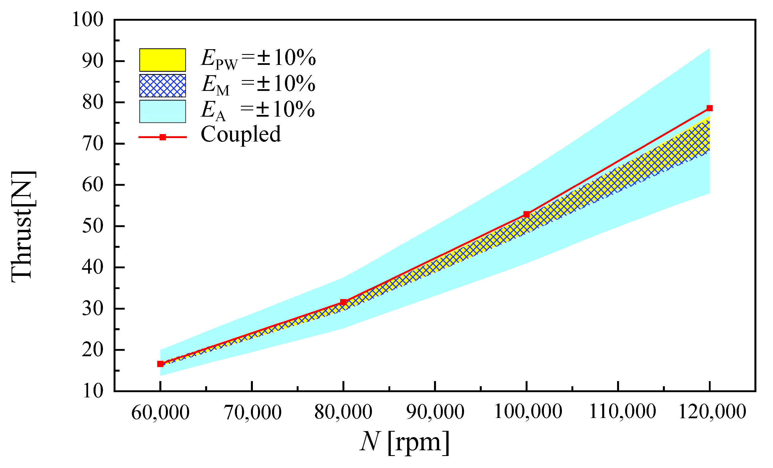
Second, the numerical error of the residual Equations (1)–(3) will also lead to inaccurate definite conditions for the 3D CFD simulation. Assuming an 10% error for $E_{\mathrm{M}}$, $E_{\mathrm{A}}$, $E_{\mathrm{PW}}$, the fuel supply and thrust characteristics of the engine are obtained based on ‘component-coupled’ simulation. The results are shown in Figure 9 and Figure 10. The color band reflects the range of the corresponding engine characteristic parameters under the specific error. The red line represents the calculation result of the ‘component-coupled’ simulation.

As shown in Figure 9 and Figure 10, the mass flow residual $E_{\mathrm{M}}$ and power residual $E_{\mathrm{PW}}$ have roughly the same effects on fuel consumption and the engine thrust especially at low rotation speeds. This reflects the positive correlation between power and mass flow. In fact, only when working at the choke state, this kind of positive correlation will no longer be valid. As for the throat area $\mathrm{A}$, it determines the expansion of gas in the nozzle and the static pressure at the outlet of the nozzle. As shown in Figure 10, the residual $E_{\mathrm{A}}$ had little impact on the fuel mass flow of the convergent nozzle, but had a more significant impact on the thrust. As we know, the convergent nozzle always works near the critical state. Compared with the mass flow, the static pressure at the outlet of the nozzle is more sensitive to the throat area $\mathrm{A}$. 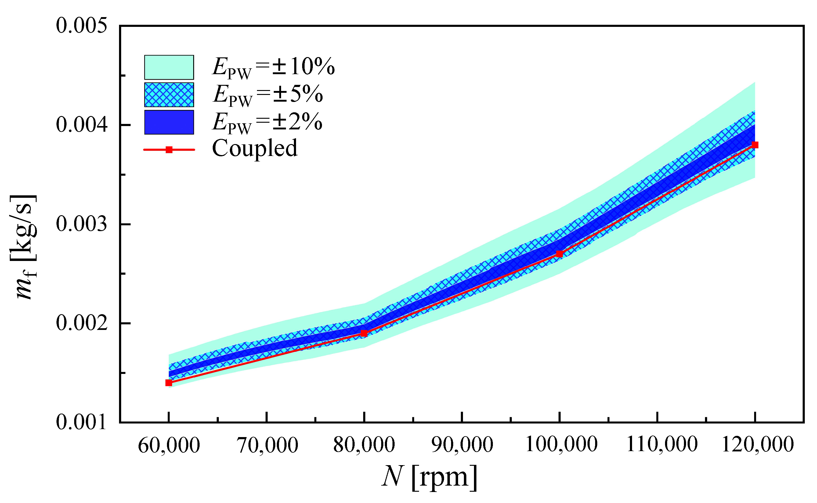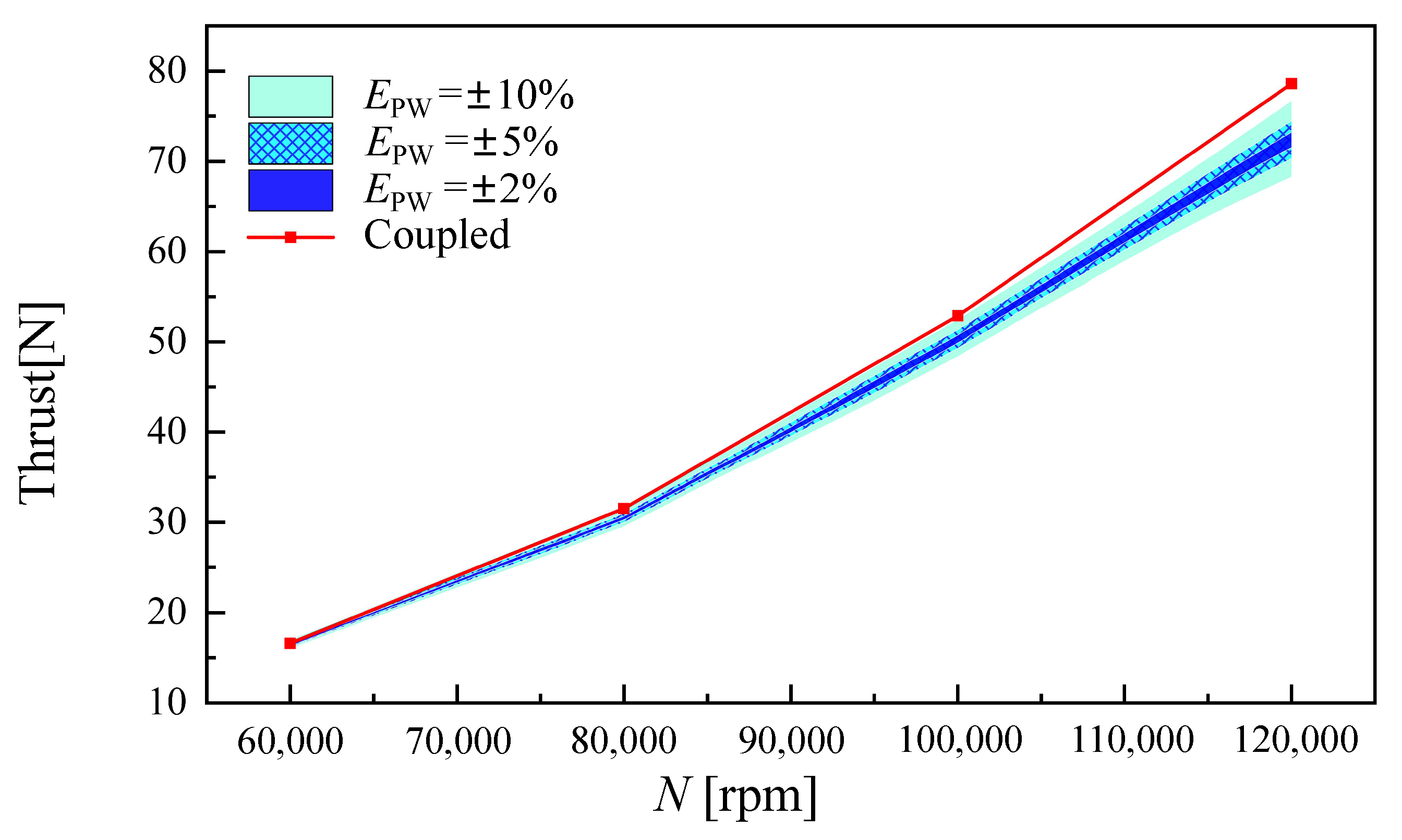For this reason, the throat area $\mathrm{A}$ directly affects the calculation of the pressure thrust. Taking the power residual as an example, the ‘component- matched’ simulations were carried out with $E_{\mathrm{PW}}=10\%$, $E_{\mathrm{PW}}=5\%$, and $E_{\mathrm{PW}}=2\%$, while ensuring that the errors of $E_{\mathrm{M}}$ and $E_{\mathrm{A}}$ were sufficiently small. As shown in Figure 11 and Figure 12, the color bands became finer as the power residual $E_{\mathrm{PW}}$ decreased. However, the ‘component-matched’ simulation results still deviate from the ‘component-coupled’ simulation results (the red line). This indicates that this deviation cannot be eliminated by improving the solving precision of residual equations.

Because of the difference in the models for ‘component-matched’ and ‘component-coupled’ simulation, the traditional practice of using the ‘component-matched’ simulation results as the input definite condition for ‘component-coupled’ simulation cannot avoid this kind of modelling error. Therefore, to overcome this defect in the current method, the power of the coaxial components must be matched automatically by introducing the power balance iteration into the steady-state 3D CFD solver.

3.2. The Influences of the Co-Working Constraints

The working state of the gas turbine engine can be represented by points in the parameter space. When working at steady state, these points can be regarded as the intersection points of the constraint surface $E_{\mathrm{M}}=0$, $E_{\mathrm{A}}=0$ and $E_{\mathrm{PW}}=0$. To analyse the effects of these co-working constraints on the engine state, the constraints were imposed one by one when solving the engine performance using the ‘component-matched’ simulation.

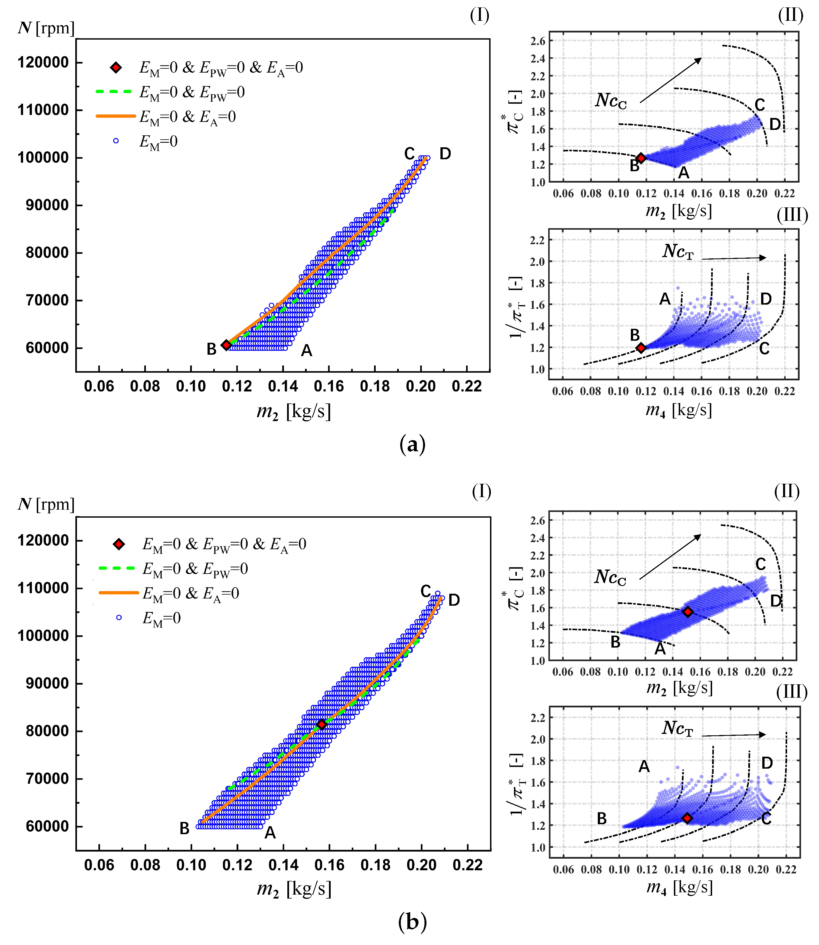
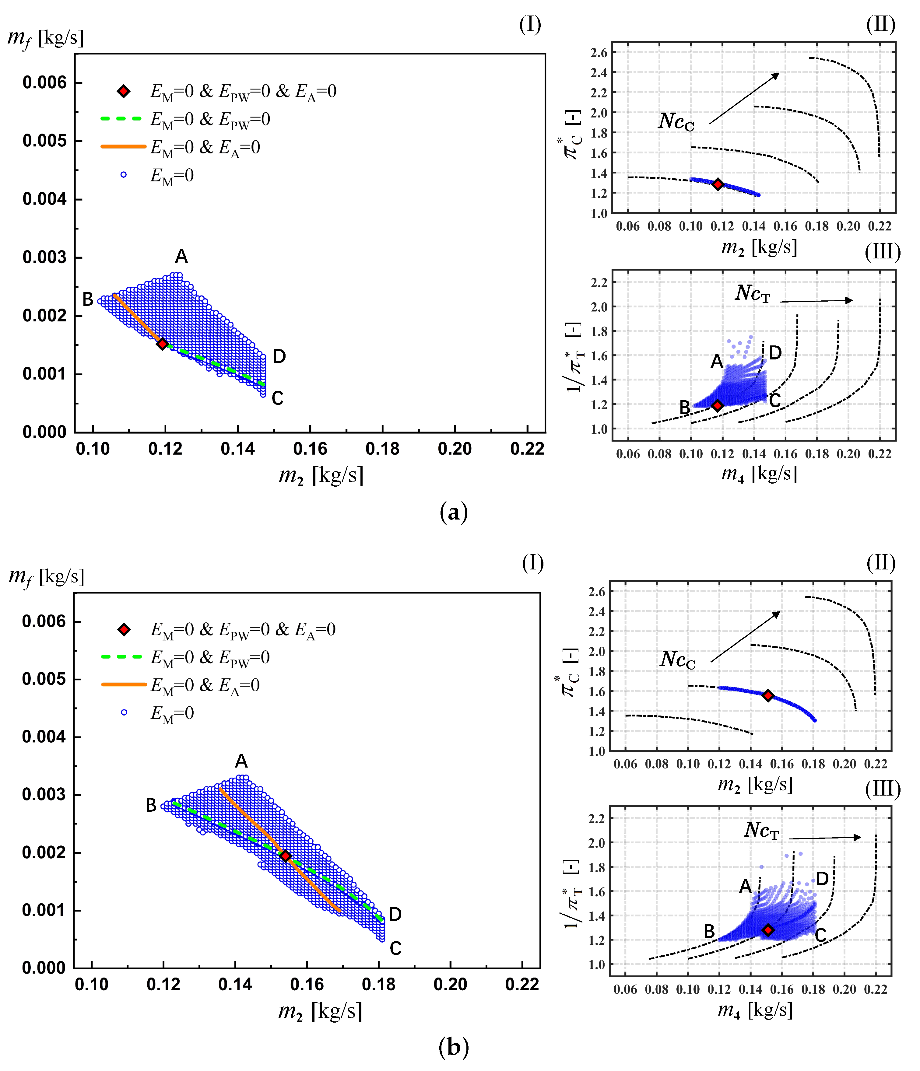
Taking rotation speed N as the iterative variable $X_i$, the feasible state points of the engine are constrained in the A-B-C-D zone by $E_{\mathrm{M}}=0$, as shown in Figure 13. The solid and dotted lines in Figure represent the feasible state of the engine when the mass flow constraint $E_{\mathrm{M}}=0$ and the throat area constraint $E_{\mathrm{A}}=0$ are added respectively. And the red diamond point represents the stable co-working state of the engine obtained with all constraints. The A-B boundary of the feasible region in Figure 13a,b is limited by the lowest speed line of the compressor characteristic map. The C-D boundary in Figure 13d is limited by the highest speed line of the compressor characteristic map. When the characteristic map is extended to lower and higher speeds, the feasible region in the parameter space will be the typical inverted-triangle shape similar to Figure 13c.

According to the characteristic maps, for the A-D boundary of the feasible region, the turbine works with the maximum corrected mass flow for a specific rotation speed. With the same mass flow, the physical rotation speed at the B-C boundary is larger than that at the A-D boundary. The compressor total pressure ratio is also higher. Considering the approximate isobaric combustion environment in the burner, the total turbine inlet pressure $P_4$ at the B-C boundary is higher, and the corrected mass flow $m{c}_4$ of the turbine is smaller than that at the A-D boundary. With a small change in the total pressure recovery coefficient of the burner, the B-C boundary of the feasible region is limited by the lower limit of the expansion ratio of the turbine. The expansion ratio of the turbine changes slowly and always tends to be $1.0$ at different rotation speeds, especially at a low corrected mass flow $m{c}_4$.

Taking fuel mass flow $m_{\mathrm{f}}$ as the iterative variable $X_i$, the feasible state points of the engine under different constraints are shown in Figure 14. Similar to Figure 13, the mass flow conservation constraint $E_{\mathrm{M}}=0$ limits the feasible state points to the area bounded by the A-B-C-D zone. In this region, the D-C boundary is limited by the maximum mass flow of the constant rotation speed line in the compressor’s map, just as shown in the Figure 14a,b. At the A-D boundary of the feasible region, the turbine works at the maximum corrected mass flow. At the BC boundary, the turbine works with a smaller expansion ratio at approximately 1.2. When the engine works at low rotation speed, the turbine is at the B-C boundary with a low mass flow. While at high rotation speed, the turbine approaches the choke boundary A-D. In contrast, the compressor is always in the peak efficiency area at different co-working points of the engine.

As shown in Figure 13 and Figure 14, regardless of whether the iterative variable is fuel mass flow or rotation speed, the stable co-working states solved by power balance iteration are almost the same. With the increase of fuel mass flow, the rotation speed also increases correspondingly. This positive correlation adheres to our intuition and is actually a general regularity for this kind of turbojet engine without many control parameters.

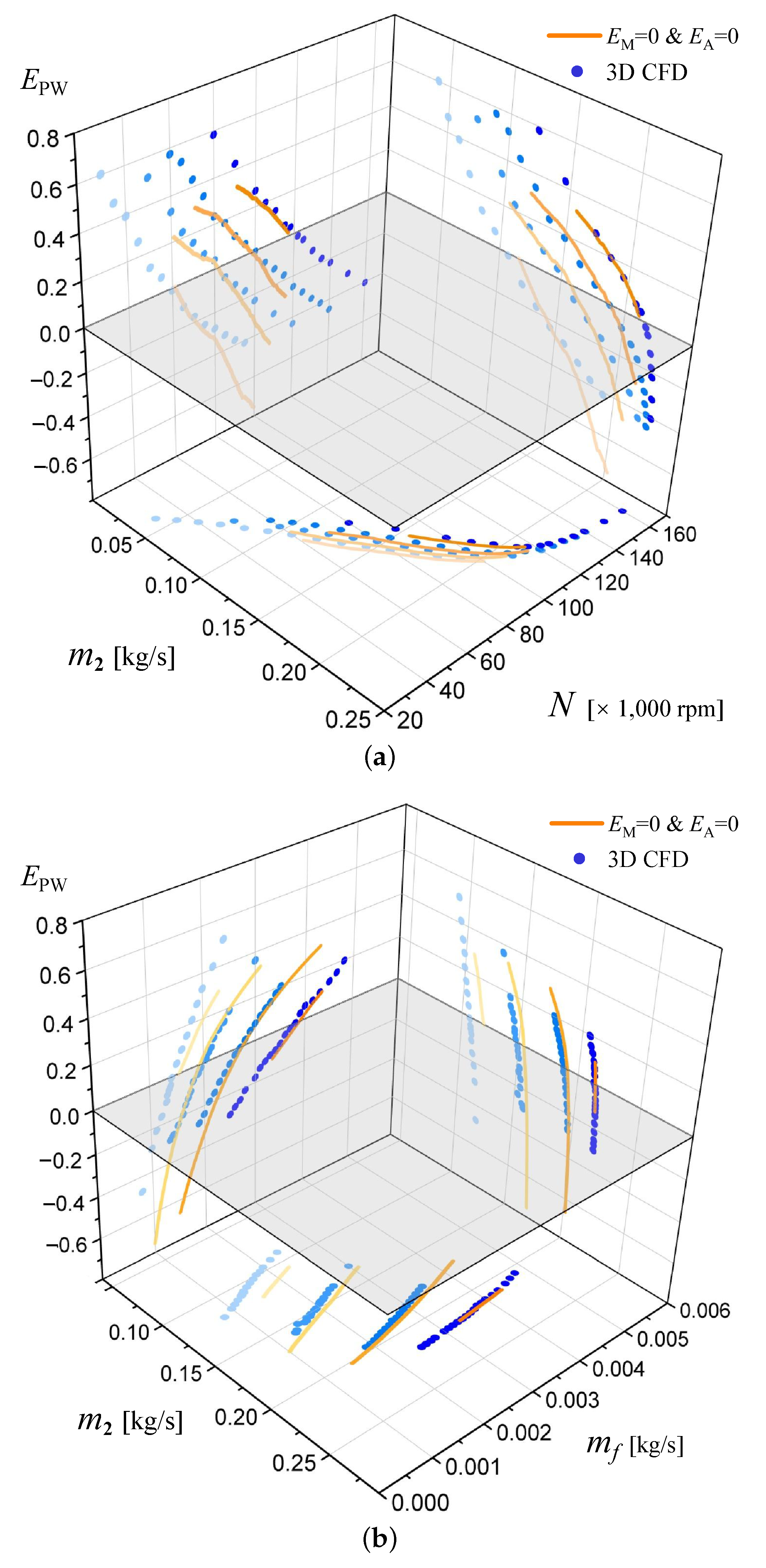
In addition, for the above 0D ‘component-matched’ simulation in Figure 13 and Figure 14, the state points with a release of power balance constraints fell onto the orange solid lines. The orange solid lines show the characteristics of local linearity. To verify this local linearity relationship, the ‘component-coupled’ 3D CFD method without power balance constraints was used to simulate these state points. The relationship between power residuals $E_{\mathrm{PW}}$, iterative variables $X_i$ and air mass flow of the engine $m_2$ are shown in Figure 15a,b for $X_i=N$ and $X_i=m_{\mathrm{f}}$ respectively.

The blue dots in the figures represent the calculation results of the 3D CFD simulation and the orange lines represent the 0D thermal simulation. Both of them are solved with the given rotation speed and fuel mass flow. In other words, the power balance constraints of the ‘component-coupled’ 3D CFD method and ‘component-matched’ 0D thermal method are both released to solve the results in Figure 15a,b. The orange lines in Figure 15 are correspond to the orange lines in Figure 13 and Figure 14.

As seen from Figure 15, the blue dots and the orange line have the same trend and basically coincide. This means in the steady 3D CFD calculation of the full engine, the co-working constraints $E_{\mathrm{M}}=0$ and $E_{\mathrm{A}}=0$ will be automatically satisfied when the aerodynamic parameters tend to be stable. However, the power balance constraints $E_{\mathrm{PW}}$ = 0 can be satisfied only at the specific fuel mass flow and rotation speed. This kind of state with only steady aerodynamic parameters but not with steady rotation speed can be regarded as a quasi-steady state.

More importantly, near the constraint plane $E_{\mathrm{PW}}=0$, the power residuals $E_{\mathrm{PW}}$ are inversely related to the rotation speed $X_i=N$, but proportional to the fuel mass flow $X_i=m_{\mathrm{f}}$. This means that when the turbine output power is greater than the compressor needs ($E_{\mathrm{PW}}>0$), the engine rotation speed N should be increased, or the fuel mass flow $m_{\mathrm{f}}$ should be reduced. If $E_{\mathrm{PW}}<0$, the engine rotation speed N should be reduced, or the fuel mass flow $m_{\mathrm{f}}$ should be increased.

The above analysis of the co-working constraints of the gas turbine engine is helpful to understand the key factors limiting the state of the engine and provides a basis for reasonable component matching design. This illustrates the weakness of the 0D thermal cycle ‘component-matched’ simulation. It highly depends on the component data models (general characteristic maps), which should be precise and complete. Taking the windmill state as an example, since the rotating parts are significantly affected by the incoming wind, the compressor and turbine may work in three states: ‘compressor state’, ‘turbine state’ and ‘stirrer state’. Therefore, a general characteristic map including the above three states must be provided to obtain the steady windmill state under the specific incoming flow. Moreover, because of the local linearity between the $E_{\mathrm{PW}}$ and $X_i$, the gradient ${(\partial E_{\mathrm{PW}}\left(X_i\right)/\partial X_i)}^k$ maintains the sign when solving the ‘component coupled’ 3D CFD simulation with power balance iteration according to the Formula (6). These characteristics can be used to develop the power balance iteration strategies in steady-state 3D CFD simulations.

3.3. Power Balance Strategies for Steady-State 3D CFD Simulation

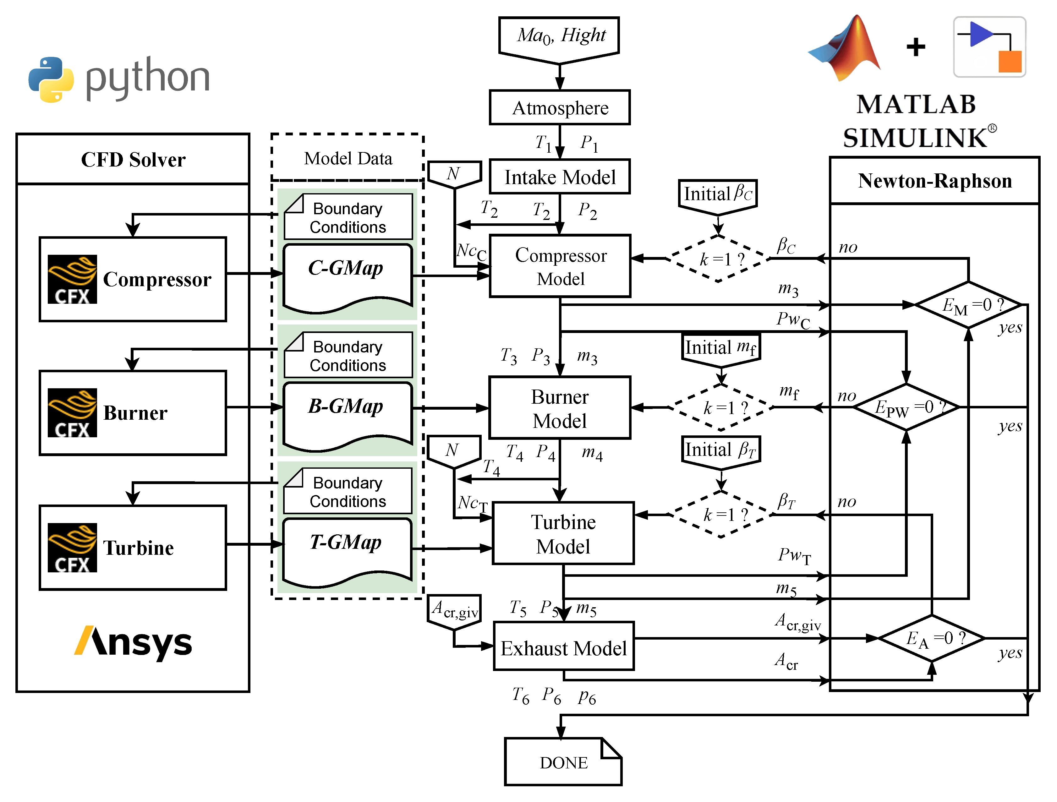
For the ‘component coupled’ 3D CFD method shown in Figure 2b, the parameters involved in the power balance iteration include the relaxation factor $\lambda$, the number of the timesteps per internal CFD calculation $n_{CFD}$ and the gradient $Gra{d}_{{\mathrm{E}}_{\mathrm{PW}}/{\mathrm{X}}_{\mathrm{i}}}$ = ${(\partial E_{\mathrm{PW}}\left(X_i\right)/\partial X_i)}^k$. The gradient $Gra{d}_{{\mathrm{E}}_{\mathrm{PW}}/{\mathrm{X}}_{\mathrm{i}}}$ can be estimated by the Regual-Falsi method and the power residual can be calculated using the flow field results of the previous internal CFD calculation. Therefore, whether the internal CFD calculation reaches a quasi-steady state is crucial for the accurate prediction of the gradient $Gra{d}_{{\mathrm{E}}_{\mathrm{PW}}/{\mathrm{X}}_{\mathrm{i}}}$ and affects the convergence of the power balance iteration. Unfortunately, numerical oscillation always exists even for the steady-state CFD calculations. Actually considering the calculation cost, the number of the timesteps $n_{CFD}$ for the internal CFD calculation should not be too large. Even if $n_{CFD}$ is large enough, the steady CFD calculation may still have large numerical oscillation due to the instability in calculating the combustion or the stalled compressor. This numerical oscillation makes it difficult to correctly estimate the size and sign (positive or negative) of gradient $Gra{d}_{{\mathrm{E}}_{\mathrm{PW}}/{\mathrm{X}}_{\mathrm{i}}}$.

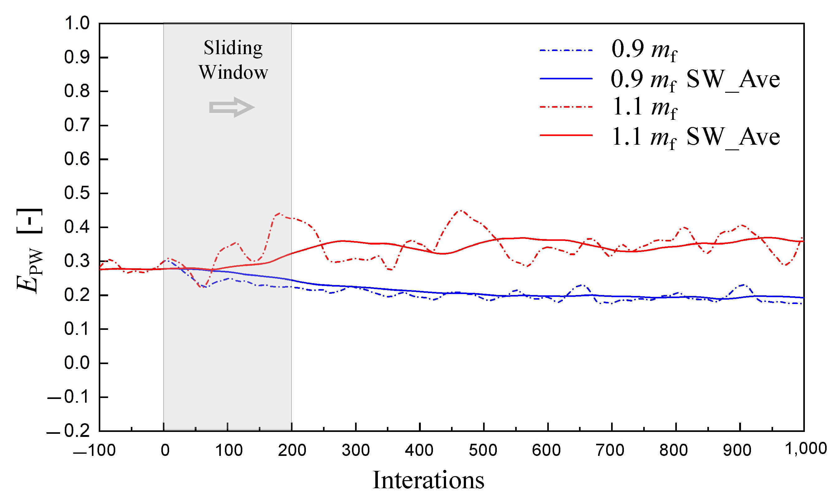
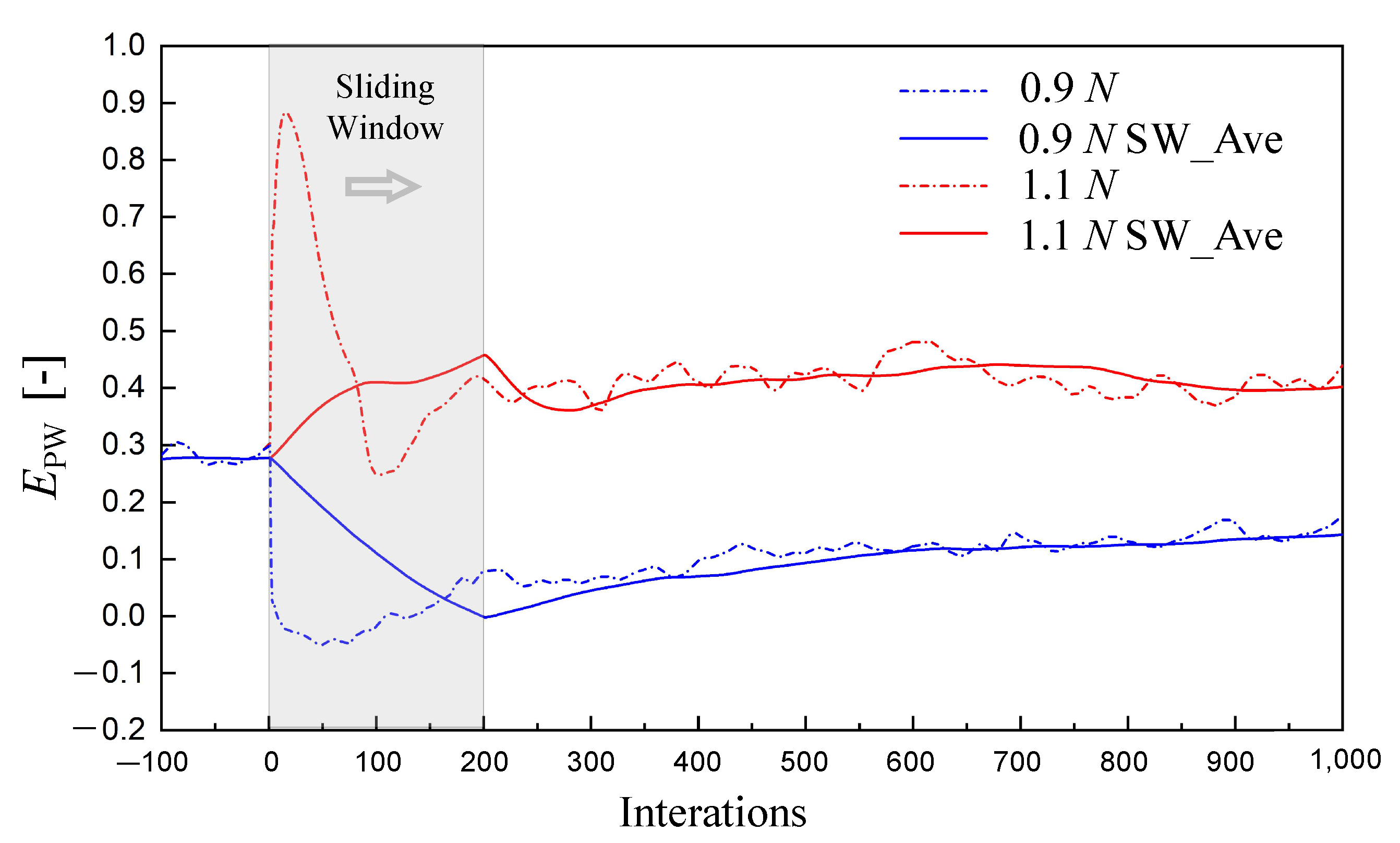
This numerical oscillation can be smoothed by averaging $E_{\mathrm{PW}}$ through a sliding window. Figure 16 and Figure 17 show the power residual $E_{\mathrm{PW}}$ obtained by CFD calculation with 10% forced perturbations of the $m_{\mathrm{f}}$ and N respectively. The initial field is a quasi-steady state with a rotation speed of 120,000 rpm and a fuel mass flow of 0.0035 kg/s. The dotted line is the calculation result of the steady CFD calculation, and the solid line is the result processed by the sliding window average (window width is 200). With sliding window treatment, the oscillation of the power residual is significantly reduced, which helps to reduce the numerical oscillation of the iterative gradient $Gra{d}_{{\mathrm{E}}_{\mathrm{PW}}/{\mathrm{X}}_{\mathrm{i}}}$ and stabilize the calculation.

Moreover, from the above figures, the oscillation of the power residual $E_{\mathrm{PW}}$ caused by changing the rotation speed N is significantly larger than that caused by changing the fuel mass flow $m_{\mathrm{f}}$ at the incipient stage. This means that the response of the power residual $E_{\mathrm{PW}}$ to the N is more sensitive than $m_{\mathrm{f}}$ in the numerical calculation process. Consistent with that shown in Figure 15, the change in air mass flow $m_2$ caused by changing rotation speed N is significantly larger than that caused by changing fuel mass flow $m_{\mathrm{f}}$. As we know, the change in rotation speed can affect the mass flow of the engine rapidly and has a greater impact on all components’ working state. Therefore, it is recommended to use fuel mass flow as the iteration variable $X_i=m_{\mathrm{f}}$ in the power balance iteration to make a numerical stability calculation.

Then, taking $X_i=m_{\mathrm{f}}$ as an example, a series of numerical tests were carried out to illustrate the effects of the relaxation factor $\lambda$, internal CFD time steps $n_{CFD}$ and gradient $Gra{d}_{{\mathrm{E}}_{\mathrm{PW}}/{\mathrm{X}}_{\mathrm{i}}}$ in power residual iteration. The parameter configurations for 6 sets of the numerical tests are shown in

Table 3. The parameter configurations of the ‘component coupled’ 3D CFD simulation with $X_i=m_{\mathrm{f}}$ and N = 120,000 rpm.

Case Name	${\mathit{n}}_{\mathbf{CFD}}$	$\mathit{\lambda }$	${\mathit{Grad}}_{{\mathbf{E}}_{\mathbf{PW}}/{\mathbf{X}}_{\mathbf{i}}}$
Case 1	300	$1.5$	Regual Falsi
Case 2	300	$0.5$	Regual Falsi
Case 3	300	$0.1$	Regual Falsi
Case 4	300	$1.5$	+200
Case 5	300	$1.5$	−200
Case 6	600	$1.5$	Regual Falsi

.

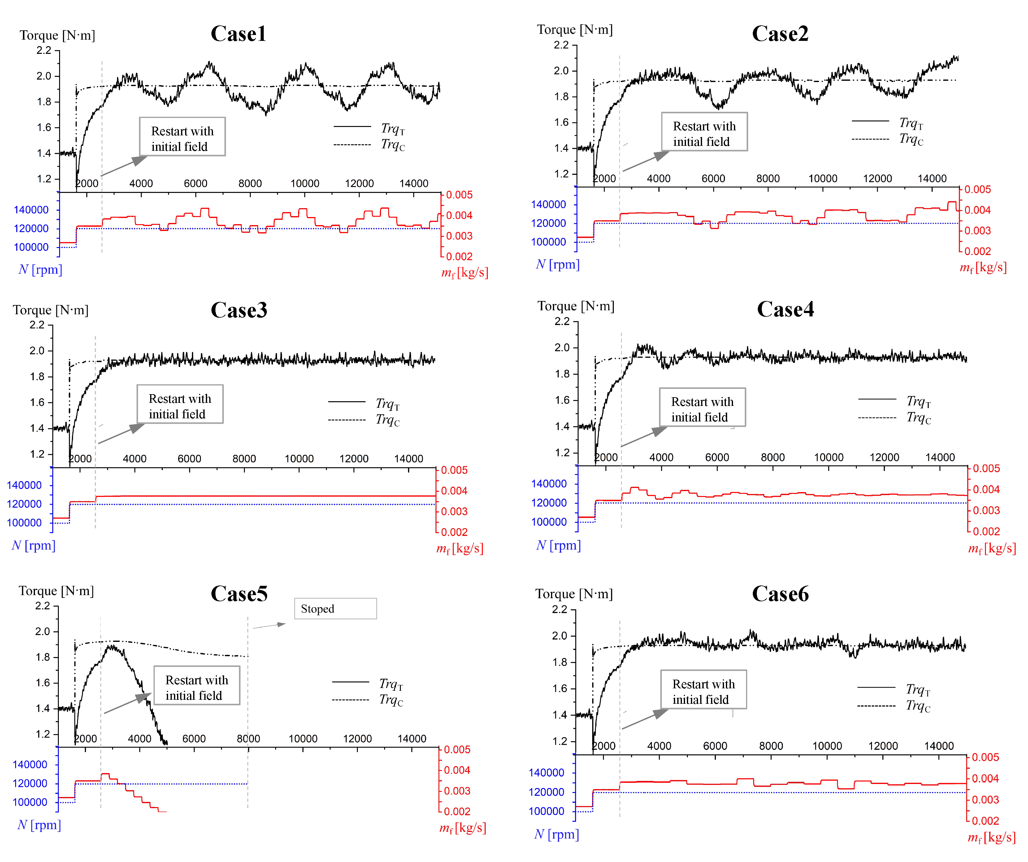
Figure 18 shows the iterative convergence history of power residual $E_{\mathrm{PW}}$ in these 6 tests. All the tests start from the same initial field and are expected to obtain the steady state of the engine at N = 120,000 rpm by automatically adjusting the fuel mass flow $m_{\mathrm{f}}$. The value of the gradient $Gra{d}_{{\mathrm{E}}_{\mathrm{PW}}/{\mathrm{X}}_{\mathrm{i}}}$ is given as a constant in Case 4 and Case 5. And for other cases, the gradient is calculated using the Regual Falsi method [33].

It can be seen that a large internal CFD time step $n_{CFD}$(e.g., Case 6) or a small relaxation factor $\lambda$ (e.g., Case 3) will be helpful for the convergence of power residual iteration. For Case 6, the number of the time steps $n_{CFD}$ is sufficient to make the aerodynamic parameters converge. And for Case 3, a smaller relaxation factor $\lambda$ means that the adjustment step of the iterative variables is small enough to reach a relatively steady state within a smaller number of steps $n_{CFD}$. For both of them, the convergence of power residual iteration is ensured. Considering the efficiency of the iterative calculation, $n_{CFD}$ should not be too large and $\lambda$ should not be too small. However, it makes the aerodynamic parameters calculated by internal CFD fluctuate wildly and then the power residual iteration may not converge, such as Case 1 and Case 2.

In addition, referring to the analysis conclusion in the Section 3.2, the gradients $Gra{d}_{{\mathrm{E}}_{\mathrm{PW}}/{\mathrm{X}}_{\mathrm{i}}}$ in Case 4 and Case 5 are set to be constant positive and constant negative respectively. The magnitude of the gradient is 200, which is the same as the magnitude reflected in Figure 15b. Given a positive gradient consistent with that in Figure 15b, the power balance iteration can converge stably (e.g., Case 4); however, when the gradient is negative, the iteration diverges very quickly (e.g., Case 5). 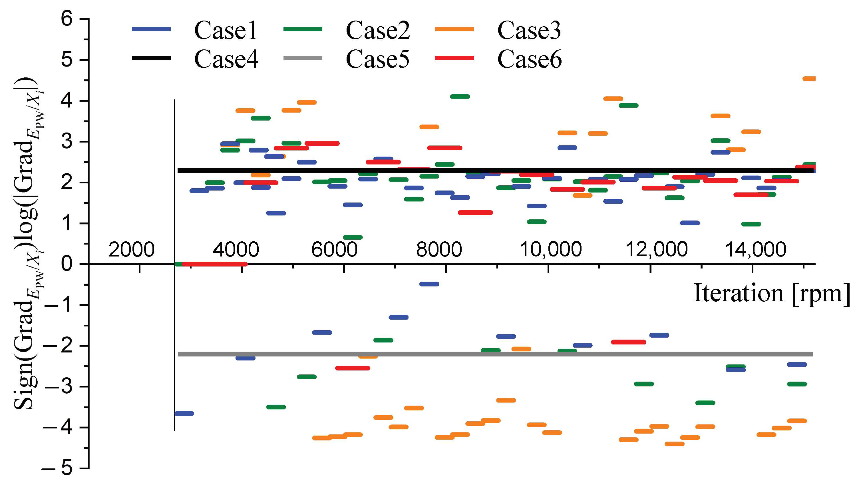The gradient $Gra{d}_{{\mathrm{E}}_{\mathrm{PW}}/{\mathrm{X}}_{\mathrm{i}}}$ is recorded during the power iteration for the above 6 simulation tests, as shown in Figure 19. Due to the fluctuations in the numerical calculation, the gradient $Gra{d}_{{\mathrm{E}}_{\mathrm{PW}}/{\mathrm{X}}_{\mathrm{i}}}$ parameter may vary over a large range. To observe the value clearly, the logarithm of the gradient $Gra{d}_{{\mathrm{E}}_{\mathrm{PW}}/{\mathrm{X}}_{\mathrm{i}}}$ is used as the ordinate in Figure 19.

When the gradient $Gra{d}_{{\mathrm{E}}_{\mathrm{PW}}/{\mathrm{X}}_{\mathrm{i}}}$ is basically positive, the power iteration can converge stably, such as Case 4 and Case 6. Otherwise, the power iteration diverges quickly, as in Case 5. When the gradient $Gra{d}_{{\mathrm{E}}_{\mathrm{PW}}/{\mathrm{X}}_{\mathrm{i}}}$ changes between positive and negative, the power iteration will be oscillated and did not converged, such as Case 1 and Case 2. It is worth noting that, with the smallest relaxation factor $\lambda$ in Case 3, the power iteration converges at $Interation\approx 5000$. Before this, the gradients $Gra{d}_{{\mathrm{E}}_{\mathrm{PW}}/{\mathrm{X}}_{\mathrm{i}}}$ calculated by the Regual Falsi method are all positive. After convergence, the gradient $Gra{d}_{{\mathrm{E}}_{\mathrm{PW}}/{\mathrm{X}}_{\mathrm{i}}}$ will oscillate between positive and negative with large amplitude. Actually, this oscillation is caused by the very small adjustment step of the iterative variable $X_i$, which is close to 0. As it is very small, the oscillation of the gradient will not cause the oscillation of the power balance iteration.

Although the aerodynamic parameters in the gas turbine engine are highly nonlinear, the characteristic parameters for typical steady states have certain local linear relationships. This is the reason why the gradient $Gra{d}_{{\mathrm{E}}_{\mathrm{PW}}/{\mathrm{X}}_{\mathrm{i}}}$ calculated by the Regual Falsi method can maintain its sign. In some extreme states, this local linear relationship may not exist. For example, if the fuel supply is greatly increased, the engine will work in an oil-rich combustion state. The combustion efficiency of the combustion chamber will be significantly reduced. Then the linear relationship between the power residual and the fuel mass flow will no longer exist.

Based on the above analysis, three strategies for power balance iteration are proposed:

Strategy I: Using the sliding window average to relieve the oscillation of the CFD simulation results, which improves the convergence of the external power balance iteration;

Strategy II: Considering the local linearity of the power residual and the iteration variable $X_i$, the signs of the gradient $Gra{d}_{{\mathrm{E}}_{\mathrm{PW}}/{\mathrm{X}}_{\mathrm{i}}}$ can be fixed, which can increase the stability of the iterative calculation;

Strategy III: It is recommended to take the fuel mass flow as the iteration variable $X_i=m_{\mathrm{f}}$, which will not lead to the drastic fluctuations of the engine state and make the calculation more stable.

4. Verification and Application

The micro-turbojet engines will stabilize at a specific rotation speed with different fuel mass flows. This correspondence can be described by the co-working line of the engine. The typical co-working states are simulated by the ‘component-coupled’ 3D CFD method to test its validity. The

Table 4. The relative error between simulation and experimental results.

N, rpm	60,000	80,000	100,000	120,000
$Er{r}_{\mathrm{Thrust}}$, %	−2.09	−2.72	−1.31	−4.10
$Er{r}_{\mathrm{SFC}}$, %	−13.22	−8.40	2.85	4.58

shows the relative errors of the results between the numerical simulation and experimental measurements at four typical rotation speeds. In Figure 20, the steady state thrust and specific fuel consumption (SFC) obtained by 3D CFD simulation are compared with the experimental measurement results in the reference [30]. The engine thrust parameters obtained by simulation are in good agreement with the experimental results. The trend of SFC is consistent with the experimental results. The error of the SFC is larger at low rotation speeds, but near the design state the accuracy is still claimed.

Similar to the steady-state co-working point, the power balance constraint condition may be satisfied after the engine is stabilized under an incoming wind. This wind-driven state of the engine, also known as the ‘windmill’ state, can be simulated using the ‘component-coupled’ 3D CFD method considering power balance iteration. For these states, the velocity of the incoming wind and the rotation speed of the engine should be matched to satisfy the power balance constraint.

For the micro-turbojet engine, it is usually started to the idling state using a blower or motor. At the blower-start state, the engine is in a stable ‘windmill’ state without fuel supply. The steady windmill characteristic line can describe these states. Figure 21 shows the steady-state co-working line and windmill line of the engine obtained by 3D CFD simulation. Herein, the digit number after the hyphen represents the rotation speed.

In the previous Figure 18, the convergence process of power balance iteration for the steady-state co-working state has been displayed. Figure 22 shows the convergence history of the torque and rotation speed in the simulation of the windmill states WmP-2 and WmP-4, which have approximately 20,000 $\mathrm{rpm}$ and 40,000 $\mathrm{rpm}$ rotation speeds. As the fuel is not supplied in these windmill states, the rotation speed can only be selected as the iteration variable during the power balance iteration, that is, $X_i=N$. The iterative parameters of power balance are set to $n_{CFD}=300$ and $\lambda =0.3$. As shown in Figure 22, the calculation result of WmP-2 was used as the initial field for the calculation of WmP-4. With no fuel supply, the steady states of the engine at a specific incoming flow are obtained by simulation.

According to the conclusions in the previous section, the change in rotation speed will directly affect the flow rate and have a great impact on the torque of the compressor and turbine. Therefore, the variation in torque caused by tuning the rotation speed will increase sharply in the power balance iteration, especially for solving the windmill state WmP-4, as shown in Figure 22. However, the internal CFD calculation cannot reach a quasi-steady state with $n_{CFD}=300$, and the flow field parameters are not stable. Through the adjustment of the iteration variable $X_i=N$, the power residual can eventually converge. The stability of the proposed method is presented. According to the simulation results, the main performance parameters of the engine at the final stable windmill state are shown in the

Table 5. The parameter of the windmill state WmP-2 and WmP-4.

	${\mathit{V}}_0$ [m/s]	$\mathit{N}\left[\mathbf{rpm}\right]$	${\mathit{m}}_2$ [kg/s]	${\mathit{\pi }}_{\mathbf{C}}^{*}$ [-]	${\mathit{\pi }}_{\mathbf{B}}^{*}$ [-]	${\mathit{\pi }}_{\mathbf{T}}^{*}$ [-]	$\mathbf{Trq}$ [N·m]
WmP-2	50	19275	0.0788	$0.979$	$0.959$	$0.968$	$0.0789$
WmP-4	86	39316	0.1755	$0.982$	$0.858$	$0.867$	$0.4022$

.

In Figure 23 and Figure 24, the key section of the burner and the meridional plane with circumferential mass weighted average parameter for other parts are generated to display the distributions of total pressure and total temperature. The co-working state CwP-4 and the windmill state WmP-4 with the same rotation speed of 40,000 $\mathrm{rpm}$ are both simulated. Not only can the state parameters of components be obtained for these two kinds of state, but detailed flow field information can also be provided.

As seen from Figure 23, constant pressure combustion occurs in the burner for these two states. Different from CwP-4, the total pressure at the inlet is significantly higher than the reference pressure for the windmill state WmP-4, and with a higher inlet velocity of 86 m/s. However, the centrifugal impeller also works on the incoming flow in the windmill state, resulting in an increase in the total pressure at the impeller outlet. The total pressure loss in the diffuser is obviously greater, which makes the total pressure ratio of the compressor less than 1. From Figure 23a, an obvious separation zone appears at the turning bend with the lower pressure on the hub side. In fact, as the velocity of the flow is larger in the windmill state, the passage and the blades of the diffuser cannot adapt to that flow condition and always have a high incidence. This is also the reason why the total pressure loss is obviously greater in the compressor diffuser under windmill conditions.

According to the figures, when the total pressure ratio of the compressor is less than 1 and the total temperature ratio greater than 1 under the windmill state WmP-4, the isentropic power of the compressor is negative and the actual power is positive. At this time, the compressor is under a so-called ‘stirrer state’ between ‘compressor state’ and ‘turbine state’. Actually, the centrifugal impelle is still under the ‘compressor state’ with a total pressure ratio and total temperature ratio greater than 1. This indicates that the work done by the impeller components on the air flow is not enough to compensate for the total pressure loss caused by the compressor, especially the diffuser. This is the main reason for the compressor to be in the ‘stirrer state’. For turbines, the turbine is driven by the high temperature gas at the CwP-4 state, while blown to rotate by the incoming wind at the WmP-4 state. For both states, the turbines are in the normal working state, the ‘turbine state’. From the 3D CFD simulation results, the turbine torque under the windmill state is $0.4022$ [N·m], while it is only $0.2081$ [N·m] for the steady state CwP-4 with the same rotation speed of 40,000 $\mathrm{rpm}$. As the power or torque is approximately proportional to the mass flow, the turbine power in the windmill state is larger than that in the state CwP-4.

From the analysis and verification above, the performances solved by this 3D CFD method for the KJ66 MTE are accurate within the allowable error range. Moreover, the ‘component-coupled’ 3D CFD simulation represents a great advantage not only for the calculation of the steady co-working state, but also for the windmill state, which is difficult to simulate by traditional methods. It can realize the calculation of engine performances and provide detailed data information of the full engine flow field.

5. Conclusions

In this study, the implementation process and technical route of the novel ‘component-coupled’ method with automatic power balance and the conventional ‘component-matched’ method are introduced. Taking the KJ66 Micro Turbojet Engine (MTE) as the research object, comparative studies of these two methods were carried out. The ‘component-coupled’ 3D CFD simulation method was implemented to simulate the steady state on the co-working line and the windmill line of the KJ66 MTE. The validity of this method is verified by comparison with the experimental results for the co-working state at the typical rotation speeds.

This article gets the following conclusions through the demonstration analysis:

(1) As the systematic error always exists, the traditional practice, inputting co-working state parameters as the definite conditions of the simulation, will lead to an obvious posterior error of the power balance. More importantly, when it is difficult to obtain the pre-given definite conditions, the usefulness of the full engine 3D CFD simulation would be severely limited. From this perspective, the necessity of introducing the power balance iteration to the solver is elucidated and the advantages and characteristics of the ‘component-coupled’ method with automatic power balance are revealed.

(2) The numerical oscillation of the CFD calculation has serious implications on the stability of the power balance iteration. For this reason, it is suggested to calculate the torque using the sliding window averaged CFD simulation results to relieve the oscillation (Strategy I). By recording the convergence history of the $E_{\mathrm{PW}}$ and the torque, the function of the sliding window average on the CFD results is illustrated.

(3) The influences of co-working constraints on the steady-state points of the engine were analysed by solving the feasible states with certain co-working constraint released. The results reveal the local linearity relationship of the power residual and the iterative variables. This explains why the signs of the gradient $Gra{d}_{{\mathrm{E}}_{\mathrm{PW}}/{\mathrm{X}}_{\mathrm{i}}}$ can be fixed in the iteration to stabilize the iteration (Strategy II).

(4) Both the fuel mass flow and the rotation speed can be taken as the iteration variable to realize the power balance. Changing the fuel mass flow cannot cause drastic fluctuations of the engine state and makes the iteration more stable. Therefore, the fuel mass flow is the first choice of the iteration variable for most cases (Strategy III). Exceptionally, for the windmill state with no fuel supplied, only the rotation speed can be taken as the iteration variable.

(5) This ‘component-coupled’ 3D CFD method seems to be a very promising approach for the windmill state, which is very difficult to simulate by the conventional component-based performance simulations. The simulation can also stably converge and the results can provide the detailed flow field for the windmill state. The ‘stirrer state’ of the compressor driven by the incoming flow was even captured by 3D CFD.

In this paper, only the power balance strategies for the steady simulation are discussed. The power matching method for the unsteady simulation is not involved. Actually, all the cases mentioned in this paper and in the references were carried out for the steady state of the gas turbine engine, whether based on the steady or unsteady CFD simulation. These power balance strategies can be used in steady simulations to provide a preferable initial field for the full engine unsteady CFD simulation. However, the capacity of this ‘component-coupled’ 3D CFD method with automatic power balance has been proven in this paper for a micro turbojet engine. For the other types of gas turbine engines, it is very worthwhile to explore the potential of the 3D CFD full engine simulation in further studies.