Article

Coverage Path Planning Method for Agricultural Spraying UAV in Arbitrary Polygon Area

1
College of Energy and Power Engineering, Nanjing University of Aeronautics and Astronautics, Nanjing 210016, China
2
College of Automation Engineering, Nanjing University of Aeronautics and Astronautics, Nanjing 211106, China
*
Author to whom correspondence should be addressed.
Aerospace 2023, 10(9), 755; https://doi.org/10.3390/aerospace10090755
Submission received: 26 June 2023 / Revised: 10 August 2023 / Accepted: 23 August 2023 / Published: 25 August 2023
(This article belongs to the Section Aeronautics)

Abstract

:
In the coverage path planning (CPP) problem of an agricultural spraying UAV, a margin reduction algorithm was designed first to address special situations such as ditches and channels within the operational terrain. Regarding the particularity of a concave polygon area, an algorithm based on topology mapping was developed to judge the concave points of the concave polygon area, and the path with special concave points was scheduled. For the evaluation of the pesticide spraying mission, the flight distance and extra coverage ratio were the most appropriate optimization objectives. Therefore, this paper selected these two indicators to form a fitness function, then found the optimal operating heading angle of the mission after iterative optimization. Finally, the CPP for an agricultural spraying UAV in an arbitrary polygon area under the optimal heading angle was realized. The simulation and flight test results showed that the CPP method could significantly shorten the flight distance and reduce additional coverage, then avoid energy consumption and pesticide waste. In addition, the engineering practicability of the method was verified in this paper. This method can be popularized and widely used for an agricultural spraying UAV, which has great engineering application value.

1. Introduction

The path planning of an UAV is to calculate the optimal or sub-optimal flight path according to the mission objective. At present, UAV path planning has in-depth research and technological development in the military and industry. The A* algorithm, genetic algorithm, and sparrow search algorithm have been widely applied in UAV path planning [1,2,3]. Yan, S. et al. researched the path planning problem of UAV multi-objective optimization [4,5,6] while Upadhyay, S. et al. proposed several practical obstacle avoidance methods in UAV path planning [7,8,9]. In addition, the application of multi-UAV cooperative operation mode is becoming more and more extensive. Savkin A. V. and Huang H. have made significant achievements in navigation and path planning for multi-UAVs and proposed an effective and optimal collision-free navigation algorithm. It is worth pointing out that the proposed method is not restricted to UAVs but also works for other types of mobile robots [10,11]. They also developed an MPC-based online method to plan the UAV’s 3D trajectory, promising to achieve better performance than optimizing the UAV’s trajectory [12]. Yao, P. et al. have made achievements in many research fields such as obstacle avoidance, minimum-time cooperative planning, mission allocation strategy, and so on [13,14,15]. For many sizeable agricultural production countries such as China and India, agricultural spraying UAVs have outstanding advantages in operating in paddy fields and between high stem crops, and performs well in explosive diseases or insect disasters. With the popularization of geographic information system (GIS) and global positioning system (GPS) technology and the development of sensor technology, autonomous agricultural spraying UAVs will become one of the essential fields in intelligent agriculture [16,17,18]. Studying the path planning method of agricultural spraying UAVs is necessary and meaningful [19]. For agricultural automation, the UAV must spray pesticides or perform other missions on a specific vegetation area. The path of the UAV needs to cover the whole area as much as possible. In other words, the path planning of an agricultural spraying UAV focuses on the CPP problem, which is to plan the optimal route to traverse the area to be covered under the premise of meeting the optimal mission indicators.
Agricultural spraying UAVs often adopt a cattle-plowing reciprocating operation mode [20,21], as shown in Figure 1. First, take a boundary in the area as the reference edge, then make a parallel line separated by half the spraying width. The distance between each parallel line is half the spraying width. The heavy line is the flight path of the agricultural spraying UAV, and the dotted line is the spraying boundary. Pesticide spraying will not be carried out in non-mission segments, and the arrow direction represents the operation direction of the UAV. However, pesticides will inevitably be sprayed outside the operating area. Moreover, the operating area of an agricultural spraying UAV is generally a convex or concave polygon area, rather than a simple or regular pattern such as rectangle, as shown in Figure 2.
Extensive research has been conducted on the CPP problem for a convex polygon area. Tan, G. proposed coverage path planning methods of the UAV operating area in a convex polygon, which is simple and universal [22]. Hong Y. proposed a comprehensive hardware and software architecture for autonomous area coverage missions using multiple UAVs in a convex polygon area and successfully conducted a flight test [23]. As for the CPP problem within a concave polygon area, researchers have often divided concave polygons into multiple convex polygons before conducting CPP. Choset, H. first proposed the boustrophedon cell decomposition method, which decomposed the complex operating area into simple basic areas [24]. Chen, H. proposed a CPP algorithm for UAVs in a convex polygon area and applied it to multi-UAV cooperative operation [25]. The concave polygon was cut into multiple convex polygons for path planning in the concave polygon area, so it was necessary to replan the path of the cut polygon according to the algorithm. Wang, Z. transformed the concave polygon area into a convex polygon area, then carried out a CPP that could cover the whole area [26], which is more suitable for multi-UAV cooperative operation. With the widespread application of UAVs in agricultural automation, there is an increasing focus on the efficiency of UAV task execution following a planned path. Shivgan, R. formulated the UAV path planning problem as a traveling salesman problem in order to optimize UAV energy, and proposed a genetic algorithm to solve the optimization problem to minimize the energy consumption for the UAV to complete a task [27]. Ahmadi, S. M. considered the scenario of monitoring a rectangular environment by a UAV to determine a path between the current position of the UAV and an arbitrary goal point that satisfied the handover time and smoothness constraints, then found the optimal path for the UAV to maximize the coverage of the designated area [28]. In the field of precision agriculture applications, Nolan, P. proposed a path planning method to generate vehicle trajectories aimed at tackling real-world data-sampling problems in the agricultural industry [29]. Mukhamediev, R. I. proposed a method of coverage path planning of a heterogenic UAV group, which provides flight planning by a group of UAVs using a moving ground platform on which the UAVs are recharged and refueled [30].
As the CPP of an agricultural spraying UAV lacks a general and systematic method that can be used in an arbitrary polygon area, and the flight distance and coverage ratio should be chosen as optimization objectives that are more suitable for pesticide spraying mission evaluation, this paper makes the following contributions. (1) We developed a general and efficient CPP method for an agricultural spraying UAV in an arbitrary polygon area. A margin reduction algorithm for the operating area was designed to aim at the particular situation such as the existence of ditches in the operating terrain. Especially for the concave polygon operating area, the area was divided into several sub-operating areas considering the influence of the concave angle and heading angle. (2) Achieving the CPP in irregular and over the entire operating area under the optimal heading angle reduces the mission’s complexity. Thus, we selected the flight distance and coverage ratio to form a fitness function and found the optimal operating heading angle of an agricultural spraying UAV after iterative optimization. (3) We adapted the devised algorithm into the flight controller to facilitate practical engineering implementation. Then, a flight test was carried out on farmland. The results verified the effectiveness of the algorithm, proving that the method proposed in this paper can be widely used in agricultural production activities.
The rest of this paper is organized as follows. Section 2 presents the CPP method for an agricultural spraying UAV in an arbitrary polygon area. In Section 3, the CPP method is incorporated into MATLAB to conduct simulations and we provide explanatory insights into the results. Section 4 encompasses the preparatory work and procedural implementation of the flight test. The outcomes validate the proposed method’s efficacy and engineering applicability. Finally, our work in this paper is concluded in Section 5.

2. Methodology for the Agricultural UAV CPP Problem

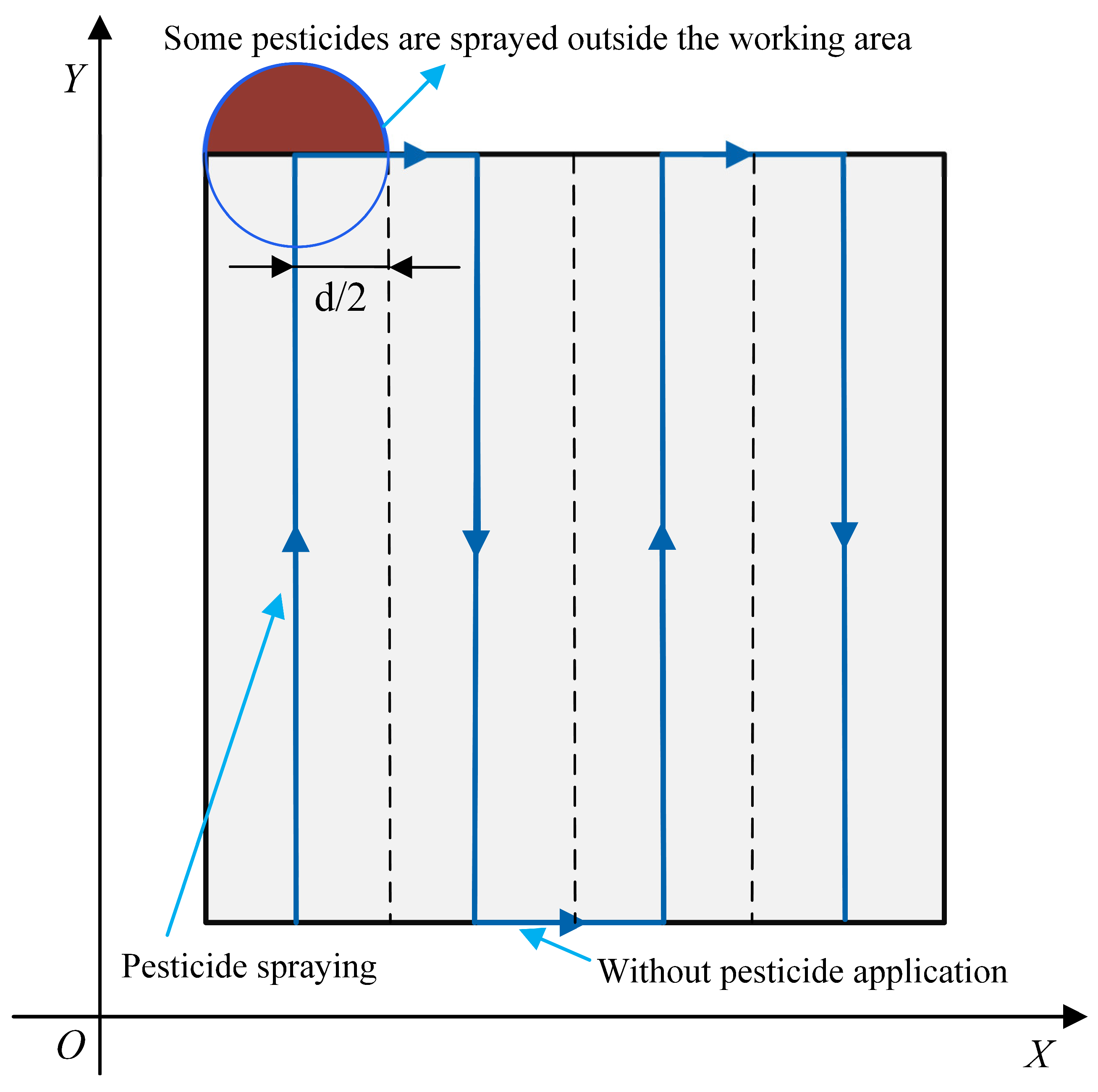
2.1. Margin Reduction of Operating Area for Agricultural Spraying UAV

Due to the particular operating form and operating area of agricultural spraying UAVs, users generally divide the operating area on the ground station map according to the boundary of the ditches. However, there is usually a gap between the ditch and the actual spraying area. If the boundary of the ditches is directly used as the operating area, it will lead to a waste of pesticides. Therefore, the margins of the operating area need to be reduced to avoid pesticide waste. According to the reduced margin value h input by users, shift every boundary of the operating area by a distance toward the interior of the graph. The distance is reduced margin value h .
As per the convex polygon operating area shown in Figure 3, number the coordinates of the polygon vertex in a clockwise direction ( D 1 D 2 D 3 D 4 D n , n means the number of vertices). D i is the corresponding vertex of D i after zooming out. D i D i must be parallel to and in the same direction as C according to a geometrical relationship. C is the normalized vector sum of two adjacent sides of the polygon:
C = D i D i 1 D i D i 1 + D i D i + 1 D i D i + 1
Then, obtain the corresponding interior angle θ of vertex D i according to Equation (2). Finally, we can work out coordinate D i according to Equation (3).
θ = a r c cos ( D i D i 1 D i D i 1 , D i D i + 1 D i D i + 1 )
D i D i = h sin ( θ 2 ) C C
We can obtain the coordinates of all the vertices of the new graph after transforming all of the vertices as above-mentioned. Reducing the margin of a concave polygon is similar to that of a convex polygon. The difference is that the concave point of a concave polygon has the opposite shift direction from the convex point compared with the margin zoom-out of a convex polygon. Therefore, we need to reverse the direction of vector D i D i formed by the concave point D i and its reduced corresponding point D i with C .
The new shape obtained after moving each boundary reduces the functionality compared to the original operating area. In this way, the flight distance of an agricultural spraying UAV is effectively shortened, the energy consumption is lowered, and the working efficiency is improved. The user can adjust h according to the terrain and plant direction appropriately after drawing an operating area. As a result, the influence of human factors on the final path quality during operating area planning is effectively eliminated. Meanwhile, the UAV still sprays pesticides when operating into the boundary of a new graph, which avoids pesticide waste, shortens the flight distance of the UAV, and improves the working efficiency.

2.2. CPP Algorithm in Convex Polygon Operating Area

For the selected convex polygon operating area, the area after margin reduction by the method above is D 1 D 2 D 3 D 4 D n , with n vertices and boundary lines. The equation of the boundary line is:
( y y D i ) ( x D i x D i 1 ) = ( x x D i ) ( y D i y D i 1 )
where x [ min ( x D i , x D i 1 ) , max ( x D i , x D i 1 ) ] . The number of flight routes r of the agricultural spraying UAV is calculated by ( y max y min ) / d , where y max and y min are the operating area’s maximum and minimum ordinate values, and d is the spraying width of the agricultural spraying UAV. Let multiple straight lines be parallel to the X-axis to intersect the operating area, the initial ordinate of the parallel straight lines is y min + d / 2 , and the distance between the parallel straight lines is the spraying width d . The intersection of the parallel straight line and the boundary of the operating area, which is the waypoint coordinates under the heading angle of 0 ° , can be solved by Equation (5):
y = y min + r i d / 2 ( y y D i ) ( x D i x D i 1 ) = ( x x D i ) ( y D i y D i 1 )
where x [ min ( x D i , x D i 1 ) , max ( x D i , x D i 1 ) ] . Number all operating routes from top to bottom. For odd-numbered routes, arrange waypoints from left to right; for even-numbered routes, arrange waypoints from right to left. All waypoints are organized according to this rule. Connect these waypoints sequentially to establish a comprehensive flight route for an agricultural spraying UAV with the heading angle of 0 ° . When the heading angle is ψ , divide the convex polygon work area into j triangles, where the centers of gravity are C 1 , C 2 C j , and the areas are A 1 , A 2 A j , respectively. Then, the center of gravity coordinate ( x t , y t ) of the convex polygon is solved by Equation (6):
x t = i = 1 j C i x A i i = 1 j A i , y t = i = 1 j C i y A i i = 1 j A i
Next, rotate convex polygon around ( x t , y t ) according to the heading angle ψ :
x = ( x D i x t ) cos ψ ( y D i y t ) sin ψ + x t y = ( x D i x t ) sin ψ + ( y D i y t ) cos ψ + y t
Let the new polygon obtained intersect with the line parallel to the X-axis to obtain the original waypoints. Then, rotate these waypoints in an anticlockwise direction due to the heading angle and connect them to obtain the desired flight route of the agricultural spraying UAV.

2.3. Concave Point Detection Based on Topological Mapping

The routes are continuous when the CPP is carried out in the convex polygonal area, but direct path planning in the concave polygon area such as the method in the convex polygon may cause too many routes to be outside the operating area. As a result, we needed to carry out necessary regional division and route scheduling, which will be detailed in the next part. Therefore, we must first effectively detect the concave point.
An algorithm based on topology mapping was utilized to determine the concavity and convexity of the polygon vertices. Following the tenets of topology mapping, we created a unit circle with a vertex of the polygon requiring evaluation at its center. Subsequently, we divided the unit circle into two semicircles, each of which corresponded topologically to two projective lines, denoted as L 1 and L 2 . In this way, the intersection of the unit circle and the vectors D i 1 D i , D i D i + 1 formed by two adjacent vertices of the vertex D i was also mapped on projective lines. Based on the different sides of the projection point on the projection line, it could be classified into four mapping situations, as shown in Figure 4. Under the premise of defining the arrangement order of polygon vertices (clockwise or anticlockwise), the intersection points of the unit circle and two adjacent edges of the vertex have topological invariance with their projective points on the projective lines since topology mapping is a unique and continuous correspondence relationship. Therefore, the position of the projective point on the projective lines can be used to judge the concavity and convexity of the vertex.
Assume that the arrangement order of the polygon vertices is anticlockwise. Set the coordinate value of vertex D i as ( x i , y i ) . The coordinate values of two adjacent vertices D i 1 , D i + 1 are ( x i 1 , y i 1 ) , ( x i + 1 , y i + 1 ) , respectively. Then, the two projective lines L 1 , L 2 are:
Y L 1 = y i + k Y L 2 = y i k
where k is a constant greater than 0, then the X-axis values of the two projective points on the projective lines are:
X X i 1 = ( x i x i 1 ) ( y y i ) ( y i y i 1 ) + x i X X i + 1 = ( x i + 1 x i ) ( y y i ) ( y i + 1 y i ) + x i
where y = Y L 1 or y = Y L 2 , in addition, y i y i 1 , y i y i + 1 . Assume k = 1 , then the difference of the coordinate value between the two projective points is:
δ = X X i 1 X X i + 1 = ( x i x i 1 ) ( y i + 1 y i ) ( x i + 1 x i ) ( y i y i 1 ) ( y i y i 1 ) ( y i + 1 y i )
We can judge which projective line the projective point is on through the Y-axis value of the vertex. The projective point is on projective line L 1 when y i > y i 1 , y i + 1 > y i . The projective point is on projective line L 2 when y i < y i 1 , y i + 1 < y i . Therefore, we can judge the concavity and convexity of vertices by analyzing the positive and negative of δ and ( y i y i 1 ) ( y i + 1 y i ) .
In the case of y i = y i 1 , set X X i 1 = + when x i > x i 1 ; set X X i 1 = when x i < x i 1 . Hence, the projective point can be categorized on either projective line L 1 or L 2 , akin to the situation y i = y i + 1 . Subsequent analysis mirrored the aforementioned approach and will not be reiterated.

2.4. CPP Algorithm in Concave Polygon Operating Area

As above-mentioned, the heading angle impacts the CPP in the concave polygon operating area with concave angles. Taking a certain concave angle, for example, draw a straight line parallel to the course and make the line pass through the concave angle. This straight line is called the reference line. The operating reference line will constitute two included angles together with adjacent two boundaries. If only one of these two included angles is the interior angle of the concave angle, the concave angle will be recorded as “Type 1”, and there will be no influence on the route due to the existence of this kind of concave angle. In case both the included angles are interior angles of the concave angle, the concave angle will be recorded as “Type 2”. As shown in Figure 5, where the UAV operates along the course from one side of the concave angle to the other side in the direction of the arrow, due to existence of the concave angle, it will not reach the working area at the other side if not crossing the non-operating area. As a result, the spraying route of the UAV is incoherent.
In order to ensure that each area can achieve the continuity of the spraying operating route and to avoid non-working routes as much as possible, we divided the concave polygon area into multiple sub-areas, where each sub-area’s path can be planned according to the method in the convex polygon operating area, then connects the completed route through the dispatch between the regions to obtain the final path. Only the influence of the “Type 2” concave point needs to be considered as the “Type 1” concave point does not influence the route. The division method is as follows: with the “Type 2” concave point as the starting point, draw a ray parallel to the flight route along the positive direction of the concave flight route, take the first intersection point of this ray with the graphic boundary, and connect with the vertex in sequence to constitute a sub-area. Repeat this operation for the n “Type 2” concave point to constitute n + 1 sub-areas. Figure 6a is the result of CPP under the given heading angle 0 ° in the concave polygon operating area. At this time, the concave point is “Type 2”, so route scheduling is required. Figure 6b shows the result of CPP under the given heading angle 90 ° , without the need for route scheduling.

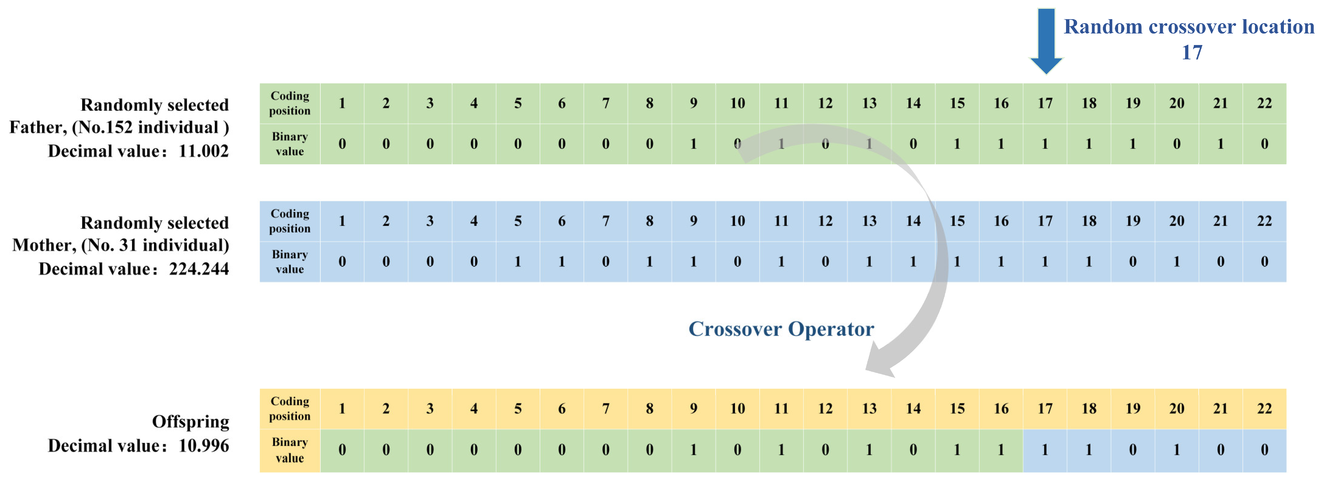
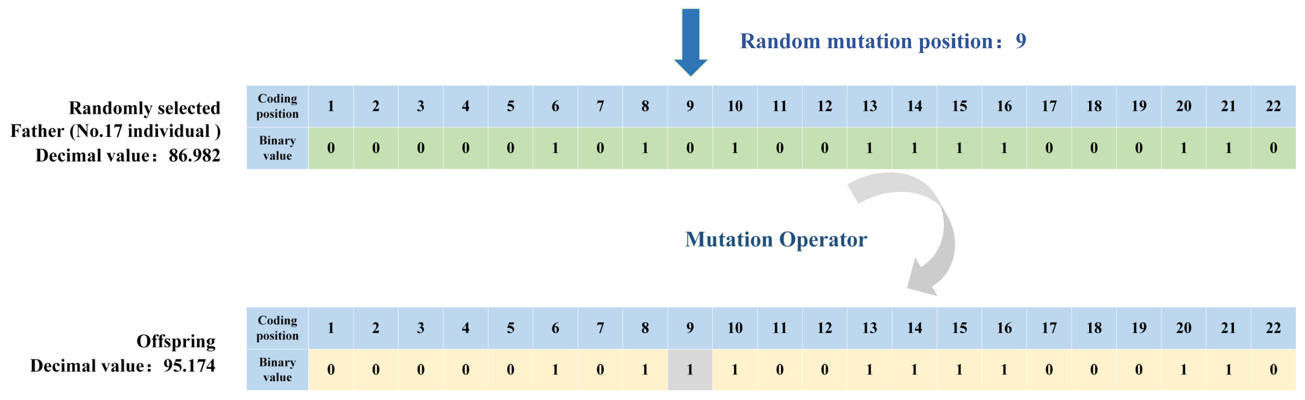
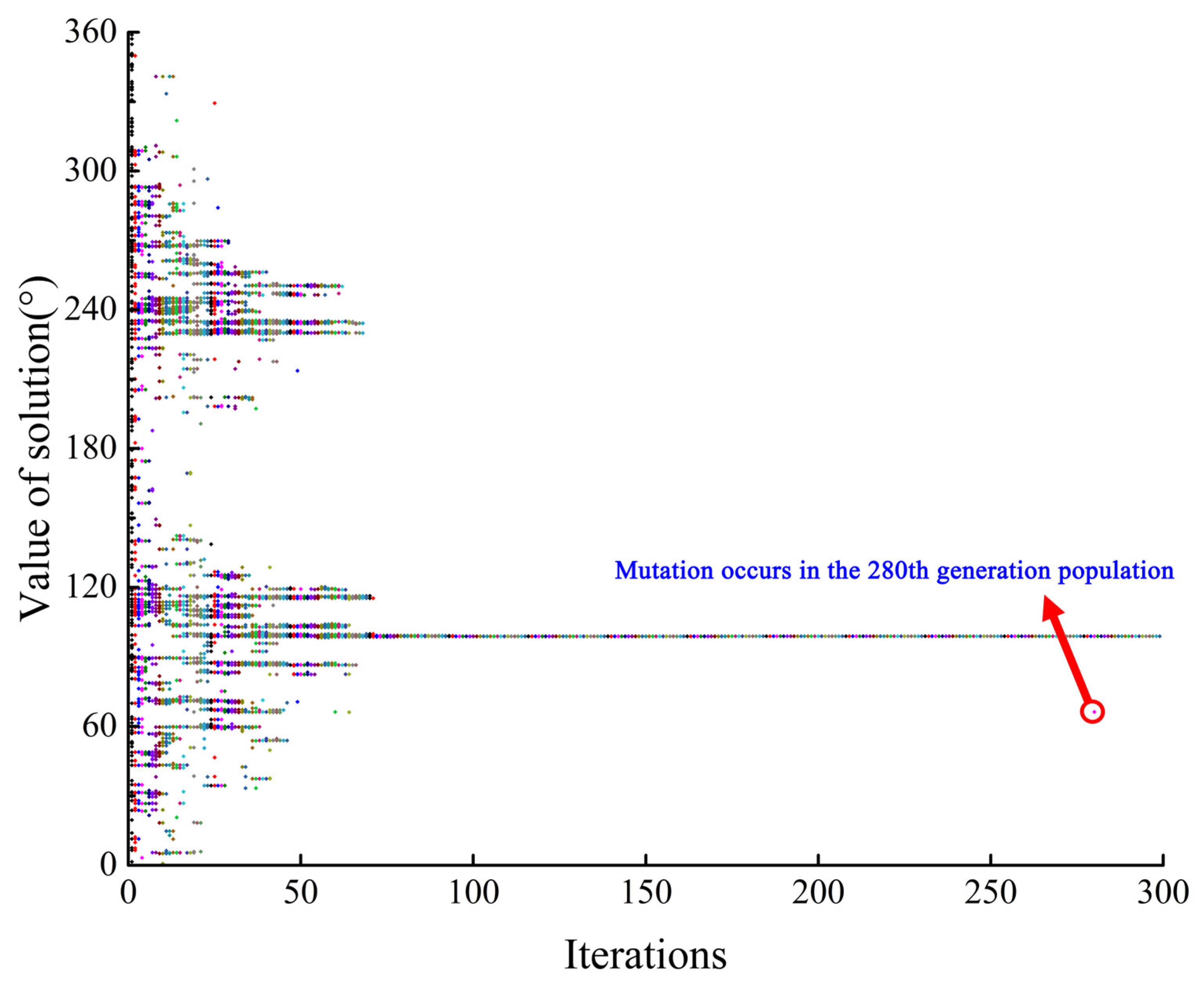
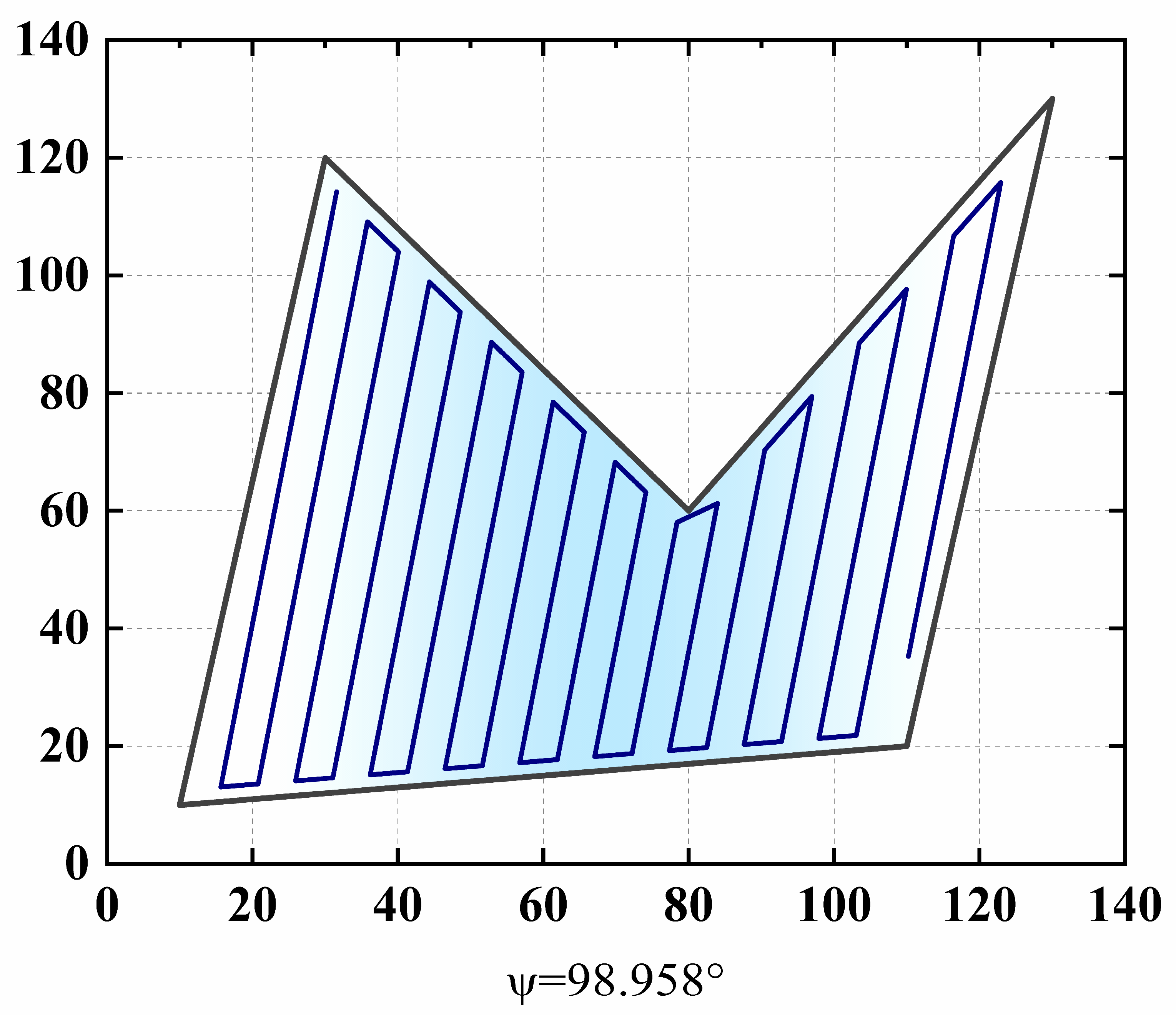
2.5. Heading Angle Optimization Based on Genetic Algorithm

In the previous section, it was introduced that route scheduling often occurs when the CPP is carried out in a concave polygon, which will cause agricultural UAVs to consume more power and waste more pesticides. Therefore, we need to find the optimal heading angle of CPP for an agricultural spraying UAV with flying distance and extra coverage ratio as the optimization objectives.
Addressing the challenge of the CPP problem concerning agricultural spraying UAVs, we randomly generated an initial population of 200 heading angles, each with a precision of three decimal places, spanning from 0 to 360 degrees. To create chromosomes, a 22-bit binary coding scheme is employed. The chromosome structure is represented by a digital string containing 0 s and 1 s, facilitating subsequent processes like crossover and mutation.
The selection of the fitness function directly affects the convergence speed of the genetic algorithm and whether the optimal solution can be found. The flight distance l and the extra coverage ε are selected as the indicators to establish the fitness function, where l 3000 m.
The flight distance of the agricultural spraying UAV can be calculated by accumulating the distances of each adjacent waypoint. Number the flight waypoints as p 1 , p 2 p n in the order of the route the UAV flew past. Then, in a single operating area, the flight distance can be calculated by Equation (11):
l = i = 1 n p 2 i p 2 i 1
The calculation equation of the extra coverage ratio is shown below:
ε = | i = 1 n p 2 i p 2 i 1 d S | S × 100 %
where p 2 i p 2 i 1 is the distance between two adjacent waypoints, d is the spraying width of the agricultural spraying UAV, and S is the operating area delimited by the user, then note the coverage area of the pesticide spraying:
S = i = 1 n p 2 i p 2 i 1 d
When S < S , it means coverage-omission; when S > S , it means coverage-repeat. Both of them need to be avoided. The smaller the extra coverage ε is, the smaller the area of spraying omission or repetition, and the better the operation effect.
The extra coverage ratio can be normalized, eliminating the area dimension. The extra coverage ratio can be selected as the component factor of the fitness function. Then, the flight distance generated by each generation of population should be normalized, and the normalization based on two-norm can be adopted:
l n o r m = l i / i = 1 α l i 2
Therefore, the fitness function selected above is:
f f i t n e s s = l n o r m + | i = 1 n p 2 i p 2 i 1 d S | / S 1
To avoid converging on the local optimum, the roulette wheel selection algorithm is used to iterate the population selection. In this method, the probability of an individual in the selected population is proportional to the value of the individual’s corresponding fitness function. We need to accumulate and normalize the fitness values of all individuals in the population and finally select the individual corresponding to the interval where the random number falls, which is similar to the rotating roulette in the casino. The algorithm adjusts the selection probability according to the adaptability of the genotype. In other words, a genotype can be selected multiple times, so the more adaptable genotypes to the environment have more chances of survival. First, according to the fitness of each individual f f i t n e s s ( a i ) , calculate the probability that each individual will be inherited into the next generation population:
P s e l e c t ( a i ) = f f i t n e s s ( a i ) j = 1 n f ( a j )
Then, calculate the cumulative probability of each individual:
Q s e l e c t ( a i ) = j = 1 i P ( a j )
After that, a random number r a n d is generated in the [ 0 , 1 ] . If r a n d < a 1 , then individual a 1 is selected to enter the next generation; otherwise, select individual a k , where a k 1 < r a n d < a k .
With the roulette wheel selection algorithm, the genotypes with low adaptability will be eliminated quickly, leaving only the genotypes with higher adaptability. Therefore, the genotype will tend to be single after several iterations, so the next step is to execute the crossover and mutation operations. The crossover operator plays a vital role in the genetic algorithm, which provides population chromosome variation and contributes to population evolution [31]. Figure 7 shows the crossover process of randomly selected individuals No. 152 and No. 31 in the second-generation population. Under the premise that the conditions for crossover operation are met, the crossover position on the chromosome is randomly generated, and the decimal value of the offspring generated by the crossover is 10.996.
The mutation operator replaces a gene with another gene on a chromosome with a certain probability. The mutation operator helps to impose diversity in the population and broaden the search space to avoid converging on the local optimum. Figure 8 shows the mutation process of the randomly selected individual No. 17 in the 29th generation population. The binary value at the ninth position randomly selected is reversed, and the decimal value of the offspring after mutation is 95.174.
The genetic algorithm concludes upon reaching the specified number of iterations, at which point the final generation’s population is updated to create the termination population. This termination population is expected to converge to a singular value. This value, represented in binary code, will then be decoded into a decimal representation, yielding the optimal heading angle.
The algorithm process is outlined in the following Algorithm 1. Once the complete algorithm is implemented in MATLAB, a digital simulation can be conducted to validate its accuracy.
Algorithm 1: CPP algorithm for agricultural spraying UAV in the arbitrary polygon area based on genetic algorithm.
Aerospace 10 00755 i001

3. Implementation of Algorithm, Simulation, and Data Analysis

We incorporated the CPP algorithm for heading angle optimization into MATLAB to conduct the simulations [32]. Initially, the operational area’s margins were adjusted to account for the crop growth patterns and pesticide spraying requisites. An initial population of heading angles was generated randomly, and these angles were encoded for iterative optimization. Within the area, concave points were identified, and subsequently, the flight distance and surplus coverage were computed to derive the fitness function value. This value was then utilized to execute crossover and mutation operations, culminating in determining the optimal heading angle through a genetic algorithm approach. Notably, CPP within the concave polygons involved intricate sub-regional division and route scheduling, presenting greater complexity compared to convex polygons. Consequently, the simulation results for CPP in concave polygons were analyzed in this section. The CPP procedure was executed within the operational area using the optimal heading angle. The initialization parameters for the algorithm are presented in Table 1.
The depiction of the fitness function values for each individual within every generation of the population is illustrated in Figure 9. Initially, the value of each fitness function differed significantly. With the selection of each iteration, the distribution of the fitness function value gradually tended to concentrate, and finally converged to the same value.
The mean value and the standard deviation of the fitness function per generation population is shown in Figure 10. In the initial population, the fitness function value of individual No. 153 with the largest fitness value was 5.0532, and the fitness function value of individual No. 27 with the smallest fitness value was 1.9130. The standard deviation of the fitness value of the initial population was the largest, and its value was 0.8685. It can be seen that the mean value almost approached the maximum value after about 71 iterations, and the standard deviation was 0.043. Finally, the fitness function attained its peak value of 5.0864, accompanied by a standard deviation of 0 after 173 iterations.
The distribution of all individuals in each generation of the population is shown in Figure 11. Its convergence trend was consistent with the convergence trend of the fitness value above-mentioned, and it gradually stabilized after 71 iterations. After gradually stabilizing, another mutation occurred in the 280th generation population, but the offspring population obtained by the mutation had a smaller fitness value. Then, the mutant individual and its offspring were soon eliminated. Finally, after 300 iterations, the population convergence was terminated, and all individuals were 98.958, so the optimal heading angle of 98.958 ° for the operating area was obtained.
Under the optimal heading angle of 98.958 ° , the waypoints can be calculated to generate the flight path. Figure 12 shows the result of CPP under the optimal heading angle.
.
In order to reflect the best mission effect of an agricultural spraying UAV, we took the fitness function value rather than the flight distance or extra coverage ratio as the criterion. When the population finally converged, the fitness function value reached the maximum, and the flight distance and extra coverage ratio of the agricultural spraying UAV should converge to a smaller value accordingly. Figure 13 shows the relationship between the mean flight distance of each generation and the mean fitness function value in the process of population convergence. It can be seen from Figure 13 that when the flight distance is smaller, the corresponding fitness function value is larger. As the number of iterations increases, the maximum fitness function value is reached when the solution value converges to the optimal heading angle of 98.958 ° , and the corresponding flight distance is 1439.6 m.
The relationship between the mean extra coverage ratio of each generation and the mean fitness function value in the population convergence is shown in Figure 14. It can be seen that the corresponding fitness function value was larger when the extra coverage ratio was smaller. As the number of iterations increased, the solution value converged to the optimal heading angle, and the extra coverage ratio was 12.59%. In other words, the CPP was carried out under the optimal heading angle of 98.958 ° in the selected concave polygon operation area. The flying distance was 1439.6 m, and the extra coverage ratio was 12.59%.

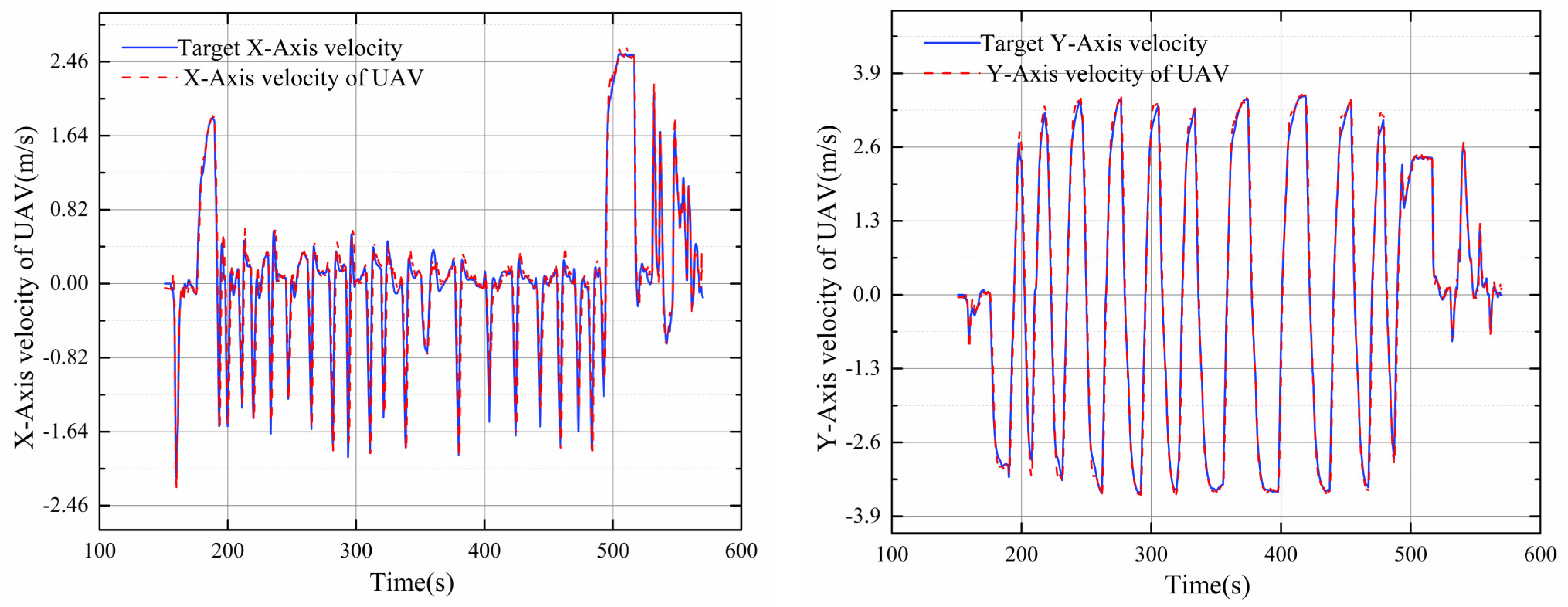
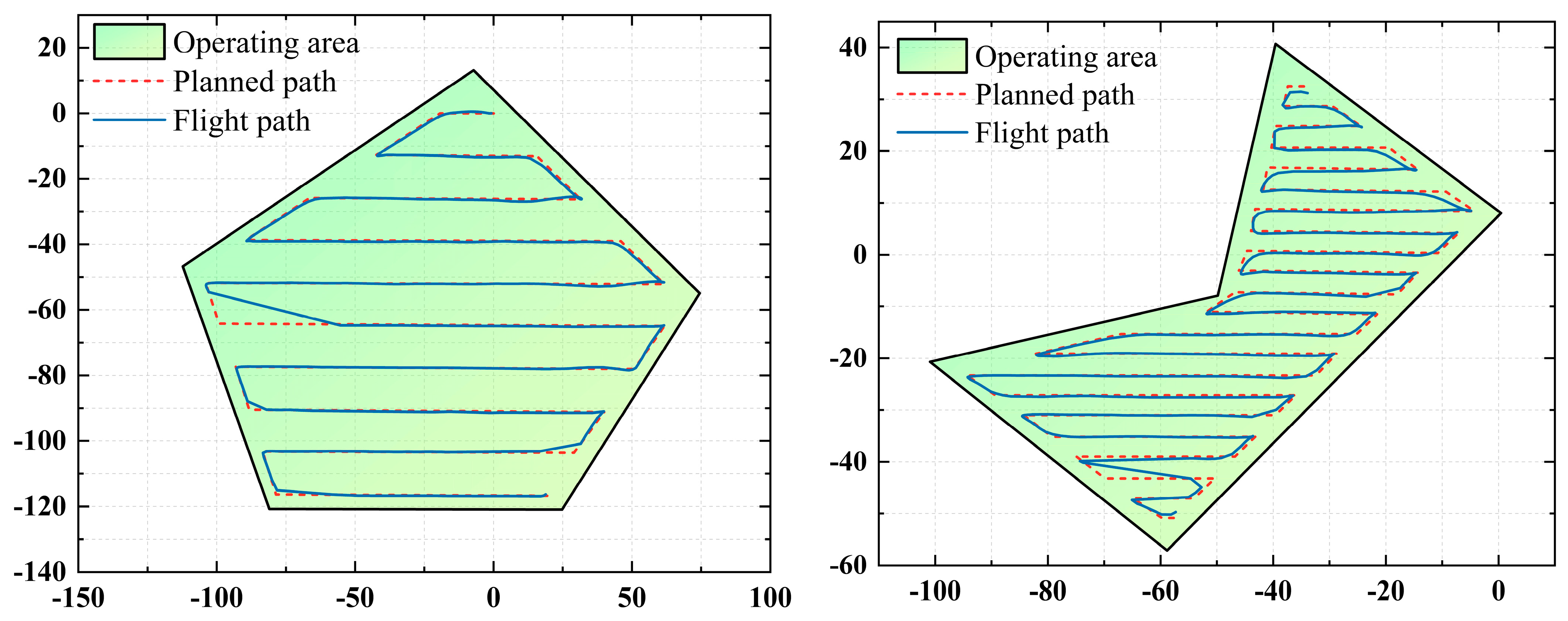
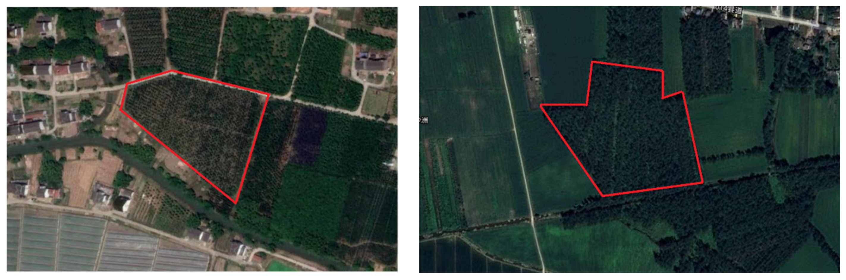
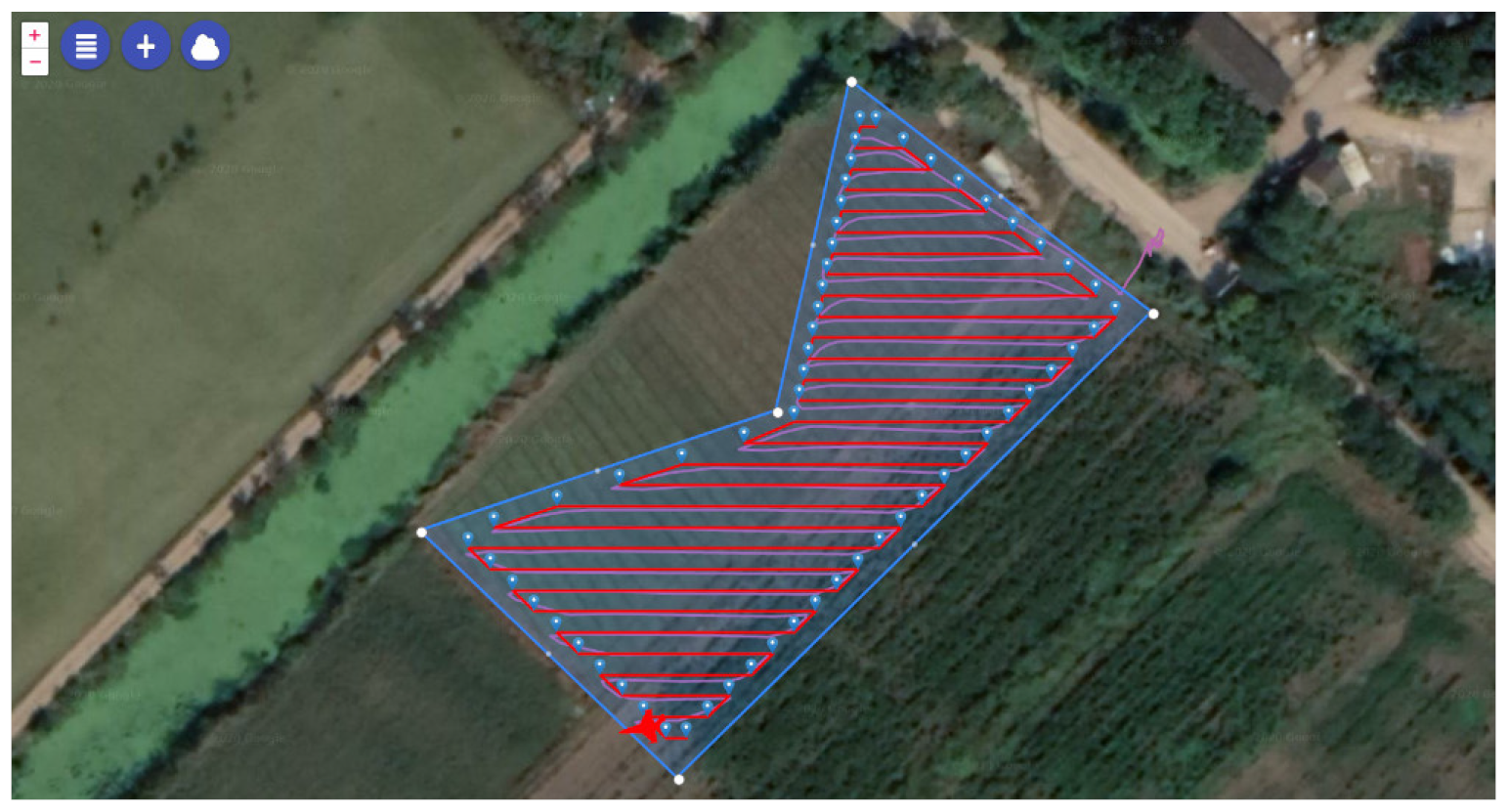
4. Engineering Application and Flight Test

In the preceding section, the accuracy of the algorithm was verified by a MATLAB simulation. In this part, we applied the algorithm to the ground control station, which was developed in the QT environment to generate the operating route of an agricultural spraying UAV [33]. Subsequently, flight tests were conducted within farmland environments to ascertain the algorithm’s practical viability in engineering applications. For this purpose, a specific farmland was chosen as the experimental site. The agricultural spraying UAV employed for the flight tests and the operational setting are illustrated in Figure 15.
We carried out the CPP under the optimal heading angle in the convex and concave polygons, as shown in Figure 16 and Figure 17, respectively. First, the user selects the boundary points of the target operating area (i.e., the white points in the figure) on the map of the ground control station. Then, the station will automatically generate the operating area shown in the blue line in the figure. At this time, the ground control station has converted the longitude and latitude of the operating area into two-dimensional coordinates. The red line in the figure is the best path planned by the station according to the parameters designated by the user; the purple line is the actual flight path of the UAV. In addition, the ground control station also shows the operating time, operating area, flight distance, extra coverage ratio, and other information.
We recorded the flight experiment log of the flight mission. For the path planning mission corresponding to the operation area in Figure 17, the pitch angle, roll angle, yaw angle, and their desired values for the UAV are shown in Figure 18, Figure 19 and Figure 20. It can be seen from the figures that the attitude of the agricultural spraying UAV changed regularly with the path direction.
In addition, we also recorded the displacement and velocity data in the X and Y directions of the UAV. The results are shown in Figure 21. It can be seen that the displacement response of the agricultural spraying UAV in the X-axis and Y-axis is consistent with the planned path, and the actual flight path could follow the planned path well.
The velocity response is shown in Figure 22. The velocity response of the agricultural spraying UAV in the X-axis and Y-axis reflects the state of the agricultural spraying mission well.
The operating area, planned path, and actual flight path of the UAV are depicted in Figure 23. The green area is the selected working area, the red dotted line is the flight path under the optimum heading angle generated according to the method in this paper, and the blue solid line is the actual flight path of the UAV. It can be seen that the UAV could navigate well according to the planned path. In Figure 23, the fact that the UAV does not sometimes fly according to the planned path is caused by the loss in the data transmission radio signal, resulting in the loss of information of several waypoints in the middle, then the recorded flight log directly connects the two final recorded waypoints into a line segment. A slight deviation between the actual path and the theoretical path in the flight test was caused by the GPS positioning error of the UAV and other environmental factors such as airflow. Overall, the flight test was successful, and the agricultural spraying UAV could track the theoretical flight path well, which verifies the engineering practicability of the CPP method in this paper.

5. Conclusions

This paper proposed a general and easy-to-implement CPP method. The objective for agricultural spraying UAV operations is to enhance endurance and optimize pesticide consumption while accomplishing spraying tasks. Different path directions yield different waypoints, flight distances, and extra coverage. Thus, the essence of this method involves determining the optimal heading angle, forming the basis to calculate the final waypoints. Significantly, in the context of concave polygon operating areas, the region is subdivided into several sub-operating zones, considering the impact of both concave angles and heading directions. This division facilitates CPP within irregular and expansive operational domains under the optimal heading angle, thereby simplifying mission intricacies. Moreover, the algorithm was integrated into the flight controller to enable practical engineering applications. Subsequent flight tests conducted within farmland environments demonstrate the ability of the agricultural spraying UAV to execute pesticide spraying missions in accordance with the planned path. These outcomes validate the algorithm’s efficacy. Consequently, the CPP method proposed in this paper can be broadly applied to agricultural production activities.

Author Contributions

Conceptualization, H.S.; Methodology, J.L.; Validation, J.L.; Formal analysis, J.L.; Investigation, J.Z.; Data curation, H.S.; Writing—Original draft preparation, J.L.; Writing—Review and editing, J.Z.; Supervision, H.Z. All authors have read and agreed to the published version of the manuscript.

Funding

This research was supported by Funding of National Key Laboratory of Rotorcraft Aeromechanics (No. 61422202108).

Data Availability Statement

The data presented in this study are available on request from the corresponding author.

Conflicts of Interest

The authors declare no conflict of interest. The funders had no role in the design of the study; in the collection, analyses, or interpretation of data; in the writing of the manuscript; or in the decision to publish the results.

References

  1. Xu, W.; Zhang, Q.; Zou, Y.; Zhang, H.; Chen, Y. Research on Transportation Path Planning for Logistics UAV Based on Improved A* Algorithm. J. East China Jiaotong Univ. 2019, 36, 39–46. [Google Scholar] [CrossRef]
  2. Liu, H. A Novel Path Planning Method for Aerial UAV based on Improved Genetic Algorithm. In Proceedings of the 2023 Third International Conference on Artificial Intelligence and Smart Energy (ICAIS), Coimbatore, India, 2–4 February 2023; pp. 1126–1130. [Google Scholar] [CrossRef]
  3. Liu, G.; Shu, C.; Liang, Z.; Peng, B.; Cheng, L. A modified sparrow search algorithm with application in 3D route planning for UAV. Sensors 2021, 21, 1224. [Google Scholar] [CrossRef] [PubMed]
  4. Yan, S.; Cai, K. A multi-objective multi-memetic algorithm for network-wide conflict-free 4D flight trajectories planning. Chin. J. Aeronaut. 2017, 30, 1161–1173. [Google Scholar] [CrossRef]
  5. Cowlagi, R.V.; Sperry, J.P.; Griffin, J.C. Unmanned aerial vehicle trajectory optimization for executing intelligent tasks. J. Guid. Control Dyn. 2018, 41, 1389–1396. [Google Scholar] [CrossRef]
  6. Xu, L.; Cao, X.; Du, W.; Li, Y. Cooperative path planning optimization for multiple UAVs with communication constraints. Knowl. Based Syst. 2023, 260, 110164. [Google Scholar] [CrossRef]
  7. Upadhyay, S.; Ratnoo, A. Smooth path planning for unmanned aerial vehicles with airspace restrictions. J. Guid. Control Dyn. 2017, 40, 1596–1612. [Google Scholar] [CrossRef]
  8. Pham, T.H.; Bestaoui, Y.; Mammar, S. Aerial robot coverage path planning approach with concave obstacles in precision agriculture. In Proceedings of the 2017 Workshop on Research, Education and Development of Unmanned Aerial Systems (RED-UAS), Linköping, Sweden, 3–5 October 2017; pp. 43–48. [Google Scholar] [CrossRef]
  9. Adhikari, M.P.; de Ruiter, A.H. Online feasible trajectory generation for collision avoidance in fixed-wing unmanned aerial vehicles. J. Guid. Control Dyn. 2020, 43, 1201–1209. [Google Scholar] [CrossRef]
  10. Savkin, A.V.; Huang, H. Asymptotically optimal path planning for ground surveillance by a team of UAVs. IEEE Syst. J. 2021, 16, 3446–3449. [Google Scholar] [CrossRef]
  11. Savkin, A.V.; Huang, H. Multi-UAV Navigation for Optimized Video Surveillance of Ground Vehicles on Uneven Terrains. IEEE Trans. Intell. Transp. Syst. 2023, 1–5. [Google Scholar] [CrossRef]
  12. Hailong, H.; Eskandari, M.; Savkin, A.V.; Ni, W. Energy-efficient joint UAV secure communication and 3D trajectory optimization assisted by reconfigurable intelligent surfaces in the presence of eavesdroppers. Def. Technol. 2022, in press. [Google Scholar] [CrossRef]
  13. Yao, P.; Wang, H.; Su, Z. Cooperative path planning with applications to target tracking and obstacle avoidance for multi-UAVs. Aerosp. Sci. Technol. 2016, 54, 10–22. [Google Scholar] [CrossRef]
  14. Wang, Z.; Liu, L.; Long, T. Minimum-time trajectory planning for multi-unmanned-aerial-vehicle cooperation using sequential convex programming. J. Guid. Control Dyn. 2017, 40, 2976–2982. [Google Scholar] [CrossRef]
  15. Yao, W.; Qi, N.; Wan, N.; Liu, Y. An iterative strategy for task assignment and path planning of distributed multiple unmanned aerial vehicles. Aerosp. Sci. Technol. 2019, 86, 455–464. [Google Scholar] [CrossRef]
  16. Mukherjee, A.; Misra, S.; Raghuwanshi, N.S. A survey of unmanned aerial sensing solutions in precision agriculture. J. Netw. Comput. Appl. 2019, 148, 102461. [Google Scholar] [CrossRef]
  17. Jung, J.; Maeda, M.; Chang, A.; Bhandari, M.; Ashapure, A.; Landivar-Bowles, J. The potential of remote sensing and artificial intelligence as tools to improve the resilience of agriculture production systems. Curr. Opin. Biotechnol. 2021, 70, 15–22. [Google Scholar] [CrossRef] [PubMed]
  18. Xue, X.; Lan, Y.; Sun, Z.; Chang, C.; Hoffmann, W.C. Develop an unmanned aerial vehicle based automatic aerial spraying system. Comput. Electron. Agric. 2016, 128, 58–66. [Google Scholar] [CrossRef]
  19. Basiri, A.; Mariani, V.; Silano, G.; Aatif, M.; Iannelli, L.; Glielmo, L. A survey on the application of path-planning algorithms for multi-rotor UAVs in precision agriculture. J. Navig. 2022, 75, 364–383. [Google Scholar] [CrossRef]
  20. Cabreira, T.M.; Brisolara, L.B.; Ferreira, P.R., Jr. Survey on coverage path planning with unmanned aerial vehicles. Drones 2019, 3, 4. [Google Scholar] [CrossRef]
  21. Xu, B.; Xu, M.; Chen, L.P.; Tan, Y. Review on coverage path planning algorithm for intelligent machinery. Comput. Meas. Control 2016, 24, 1–5. [Google Scholar] [CrossRef]
  22. Tan, G.; Song, G.; Wang, B.; Tan, G.; Tan, G. Computer-based convex polygon field unmanned aerial vehicle spraying operation route planning method. Chinese Patent CN104503464A, 8 April 2015. [Google Scholar]
  23. Hong, Y.; Jung, S.; Kim, S.; Cha, J. Autonomous mission of multi-UAV for optimal area coverage. Sensors 2021, 21, 2482. [Google Scholar] [CrossRef]
  24. Choset, H. Coverage of known spaces: The boustrophedon cellular decomposition. Auton. Robot. 2000, 9, 247–253. [Google Scholar] [CrossRef]
  25. Chen, H.; He, K.F.; Qian, W.Q. Cooperative coverage path planning for multiple UAVs. Acta Aeronaut. Astronaut. Sin. 2016, 37, 928–935. [Google Scholar] [CrossRef]
  26. Wang, Z.; Luo, D.; Wu, S. A UAV path planning method for concave polygonal area coverage. Aero Weapon. 2019, 26, 95–100. [Google Scholar] [CrossRef]
  27. Shivgan, R.; Dong, Z. Energy-efficient drone coverage path planning using genetic algorithm. In Proceedings of the 2020 IEEE 21st International Conference on High Performance Switching and Routing (HPSR), Newark, NJ, USA, 11–14 May 2020; pp. 1–6. [Google Scholar] [CrossRef]
  28. Ahmadi, S.M.; Kebriaei, H.; Moradi, H. Constrained coverage path planning: Evolutionary and classical approaches. Robotica 2018, 36, 904–924. [Google Scholar] [CrossRef]
  29. Nolan, P.; Paley, D.A.; Kroeger, K. Multi-UAS path planning for non-uniform data collection in precision agriculture. In Proceedings of the 2017 IEEE Aerospace Conference, Big Sky, MT, USA, 4–11 March 2017; pp. 1–12. [Google Scholar] [CrossRef]
  30. Mukhamediev, R.I.; Yakunin, K.; Aubakirov, M.; Assanov, I.; Kuchin, Y.; Symagulov, A.; Levashenko, V.; Zaitseva, E.; Sokolov, D.; Amirgaliyev, Y. Coverage path planning optimization of heterogeneous UAVs group for precision agriculture. IEEE Access 2023, 11, 5789–5803. [Google Scholar] [CrossRef]
  31. Jamshidi, V.; Nekoukar, V.; Hossein Refan, M. Implementation of UAV smooth path planning by improved parallel genetic algorithm on controller area network. J. Aerosp. Eng. 2022, 35, 04021136. [Google Scholar] [CrossRef]
  32. Liu, Y.; Qi, N.; Yao, W.; Zhao, J.; Xu, S. Cooperative path planning for aerial recovery of a UAV swarm using genetic algorithm and homotopic approach. Appl. Sci. 2020, 10, 4154. [Google Scholar] [CrossRef]
  33. Luna, M.A.; Ale Isaac, M.S.; Ragab, A.R.; Campoy, P.; Flores Peña, P.; Molina, M. Fast multi-uav path planning for optimal area coverage in aerial sensing applications. Sensors 2022, 22, 2297. [Google Scholar] [CrossRef]
Figure 1. Operation mode of an agricultural spraying UAV.
Aerospace 10 00755 g001
Figure 2. Convex and concave polygonal agricultural planting area.
Aerospace 10 00755 g002
Figure 3. Margin reduction in a convex (left) and concave (right) polygon.
Aerospace 10 00755 g003
Figure 4. Topology mapping principle and the classification of polygon vertices.
Aerospace 10 00755 g004aAerospace 10 00755 g004b
Figure 5. Influence on the CPP of the “Type 2” concave point and area division in a concave polygon area.
Aerospace 10 00755 g005
Figure 6. CPP in the concave polygon area under the given heading angle (a) 0 ° and (b) 90 ° .
Aerospace 10 00755 g006
Figure 7. A random crossover process of the second-generation population.
Aerospace 10 00755 g007
Figure 8. A random mutation process of the 29th generation population.
Aerospace 10 00755 g008
Figure 9. Convergence process of the fitness function value.
Aerospace 10 00755 g009
Figure 10. Mean value (left) and standard deviation of the fitness (right) function per generation.
Aerospace 10 00755 g010
Figure 11. Convergence process of the solution.
Aerospace 10 00755 g011
Figure 12. CPP in the concave polygon operating area under the optimal heading angle of 98.958 ° .
Aerospace 10 00755 g012
Figure 13. The relationship between the mean value of the flight distance and the mean value of the fitness function.
Aerospace 10 00755 g013
Figure 14. The relationship between the mean value of the extra coverage ratio and the mean value of the fitness function.
Aerospace 10 00755 g014
Figure 15. The agricultural spraying UAV and its operating scene.
Aerospace 10 00755 g015
Figure 16. The CPP result in the convex polygon area on the ground control station.
Aerospace 10 00755 g016
Figure 17. The CPP result in the concave polygon area on the ground control station.
Aerospace 10 00755 g017
Figure 18. The pitch angle and the desired value of the agricultural spraying UAV.
Aerospace 10 00755 g018
Figure 19. The roll angle and the desired value of the agricultural spraying UAV.
Aerospace 10 00755 g019
Figure 20. The yaw angle and the desired value of the agricultural spraying UAV.
Aerospace 10 00755 g020
Figure 21. Displacement response in the X-axis (left) and Y-axis (right) of the agricultural spraying UAV.
Aerospace 10 00755 g021
Figure 22. The velocity response in the X (left) and Y directions (right) of the agricultural spraying UAV.
Aerospace 10 00755 g022
Figure 23. Flight log recording and the flight test results of the agricultural spraying UAV in a convex polygon operating area (left) and concave polygon operating area (right).
Aerospace 10 00755 g023
Table 1. Initialization parameters.
ParametersDescription
Coordinates of operation area boundary [ ( x 1 , y 1 ) , ( x 2 , y 2 ) , ( x a , y a ) ]) [(10, 10), (30, 120), (80, 60),
(130, 130), (110, 20)]
Problem solution interval [ r a n g e _ l , r a n g e _ r ] [0, 360]
The population size α 200
Iterations σ 300
Precise digits of solution ρ 3 decimal places
Selection rate ϕ 0.5
Crossover rate η 0.4
Mutation rate λ 0.001
Disclaimer/Publisher’s Note: The statements, opinions and data contained in all publications are solely those of the individual author(s) and contributor(s) and not of MDPI and/or the editor(s). MDPI and/or the editor(s) disclaim responsibility for any injury to people or property resulting from any ideas, methods, instructions or products referred to in the content.

