Long-Distance GNSS-Denied Visual Inertial Navigation for Autonomous Fixed-Wing Unmanned Air Vehicles: SO(3) Manifold Filter Based on Virtual Vision Sensor

Abstract

This article proposes a visual inertial navigation algorithm intended to diminish the horizontal position drift experienced by autonomous fixed-wing UAVs (unmanned air vehicles) in the absence of GNSS (Global Navigation Satellite System) signals. In addition to accelerometers, gyroscopes, and magnetometers, the proposed navigation filter relies on the accurate incremental displacement outputs generated by a VO (visual odometry) system, denoted here as a virtual vision sensor, or VVS, which relies on images of the Earth surface taken by an onboard camera and is itself assisted by filter inertial estimations. Although not a full replacement for a GNSS receiver since its position observations are relative instead of absolute, the proposed system enables major reductions in the GNSS-denied attitude and position estimation errors. The filter is implemented in the manifold of rigid body rotations or ${\displaystyle \mathbb{SO}\left(3\right)}$ in order to minimize the accumulation of errors in the absence of absolute observations. Stochastic high-fidelity simulations of two representative scenarios involving the loss of GNSS signals are employed to evaluate the results. The authors release the C++ implementation of both the visual inertial navigation filter and the high-fidelity simulation as open-source software.

1. Introduction and Outline

The main objective of this article is to develop a navigation system capable of diminishing the position drift inherent to the flight in GNSS (Global Navigation Satellite System)-denied conditions of an autonomous fixed-wing aircraft, so in case GNSS signals become unavailable during flight, the vehicle has a higher probability of reaching the vicinity of a distant recovery point, from where it can be landed by remote control. The proposed approach combines two different navigation systems (inertial, which is based on the outputs of all onboard sensors except the camera, and visual, which relies exclusively on the images of the Earth surface taken from the aircraft) in such a way that both simultaneously assist and control each other, resulting in a positive feedback loop with major improvements in horizontal position estimation accuracy compared with either system by itself.

The fusion between the inertial and visual systems is a two-step process. The first one, described in [1], feeds the visual system with the inertial attitude and altitude estimations to assist with its nonlinear pose optimizations, resulting in major horizontal position accuracy gains with respect to both a purely visual system (without inertial assistance) and a standalone inertial one such as that described in [2]. The second step, which is the focus of this article, feeds back the visual horizontal position estimations into the inertial navigation filter as if they were the outputs of a virtual vision sensor, or VVS, replacing those of the GNSS receiver, and results in additional horizontal position accuracy improvements.

Section 2 describes the mathematical notation employed throughout the article. An introduction to GNSS-denied navigation and its challenges, together with a review of the state of the art in visual inertial navigation, is included in Section 3. Section 4 and Section 5 discuss the article novelty and main applications, respectively. The proposed architecture to combine the inertial and visual navigation algorithms is discussed in Section 6, which relies on the VVS described in Section 7. The VVS outputs are employed by the navigation filter, which is described in detail in Section 8. Section 9 introduces the stochastic high-fidelity simulation employed to evaluate the navigation results by means of Monte Carlo executions of two scenarios representative of the challenges of GNSS-denied navigation. The results obtained when applying the proposed algorithms to these scenarios are described in Section 10, comparing them with those achieved by standalone inertial and visual systems. Last, Section 11 summarizes the results, while Appendix A describes the obtainment of various Jacobians employed in the proposed navigation filter.

2. Mathematical Notation

The meaning of all variables is specified on their first appearance. Any variable with a hat accent ${\displaystyle <\widehat{·}>}$ refers to its estimated value, with a tilde ${\displaystyle <\widetilde{·}>}$ to its measured value, and with a dot ${\displaystyle <\dot{·}>}$ to its time derivative. In the case of vectors, which are displayed in bold (e.g., ${\displaystyle \mathbf{x}}$), other employed symbols include the skew-symmetric form ${\displaystyle <{\left[·\right]}_{\times }>}$ and the double vertical bars ${\displaystyle <\parallel ·\parallel >}$, which refer to the norm. The superindex T denotes the transpose of a vector or matrix. In the case of scalars, the vertical bars ${\displaystyle <|·|>}$ refer to the absolute value. The left arrow ${\displaystyle ⟵}$ represents an update operation, in which the value on the right of the arrow is assigned to the variable on the left.

Four different reference frames are employed in this article: the ECEF (Earth centered Earth fixed) frame ${\displaystyle {\mathrm{F}}_{\mathbf{E}}}$ (centered at the Earth center of mass ${\displaystyle {\mathrm{O}}_{\mathbf{E}}}$, with ${\displaystyle {\mathrm{i}}_3^{\mathbf{E}}}$ pointing towards the geodetic north along the Earth rotation axis, ${\displaystyle {\mathrm{i}}_1^{\mathbf{E}}}$ contained in both the equator and zero longitude planes, and ${\displaystyle {\mathrm{i}}_2^{\mathbf{E}}}$ orthogonal to ${\displaystyle {\mathrm{i}}_1^{\mathbf{E}}}$ and ${\displaystyle {\mathrm{i}}_3^{\mathbf{E}}}$ forming a right-handed system), the NED (north east down) frame ${\displaystyle {\mathrm{F}}_{\mathrm{N}}}$ (centered at the aircraft center of mass ${\displaystyle {\mathrm{O}}_{\mathrm{N}}}$, with axes aligned with the geodetic north, east, and down directions), the body frame ${\displaystyle {\mathrm{F}}_{\mathrm{B}}}$ (centered at the aircraft center of mass ${\displaystyle {\mathrm{O}}_{\mathrm{B}}={\mathrm{O}}_{\mathrm{N}}}$, with ${\displaystyle {\mathrm{i}}_1^{\mathrm{B}}}$ contained in the plane of symmetry of the aircraft pointing forward along a fixed direction, ${\displaystyle {\mathrm{i}}_3^{\mathrm{B}}}$ contained in the plane of symmetry of the aircraft, normal to ${\displaystyle {\mathrm{i}}_1^{\mathrm{B}}}$ and pointing downward, and ${\displaystyle {\mathrm{i}}_2^{\mathrm{B}}}$ orthogonal to both in such a way that they form a right-hand system), and the inertial frame ${\displaystyle {\mathrm{F}}_{\mathrm{I}}}$ (centered at the Earth center of mass with axes that do not rotate with respect to any stars other than the Sun). The first three frames are graphically depicted in Figure 1.

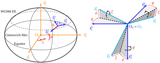
Figure 1. ECEF (${\displaystyle {\mathrm{F}}_{\mathbf{E}}}$), NED (${\displaystyle {\mathrm{F}}_{\mathrm{N}}}$), and body (${\displaystyle {\mathrm{F}}_{\mathrm{B}}}$) reference frames.

This article makes use of the space of rigid body rotations and, hence, relies on the Lie algebra of the special orthogonal group of ${\displaystyle {\mathbb{R}}^3}$, known as ${\displaystyle \mathbb{SO}\left(3\right)}$; refs. [3,4,5] are recommended as references. Generic rotations are represented by ${\displaystyle \mathcal{R}}$ and usually parameterized by the unit quaternion ${\displaystyle \mathbf{q}}$, although the direct cosine matrix ${\displaystyle \mathrm{R}}$ is also employed as required; tangent space representations include the rotation vector ${\displaystyle \mathbf{r}}$ and the angular velocity ${\displaystyle \mathit{w}}$. Related symbols include the quaternion conjugate ${\displaystyle <{·}^{\ast }>}$, the quaternion product ${\displaystyle \otimes }$, and the ${\displaystyle \mathbb{SO}\left(3\right)}$ plus ${\displaystyle \oplus }$ and minus ${\displaystyle \ominus }$ operators.

Superindexes are employed over vectors to specify the frame in which they are viewed (e.g., ${\displaystyle {\mathbf{v}}^{\mathrm{N}}}$ refers to ground velocity viewed in ${\displaystyle {\mathrm{F}}_{\mathrm{N}}}$, while ${\displaystyle {\mathbf{v}}^{\mathrm{B}}}$ is the same vector but viewed in ${\displaystyle {\mathrm{F}}_{\mathrm{B}}}$). Subindexes may be employed to clarify the meaning of a variable or vector, but may also indicate a given vector component; e.g., ${\displaystyle {\mathbf{v}}_2^{\mathrm{N}}}$ refers to the second component of ${\displaystyle {\mathbf{v}}^{\mathrm{N}}}$. In addition, where two reference frames appear as subindexes to a vector, it means that the vector goes from the first frame to the second. For example, ${\displaystyle {\mathit{w}}_{\mathrm{NB}}^{\mathrm{B}}}$ refers to the angular velocity from ${\displaystyle {\mathrm{F}}_{\mathrm{N}}}$ to ${\displaystyle {\mathrm{F}}_{\mathrm{B}}}$ viewed in ${\displaystyle {\mathrm{F}}_{\mathrm{B}}}$. Jacobians are represented by a ${\displaystyle \mathrm{J}}$ combined with a subindex and a superindex; the former identifies the function domain, while the latter applies to the function image or codomain.

3. GNSS-Denied Navigation and Visual Inertial Odometry

The number, variety, and applications of unmanned air vehicles (UAVs) have grown exponentially in the last few years, and the trend is expected to continue in the future [6,7]. A comprehensive review of small UAV navigation systems and the problems they face is included in [8]. The use of GNSS constitutes one of the main enablers for autonomous inertial navigation [9,10,11], but it is also one of its main weaknesses, as in the absence of GNSS signals, inertial systems are forced to rely on dead reckoning, which results in position drift, with the aircraft slowly but steadily deviating from its intended route [2,12]. The availability of GNSS signals cannot be guaranteed; a thorough analysis of GNSS threats and reasons for signal degradation is presented in [13].

At this time, there are no comprehensive solutions to the operation of autonomous UAVs in GNSS-denied scenarios, for which the permanent loss of the GNSS signals is equivalent to losing the airframe in an uncontrolled way. A summary of the challenges of GNSS-denied navigation and the research efforts intended to improve its performance is provided by [2,14,15]. Two promising techniques for completely eliminating the position drift are the use of signals of opportunity [16,17,18] (existing signals originally intended for other purposes, such as those of television and cellular networks, can be employed to triangulate the aircraft position) and georegistration [19,20,21,22,23,24,25,26,27] (the position drift can be eliminated by matching landmarks or terrain features as viewed from the aircraft to preloaded data), also known as image registration.

Visual odometry (VO) consists in employing the ground images generated by one or more onboard cameras without the use of prerecorded image databases or any other sensors, incrementally estimating the vehicle pose (position plus attitude) based on the changes that its motion induces on the images [28,29,30,31,32]. It requires sufficient illumination, dominance of static scene, enough texture, and scene overlap between consecutive images or frames. Modern standalone algorithms, such as semidirect visual odometry (SVO) [33,34], direct sparse odometry (DSO) [35], large-scale direct simultaneous localization and mapping (LSD-SLAM) [36], and large-scale feature-based SLAM (ORB-SLAM) [37,38,39] (ORB stands for oriented FAST and rotated BRIEF, a type of blob feature), are robust and exhibit a limited drift. The incremental concatenation of relative poses results in a slow but unbounded pose drift that disqualifies VO for long-distance autonomous UAV GNSS-denied navigation.

A promising research path to GNSS-denied navigation appears to be the fusion of inertial and visual odometry algorithms into an integrated navigation system. Two different trends coexist in the literature, although an implementation of either group can sometimes employ a technique from the other:

• The first possibility, known as filtering, consists in employing the visual estimations as additional observations with which to feed the inertial filter. In the case of attitude estimation exclusively (momentarily neglecting the platform position), the GNSS signals are helpful and enable the inertial navigation system to obtain more accurate and less noisy estimations, but they are not indispensable, as driftless attitude estimations can be obtained based on the inertial measurement unit (IMU) without their use [2]. Proven techniques for attitude estimation in all kinds of platforms that do not rely on GNSS signals include Gaussian filters [40], deterministic filters [41], complimentary filters [42], and stochastic filters [43,44]. In the case of the complete pose estimation (both attitude and position), it is indispensable to employ the velocity or incremental position observations obtained with VO methods in the absence of the absolute references provided by GNSS receivers. The literature includes cases based on Gaussian filters [45] and, more recently, nonlinear deterministic filters [46], stochastic filters [47], Riccati observers [48], and invariant extended Kalman filters, or EKFs [49].
• The alternative is to employ VO optimizations with the assistance of the inertial navigation estimations, reducing the pose estimation drift inherent to VO. This is known as visual inertial odometry (VIO) [50,51], which can also be combined with image registration to fully eliminate the remaining pose drift. A previous article by the authors, [1], describes how the nonlinear VO optimizations can be enhanced by adding priors based on the inertial attitude and altitude estimations. VIO has matured significantly in the last few years, with detailed reviews available in [50,51,52,53,54].

There exist several open-source VIO packages, such as the multistate constraint Kalman filter (MSCKF) [55], the open keyframe visual inertial SLAM (OKVIS) [56,57], the robust visual inertial odometry (ROVIO) [58], the monocular visual inertial navigation system (VINS-Mono) [59], SVO combined with multisensor fusion (MSF) [33,34,60,61], and SVO combined with incremental smoothing and mapping (iSAM) [33,34,62,63]. All these open-source pipelines are compared in [50], and their results, when applied to the EuRoC micro air vehicles (MAV) data sets, ref. [64] are discussed in [65]. There also exist various other published VIO pipelines with implementations that are not publicly available [66,67,68,69,70,71,72], and there are also others that remain fully proprietary.

The existing VIO schemes to fuse the visual and inertial measurements can be broadly grouped into two paradigms: loosely coupled pipelines process the measurements separately, resulting in independent visual and inertial pose estimations, which are then fused to obtain the final estimate [73,74]; on the other hand, tightly coupled methods compute the final pose estimation directly from the tracked image features and the IMU outputs [50,51]. Tightly coupled approaches usually result in higher accuracy, as they use all the information available and take advantage of the IMU integration to predict the feature locations in the next frame. Loosely coupled methods, although less complex and more computationally efficient, lose information by decoupling the visual and inertial constraints, and are incapable of correcting the drift present in the visual estimator.

A different classification involves the number of images involved in each estimation [50,51,75], which is directly related with the resulting accuracy and computing demands. Batch algorithms, also known as smoothers, estimate multiple states simultaneously by solving a large nonlinear optimization problem or bundle adjustment, resulting in the highest possible accuracy. Valid techniques to limit the required computing resources include the reliance on a subset of the available frames (known as keyframes), the separation of tracking and mapping into different threads, and the development of incremental smoothing techniques based on factor graphs [63]. Although employing all available states (full smoothing) is sometimes feasible for very short trajectories, most pipelines rely on sliding window or fixed lag smoothing, in which the optimization relies exclusively on the measurements associated with the last few keyframes, discarding both the old keyframes and other frames that have not been cataloged as keyframes. On the other hand, filtering algorithms restrict the estimation process to the latest state; they require less resources but suffer from permanently dropping all previous information and a much harder identification and removal of outliers, both of which lead to error accumulation or drift.

Additional VIO pipelines are also being developed to take advantage of event cameras [76,77], which measure per-pixel luminosity changes asynchronously instead of capturing images at a fixed rate. Event cameras hold very advantageous properties for visual odometry, including low latency, very high frequency, and excellent dynamic range, which make them well suited to deal with high-speed motion and high dynamic range, which are problematic for traditional VO and VIO pipelines. On the negative side, new algorithms are required to cope with the sequence of asynchronous events they generate [50].

4. Novelty

The main novelty of this article (second phase of the fusion between the inertial and visual navigation systems) lies in the following two topics:

• The use of a modified EKF scheme within the navigation filter (Section 8) based on Lie algebra to ensure that the estimated aircraft body attitude is propagated along its tangent space and never deviates from its ${\displaystyle \mathbb{SO}\left(3\right)}$ manifold, reducing the error growth inherent to concatenating estimations over a long period of time.
• The transformation within the VVS (Section 7) of the position estimations obtained by the visual system into incremental displacement measurements, which are unbiased and hence more adequate to be used as observations within an EKF.

When comparing the integrated system (which includes both [1] and this article) with the state of the art discussed in Section 3, the proposed approach combines the high accuracy representative of tightly coupled smoothers with the lack of complexity and reduced computing requirements of filters and loosely coupled systems. The existence of two independent solutions (inertial and visual) hints to a loosely coupled approach, but in fact, the proposed solution shares most traits with tightly coupled pipelines:

• No information is discarded because the two solutions are not independent, as each simultaneously feeds and is fed by the other. The visual estimations depend on the inertial outputs, while the inertial filter uses the visual incremental displacement estimations as observations. Unlike loosely coupled solutions, the visual estimations for attitude and altitude are not allowed to deviate from the inertial ones above a certain threshold, so they do not drift.
• The two estimations are never fused together, as the inertial solution constitutes the final output, while the sole role of the visual outputs is to act as the previously mentioned incremental sensor.

With respect to the last criterion found in Section 3, the proposed approach contains both a filter within the inertial system and a keyframe-based sliding window smoother within the visual one, obtaining the best properties of both categories.

5. Application

The visual inertial solutions listed in Section 3 are quite generic with respect to the platforms on which they are mounted, with most applications focused on the short distance trajectories of ground vehicles, indoor robots, and multirotors, as well as with respect to the employed sensors, which are usually restricted to the IMU and one or more cameras. The proposed approach differs in its more restricted application, as it focuses on the specific case of long-distance GNSS-denied turbulent flight of fixed-wing autonomous aircraft:

• Being restricted to aerial vehicles, it takes advantage of the extra sensors already present on board these platforms, such as magnetometers and barometer.
• The fixed-wing limitation is caused by the visual system relying on the pitot tube to continue navigating when overflying texture-poor terrain [1].
• As exemplified by the two scenarios employed to evaluate the algorithms, the proposed approach can cope with heavy turbulence, which increases the platform accelerations as well as the optical flow between consecutive images. Although not discussed in the results, the turbulence level has a negligible effect on the navigation accuracy as long as it remains below a sufficiently elevated threshold.
• With the exception of atmospheric pressure changes, which accumulate as vertical position estimation errors (Section 10.2), weather changes such as wind and atmospheric temperature have no effect on the navigation accuracy.
• It focuses more on GNSS-denied environments of a different nature than those experienced by other platforms, as it can always be assumed that GNSS signals are present at the beginning of the flight, and if they disappear, the reason is likely to be technical error or intentional action, so the vehicle needs to be capable of flying for long periods of time in GNSS-denied conditions.
• The reliance on visual navigation imposes certain restrictions, such as the need for sufficient illumination, lack of cloud cover below the aircraft, and impossibility to navigate over large bodies of water. The use of infrared cameras, although out of the scope of this article, is a promising research area for the first two restrictions, but the lack of static features makes visual systems inadequate for navigation over water.

6. Proposed Visual Inertial Navigation Architecture

The navigation system processes the measurements of the various onboard sensors (${\displaystyle \tilde{\mathbf{x}}={\mathbf{x}}_{\mathrm{SENSED}}}$) and generates the estimated state (${\displaystyle \widehat{\mathbf{x}}={\mathbf{x}}_{\mathrm{EST}}}$) required by the guidance and control systems, which contains an estimation of the true aircraft state ${\displaystyle \mathbf{x}={\mathbf{x}}_{\mathrm{TRUTH}}}$. Note that in this article, the images ${\displaystyle \mathbf{I}}$ are considered part of the sensed states ${\displaystyle \tilde{\mathbf{x}}={\mathbf{x}}_{\mathrm{SENSED}}}$ as the camera is treated as an additional sensor. Hardware and computing power limitations often require the camera and visual algorithms to operate at a lower frequency than those of inertial algorithms and the remaining sensors. Table 1 includes the operating frequencies employed to generate the Section 10 results. Note that the index t identifies a discrete time instant (${\displaystyle {\mathrm{t}}_{\mathrm{t}}}$) for the aircraft trajectory, s (${\displaystyle {\mathrm{t}}_{\mathrm{s}}}$) refers to the sensor outputs, n (${\displaystyle {\mathrm{t}}_{\mathrm{n}}}$) identifies an inertial estimation, c (${\displaystyle {\mathrm{t}}_{\mathrm{c}}}$) is a control system execution, i (${\displaystyle {\mathrm{t}}_{\mathrm{i}}}$) applies to a camera image and the corresponding visual estimation, and g (${\displaystyle {\mathrm{t}}_{\mathrm{g}}}$) refers to a GNSS receiver observation.

Table 1. Working frequencies of the different systems.

Discrete Time	Frequency	Variable	System
${\displaystyle {\mathrm{t}}_{\mathrm{t}}=\mathrm{t}·\Delta {\mathrm{t}}_{\mathrm{TRUTH}}}$	${\displaystyle 500\mathrm{Hz}}$	${\displaystyle \mathbf{x}={\mathbf{x}}_{\mathrm{TRUTH}}}$	Flight physics
${\displaystyle {\mathrm{t}}_{\mathrm{s}}=\mathrm{s}·\Delta {\mathrm{t}}_{\mathrm{SENSED}}}$	${\displaystyle 100\mathrm{Hz}}$	${\displaystyle \tilde{\mathbf{x}}={\mathbf{x}}_{\mathrm{SENSED}}}$	Sensors
${\displaystyle {\mathrm{t}}_{\mathrm{n}}=\mathrm{n}·\Delta {\mathrm{t}}_{\mathrm{EST}}}$	${\displaystyle 100\mathrm{Hz}}$	${\displaystyle \widehat{\mathbf{x}}={\mathbf{x}}_{\mathrm{EST}}}$	Inertial navigation
${\displaystyle {\mathrm{t}}_{\mathrm{c}}=\mathrm{c}·\Delta {\mathrm{t}}_{\mathrm{CNTR}}}$	${\displaystyle 50\mathrm{Hz}}$	${\displaystyle {\mathbf{\delta }}_{\mathrm{TARGET}},{\mathbf{\delta }}_{\mathrm{CNTR}}}$	Guidance and control
${\displaystyle {\mathrm{t}}_{\mathrm{i}}=\mathrm{i}·\Delta {\mathrm{t}}_{\mathrm{IMG}}}$	${\displaystyle 10\mathrm{Hz}}$	${\displaystyle {\mathbf{x}}_{\mathrm{IMG}}}$	Visual navigation and camera
${\displaystyle {\mathrm{t}}_{\mathrm{g}}=\mathrm{g}·\Delta {\mathrm{t}}_{\mathrm{GNSS}}}$	${\displaystyle 1\mathrm{Hz}}$		GNSS receiver

The proposed strategy to fuse the inertial and visual navigation systems is based on their performances as standalone systems [1,2], as summarized in Table 2. Inertial systems are clearly superior to visual ones in GNSS-denied attitude and altitude estimation since their estimations are bounded and do not drift. In the case of horizontal position, both systems drift and are hence inappropriate for long-term GNSS-denied navigation, but for different reasons; while the inertial drift is the result of integrating the bounded ground velocity estimations without absolute position observations, the visual one originates on the slow but continuous accumulation of estimation errors between consecutive images.

Table 2. Summary of inertial and visual standalone navigation systems.

GNSS-Denied	Inertial	Visual
Attitude	Bounded by sensor quality	Drifts
	Yaw worse than pitch and bank	Yaw better than pitch and bank
Vertical	Bounded by atmospheric physics	Drifts
Horizontal	Drifts	Drifts

It is also worth noting that inertial estimations are significantly noisier than visual ones, so the latter, although worse on an absolute basis, are often more accurate when evaluating the estimations incrementally, this is, from one image to the next or even for the time interval corresponding to a few images. When applied to the horizontal position, the high accuracy of the incremental image-to-image displacement observations (equivalent to ground velocity observations) constitutes the basis for the second phase of the fusion described in the following sections.

This article proposes an inertial navigation filter (Section 8) that, in the absence of GNSS signals, takes advantage of the incremental displacement outputs generated by a visual system as if they were the observations generated by an additional sensor (Section 7), denoted as the virtual vision sensor, or VVS. The proposed EKF relies on the observations provided by the onboard accelerometers, gyroscopes, and magnetometers, combined with those of the GNSS receiver when signals are available, or those of the VVS when they are not. The inertial navigation filter and the visual system continuously assist and control each other, as depicted in Figure 2. As the integrated system needs to estimate the state ${\displaystyle \widehat{\mathbf{x}}={\mathbf{x}}_{\mathrm{EST}}}$ at every ${\displaystyle {\mathrm{t}}_{\mathrm{n}}={\mathrm{t}}_{\mathrm{s}}=\mathrm{n}·\Delta {\mathrm{t}}_{\mathrm{EST}}=\mathrm{s}·\Delta {\mathrm{t}}_{\mathrm{SENSED}}}$, it has three different operation modes, depending not only on whether GNSS signals are available or not, but also on whether there exist a position and ground velocity observation at the execution time ${\displaystyle {\mathrm{t}}_{\mathrm{n}}={\mathrm{t}}_{\mathrm{s}}}$:

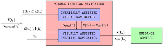
Figure 2. Proposed visual inertial navigation system flow diagram.

• Given the operating frequencies of the different sensors listed in Table 1, most navigation filter cycles (99 out of 100 for GNSS-based navigation, 9 out of 10 in case of GNSS-denied conditions) can not rely on the position and ground velocity observations provided by either the GNSS receiver or the VVS. These cycles successively apply the EKF time update, measurement update, and reset equations (Section 8), noting that the filter observation system needs to be simplified by removing the ground velocity and position observations, which are not available.
• GNSS-denied filter cycles for which the VVS position and ground velocity observations are available at the required time (${\displaystyle {\mathrm{t}}_{\mathrm{n}}=\mathrm{n}·\Delta {\mathrm{t}}_{\mathrm{EST}}={\mathrm{t}}_{\mathrm{i}}=\mathrm{i}·\Delta {\mathrm{t}}_{\mathrm{IMG}}}$) rely on the Figure 3 scheme. Note that this case only occurs in 1 out of 10 executions for GNSS-denied conditions. The first part of the process is exactly the same as in the previous case, estimating first the a priori state and covariance (${\displaystyle {\widehat{\mathbf{x}}}_{\mathrm{n}}^{-}}$, ${\displaystyle {\mathbf{P}}_{\mathrm{n}}^{-}}$), followed by the a posteriori ones (${\displaystyle {\widehat{\mathbf{x}}}_{\mathrm{PRE},\mathrm{n}}^{+}}$, ${\displaystyle {\mathbf{P}}_{\mathrm{PRE},\mathrm{n}}^{+}}$), and finally the estimated state (${\displaystyle {\widehat{\mathbf{x}}}_{\mathrm{PRE}}\left({\mathrm{t}}_{\mathrm{n}}\right)={\mathbf{x}}_{\mathrm{EST},\mathrm{PRE}}\left({\mathrm{t}}_{\mathrm{n}}\right)}$). Note that as these estimations do not employ the VVS measurements (that is, do not employ the ${\displaystyle {\mathrm{I}}_{\mathrm{i}}}$ image corresponding to ${\displaystyle {\mathrm{t}}_{\mathrm{i}}}$), they are preliminary and hence denoted with the subindex PRE to avoid confusion.
  

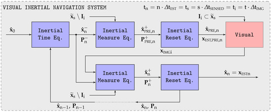  Figure 3. Navigation filter flow diagram when ${\displaystyle {\mathrm{t}}_{\mathrm{n}}={\mathrm{t}}_{\mathrm{s}}={\mathrm{t}}_{\mathrm{i}}}$.
  The preliminary estimation ${\displaystyle {\widehat{\mathbf{x}}}_{\mathrm{PRE},\mathrm{n}}={\mathbf{x}}_{\mathrm{EST},\mathrm{PRE},\mathrm{n}}}$ together with the ${\displaystyle {\mathbf{I}}_{\mathrm{i}}}$ image is then passed to the visual system [1] to obtain a visual state ${\displaystyle {\mathbf{x}}_{\mathrm{IMG}}\left({\mathrm{t}}_{\mathrm{i}}\right)}$, which, as explained in Section 7, is equivalent to the VVS position and ground velocity outputs. Only then it is possible to apply the complete navigation filter measurement update and reset equations for a second time to obtain the final state estimation ${\displaystyle \widehat{\mathbf{x}}\left({\mathrm{t}}_{\mathrm{n}}\right)={\mathbf{x}}_{\mathrm{EST}}\left({\mathrm{t}}_{\mathrm{n}}\right)}$.
• GNSS-based filter cycles for which the GNSS receiver position and ground velocity observations are available at the required time (${\displaystyle {\mathrm{t}}_{\mathrm{n}}=\mathrm{n}·\Delta {\mathrm{t}}_{\mathrm{EST}}={\mathrm{t}}_{\mathrm{g}}=\mathrm{g}·\Delta {\mathrm{t}}_{\mathrm{GNSS}}}$). This case, which only occurs in one out of a hundred executions when GNSS signals are available, is in fact very similar to the first one above, with the only difference being that the navigation filter observation system does not need any simplifications.

7. Virtual Vision Sensor

The virtual vision sensor (VVS) constitutes an alternative denomination for the incremental displacement outputs obtained by the inertial assisted visual system described in [1]. Its horizontal position estimations drift with time due to the absence of absolute observations, but when evaluated on an incremental basis, that is, from one image to the next, the incremental displacement estimations are quite accurate. This section shows how to convert these incremental estimations into measurements for the geodetic coordinates (${\displaystyle {\tilde{\mathbf{T}}}^{\mathbf{E},\mathrm{GDT}}}$) and the ${\displaystyle {\mathrm{F}}_{\mathrm{N}}}$ ground velocity (${\displaystyle {\tilde{\mathbf{v}}}^{\mathrm{N}}}$), so the VVS can smoothly replace the GNSS receiver within the navigation filter in the absence of GNSS signals (Section 8).

Their obtainment relies on the current visual state ${\displaystyle {\mathbf{x}}_{\mathrm{IMG}}\left({\mathrm{t}}_{\mathrm{i}}\right)={\mathbf{x}}_{\mathrm{IMG},\mathrm{i}}}$ generated by the visual system, the one obtained with the previous frame ${\displaystyle {\mathbf{x}}_{\mathrm{IMG}}\left({\mathrm{t}}_{\mathrm{i}-1}\right)={\mathbf{x}}_{\mathrm{IMG},\mathrm{i}-1}}$, as well as the estimated state ${\displaystyle \widehat{\mathbf{x}}\left({\mathrm{t}}_{\mathrm{n}-\delta \mathrm{t}}\right)}$ = ${\displaystyle {\mathbf{x}}_{\mathrm{EST}}\left({\mathrm{t}}_{\mathrm{n}-\delta \mathrm{t}}\right)}$ = ${\displaystyle {\widehat{\mathbf{x}}}_{\mathrm{n}-\delta \mathrm{t}}}$ corresponding to the previous image generated by the inertial system. Note that as ${\displaystyle \mathrm{t}={\mathrm{t}}_{\mathrm{i}}}$ = ${\displaystyle \mathrm{i}·\Delta {\mathrm{t}}_{\mathrm{IMG}}}$ = ${\displaystyle {\mathrm{t}}_{\mathrm{n}}=\mathrm{n}·\Delta {\mathrm{t}}_{\mathrm{EST}}}$, the relationship between i and n is as follows, where ${\displaystyle \delta \mathrm{t}=10}$ is the number of inertial executions for every image being processed (Table 1):

$$\mathrm{n}=\mathrm{i}·\frac{\Delta {\mathrm{t}}_{\mathrm{IMG}}}{\Delta {\mathrm{t}}_{\mathrm{EST}}}=\mathrm{i}·\delta \mathrm{t}$$

(1)

• To obtain the VVS velocity observations (${\displaystyle {\tilde{\mathbf{v}}}^{\mathrm{N}}}$), it is necessary to first compute the geodetic coordinate (longitude ${\displaystyle \lambda }$, latitude ${\displaystyle \phi }$, altitude h) time derivative based on the difference between their values corresponding to the last two images (2), followed by their transformation into ${\displaystyle {\tilde{\mathbf{v}}}^{\mathrm{N}}}$ per (3), in which M and N represent the WGS84 radii of curvature of meridian and prime vertical, respectively. Note that ${\displaystyle {\tilde{\mathbf{v}}}^{\mathrm{N}}}$ is very noisy given how it is obtained.

  $$\begin{array}{ccc}\hfill {\dot{\mathbf{T}}}_{\mathrm{IMG},\mathrm{i}}^{\mathbf{E},\mathrm{GDT}}& =& {\left[{\dot{\lambda }}_{\mathrm{IMG},\mathrm{i}}{\dot{\phi }}_{\mathrm{IMG},\mathrm{i}}{\dot{\mathrm{h}}}_{\mathrm{IMG},\mathrm{i}}\right]}^{\mathrm{T}}=\frac{{\mathbf{T}}_{\mathrm{IMG},\mathrm{i}}^{\mathbf{E},\mathrm{GDT}}-{\mathbf{T}}_{\mathrm{IMG},\mathrm{i}-1}^{\mathbf{E},\mathrm{GDT}}}{\Delta {\mathrm{t}}_{\mathrm{IMG}}}\hfill \end{array}$$

  (2)

  $$\begin{array}{ccc}\hfill {\tilde{\mathbf{v}}}_{\mathrm{n}}^{\mathrm{N}}& =& \left[\begin{array}{c}\left[\mathrm{M}\left({\tilde{\phi }}_{\mathrm{n}-\delta \mathrm{t}}\right)+{\tilde{\mathrm{h}}}_{\mathrm{n}-\delta \mathrm{t}}\right]{\dot{\phi }}_{\mathrm{IMG},\mathrm{i}}\\ \left[\mathrm{N}\left({\tilde{\phi }}_{\mathrm{n}-\delta \mathrm{t}}\right)+{\tilde{\mathrm{h}}}_{\mathrm{n}-\delta \mathrm{t}}\right]cos{\tilde{\phi }}_{\mathrm{n}-\delta \mathrm{t}}{\dot{\lambda }}_{\mathrm{IMG},\mathrm{i}}\\ -{\dot{\mathrm{h}}}_{\mathrm{IMG},\mathrm{i}}\end{array}\right]\hfill \end{array}$$

  (3)
• With respect to the VVS geodetic coordinates, the sensed longitude and latitude can be obtained per (5) and (6) based on propagating the previous inertial estimations (those corresponding to the time of the previous VVS reading) with their visually obtained time derivatives. To avoid drift, the geometric altitude ${\displaystyle \tilde{\mathrm{h}}}$ is estimated based on the barometer observations assuming that the atmospheric pressure offset remains frozen from the time the GNSS signals are lost [2].

  $$\begin{array}{ccc}\hfill {\tilde{\mathbf{T}}}_{\mathrm{n}}^{\mathbf{E},\mathrm{GDT}}& =& {\left[{\tilde{\lambda }}_{\mathrm{n}}{\tilde{\phi }}_{\mathrm{n}}{\tilde{\mathrm{h}}}_{\mathrm{n}}\right]}^{\mathrm{T}}\hfill \end{array}$$

  (4)

  $$\begin{array}{ccc}\hfill {\tilde{\lambda }}_{\mathrm{n}}& =& {\widehat{\lambda }}_{\mathrm{n}-\delta \mathrm{t}}+{\dot{\lambda }}_{\mathrm{IMG},\mathrm{i}}\Delta {\mathrm{t}}_{\mathrm{IMG}}\hfill \end{array}$$

  (5)

  $$\begin{array}{ccc}\hfill {\tilde{\phi }}_{\mathrm{n}}& =& {\widehat{\phi }}_{\mathrm{n}-\delta \mathrm{t}}+{\dot{\phi }}_{\mathrm{IMG},\mathrm{i}}\Delta {\mathrm{t}}_{\mathrm{IMG}}\hfill \end{array}$$

  (6)

With respect to the covariances, the authors have assigned the VVS an ad hoc position standard deviation one order of magnitude lower than that employed for the GNSS receiver so the navigation filter (Section 8) closely tracks the position observations provided by the VVS. Given the noisy nature of the virtual velocity observations, the authors have preferred to employ a dynamic evaluation for the velocity standard deviation, which coincides with the absolute value (for each of the three dimensions) of the difference between each new velocity observation and the running average of the last 20 readings (equivalent to the last ${\displaystyle 2\mathrm{s}}$). In this way, when GNSS signals are available, the covariance of the position observations is higher, so the navigation filter slowly corrects the position estimations obtained from integrating the state equations instead of closely adhering to the noisy GNSS position measurements; when GNSS signals are not present, the VVS low position observation covariance combined with the high-velocity one implies that the navigation EKF (Section 8) closely tracks the VVS position readings (4), continuously adjusting the aircraft velocity estimations with little influence from the VVS velocity observations in order to complement its position estimations.

8. Proposed Navigation Filter

As graphically depicted in Figure 2, the navigation filter estimates the aircraft pose ${\displaystyle \widehat{\mathbf{x}}={\mathbf{x}}_{\mathrm{EST}}}$ based on the observations provided by the onboard sensors with the exception of the camera, ${\displaystyle \tilde{\mathbf{x}}\setminus \mathbf{I}={\mathbf{x}}_{\mathrm{SENSED}}\setminus \mathbf{I}}$, complemented if necessary (in the absence of GNSS signals) by the visual observations ${\displaystyle {\mathbf{x}}_{\mathrm{IMG}}}$ provided by the VVS. Implemented as an EKF, the objective of the navigation filter is the estimation of the aircraft attitude between the ${\displaystyle {\mathrm{F}}_{\mathrm{N}}}$ and ${\displaystyle {\mathrm{F}}_{\mathrm{B}}}$ frames represented by its unit quaternion ${\displaystyle {\widehat{\mathbf{q}}}_{\mathrm{NB}}}$[3] together with the aircraft position represented by its geodetic coordinates ${\displaystyle {\widehat{\mathbf{T}}}^{\mathbf{E},\mathrm{GDT}}}$. Additional state vector members include the aircraft angular velocity ${\displaystyle {\widehat{\mathit{w}}}_{\mathrm{NB}}^{\mathrm{B}}}$; the ground velocity ${\displaystyle {\widehat{\mathbf{v}}}^{\mathrm{N}}}$; the specific force ${\displaystyle {\widehat{\mathbf{f}}}_{\mathrm{IB}}^{\mathrm{B}}}$ or nongravitational acceleration from ${\displaystyle {\mathrm{F}}_{\mathrm{I}}}$ to ${\displaystyle {\mathrm{F}}_{\mathrm{B}}}$; the full gyroscope, accelerometer, and magnetometer errors (${\displaystyle {\widehat{\mathbf{E}}}_{\mathrm{GYR}},{\widehat{\mathbf{E}}}_{\mathrm{ACC}},{\widehat{\mathbf{E}}}_{\mathrm{MAG}}}$) that include all sensor error sources except system noise; and the difference ${\displaystyle {\widehat{\mathbf{B}}}_{\mathrm{DEV}}^{\mathrm{N}}}$ between the Earth magnetic field provided by the onboard model ${\displaystyle {\mathbf{B}}_{\mathrm{MOD}}^{\mathrm{N}}}$ and the real one ${\displaystyle {\mathbf{B}}_{\mathrm{REAL}}^{\mathrm{N}}}$.

$$\mathbf{x}\left(\mathrm{t}\right)={\left[{\mathbf{q}}_{\mathrm{NB}}{\mathit{w}}_{\mathrm{NB}}^{\mathrm{B}}{\mathbf{T}}^{\mathrm{E},\mathrm{GDT}}{\mathbf{v}}^{\mathrm{N}}{\mathbf{f}}_{\mathrm{IB}}^{\mathrm{B}}{\mathbf{E}}_{\mathrm{GYR}}{\mathbf{E}}_{\mathrm{ACC}}{\mathbf{E}}_{\mathrm{MAG}}{\mathbf{B}}_{\mathrm{DEV}}^{\mathrm{N}}\right]}^{\mathbf{T}}$$

(7)

Rigid body rotations are characterized by their orthogonality (they preserve the norm of vectors and the angle between vectors) and their handedness (they preserve the orientation or cross product between vectors); when encoded as quaternions, these two constraints converge into a single one, the unitary norm, as only unit quaternions are valid parameterizations of rigid body rotations [3,4,5]. As the body attitude ${\displaystyle {\mathbf{q}}_{\mathrm{NB}}}$ belongs to the non-Euclidean special orthogonal group or ${\displaystyle \mathbb{SO}\left(3\right)}$, the classical EKF scheme [78], which relies on linear algebra, shall be replaced by the alternative formulation proposed here to ensure that the estimated attitude never deviates from its ${\displaystyle \mathbb{SO}\left(3\right)}$ manifold, that is, to ensure that ${\displaystyle {\mathbf{q}}_{\mathrm{NB}}}$ remains unitary at all times [79]. Relying on linear algebra implies treating the unit quaternion ${\displaystyle {\mathbf{q}}_{\mathrm{NB}}}$ as a 4-vector in both the time update and measurement update equations of each EKF cycle, and then normalizing the resulting nonunit quaternion at the end of each cycle; although this is an established practice that provides valid results when operating at the high frequencies typical of inertial sensors, the slower frequencies characteristic of visual pipelines (refer to ${\displaystyle \Delta {\mathrm{t}}_{\mathrm{SENSED}}}$ and ${\displaystyle \Delta {\mathrm{t}}_{\mathrm{IMG}}}$ in Table 1) when combined with the lack of absolute position observations in the absence of GNSS signals result in slight but non-negligible inaccuracies in each cycle, which can accumulate into significant errors when the aircraft needs to navigate without absolute position observations for long periods of time.

The use of Lie theory, with its manifolds and tangent spaces, enables the construction of rigorous calculus techniques to handle uncertainties, derivatives, and integrals of non-Euclidean elements with precision and ease [4]. Lie theory can hence be employed to generate an alternative EKF scheme suitable for state vectors containing non-Euclidean components [5]. This alternative EKF scheme differs in four key points from the classical Euclidean one; these four differences are discussed in the following paragraphs. Note that the GNSS-denied navigation results discussed in Section 10 cannot be obtained without the use of Lie algebra and the alternative EKF formulation.

The most rigorous and precise way to adapt the EKF scheme to the presence of non-Euclidean elements, such as rigid body rotations, is to exclude the rotation element ${\displaystyle {\mathbf{q}}_{\mathrm{NB}}\in \mathbb{SO}\left(3\right)}$ from the state vector, replacing the unit quaternion ${\displaystyle {\mathbf{q}}_{\mathrm{NB}}}$ by a local (${\displaystyle {\mathrm{F}}_{\mathrm{B}}}$) tangent space perturbation represented by the rotation vector ${\displaystyle \Delta {\mathbf{r}}_{\mathrm{NB}}^{\mathrm{B}}\in {\mathbb{R}}^3}$[4,5]. Note that the state vector (9) includes the velocity of ${\displaystyle {\mathbf{q}}_{\mathrm{NB}}}$ as it moves along its manifold (its angular velocity ${\displaystyle {\mathit{w}}_{\mathrm{NB}}^{\mathrm{B}}}$), also contained in the local (${\displaystyle {\mathrm{F}}_{\mathrm{B}}}$) tangent space. Each filter step now consists in estimating the rotation element ${\displaystyle {\widehat{\mathbf{q}}}_{\mathrm{NB}\mathrm{n}}={\widehat{\mathbf{q}}}_{\mathrm{NB}}\left({\mathrm{t}}_{\mathrm{n}}\right)\in \mathbb{SO}\left(3\right)}$, the state vector ${\displaystyle {\widehat{\mathbf{x}}}_{\mathrm{n}}=\widehat{\mathbf{x}}\left({\mathrm{t}}_{\mathrm{n}}\right)={\left[\Delta {\widehat{\mathbf{r}}}_{\mathrm{NB}\mathrm{n}}^{\mathrm{B}}{\widehat{}}_{\mathrm{NB}\mathrm{n}}^{\mathrm{B}}{\widehat{\mathbf{z}}}_{\mathrm{n}}\right]}^{\mathrm{T}}\in {\mathbb{R}}^{27}}$, and its covariance ${\displaystyle {\mathbf{P}}_{\mathrm{n}}=\mathbf{P}\left({\mathrm{t}}_{\mathrm{n}}\right)\in {\mathbb{R}}^{27\times 27}}$, based on their values at ${\displaystyle {\mathrm{t}}_{\mathrm{n}-1}=\left(\mathrm{n}-1\right)\Delta \mathrm{t}}$ and the observations at ${\displaystyle {\mathrm{t}}_{\mathrm{n}}=\mathrm{n}\Delta \mathrm{t}}$.

$$\mathcal{R}\left(\mathrm{t}\right)={\mathbf{q}}_{\mathrm{NB}}\in \mathbb{SO}\left(3\right)\left(\mathrm{t}\right)$$

(8)

$$\begin{array}{ccc}\hfill \mathbf{x}\left(\mathrm{t}\right)& =& {\left[\Delta {\mathbf{r}}_{\mathrm{NB}}^{\mathrm{B}}{\mathit{w}}_{\mathrm{NB}}^{\mathrm{B}}\mathbf{z}\right]}^{\mathrm{T}}={\left[\Delta {\mathbf{r}}_{\mathrm{NB}}^{\mathrm{B}}\mathbf{p}\right]}^{\mathrm{T}}\hfill \\ & =& {\left[\Delta {\mathbf{r}}_{\mathrm{NB}}^{\mathrm{B}}{\mathit{w}}_{\mathrm{NB}}^{\mathrm{B}}{\mathbf{T}}^{\mathbf{E},\mathrm{GDT}}{\mathbf{v}}^{\mathrm{N}}{\mathbf{f}}_{\mathrm{IB}}^{\mathrm{B}}{\mathbf{E}}_{\mathrm{GYR}}{\mathbf{E}}_{\mathrm{ACC}}{\mathbf{E}}_{\mathrm{MAG}}{\mathrm{B}}_{\mathrm{DEV}}^{\mathrm{N}}\right]}^{\mathrm{T}}\in {\mathbb{R}}^{27}\left(\mathrm{t}\right)\hfill \end{array}$$

(9)

The observations ${\displaystyle {\mathbf{y}}_{\mathrm{n}}}$ are provided by the gyroscopes, which measure the inertial angular velocity ${\displaystyle {\tilde{\mathit{w}}}_{\mathrm{IB}}^{\mathrm{B}}}$, the accelerometers that provide the specific force ${\displaystyle {\tilde{\mathbf{f}}}_{\mathrm{IB}}^{\mathrm{B}}}$ or nongravitational acceleration, the magnetometers that measure the magnetic field ${\displaystyle {\tilde{\mathbf{B}}}^{\mathrm{B}}}$, and either the GNSS receiver or the VVS (Section 7) that provides the position ${\displaystyle {\tilde{\mathbf{T}}}^{\mathrm{E},\mathrm{GDT}}}$ (geodetic coordinates) and ground velocity ${\displaystyle {\tilde{\mathbf{v}}}^{\mathrm{N}}}$ observations. Note that the measurements are provided at different frequencies, as listed in Table 1; most are available every ${\displaystyle \Delta {\mathrm{t}}_{\mathrm{SENSED}}=0.01\mathrm{s}}$, but the ground velocity and position measurements are generated every ${\displaystyle \Delta {\mathrm{t}}_{\mathrm{GNSS}}=1\mathrm{s}}$ if provided by the GNSS receiver or every ${\displaystyle \Delta {\mathrm{t}}_{\mathrm{IMG}}=0.1\mathrm{s}}$ when the GNSS signals are not available and the readings are instead supplied by the VVS.

$$\begin{array}{ccc}\hfill {\mathbf{y}}_{\mathrm{n}}& =& {\left[{\tilde{\mathit{w}}}_{\mathrm{IB}}^{\mathrm{B}}{\tilde{\mathbf{f}}}_{\mathrm{IB}}^{\mathrm{B}}{\tilde{\mathbf{B}}}^{\mathrm{B}}{\tilde{\mathbf{T}}}^{\mathrm{E},\mathrm{GDT}}{\tilde{\mathbf{v}}}^{\mathrm{N}}\right]}^{\mathrm{T}}\in {\mathbb{R}}_{\mathrm{n}}^{15}\hfill \end{array}$$

(10)

8.1. Time Update Equations

The variation with time of the state variables (11) comprises a continuous time nonlinear state system composed of three exact equations (with no simplifications), (12), (14), and (15), together with six other differential Equations (13) and (16) in which the filter does not posses any knowledge about the time derivatives of the state variables, which are hence set to zero. The three exact equations are the following:

• The rotational motion time derivative (12) [4,5];
• The geodetic coordinates kinematics (14);
• The aircraft velocity dynamics (15) [2].

$$\begin{array}{ccc}\hfill \dot{\mathbf{x}}\left(\mathrm{t}\right)& =& {\left[\Delta {\dot{\mathbf{r}}}_{\mathrm{NB}}^{\mathrm{B}}{\dot{\mathit{w}}}_{\mathrm{NB}}^{\mathrm{B}}\dot{\mathbf{z}}\right]}^{\mathrm{T}}=\mathbf{f}\left({\mathbf{q}}_{\mathrm{NB}}\left(\mathrm{t}\right)\oplus \Delta {\mathbf{r}}_{\mathrm{NB}}^{\mathrm{B}}\left(\mathrm{t}\right),{\mathit{w}}_{\mathrm{NB}}^{\mathrm{B}}\left(\mathrm{t}\right),\mathbf{z}\left(\mathrm{t}\right),\mathbf{w}\left(\mathrm{t}\right),\mathrm{t}\right)\hfill \end{array}$$

(11)

$$\begin{array}{ccc}\hfill {\dot{\mathbf{x}}}_{1-3}& =& \Delta {\dot{\mathbf{r}}}_{\mathrm{NB}}^{\mathrm{B}}={\mathit{w}}_{\mathrm{NB}}^{\mathrm{B}}={\mathbf{x}}_{4-6}\hfill \end{array}$$

(12)

$$\begin{array}{ccc}\hfill {\dot{\mathbf{x}}}_{4-6}& =& {\dot{\mathit{w}}}_{\mathrm{NB}}^{\mathrm{B}}=0_3\hfill \end{array}$$

(13)

$$\begin{array}{ccc}\hfill {\dot{\mathbf{x}}}_{7-9}& =& {\dot{\mathbf{T}}}^{\mathbf{E},\mathrm{GDT}}={\left[{\displaystyle \frac{{\mathrm{v}}_2^{\mathrm{N}}}{\left[\mathrm{N}\left(\phi \right)+\mathrm{h}\right]cos\phi }}{\displaystyle \frac{{\mathrm{v}}_1^{\mathrm{N}}}{\mathrm{M}\left(\phi \right)+\mathrm{h}}}-{\mathrm{v}}_3^{\mathrm{N}}\right]}^{\mathrm{T}}\hfill \end{array}$$

(14)

$$\begin{array}{ccc}\hfill {\dot{\mathbf{x}}}_{10-12}& =& {\dot{\mathbf{v}}}^{\mathrm{N}}=\left({\mathbf{q}}_{\mathrm{NB}}\oplus \Delta {\mathbf{r}}_{\mathrm{NB}}^{\mathrm{B}}\right)\otimes {\mathbf{f}}_{\mathrm{IB}}^{\mathrm{B}}\otimes {\left({\mathbf{q}}_{\mathrm{NB}}\oplus \Delta {\mathbf{r}}_{\mathrm{NB}}^{\mathrm{B}}\right)}^{\ast }-{\left[{\mathit{w}}_{\mathrm{EN}}^{\mathrm{N}}\right]}_{\times }{\mathbf{v}}^{\mathrm{N}}+{\mathbf{g}}_{\mathrm{c},\mathrm{MOD}}^{\mathrm{N}}-{\mathbf{a}}_{\mathrm{cor}}^{\mathrm{N}}\hfill \end{array}$$

(15)

$$\begin{array}{ccc}\hfill {\dot{\mathbf{x}}}_{13-27}& =& {\left[{\dot{\mathbf{f}}}_{\mathrm{IB}}^{\mathrm{B}}{\dot{\mathbf{E}}}_{\mathrm{GYR}}{\dot{\mathbf{E}}}_{\mathrm{ACC}}{\dot{\mathbf{E}}}_{\mathrm{MAG}}{\dot{\mathbf{B}}}_{\mathrm{DEV}}^{\mathrm{N}}\right]}^{\mathrm{T}}=0_{15}\hfill \end{array}$$

(16)

Note that in expression (15), ${\displaystyle {\mathit{w}}_{\mathrm{EN}}^{\mathrm{N}}}$ represents the ${\displaystyle {\mathrm{F}}_{\mathrm{N}}}$ motion angular velocity experienced by any object that moves without modifying its attitude with respect to the Earth surface, ${\displaystyle {\mathbf{g}}_{\mathrm{c},\mathrm{MOD}}^{\mathrm{N}}}$ constitutes the gravity acceleration modeled by the navigation system, and ${\displaystyle {\mathrm{a}}_{\mathrm{cor}}^{\mathrm{N}}}$ represents the Coriolis acceleration also viewed in ${\displaystyle {\mathrm{F}}_{\mathrm{N}}}$. In expression (11), ${\displaystyle \mathbf{w}}$ is the process noise that, although present, is not shown in Equations (12) through (16).

It is important to remark that this alternative EKF implementation, which removes the rotation element ${\displaystyle {\mathbf{q}}_{\mathrm{NB}}}$ from the state vector and instead relies on the local tangent space perturbation ${\displaystyle \Delta {\mathbf{r}}_{\mathrm{NB}}^{\mathrm{B}}}$, avoids the use of (17), whose integration in the classical EKF scheme considers the unit quaternion as a Euclidean 4-vector without respecting its ${\displaystyle \mathbb{SO}\left(3\right)}$ unitary constraint, requiring a normalization after each filter step. Avoiding these normalizations and their associated errors constitutes the first significant advantage of employing the alternative EKF scheme presented in this article.

$${\dot{\mathbf{q}}}_{\mathrm{NB}}={\displaystyle \frac{1}{2}}{\mathbf{q}}_{\mathrm{NB}}\otimes {\mathit{w}}_{\mathrm{NB}}^{\mathrm{B}}$$

(17)

The linearization of the (11) system results in (18), which makes use of the system matrix ${\displaystyle \mathbf{A}\left(\mathrm{t}\right)}$${\displaystyle =\partial \mathbf{f}/\partial \mathbf{x}\left(\mathbf{w}=\mathbf{0}\right)\in {\mathbb{R}}^{27\times 27}}$, where the obtainment of the various Jacobians ${\displaystyle \mathrm{J}}$ is described in Appendix A. Those components of ${\displaystyle \mathbf{A}}$ not individually listed in (19) through (23) are zero. Note that the linearization neglects the influence of the geodetic coordinates ${\displaystyle {\mathbf{T}}^{\mathrm{E},\mathrm{GDT}}}$ on four different terms (${\displaystyle {\dot{\mathbf{T}}}^{\mathrm{E},\mathrm{GDT}}}$, ${\displaystyle {\mathit{w}}_{\mathrm{EN}}^{\mathrm{N}}}$, ${\displaystyle {\mathbf{g}}_{\mathrm{c},\mathrm{MOD}}^{\mathrm{N}}}$, and ${\displaystyle {\mathbf{a}}_{\mathrm{cor}}^{\mathrm{N}}}$) present in the (11) differential equations, but includes the influence of the aircraft velocity ${\displaystyle {\mathbf{v}}^{\mathrm{N}}}$ on three of them (gravity does not depend on velocity). The reason is that the ${\displaystyle {\mathbf{v}}^{\mathrm{N}}}$ variation amount that can be experienced in a single state estimation step can have a significant influence on the values of the variables considered, while that of the geodetic coordinates ${\displaystyle {\mathbf{T}}^{\mathrm{E},\mathrm{GDT}}}$ does not and hence can be neglected.

$$\begin{array}{ccc}\hfill \dot{\mathbf{x}}\left(\mathrm{t}\right)& =& \mathbf{A}\left(\mathrm{t}\right)\mathbf{x}\left(\mathrm{t}\right)+\tilde{\mathbf{w}}\left(\mathrm{t}\right)\hfill \end{array}$$

(18)

$$\begin{array}{ccc}\hfill {\mathbf{A}}_{1-3,4-6}& =& {\displaystyle \frac{\mathrm{d}\Delta {\dot{\mathbf{r}}}_{\mathrm{NB}}^{\mathrm{B}}}{\mathrm{d}{\mathit{w}}_{\mathrm{NB}}^{\mathrm{B}}}}={\mathbf{I}}_{3\mathrm{x}3}\hfill \end{array}$$

(19)

$$\begin{array}{ccc}\hfill {\mathbf{A}}_{7-9,10-12}& =& {\displaystyle \frac{\mathrm{d}{\dot{\mathbf{T}}}^{\mathrm{E},\mathrm{GDT}}}{\mathrm{d}{\mathbf{v}}^{\mathrm{N}}}}={\mathbf{J}}_{{\displaystyle {\mathbf{v}}^{\mathrm{N}}}}^{{\displaystyle {\dot{\mathbf{T}}}^{\mathrm{E},\mathrm{GDT}}}}\hfill \end{array}$$

(20)

$$\begin{array}{ccc}\hfill {\mathbf{A}}_{10-12,1-3}& =& {\displaystyle \frac{\mathrm{d}{\dot{\mathbf{v}}}^{\mathrm{N}}}{\mathrm{d}\Delta {\mathbf{r}}_{\mathrm{NB}}^{\mathrm{B}}}}={\mathbf{J}}_{{\displaystyle {\mathcal{R}}_{\mathrm{NB}}}}^{{\displaystyle {\mathbf{q}}_{\mathrm{NB}}\otimes {\mathbf{f}}_{\mathrm{IB}}^{\mathrm{B}}\otimes {\mathbf{q}}_{\mathrm{NB}}^{\ast }}}\hfill \end{array}$$

(21)

$$\begin{array}{ccc}\hfill {\mathbf{A}}_{10-12,10-12}& =& {\displaystyle \frac{\mathrm{d}{\dot{\mathbf{v}}}^{\mathrm{N}}}{\mathrm{d}{\mathbf{v}}^{\mathrm{N}}}}=-{\left[{\mathit{w}}_{\mathrm{EN}}^{\mathrm{N}}\right]}_{\times }+{\left[{\mathbf{v}}^{\mathrm{N}}\right]}_{\times }{\mathbf{J}}_{{\displaystyle {\mathbf{v}}^{\mathrm{N}}}}^{{\displaystyle {\mathit{w}}_{\mathrm{EN}}^{\mathrm{N}}}}-{\mathbf{J}}_{{\displaystyle {\mathbf{v}}^{\mathrm{N}}}}^{{\displaystyle {\mathbf{a}}_{\mathrm{cor}}^{\mathrm{N}}}}\hfill \end{array}$$

(22)

$$\begin{array}{ccc}\hfill {\mathbf{A}}_{10-12,13-15}& =& {\displaystyle \frac{\mathrm{d}{\dot{\mathbf{v}}}^{\mathrm{N}}}{\mathrm{d}{\mathbf{f}}_{\mathrm{IB}}^{\mathrm{B}}}}={\mathbf{J}}_{{\displaystyle {\mathbf{f}}_{\mathrm{IB}}^{\mathrm{B}}}}^{{\displaystyle \left({\mathbf{q}}_{\mathrm{NB}}\oplus \Delta {\mathbf{r}}_{\mathrm{NB}}^{\mathrm{B}}\right)\otimes {\mathbf{f}}_{\mathrm{IB}}^{\mathrm{B}}\otimes {\left({\mathbf{q}}_{\mathrm{NB}}\oplus \Delta {\mathbf{r}}_{\mathrm{NB}}^{\mathrm{B}}\right)}^{\ast }}}\hfill \end{array}$$

(23)

The use of Lie Jacobians within (21) and (23), as well as in (31), (33), and (37), (39) below, constitutes the second difference between the proposed EKF scheme and the Euclidean one (refer to Appendix A for details on how these Jacobians are obtained). Although not intuitive, Lie Jacobians adhere to the concept of matrix derivative (Jacobian) as the infinitesimal variations in their formulation are contained within the corresponding tangent spaces and do not deviate from them [4,5]. In contrast, employing the classical EKF scheme with ${\displaystyle {\mathbf{q}}_{\mathrm{NB}}}$ as part of the state vector implies establishing independent partial derivatives with respect to each of the four quaternion coefficients, which lack any physical meaning in the absence of the unitary constraint that links their values together.

8.2. Measurement Update Equations

The discrete time nonlinear observation system (24) contains the observations provided by the different sensors, without any simplifications. ${\displaystyle {\mathit{w}}_{\mathrm{IE}}^{\mathrm{N}}}$ represents the Earth angular velocity (viewed in ${\displaystyle {\mathrm{F}}_{\mathrm{N}}}$) caused by its rotation around the ${\displaystyle {\mathrm{i}}_3^{\mathbf{E}}}$ axis at a constant rate ${\displaystyle w_{\mathbf{E}}}$, and ${\displaystyle {\mathbf{v}}_{\mathrm{n}}}$ represents the measurement or observation noise. Note that although present, measurement noise ${\displaystyle {\mathbf{v}}_{\mathrm{n}}}$ is not shown in Equations (25) through (29).

$$\begin{array}{ccc}\hfill {\mathbf{y}}_{\mathrm{n}}& =& \mathbf{h}\left({\mathbf{q}}_{\mathrm{NB}\mathrm{n}}\oplus \Delta {\mathbf{r}}_{\mathrm{NB}\mathrm{n}}^{\mathrm{B}},{\mathit{w}}_{\mathrm{NB}\mathrm{n}}^{\mathrm{B}},{\mathbf{z}}_{\mathrm{n}},{\mathbf{v}}_{\mathrm{n}},{\mathrm{t}}_{\mathrm{n}}\right)\hfill \end{array}$$

(24)

$$\begin{array}{ccc}\hfill {\tilde{\mathit{w}}}_{\mathrm{IB}}^{\mathrm{B}}& =& {\mathit{w}}_{\mathrm{NB}}^{\mathrm{B}}+{\left({\mathbf{q}}_{\mathrm{NB}}\oplus \Delta {\mathbf{r}}_{\mathrm{NB}}^{\mathrm{B}}\right)}^{\ast }\otimes \left({\mathit{w}}_{\mathrm{IE}}^{\mathrm{N}}+{\mathit{w}}_{\mathrm{EN}}^{\mathrm{N}}\right)\otimes \left({\mathbf{q}}_{\mathrm{NB}}\oplus \Delta {\mathbf{r}}_{\mathrm{NB}}^{\mathrm{B}}\right)+{\mathbf{E}}_{\mathrm{GYR}}\hfill \end{array}$$

(25)

$$\begin{array}{ccc}\hfill {\tilde{\mathbf{f}}}_{\mathrm{IB}}^{\mathrm{B}}& =& {\mathbf{f}}_{\mathrm{IB}}^{\mathrm{B}}+{\mathbf{E}}_{\mathrm{ACC}}\hfill \end{array}$$

(26)

$$\begin{array}{ccc}\hfill {\tilde{\mathbf{B}}}^{\mathrm{B}}& =& {\left({\mathbf{q}}_{\mathrm{NB}}\oplus \Delta {\mathbf{r}}_{\mathrm{NB}}^{\mathrm{B}}\right)}^{\ast }\otimes \left({\mathbf{B}}_{\mathrm{MOD}}^{\mathrm{N}}-{\mathbf{B}}_{\mathrm{DEV}}^{\mathrm{N}}\right)\otimes \left({\mathbf{q}}_{\mathrm{NB}}\oplus \Delta {\mathbf{r}}_{\mathrm{NB}}^{\mathrm{B}}\right)+{\mathbf{E}}_{\mathrm{MAG}}\hfill \end{array}$$

(27)

$$\begin{array}{ccc}\hfill {\tilde{\mathrm{T}}}^{\mathbf{E},\mathrm{GDT}}& =& {\mathrm{T}}^{\mathbf{E},\mathrm{GDT}}\hfill \end{array}$$

(28)

$$\begin{array}{ccc}\hfill {\tilde{\mathbf{v}}}^{\mathrm{N}}& =& {\mathbf{v}}^{\mathrm{N}}\hfill \end{array}$$

(29)

Its linearization results in the following output matrix ${\displaystyle {\mathbf{H}}_{\mathrm{n}}=\partial \mathbf{h}/\partial {\mathbf{x}}_{\mathrm{n}}\left({\mathbf{v}}_{\mathrm{n}}=0\right)\in {\mathbb{R}}^{15\mathrm{x}27}}$, in which Appendix A describes the obtainment of the various Jacobians ${\displaystyle \mathbf{J}}$ present in (31), (33), (37), and (39). Those components of ${\displaystyle \mathbf{H}}$ not individually listed in (31) through (41) are zero. As in the state system case above, the linearization also neglects the influence of the geodetic coordinates ${\displaystyle {\mathbf{T}}^{\mathrm{E},\mathrm{GDT}}}$ on three different terms (${\displaystyle {\mathit{w}}_{\mathrm{IE}}^{\mathrm{N}}}$, ${\displaystyle {\mathit{w}}_{\mathrm{EN}}^{\mathrm{N}}}$, and ${\displaystyle {\mathbf{B}}_{\mathrm{MOD}}^{\mathrm{N}}}$) present in the (24) observation equations.

$$\begin{array}{ccc}\hfill {\mathbf{y}}_{\mathrm{n}}& \approx & {\mathbf{H}}_{\mathrm{n}}{\mathbf{x}}_{\mathrm{n}}+{\tilde{\mathbf{v}}}_{\mathrm{n}}\hfill \end{array}$$

(30)

$$\begin{array}{ccc}\hfill {\mathbf{H}}_{1-3,1-3}& =& {\displaystyle \frac{\mathrm{d}{\tilde{\mathit{w}}}_{\mathrm{IB}}^{\mathrm{B}}}{\mathrm{d}\Delta {\mathbf{r}}_{\mathrm{NB}}^{\mathrm{B}}}}={\mathbf{J}}_{{\displaystyle {\mathcal{R}}_{\mathrm{NB}}}}^{{\displaystyle {\mathbf{q}}_{\mathrm{NB}}^{\ast }\otimes ({\mathit{w}}_{\mathrm{IE}}^{\mathrm{N}}+{\mathit{w}}_{\mathrm{EN}}^{\mathrm{N}})\otimes {\mathbf{q}}_{\mathrm{NB}}}}\hfill \end{array}$$

(31)

$$\begin{array}{ccc}\hfill {\mathbf{H}}_{1-3,4-6}& =& {\displaystyle \frac{\mathrm{d}{\tilde{\mathit{w}}}_{\mathrm{IB}}^{\mathrm{B}}}{\mathrm{d}{\mathit{w}}_{\mathrm{NB}}^{\mathrm{B}}}}={\mathrm{I}}_{3\mathrm{x}3}\hfill \end{array}$$

(32)

$$\begin{array}{ccc}\hfill {\mathbf{H}}_{1-3,10-12}& =& {\displaystyle \frac{\mathrm{d}{\tilde{\mathit{w}}}_{\mathrm{IB}}^{\mathrm{B}}}{\mathrm{d}{\mathbf{v}}^{\mathrm{N}}}}={\mathbf{J}}_{{\displaystyle {\mathit{w}}_{\mathrm{EN}}^{\mathrm{N}}}}^{{\displaystyle {({\mathbf{q}}_{\mathrm{NB}}\oplus \Delta {\mathbf{r}}_{\mathrm{NB}}^{\mathrm{B}})}^{\ast }\otimes {\mathit{w}}_{\mathrm{EN}}^{\mathrm{N}}\otimes ({\mathbf{q}}_{\mathrm{NB}}\oplus \Delta {\mathbf{r}}_{\mathrm{NB}}^{\mathrm{B}})}}{\mathbf{J}}_{{\displaystyle {\mathbf{v}}^{\mathrm{N}}}}^{{\displaystyle {\mathit{w}}_{\mathrm{EN}}^{\mathrm{N}}}}\hfill \end{array}$$

(33)

$$\begin{array}{ccc}\hfill {\mathbf{H}}_{1-3,16-18}& =& {\displaystyle \frac{\mathrm{d}{\tilde{\mathit{w}}}_{\mathrm{IB}}^{\mathrm{B}}}{\mathrm{d}{\mathbf{E}}_{\mathrm{GYR}}}}={\mathbf{I}}_{3\mathrm{x}3}\hfill \end{array}$$

(34)

$$\begin{array}{ccc}\hfill {\mathbf{H}}_{4-6,13-15}& =& {\displaystyle \frac{\mathrm{d}{\tilde{\mathbf{f}}}_{\mathrm{IB}}^{\mathrm{B}}}{\mathrm{d}{\mathbf{f}}_{\mathrm{IB}}^{\mathrm{B}}}}={\mathbf{I}}_{3\mathrm{x}3}\hfill \end{array}$$

(35)

$$\begin{array}{ccc}\hfill {\mathbf{H}}_{4-6,19-21}& =& {\displaystyle \frac{\mathrm{d}{\tilde{\mathbf{f}}}_{\mathrm{IB}}^{\mathrm{B}}}{\mathrm{d}{\mathbf{E}}_{\mathrm{ACC}}}}={\mathbf{I}}_{3\mathrm{x}3}\hfill \end{array}$$

(36)

$$\begin{array}{ccc}\hfill {\mathbf{H}}_{7-9,1-3}& =& {\displaystyle \frac{\mathrm{d}{\tilde{\mathrm{B}}}^{\mathrm{B}}}{\mathrm{d}\Delta {\mathbf{r}}_{\mathrm{NB}}^{\mathrm{B}}}}={\mathrm{J}}_{{\displaystyle {\mathcal{R}}_{\mathrm{NB}}}}^{{\displaystyle {\mathbf{q}}_{\mathrm{NB}}^{\ast }\otimes ({\mathbf{B}}_{\mathrm{MOD}}^{\mathrm{N}}-{\mathbf{B}}_{\mathrm{DEV}}^{\mathrm{N}})\otimes {\mathbf{q}}_{\mathrm{NB}}}}\hfill \end{array}$$

(37)

$$\begin{array}{ccc}\hfill {\mathbf{H}}_{7-9,22-24}& =& {\displaystyle \frac{\mathrm{d}{\tilde{\mathbf{B}}}^{\mathrm{B}}}{\mathrm{d}{\mathbf{E}}_{\mathrm{MAG}}}}={\mathbf{I}}_{3\mathrm{x}3}\hfill \end{array}$$

(38)

$$\begin{array}{ccc}\hfill {\mathbf{H}}_{7-9,25-27}& =& {\displaystyle \frac{\mathrm{d}{\tilde{\mathbf{B}}}^{\mathrm{B}}}{\mathrm{d}{\mathbf{B}}_{\mathrm{DEV}}^{\mathrm{N}}}}=-{\mathbf{J}}_{{\displaystyle {\mathbf{B}}_{\mathrm{DEV}}^{\mathrm{N}}}}^{{\displaystyle {({\mathbf{q}}_{\mathrm{NB}}\oplus \Delta {\mathbf{r}}_{\mathrm{NB}}^{\mathrm{B}})}^{\ast }\otimes {\mathbf{B}}_{\mathrm{DEV}}^{\mathrm{N}}\otimes ({\mathbf{q}}_{\mathrm{NB}}\oplus \Delta {\mathbf{r}}_{\mathrm{NB}}^{\mathrm{B}})}}\hfill \end{array}$$

(39)

$$\begin{array}{ccc}\hfill {\mathbf{H}}_{10-12,7-9}& =& {\displaystyle \frac{\mathrm{d}{\tilde{\mathbf{T}}}^{\mathrm{E},\mathrm{GDT}}}{\mathrm{d}{\mathbf{T}}^{\mathrm{E},\mathrm{GDT}}}}={\mathbf{I}}_{3\mathrm{x}3}\hfill \end{array}$$

(40)

$$\begin{array}{ccc}\hfill {\mathbf{H}}_{13-15,10-12}& =& {\displaystyle \frac{\mathrm{d}{\tilde{\mathbf{v}}}^{\mathrm{N}}}{\mathrm{d}{\mathbf{v}}^{\mathrm{N}}}}={\mathbf{I}}_{3\mathrm{x}3}\hfill \end{array}$$

(41)

8.3. Covariances

Based on the above linearized continuous state system (18) and discrete observations (30), the time and measurement update equations within each EKF cycle (there are no differences here between the proposed and classical EKF schemes) [5,78] result in estimations for both the state vector ${\displaystyle {\widehat{\mathbf{x}}}_{\mathrm{n}}={\left[\Delta {\widehat{\mathbf{r}}}_{\mathrm{NB}\mathrm{n}}^{\mathrm{B}}{\widehat{\mathit{w}}}_{\mathrm{NB}\mathrm{n}}^{\mathrm{B}}{\widehat{\mathbf{z}}}_{\mathrm{n}}\right]}^{\mathbf{T}}}$ as well as its covariance ${\displaystyle {\mathbf{P}}_{\mathrm{n}}}$. Note that the definition of the covariance matrix in (42) combines that of its Euclidean components (46) with its local Lie counterparts (43) [5], with additional combined members. The mean or expect value is represented by ${\displaystyle \mu }$.

$$\begin{array}{ccc}\hfill {\mathbf{P}}_{\mathrm{n}}& =& \left[\begin{array}{cc}{\mathbf{C}}_{\mathcal{RR},\mathrm{n}}^{\mathcal{R}}& {\mathbf{C}}_{\mathcal{R}\mathrm{p},\mathrm{n}}^{\mathcal{R}}\\ {\mathbf{C}}_{\mathrm{p}\mathcal{R},\mathrm{n}}^{\mathcal{R}}& {\mathbf{C}}_{\mathrm{pp},\mathrm{n}}\end{array}\right]\in {\mathbb{R}}^{27\times 27}\hfill \end{array}$$

(42)

$$\begin{array}{ccc}\hfill {\mathbf{C}}_{\mathcal{RR},\mathrm{n}}^{\mathcal{R}}& =& \mathrm{E}\left[\Delta {\mathbf{r}}_{\mathrm{NB}\mathrm{n}}^{\mathrm{B}}\Delta {\mathbf{r}}_{\mathrm{NB}\mathrm{n}}^{\mathrm{B},\mathrm{T}}\right]=\mathrm{E}\left[\left({\mathcal{R}}_{\mathrm{NB}\mathrm{n}}\ominus {\mu }_{\mathcal{R},\mathrm{NB}\mathrm{n}}\right){\left({\mathcal{R}}_{\mathrm{NB}\mathrm{n}}\ominus {\mu }_{\mathcal{R},\mathrm{NB}\mathrm{n}}\right)}^{\mathrm{T}}\right]\in {\mathbb{R}}^{3\times 3}\hfill \end{array}$$

(43)

$$\begin{array}{ccc}\hfill {\mathbf{C}}_{\mathcal{R}\mathrm{p},\mathrm{n}}^{\mathcal{R}}& =& \mathrm{E}\left[\Delta {\mathbf{r}}_{\mathrm{NB}\mathrm{n}}^{\mathrm{B}}{\left({\mathrm{p}}_{\mathrm{n}}-{\mu }_{\mathrm{p},\mathrm{n}}\right)}^{\mathrm{T}}\right]=\mathrm{E}\left[\left({\mathcal{R}}_{\mathrm{NB}\mathrm{n}}\ominus {\mu }_{\mathcal{R},\mathrm{NB}\mathrm{n}}\right){\left({\mathrm{p}}_{\mathrm{n}}-{\mu }_{\mathrm{p},\mathrm{n}}\right)}^{\mathrm{T}}\right]\in {\mathbb{R}}^{3\times 24}\hfill \end{array}$$

(44)

$$\begin{array}{ccc}\hfill {\mathbf{C}}_{\mathrm{p}\mathcal{R},\mathrm{n}}^{\mathcal{R}}& =& \mathrm{E}\left[\left({\mathrm{p}}_{\mathrm{n}}-{\mu }_{\mathrm{p},\mathrm{n}}\right)\Delta {\mathbf{r}}_{\mathrm{NB}\mathrm{n}}^{\mathrm{B},\mathrm{T}}\right]=\mathrm{E}\left[\left({\mathrm{p}}_{\mathrm{n}}-{\mu }_{\mathrm{p},\mathrm{n}}\right){\left({\mathcal{R}}_{\mathrm{NB}\mathrm{n}}\ominus {\mu }_{\mathcal{R},\mathrm{NB}\mathrm{n}}\right)}^{\mathrm{T}}\right]\in {\mathbb{R}}^{24\times 3}\hfill \end{array}$$

(45)

$$\begin{array}{ccc}\hfill {\mathbf{C}}_{\mathrm{pp},\mathrm{n}}& =& \mathrm{E}\left[\left({\mathrm{p}}_{\mathrm{n}}-{\mu }_{\mathrm{p},\mathrm{n}}\right){\left({\mathrm{p}}_{\mathrm{n}}-{\mu }_{\mathrm{p},\mathrm{n}}\right)}^{\mathrm{T}}\right]\in {\mathbb{R}}^{24\times 24}\hfill \end{array}$$

(46)

Uncertainty around a given ${\displaystyle \mathbb{SO}\left(3\right)}$ attitude is properly expressed as a covariance on the tangent space [4]. The definition of ${\displaystyle {\mathbf{C}}_{\mathcal{RR},\mathrm{n}}^{\mathcal{R}}}$ in (43) represents the third advantage of the proposed EKF scheme, as it implements the concept of covariance but applied to ${\displaystyle \mathbb{SO}\left(3\right)}$ attitudes instead of Euclidean vectors, as in (46). Its size is ${\displaystyle {\mathbb{R}}^{3\times 3}}$, as rotations contain three degrees of freedom, and each coefficient contains the covariance when rotating about a specific axis viewed in the local (${\displaystyle {\mathrm{F}}_{\mathrm{B}}}$) tangent space; in contrast, introducing the ${\displaystyle {\mathbf{q}}_{\mathrm{NB}}}$ unit quaternion in the state vector demands an ${\displaystyle {\mathbb{R}}^{4\times 4}}$ covariance matrix in which the coefficients do not have any physical meaning. Note that if required, it is possible to obtain the covariance for each of the three Euler angles (yaw, pitch, roll) by rotating ${\displaystyle {\mathbf{C}}_{\mathcal{RR},\mathrm{n}}^{\mathcal{R}}}$ to view it in frames other than ${\displaystyle {\mathrm{F}}_{\mathrm{B}}}$ [5].

8.4. Reset Equations

The fourth and final difference between the suggested EKF scheme and the Euclidean one is that after each filter estimation cycle, it is necessary to reset the estimated tangent space perturbation ${\displaystyle \Delta {\widehat{\mathbf{r}}}_{\mathrm{NB}\mathrm{n}}^{\mathrm{B}}}$ to zero while updating the estimations for the rotation element ${\displaystyle {\widehat{\mathbf{q}}}_{\mathrm{NB}\mathrm{n}}}$ and the error covariance ${\displaystyle {\mathbf{P}}_{\mathrm{n}}}$ accordingly; the estimations for angular velocity ${\displaystyle {\widehat{\mathit{w}}}_{\mathrm{NB}\mathrm{n}}^{\mathrm{B}}}$ and the Euclidean components ${\displaystyle {\widehat{\mathbf{z}}}_{\mathrm{n}}}$ are not modified. Note that the accuracy of the linearizations required to obtain the ${\displaystyle \mathbf{A}}$ and ${\displaystyle \mathbf{H}}$ system and output matrices is based on first-order Taylor expansions, which are directly related to the size of the tangent space perturbations. Although it is not strictly necessary to reset the perturbations in every EKF cycle, the accuracy of the whole state estimation process is improved by maintaining the perturbations as small as possible, so it is recommended to never bypass the reset step.

Taking into account that the rotation element is going to be updated per (49), the error covariance is propagated to the new rotation element as follows [5], where the Lie Jacobian is provided by (A7) within Appendix A:

$$\begin{array}{ccc}\hfill {\mathbf{P}}_{\mathrm{n}}& ⟵& \mathbf{D}{\mathbf{P}}_{\mathrm{n}}{\mathbf{D}}^{\mathrm{T}}\hfill \end{array}$$

(47)

$$\begin{array}{ccc}\hfill \mathbf{D}& =& \left[\begin{array}{cc}{\mathbf{J}}_{{\displaystyle \mathcal{R}\mathrm{NB}}}^{{\displaystyle {\widehat{\mathbf{q}}}_{\mathrm{NB}\mathrm{n}}\oplus \Delta {\widehat{\mathbf{r}}}_{\mathrm{NB}\mathrm{n}}^{\mathrm{B}}}}& {\mathbf{0}}_{3\times 24}\\ {\mathbf{0}}_{24\times 3}& {\mathbf{I}}_{24\times 24}\end{array}\right]\in {\mathbb{R}}^{27\times 27}\hfill \end{array}$$

(48)

Last, the rotation element is propagated by means of the local rotation vector perturbation, which is itself reset to zero:

$$\begin{array}{ccc}\hfill {\widehat{\mathbf{q}}}_{\mathrm{NB}\mathrm{n}}& ⟵& {\widehat{\mathbf{q}}}_{\mathrm{NB}\mathrm{n}}\oplus \Delta {\widehat{\mathbf{r}}}_{\mathrm{NB}\mathrm{n}}^{\mathrm{B}}\hfill \end{array}$$

(49)

$$\begin{array}{ccc}\hfill \Delta {\widehat{\mathbf{r}}}_{\mathrm{NB}\mathrm{n}}^{\mathrm{B}}& ⟵& {\mathbf{0}}_3\hfill \end{array}$$

(50)

Different position (geodetic coordinates) and ground velocity system noise values are employed depending on whether the measurements are provided by the GNSS receiver or the VVS:

• Coupled with the observation covariances discussed in Section 7, lower geodetic coordinate system noise values are employed when GNSS signals are available, as the objective is for the solution to avoid position jumps by smoothly following the state equations and only slightly updating the position based on the GNSS observations to avoid any position drift in the long term.
• When the position observations are instead supplied by the VVS, higher system noise values are employed so the EKF relies more on the observations and less on the integration. Note that the VVS velocity observations are very noisy because of (2), so it is better if the EKF closely adheres to the position observations that originate at the visual system, correcting in each step as necessary.

9. Testing: High-Fidelity Simulation and Scenarios

To evaluate the performance of the proposed navigation algorithms, this article relies on Monte Carlo simulations consisting of one hundred runs each of two different scenarios based on the high-fidelity stochastic flight simulator graphically depicted in Figure 4. The simulator, whose open source C⁺⁺ implementation is available in [80], models the flight of a fixed-wing piston engine autonomous UAV.

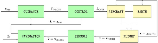
Figure 4. Components of the high-fidelity simulation.

The simulator consists of two distinct processes:

• The first, represented by the yellow blocks on the right of Figure 4, models the physics of flight and the interaction between the aircraft and its surroundings, which results in the real aircraft trajectory ${\displaystyle \mathbf{x}={\mathbf{x}}_{\mathrm{TRUTH}}}$.
• The second, represented by the green blocks on the left, contains the aircraft systems in charge of ensuring that the resulting trajectory adheres as much as possible to the mission objectives. It includes the different sensors whose output comprises the sensed trajectory ${\displaystyle \tilde{\mathbf{x}}={\mathbf{x}}_{\mathrm{SENSED}}}$, the navigation system in charge of filtering it to obtain the estimated trajectory ${\displaystyle \widehat{\mathbf{x}}={\mathbf{x}}_{\mathrm{EST}}}$, the guidance system that converts the reference objectives ${\displaystyle {\mathbf{x}}_{\mathrm{REF}}}$ into the control targets ${\displaystyle {\mathbf{\delta }}_{\mathrm{TARGET}}}$, and the control system that adjusts the position of the throttle and aerodynamic control surfaces ${\displaystyle {\mathbf{\delta }}_{\mathrm{CNTR}}}$ so the estimated trajectory ${\displaystyle \widehat{\mathbf{x}}}$ is as close as possible to the reference objectives ${\displaystyle {\mathbf{x}}_{\mathrm{REF}}}$. Table 1 lists the working frequencies of the various blocks represented in Figure 4.

All components of the flight simulator have been modeled with as few simplifications as much as possible to increase the realism of the results. With the exception of the aircraft performances and its control system, which are deterministic, all other simulator components are treated as stochastic and hence vary from one execution to the next, enhancing the significance of the Monte Carlo simulation results.

Most VIO packages discussed in Section 3 include in their release articles an evaluation when applied to the EuRoC MAV data sets [64], and so do independent evaluations, such as [65]. These data sets contain perfectly synchronized stereo images, IMU measurements, and ground truth readings obtained with laser, for eleven different indoor trajectories flown with a MAV, each with a duration in the order of 2 min and a total distance in the order of ${\displaystyle 100\mathrm{m}}$. This fact by itself indicates that the target application of exiting VIO implementations differs significantly from the main focus of this article, as there may exist accumulating errors that are completely nondiscernible after such short periods of time, but that grow nonlinearly and have the capability of inducing significant pose errors when the aircraft remains aloft for long periods of time. The algorithms presented in this article are hence tested through simulation under two different scenarios designed to analyze the consequences of losing the GNSS signals for long periods of time; these two scenarios coincide with those employed in [1,2] to evaluate standalone visual and inertial algorithms. Most parameters comprising the scenarios are defined stochastically, resulting in different values for every execution. Note that all results shown in Section 10 are based on Monte Carlo simulations comprising one hundred runs of each scenario, testing the sensitivity of the proposed navigation algorithms to a wide variety of values in the parameters.

• Scenario #1 has been defined with the objective of adequately representing the challenges faced by an autonomous fixed-wing UAV that suddenly cannot rely on GNSS and hence changes course to reach a predefined recovery location situated at approximately 1 h of flight time. In the process, in addition to executing an altitude and airspeed adjustment, the autonomous aircraft faces significant weather and wind field changes that make its GNSS-denied navigation even more challenging.
  With respect to the mission, the stochastic parameters include the initial airspeed, pressure altitude, and bearing (${\displaystyle {\mathrm{v}}_{\mathrm{TAS},\mathrm{INI}},{\mathrm{H}}_{\mathrm{P},\mathrm{INI}},{Ø}_{\mathrm{INI}}}$); their final values (${\displaystyle {\mathrm{v}}_{\mathrm{TAS},\mathrm{END}},{\mathrm{H}}_{\mathrm{P},\mathrm{END}},{Ø}_{\mathrm{END}}}$); and the time at which each of the three maneuvers is initiated (turns are executed with a bank angle of ${\displaystyle {\xi }_{\mathrm{TURN}}=\pm {10}^{\circ }}$. Altitude changes employ an aerodynamic path angle of ${\displaystyle {\gamma }_{\mathrm{TAS},\mathrm{CLIMB}}=\pm 2^{\circ }}$. Additionally, airspeed modifications are automatically executed by the control system as set-point changes). The scenario lasts for ${\displaystyle {\mathrm{t}}_{\mathrm{END}}=3800\mathrm{s}}$, while the GNSS signals are lost at ${\displaystyle {\mathrm{t}}_{\mathrm{GNSS}}=100\mathrm{s}}$.
  The wind field is also defined stochastically, as its two parameters (speed and bearing) are constant both at the beginning (${\displaystyle {\mathrm{v}}_{\mathrm{WIND},\mathrm{INI}},{Ø}_{\mathrm{WIND},\mathrm{INI}}}$) and conclusion (${\displaystyle {\mathrm{v}}_{\mathrm{WIND},\mathrm{END}},{Ø}_{\mathrm{WIND},\mathrm{END}}}$) of the scenario, with a linear transition in between. The specific times at which the wind change starts and concludes also vary stochastically among the different simulation runs.
  A similar linear transition occurs with the temperature and pressure offsets that define the atmospheric properties, as they are constant both at the start (${\displaystyle \Delta {\mathrm{T}}_{\mathrm{INI}},\Delta {\mathrm{p}}_{\mathrm{INI}}}$) and end (${\displaystyle \Delta {\mathrm{T}}_{\mathrm{END}},\Delta {\mathrm{p}}_{\mathrm{END}}}$) of the flight.
  The turbulence remains strong throughout the whole scenario, but its specific values also vary stochastically from one execution to the next.
• Scenario #2 represents the challenges involved in continuing with the original mission upon the loss of the GNSS signals, executing a series of continuous turn maneuvers over a relatively short period of time with no atmospheric or wind variations. As in scenario ${\displaystyle \#1}$, the GNSS signals are lost at ${\displaystyle {\mathrm{t}}_{\mathrm{GNSS}}=100\mathrm{s}}$, but the scenario duration is shorter (${\displaystyle {\mathrm{t}}_{\mathrm{END}}=500\mathrm{s}}$). The initial airspeed and pressure altitude (${\displaystyle {\mathrm{v}}_{\mathrm{TAS},\mathrm{INI}},{\mathrm{H}}_{\mathrm{P},\mathrm{INI}}}$) are defined stochastically and do not change throughout the whole scenario; the bearing, however, changes a total of eight times between its initial and final values, with all intermediate bearing values as well as the time for each turn varying stochastically from one execution to the next. Although the same turbulence is employed as in scenario ${\displaystyle \#1}$, the wind and atmospheric parameters (${\displaystyle {\mathrm{v}}_{\mathrm{WIND},\mathrm{INI}},{Ø}_{\mathrm{WIND},\mathrm{INI}},\Delta {\mathrm{T}}_{\mathrm{INI}},\Delta {\mathrm{p}}_{\mathrm{INI}}}$) remain constant throughout scenario ${\displaystyle \#2}$.

10. Results: Navigation System Error in GNSS-Denied Conditions

This section presents the results obtained with the proposed fully integrated visual inertial navigation system when executing Monte Carlo simulations of the two GNSS-denied scenarios introduced in Section 9, each consisting of one hundred executions. They are compared with those obtained with two other navigation systems:

• A standalone inertial system specifically designed to lower the GNSS-denied horizontal position drift, for which the results obtained with the same two scenarios are described in [2]. The attitude estimation error does not drift and is bounded by the quality of the onboard sensors, ensuring that the aircraft can remain aloft for as long as there is fuel available. The vertical position and ground velocity estimation errors are also bounded by atmospheric physics and do not drift; they depend on the atmospheric pressure offset and wind field changes that occur since the GNSS signals are lost. On the other hand, the horizontal position drifts as a consequence of integrating the ground velocity without absolute observations. Note that a standalone inertial system is hence capable of successfully estimating four of the six ${\displaystyle \mathbb{SE}\left(3\right)}$ degrees of freedom (attitude plus altitude).
• A visual navigation system (which relies exclusively on the images generated by an onboard camera) aided by the attitude and altitude estimated by the above inertial system, for which the results are described in [1]. This system slowly drifts in all six degrees of freedom. Although its attitude and altitude estimation capabilities are qualitatively inferior to those of the inertial system, its horizontal position error is just a fraction of what can be achieved without the use of images.

The tables below contain the navigation system error, or NSE (difference between the real states ${\displaystyle \mathbf{x}}$ and their estimations ${\displaystyle \widehat{\mathbf{x}}}$), incurred by the three navigation systems at the conclusion of both scenarios, represented by the mean ${\displaystyle \mu }$, standard deviation ${\displaystyle \sigma }$, and maximum value of the estimation errors. In addition, the figures depict the variation with time of the NSE mean (${\displaystyle \mu }$, solid lines) and standard deviation (${\displaystyle \sigma }$, dashed lines) for the one hundred executions.

10.1. Body Attitude Estimation

Table 3 shows the NSE at the conclusion of the scenarios for the norm of the rotation vector between the real body attitude ${\displaystyle {\mathbf{q}}_{\mathrm{NB}}}$ and its estimation ${\displaystyle {\widehat{\mathbf{q}}}_{\mathrm{NB}}}$, which can be formally written as ${\displaystyle \parallel \Delta {\widehat{\mathbf{r}}}_{\mathrm{NB}}^{\mathrm{B}}\parallel =\parallel {\widehat{\mathbf{q}}}_{\mathrm{NB}}\ominus {\mathbf{q}}_{\mathrm{NB}}\parallel }$. In addition, Figure 5 depicts the variation with time of the body attitude NSE.

Table 3. Aggregated final body attitude NSE (100 runs).

Scenario	${\displaystyle \parallel \mathit{\Delta }{\widehat{\mathbf{r}}}_{\mathbf{NB}}^{\mathrm{B}}\parallel \left({\mathbf{t}}_{\mathbf{END}}\right)\left[{}^{\circ }\right]}$	Inertial	Visual	Proposed
#1	mean	0.158	0.218	0.100
	std	0.114	0.103	0.059
	max	0.611	0.606	0.328
#2	mean	0.128	0.221	0.107
	std	0.078	0.137	0.068
	max	0.369	0.788	0.377

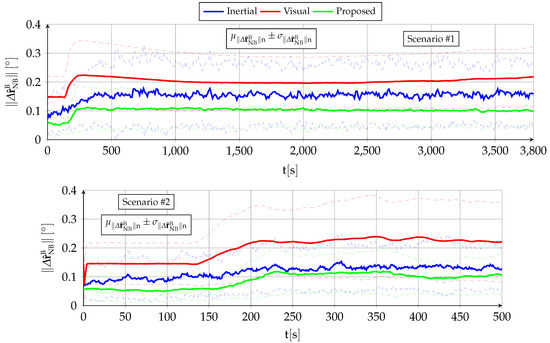
Figure 5. Aggregated body attitude NSE (100 runs).

The proposed visual inertial navigation system shows bounded body attitude estimations, with significant improvements with respect to both the inertial and the inertially assisted visual systems, which can be attributed to various factors. On the one hand, the navigation filter successfully merges the incremental horizontal displacement observations supplied by the VVS with the bearing provided by the magnetometers, resulting in better yaw estimations. In addition, the absence of simplifications in the EKF equations ([2] describes how, without both GNSS receiver and VVS observations, the filter equations need to be simplified to protect the filter behavior from the negative effects of inaccurate velocity and position estimations) ensures that the benefits also reach the already-accurate inertial pitch and bank angle estimations. Additional body attitude estimation improvements are achieved by closing the loop (Figure 2) and directly employing the increasingly accurate inertial estimations to feed the visual system (Section 6).

10.2. Vertical Position Estimation

Table 4 shows the vertical position NSE (${\displaystyle \Delta \widehat{\mathrm{h}}=\widehat{\mathrm{h}}-\mathrm{h}}$) at the conclusion of both scenarios. The estimation errors are unbiased in all cases as the mean is always significantly lower than both the standard deviation and the maximum error value.

Table 4. Aggregated final vertical position NSE (100 runs).

Scenario	${\displaystyle \mathit{\Delta }\widehat{\mathbf{h}}\left({\mathbf{t}}_{\mathbf{END}}\right)\left[\mathbf{m}\right]}$	Inertial	Visual	Proposed
#1	mean	${\displaystyle -}$4.18	+22.86	${\displaystyle -}$3.97
	std	25.78	49.17	26.12
	max	${\displaystyle -}$70.49	+175.76	${\displaystyle -}$70.47
#2	mean	+0.76	+3.59	+0.74
	std	7.55	13.01	7.60
	max	${\displaystyle -}$19.86	+71.64	${\displaystyle -}$18.86

The evolution with time of the geometric altitude NSE is depicted in Figure 6. Note that in contrast with Section 10.1 and Section 10.3, the altitude error is a scalar that can be either positive or negative, so the dashed lines (standard deviation) are more indicative of the relative performance of the various navigation systems, while the solid lines (mean) stay relatively close to zero when averaging the one hundred executions.

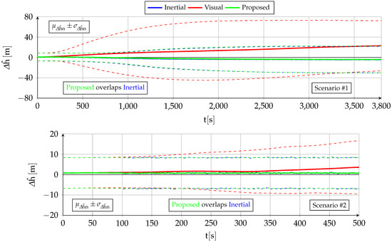
Figure 6. Aggregated vertical position NSE (100 runs).

The vertical position estimation accuracy of the proposed system is virtually the same as that of the standalone inertial one because the navigation filter relies on freezing the pressure offset estimation when the GNSS signals are lost, exactly the same as the inertial filter [2]. The resulting altitude estimations are unbiased and bounded, with an error that depends on the change in pressure offset since the time the GNSS are lost.

10.3. Horizontal Position Estimation

Table 5 lists the mean, standard deviation, and maximum value of the horizontal position NSE at the conclusion of the two scenarios, both in length units and as a percentage of the total distance flown in GNSS-denied conditions. The three navigation systems considered exhibit an unrestrained horizontal position drift or error growth with time, as shown in Figure 7.

Table 5. Aggregated final horizontal position NSE (100 runs).

Scenario			Inertial		Visual		Proposed
		Distance	${\displaystyle \mathit{\Delta }{\widehat{\mathbf{x}}}_{\mathbf{HOR}}\left({\mathbf{t}}_{\mathbf{END}}\right)}$		${\displaystyle \mathit{\Delta }{\widehat{\mathbf{x}}}_{\mathbf{HOR}}\left({\mathbf{t}}_{\mathbf{END}}\right)}$		${\displaystyle \mathit{\Delta }{\widehat{\mathbf{x}}}_{\mathbf{HOR}}\left({\mathbf{t}}_{\mathbf{END}}\right)}$
		${\displaystyle \left[\mathrm{m}\right]}$	${\displaystyle \left[\mathrm{m}\right]}$	${\displaystyle \left[\%\right]}$	${\displaystyle \left[\mathrm{m}\right]}$	${\displaystyle \left[\%\right]}$	${\displaystyle \left[\mathrm{m}\right]}$	${\displaystyle \left[\%\right]}$
#1	mean	107,873	7276	7.10	488	0.46	207	0.19
	std	19,756	4880	5.69	350	0.31	185	0.15
	max	172,842	25,288	32.38	1957	1.48	1257	1.09
#2	mean	14,198	216	1.52	33	0.23	18	0.13
	std	1176	119	0.86	26	0.18	9	0.07
	max	18,253	586	4.38	130	0.98	43	0.33

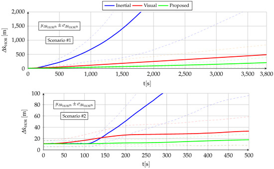
Figure 7. Aggregated horizontal position NSE (100 runs).

The major reduction in horizontal position drift that occurs when comparing the standalone inertial system with the proposed one is obtained in two distinct phases. The first one, described in [1], is caused by employing a visual navigation system that can rely on the inertial attitude and altitude estimations to improve its nonlinear pose optimizations.

The objective when supplying the proposed navigation filter with the VVS observations is to employ more accurate equations within the EKF as there is no longer a need to protect the filter from the negative effects of inaccurate velocity and position values, as in the case of the standalone inertial filter [2]. This improved design enables significant improvements in body attitude accuracy (Section 10.1) because the filter is capable of incorporating the horizontal position accuracy improvements into the EKF filter. In a positive feedback loop, the proposed system then capitalizes on its more accurate attitude estimations to further improve its internal horizontal position estimations (Figure 2).

11. Summary and Conclusions

This article proves that the inertial and visual navigation systems of an autonomous UAV can be combined in such a way that the resulting long-term GNSS-denied horizontal position drift is only a small fraction of what can be achieved by either system individually. The proposed system, however, does not a constitute a full GNSS replacement as it relies on incremental instead of absolute position observations and, hence, can only reduce the position drift but not eliminate it.

The proposed visual inertial navigation filter, specifically designed for the challenges faced by autonomous fixed-wing aircraft that encounter GNSS-denied conditions, merges the observations provided by onboard accelerometers, gyroscopes, and magnetometers with those of the virtual vision sensor, or VVS. The VVS is the denomination of the outputs generated by a visual inertial odometry pipeline that relies on the images of the Earth surface generated by an onboard camera as well as on the navigation filter outputs. The filter is implemented in the manifold of rigid body rotations or ${\displaystyle \mathbb{SO}\left(3\right)}$ in order to minimize the accumulation of errors in the absence of the absolute position observations provided by the GNSS receiver. The results obtained when applying the proposed algorithms to high-fidelity Monte Carlo simulations of two scenarios representative of the challenges of GNSS-denied navigation indicate the following:

• The body attitude estimation is qualitatively similar to that obtained by a standalone inertial filter without any visual aid [2]. The bounded estimations enable the aircraft to remain aloft in GNSS-denied conditions for as long as it has fuel. Quantitatively, the VVS observations and the associated more accurate filter equations result in significant accuracy improvements when compared with the [2] baseline.
• The vertical position estimation is qualitatively and quantitatively similar to that of the standalone inertial filter [2]. In addition to ionospheric effects (which also apply when GNSS signals are available), the altitude error depends on the amount of pressure offset variation since entering GNSS-denied conditions, being unbiased (zero mean) and bounded by atmospheric physics.
• The horizontal position estimation exhibits drastic quantitative improvements over the baseline standalone inertial filter [2], although from a qualitative point of view, the estimation error is not bounded as the drift cannot be fully eliminated.

Future work will focus on addressing some of the limitations of the proposed navigation system, such as the restriction to fixed-wing vehicles (which originates when using the pitot tube airspeed readings to replace visual navigation when not enough features can be extracted from a texture-poor terrain) and the inability to fly at night or above clouds (infrared images could potentially be used for this purpose).

References

- Gallo, E.; Barrientos, A. GNSS-Denied Semi Direct Visual Navigation for Autonomous UAVs Aided by PI-Inspired Priors. Aerospace 2023, 10, 220. [Google Scholar] [CrossRef]
- Gallo, E.; Barrientos, A. Reduction of GNSS-Denied Inertial Navigation Errors for Fixed Wing Autonomous Unmanned Air Vehicles. Aerosp. Sci. Technol. 2021, 120, 107237. [Google Scholar] [CrossRef]
- Sola, J. Quaternion Kinematics for the Error-State Kalman Filter. arXiv 2017, arXiv:1711.02508. [Google Scholar] [CrossRef]
- Sola, J.; Deray, J.; Atchuthan, D. A Micro Lie Theory for State Estimation in Robotics. arXiv 2018, arXiv:1812.01537. [Google Scholar] [CrossRef]
- Gallo, E. The SO(3) and SE(3) Lie Algebras of Rigid Body Rotations and Motions and their Application to Discrete Integration, Gradient Descent Optimization, and State Estimation. arXiv 2023, arXiv:2205.12572. [Google Scholar] [CrossRef]
- Hassanalian, M.; Abdelkefi, A. Classifications, Applications, and Design Challenges of Drones: A Review. Prog. Aerosp. Sci. 2017, 91, 99–131. [Google Scholar] [CrossRef]
- Shakhatreh, H.; Sawalmeh, A.H.; Al-Fuqaha, A.; Dou, Z.; Almaita, E.; Khalil, I.; Othman, N.S.; Khreishah, A.; Guizani, M. Unmanned Aerial Vehicles (UAVs): A Survey on Civil Applications and Key Research Challenges. IEEE Access 2019, 7, 48572–48634. [Google Scholar] [CrossRef]
- Bijjahalli, S.; Sabatini, R.; Gardi, A. Advances in Intelligent and Autonomous Navigation Systems for Small UAS. Prog. Aerosp. Sci. 2020, 115, 100617. [Google Scholar] [CrossRef]
- Farrell, J.A. Aided Navigation, GPS with High Rate Sensors; Electronic Engineering Series; McGraw-Hill: New York, NY, USA, 2008. [Google Scholar]
- Groves, P.D. Principles of GNSS, Inertial, and Multisensor Integrated Navigation Systems; GNSS Technology and Application Series; Artech House: Norwood, MA, USA, 2008. [Google Scholar]
- Chatfield, A.B. Fundamentals of High Accuracy Inertial Navigation; American Institute of Aeronautics and Astronautics, Progress in Astronautics and Aeronautics: Reston, VA, USA, 1997; Volume 174. [Google Scholar]
- Elbanhawi, M.; Mohamed, A.; Clothier, R.; Palmer, J.; Simic, M.; Watkins, S. Enabling Technologies for Autonomous MAV Operations. Prog. Aerosp. Sci. 2017, 91, 27–52. [Google Scholar] [CrossRef]
- Sabatini, R.; Moore, T.; Ramasamy, S. Global Navigation Satellite Systems Performance Analysis and Augmentation Strategies in Aviation. Prog. Aerosp. Sci. 2017, 95, 45–98. [Google Scholar] [CrossRef]
- Tippitt, C.; Schultz, A.; Procino, W. Vehicle Navigation: Autonomy Through GPS-Enabled and GPS-Denied Environments; State of the Art Report DSIAC-2020-1328; Defense Systems Information Analysis Center: Belcamp, MD, USA, 2020. [Google Scholar]
- Gyagenda, N.; Hatilima, J.V.; Roth, H.; Zhmud, V. A Review of GNSS Independent UAV Navigation Techniques. Robot. Auton. Syst. 2022, 152, 104069. [Google Scholar] [CrossRef]
- Kapoor, R.; Ramasamy, S.; Gardi, A.; Sabatini, R. UAV Navigation using Signals of Opportunity in Urban Environments: A Review. Energy Procedia 2017, 110, 377–383. [Google Scholar] [CrossRef]
- Coluccia, A.; Ricciato, F.; Ricci, G. Positioning Based on Signals of Opportunity. IEEE Commun. Lett. 2014, 18, 356–359. [Google Scholar] [CrossRef]
- Goh, S.T.; Abdelkhalik, O.; Zekavat, S.A. A Weighted Measurement Fusion Kalman Filter Implementation for UAV Navigation. Aerosp. Sci. Technol. 2013, 28, 315–323. [Google Scholar] [CrossRef]
- Couturier, A.; Akhloufi, M.A. A Review on Absolute Visual Localization for UAV. Robot. Auton. Syst. 2020, 135, 103666. [Google Scholar] [CrossRef]
- Goforth, H.; Lucey, S. GPS-Denied UAV Localization using Pre Existing Satellite Imagery. In Proceedings of the IEEE International Conference on Robotics and Automation, Montreal, QC, Canada, 20–24 May 2019; IEEE: Piscataway Township, NJ, USA, 2019. [Google Scholar] [CrossRef]
- Ziaei, N. Geolocation of an Aircraft using Image Registration Coupling Modes for Autonomous Navigation. arXiv 2019, arXiv:1909.02875. [Google Scholar] [CrossRef]
- Wang, T. Augmented UAS Navigation in GPS Denied Terrain Environments Using Synthetic Vision. Master’s Thesis, Iowa State University, Ames, IA, USA, 2018. [Google Scholar] [CrossRef]
- Kinnari, J.; Verdoja, F.; Kyrki, V. Season-Invariant GNSS-Denied Visual Localization for UAVs. IEEE Robot. Autom. Lett. 2022, 7, 10232–10239. [Google Scholar] [CrossRef]
- Ren, Y.; Wang, Z. A Novel Scene Matching Algorithm via Deep Learning for Vision-Based UAV Absolute Localization. In Proceedings of the Internaltional Conference on Machine Learning, Cloud Computing and Intelligent Mining, Xiamen, China, 5–7 August 2022. [Google Scholar] [CrossRef]
- Liu, K.; He, X.; Mao, J.; Zhang, L.; Zhou, W.; Qu, H.; Luo, K. Map Aided Visual Inertial Integrated Navigaion for Long Range UAVs. In Proceedings of the Internaltional Conference on Guidance, Navigation, and Control, Sopot, Poland, 12–16 June 2023. [Google Scholar] [CrossRef]
- Zhang, Q.; Zhang, H.; Lan, Z.; Chen, W.; Zhang, Z. A DNN-Based Optical Aided Autonomous Navigation System for UAV Under GNSS-Denied Environment. In Proceedings of the Internaltional Conference on Autonomous Unmanned Systems, Warsaw, Poland, 6–9 June 2023. [Google Scholar] [CrossRef]
- Jurevicius, R.; Marcinkevicius, V.; Seibokas, J. Robust GNSS-Denied Localization for UAV using Particle Filter and Visual Odometry. Mach. Vis. Appl. 2019, 30, 1181–1190. [Google Scholar] [CrossRef]
- Scaramuzza, D.; Fraundorfer, F. Visual Odometry Part 1: The First 30 Years and Fundamentals. IEEE Robot. Autom. Mag. 2011, 18, 80–92. [Google Scholar] [CrossRef]
- Fraundorfer, F.; Scaramuzza, D. Visual Odometry Part 2: Matching, Robustness, Optimization, and Applications. IEEE Robot. Autom. Mag. 2012, 19, 78–90. [Google Scholar] [CrossRef]
- Scaramuzza, D. Tutorial on Visual Odometry; Robotics & Perception Group, University of Zurich: Zurich, Switzerland, 2012. [Google Scholar]
- Scaramuzza, D. Visual Odometry and SLAM: Past, Present, and the Robust Perception Age; Robotics & Perception Group, University of Zurich: Zurich, Switzerland, 2017. [Google Scholar]
- Cadena, C.; Carlone, L.; Carrillo, H.; Latif, Y.; Scaramuzza, D.; Neira, J.; Reid, I.; Leonard, J.J. Past, Present, and Future of Simultaneous Localization and Mapping: Towards the Robust Perception Age. IEEE Trans. Robot. 2016, 32, 1309–1332. [Google Scholar] [CrossRef]
- Forster, C.; Pizzoli, M.; Scaramuzza, D. SVO: Fast Semi-Direct Monocular Visual Odometry. In Proceedings of the IEEE International Conference on Robotics and Automation, Hong Kong, China, 31 May–7 June 2014. [Google Scholar] [CrossRef]
- Forster, C.; Zhang, Z.; Gassner, M.; Werlberger, M.; Scaramuzza, D. SVO: Semidirect Visual Odometry for Monocular and Multicamera Systems. IEEE Trans. Robot. 2016, 33, 249–265. [Google Scholar] [CrossRef]
- Engel, J.; Koltun, V.; Cremers, D. Direct Sparse Odometry. IEEE Trans. Pattern Anal. Mach. Intell. 2018, 40, 611–625. [Google Scholar] [CrossRef]
- Engel, J.; Schops, T.; Cremers, D. LSD-SLAM: Large Scale Direct Monocular SLAM. Eur. Conf. Comput. Vis. 2014, 834–849. [Google Scholar] [CrossRef]
- Mur-Artal, R.; Montiel, J.M.M.; Tardos, J.D. ORB-SLAM: A Versatile and Accurate Monocular SLAM System. IEEE Trans. Robot. 2015, 31, 1147–1163. [Google Scholar] [CrossRef]
- Mur-Artal, R.; Tardos, J.D. ORB-SLAM2: An Open-Source SLAM System for Monocular, Stereo, and RGB-D Cameras. IEEE Trans. Robot. 2017, 33, 1255–1262. [Google Scholar] [CrossRef]
- Mur-Artal, R. Real-Time Accurate Visual SLAM with Place Recognition. Ph.D. Thesis, University of Zaragoza, Zaragoza, Spain, 2017. Available online: http://zaguan.unizar.es/record/60871 (accessed on 25 May 2023).
- Crassidis, J.L.; Markley, F.L. Unscented Filtering for Spacecraft Attitude Estimation. J. Guid. Control Dyn. 2003, 26, 536–542. [Google Scholar] [CrossRef]
- Grip, H.F.; Fossen, T.I.; Johansen, T.A.; Saberi, A. Attitude Estimation Using Biased Gyro and Vector Measurements with Time Varying Reference Vectors. IEEE Trans. Autom. Control 2012, 57, 1332–1338. [Google Scholar] [CrossRef]
- Kottah, R.; Narkhede, P.; Kumar, V.; Karar, V.; Poddar, S. Multiple Model Adaptive Complementary Filter for Attitude Estimation. Aerosp. Sci. Technol. 2017, 69, 574–581. [Google Scholar] [CrossRef]
- Hashim, H.A. Systematic Convergence of Nonlinear Stochastic Estimators on the Special Orthogonal Group SO(3). Int. J. Robust Nonlinear Control 2020, 30, 3848–3870. [Google Scholar] [CrossRef]
- Hashim, H.A.; Brown, L.J.; McIsaac, K. Nonlinear Stochastic Attitude Filters on the Special Orthogonal Group SO(3): Ito and Stratonovich. IEEE Trans. Syst. Man Cybern. 2019, 49, 1853–1865. [Google Scholar] [CrossRef]
- Batista, P.; Silvestre, C.; Oliveira, P. On the Observability of Linear Motion Quantities in Navigation Systems. Syst. Control Lett. 2011, 60, 101–110. [Google Scholar] [CrossRef]
- Hashim, H.A.; Brown, L.J.; McIsaac, K. Nonlinear Pose Filters on the Special Euclidean Group SE(3) with Guaranteed Transient and Steady State Performance. IEEE Trans. Syst. Man Cybern. 2019, 51, 2949–2962. [Google Scholar] [CrossRef]
- Hashim, H.A. GPS Denied Navigation: Attitude, Position, Linear Velocity, and Gravity Estimation with Nonlinear Stochastic Observer. In Proceedings of the 2021 American Control Conference, Online, 25–28 May 2021. [Google Scholar] [CrossRef]
- Hua, M.D.; Allibert, G. Riccati Observer Design for Pose, Linear Velocity, and Gravity Direction Estimation Using Landmark Position and IMU Measurements. In Proceedings of the IEEE Conference on Control Technology and Applications, Copenhagen, Denmark, 21–24 August 2018. [Google Scholar] [CrossRef]
- Barrau, A.; Bonnabel, S. The Invariant Extended Kalman Filter as a Stable Observer. IEEE Trans. Autom. Control 2017, 62, 1797–1812. [Google Scholar] [CrossRef]
- Scaramuzza, D.; Zhang, Z. Visual-Inertial Odometry of Aerial Robots. arXiv 2019, arXiv:1906.03289. [Google Scholar] [CrossRef]
- Huang, G. Visual-Inertial Navigation: A Concise Review. arXiv 2019, arXiv:1906.02650. [Google Scholar] [CrossRef]
- von Stumberg, L.; Usenko, V.; Cremers, D. Chapter 7—A Review and Quantitative Evaluation of Direct Visual Inertial Odometry. In Multimodal Scene Understanding; Yang, M.Y., Rosenhahn, B., Murino, V., Eds.; Academic Press: Cambridge, MA, USA, 2019. [Google Scholar] [CrossRef]
- Feng, X.; Jiang, Y.; Yang, X.; Du, M.; Li, X. Computer Vision Algorithms and Hardware Implementations: A Survey. Integr. Vlsi J. 2019, 69, 309–320. [Google Scholar] [CrossRef]
- Al-Kaff, A.; Martin, D.; Garcia, F.; de la Escalera, A.; Maria, J. Survey of Computer Vision Algorithms and Applications for Unmanned Aerial Vehicles. Expert Syst. Appl. 2017, 92, 447–463. [Google Scholar] [CrossRef]
- Mourikis, A.I.; Roumeliotis, S.I. A Multi-State Constraint Kalman Filter for Vision-aided Inertial Navigation. In Proceedings of the 2007 IEEE International Conference on Robotics and Automation, Roma, Italy, 10–14 April 2007. [Google Scholar] [CrossRef]
- Leutenegger, S.; Furgale, P.; Rabaud, V.; Chli, M.; Konolige, K.; Siegwart, R. Keyframe Based Visual Inertial SLAM Using Nonlinear Optimization. Robot. Sci. Syst. 2013. [Google Scholar] [CrossRef]
- Leutenegger, S.; Lynen, S.; Bosse, M.; Siegwart, R.; Furgale, P. Keyframe Based Visual Inertial SLAM Using Nonlinear Optimization. Int. J. Robot. Res. 2015, 34, 314–334. [Google Scholar] [CrossRef]
- Bloesch, M.; Omari, S.; Hutter, M.; Siegwart, R. Robust Visual Inertial Odometry Using a Direct EKF Based Approach. In Proceedings of the International Conference of Intelligent Robot Systems, Hamburg, Germany, 28 September–3 October 2015. [Google Scholar] [CrossRef]
- Qin, T.; Li, P.; Shen, S. VINS-Mono: A Robust and Versatile Monocular Visual Inertial State Estimator. IEEE Trans. Robot. 2018, 34, 1004–1020. [Google Scholar] [CrossRef]
- Lynen, S.; Achtelik, M.W.; Weiss, S.; Chli, M.; Siegwart, R. A Robust and Modular Multi Sensor Fusion Approach Applied to MAV Navigation. In Proceedings of the International Conference of Intelligent Robot Systems, Tokyo, Japan, 3–7 November 2013. [Google Scholar] [CrossRef]
- Faessler, M.; Fontana, F.; Forster, C.; Mueggler, E.; Pizzoli, M.; Scaramuzza, D. Autonomous, Vision Based Flight and Live Dense 3D Mapping with a Quadrotor Micro Aerial Vehicle. J. Field Robot. 2015, 33, 431–450. [Google Scholar] [CrossRef]
- Forster, C.; Carlone, L.; Dellaert, F.; Scaramuzza, D. On Manifold Pre Integration for Real Time Visual Inertial Odometry. IEEE Trans. Robot. 2017, 33, 1–21. [Google Scholar] [CrossRef]
- Kaess, M.; Johannsson, H.; Roberts, R.; Ila, V.; Leonard, J.; Dellaert, F. iSAM2: Incremental Smoothing and Mapping Using the Bayes Tree. Int. J. Robot. Res. 2012, 31, 216–235. [Google Scholar] [CrossRef]
- Burri, M.; Nikolic, J.; Gohl, P.; Schneider, T.; Rehder, J.; Omari, S.; Achtelik, M.W.; Siegwart, R. The EuRoC MAV Datasets. IEEE Int. J. Robot. Res. 2016, 35, 1157–1163. [Google Scholar] [CrossRef]
- Delmerico, J.; Scaramuzza, D. A Benchmark Comparison of Monocular Visual-Inertial Odometry Algorithms for Flying Robots. In Proceedings of the IEEE International Conference on Robotics and Automation, Brisbane, Australia, 21–25 May 2018. [Google Scholar] [CrossRef]
- Mur-Artal, R.; Montiel, J.M.M. Visual Inertial Monocular SLAM with Map Reuse. IEEE Robot. Autom. Lett. 2017, 2, 796–803. [Google Scholar] [CrossRef]
- Clark, R.; Wang, S.; Wen, H.; Markham, A.; Trigoni, N. VINet: Visual-Inertial Odometry as a Sequence-to-Sequence Learning Problem. In Proceedings of the AAAI Conference on Artificial Intelligence, San Francisco, CA, USA, 4–9 February 2017; Available online: https://ojs.aaai.org/index.php/AAAI/article/view/11215 (accessed on 25 May 2023).
- Paul, M.K.; Wu, K.; Hesch, J.A.; Nerurkar, E.D.; Roumeliotis, S.I. A Comparative Analysis of Tightly Coupled Monocular, Binocular, and Stereo VINS. In Proceedings of the IEEE International Conference on Robotics and Automation, Singapore, 19 May–3 June 2017. [Google Scholar] [CrossRef]
- Song, Y.; Nuske, S.; Scherer, S. A Multi Sensor Fusion MAV State Estimation from Long Range Stereo, IMU, GPS, and Barometric Sensors. Sensors 2017, 17, 11. [Google Scholar] [CrossRef]
- Solin, A.; Cortes, S.; Rahtu, E.; Kannala, J. PIVO: Probabilistic Inertial Visual Odometry for Occlusion Robust Navigation. In Proceedings of the IEEE Winter Conference on Applications of Computer Vision, Lake Tahoe, NV, USA, 12–15 March 2018. [Google Scholar] [CrossRef]
- Houben, S.; Quenzel, J.; Krombach, N.; Behnke, S. Efficient Multi Camera Visual Inertial SLAM for Micro Aerial Vehicles. In Proceedings of the IEEE/RSJ International Conference on Intelligent Robots and Systems, Daejeon, Republic of Korea, 9–14 October 2016. [Google Scholar] [CrossRef]
- Eckenhoff, K.; Geneva, P.; Huang, G. Direct Visual Inertial Navigation with Analytical Preintegration. In Proceedings of the IEEE International Conference on Robotics and Automation, Singapore, 29 May–3 June 2017. [Google Scholar] [CrossRef]
- Negru, S.A.; Geragersian, P.; Petrunin, I.; Zolotas, A.; Grech, R. GNSS/INS/VO Fusion using Gated Recurrent Unit in GNSS-Denied Environments. AIAA SciTech Forum 2023. [Google Scholar] [CrossRef]
- Geragersian, P.; Petrunin, I.; Guo, W.; Grech, R. An INS/GNSS Fusion Architecture in GNSS-Denied Environment using Gated Recurrent Unit. AIAA SciTech Forum 2022. [Google Scholar] [CrossRef]
- Strasdat, H.; Montiel, J.M.M.; Davison, A.J. Real Time Monocular SLAM: Why Filter? In Proceedings of the IEEE International Conference on Robotics and Automation, Anchorage, AK, USA, 3–7 May 2010. [CrossRef]
- Gallego, G.; Delbruck, T.; Orchard, G.; Bartolozzi, C.; Taba, B.; Censi, A.; Leutenegger, S.; Davison, A.; Conradt, J.; Daniilidis, K.; et al. Event Based Cameras: A Survey. IEEE Trans. Pattern Anal. Mach. Intell. 2022, 44, 154–180. [Google Scholar] [CrossRef]
- Mueggler, E.; Gallego, G.; Rebecq, H.; Scaramuzza, D. Continuous Time Visual Inertial Odometry for Event Cameras. IEEE Trans. Robot. 2018, 34, 1425–1440. [Google Scholar] [CrossRef]
- Simon, D. Optimal State Estimation; John Wiley & Sons: Hoboken, NJ, USA, 2006; ISBN 0-471-70858-5. [Google Scholar]
- Blanco, J.L. A Tutorial on SE(3) Transformation Parameterizations and On-Manifold Optimization. arXiv 2020, arXiv:2103.15980. [Google Scholar] [CrossRef]
- Gallo, E. High Fidelity Flight Simulation for an Autonomous Low SWaP Fixed Wing UAV in GNSS-Denied Conditions. C++ Open Source Code. 2020. Available online: https://github.com/edugallogithub/gnssdenied_flight_simulation (accessed on 25 May 2023).
Disclaimer/Publisher’s Note: The statements, opinions and data contained in all publications are solely those of the individual author(s) and contributor(s) and not of MDPI and/or the editor(s). MDPI and/or the editor(s) disclaim responsibility for any injury to people or property resulting from any ideas, methods, instructions or products referred to in the content. |
© 2023 by the authors. Licensee MDPI, Basel, Switzerland. This article is an open access article distributed under the terms and conditions of the Creative Commons Attribution (CC BY) license (https://creativecommons.org/licenses/by/4.0/).