Adaptive IMM-UKF for Airborne Tracking

Abstract

In this paper, we propose a nonlinear tracking solution for maneuvering aerial targets based on an adaptive interacting multiple model (IMM) framework and unscented Kalman filters (UKFs), termed as AIMM-UKF. The purpose is to obtain more accurate estimates, better consistency of the tracker, and more robust prediction during sensor outages. The AIMM-UKF framework provides quick switching between two UKFs by adapting the transition probabilities between modes based on a distance function. Two modes are implemented: a uniform motion model and a maneuvering model. The experimental validation is performed with Monte Carlo simulations of three scenarios with ACAS Xa tracking logic as a benchmark, which is the next generation of airborne collision avoidance systems. The two algorithms are compared using hypothesis testing of the root mean square errors. In addition, we determine the normalized estimation error squared (NEES), a new proposed noise reduction factor to compare the estimation errors against the measurement errors, and an estimated maximum error of the tracker during sensor dropouts. The experimental results illustrate the superior performance of the proposed solution with respect to the tracking accuracy, consistency, and expected maximum error.

1. Introduction

Accurate and robust maneuvering for target tracking is an important research topic as of late in several fields of application, such as air traffic management, air surveillance, collision avoidance, self-driving cars, counter-UAV technologies, and radar tracking. In the military sector, targets are highly maneuverable, and thus traditional tracking algorithms are not suitable. In addition, threats can be stealthy, or their own sensors are under electronic attack. Therefore, coasted tracks due to lack of detection or sensor outages are common.

A variety of solutions have been published on this topic to address maneuverable targets. These solutions can use specific mathematical models for maneuvering targets [1], such as acceleration models (e.g., the white noise acceleration model, Wiener process acceleration model, and Singer acceleration model) or jerk models [2]. Other approaches described in [3] are decision-based, and therefore the logic needs to make a decision about maneuver onset and termination, such as through the adjustable level process noise model, the input estimation filter, or the switching model approach. Other alternatives include those which belong to the multiple model paradigm [4], such as the generalized pseudo-Bayesian (GBP) approach or the interacting multiple model (IMM) filter.

Furthermore, when the model equations are not linear, the Kalman filter cannot be used in the previously described frameworks. Other algorithms such as the extended Kalman filter (EKF), unscented Kalman filter (UKF), or sequential Monte Carlo methods, also known as particle filters, are suitable [5,6]. The latter account for nonlinearity and non-Gaussianity, although they present certifiability issues due to their dependence on random numbers. Another line of research for nonlinear equations has been developed within the theory of differential games as in [7], whose solution is based on feedback control laws.

Recently, the solutions published in the scientific community are an extension of the previous ones, a combination, or based on artificial intelligence (AI). As in [8,9], where an IMM with cubature Kalman filters (CKFs) was designed, the authors of [10] used acceleration and jerk models implemented in an extended Kalman filter (EKF), although this filter is designed for changes in the longitudinal axis. Another approach is that in [11], which suggests an IMM-UKF model composed of three filters with the same dynamic model but different noise covariances and a gray neural network to predict the position errors. The authors of [12] used three models with different dynamics—the constant velocity (CV), adaptive current statistical model (CS), and the constant speed rate constant steering rate model—and it adapts the parameters of the CS model. The authors of [13] adapted the maximum acceleration, which was not fixed, as it is in the traditional current statistical model. The authors of [14] introduced fuzzy logic to update the model probabilities of the IMM. The authors of [15] proposed an adaptive sampling policy, in which the sampling rate increases during the maneuver mode. The authors of [16] adapted the transition matrix according to the sampling period.

The AI-based methods usually introduce a neural network with memory ability to extract features from the data sequence. Usually, two techniques are used. The first one is to use a neural network to carry out a specific and bounded task to maintain the explainability of the model, such as KalmanNet [17], where a neural network is designed to compute the Kalman gain with a gate recurrent unit (GRU), or the method from the authors of [18], who defined deep learning maneuvering and target tracking based on the long short-term memory (LSTM) network. The second technique uses a deep learning model to perform all the tracking tasks from feature extraction from the observation sequence to state estimation based on those features, as in [19], where a Transformer-based network (TBN) was used, or in [20] with Bi-LSTM networks.

Regarding the performance analysis of the tracking logic, typically, these papers use some simulations to measure the estimation errors via the root mean square errors (RMSEs), as stated in [21]. Some papers compare several tracking algorithms by comparing the RMS estimation errors under the same conditions. This is the standard, such as in [11,12,22,23], where the maximum estimation errors are also analyzed. Other papers analyze the absolute errors, such as [24], where four nonlinear filters for ballistic target tracking are compared. However, there is no comparison between the proposed tracking logic and algorithms from other research papers since, with the current analysis, this is not possible. The reason for this is that the estimation errors are dependent on the measurement errors, and thus they should be analyzed against them as shown in Section 3. To the best of the author’s knowledge, there are no research works in the literature in which the noise reduction factor metric is determined.

In addition, we have identified that most tracking algorithms do not consider the transient state when switching between different modes. Therefore, we propose a novel algorithm to improve the performance when tracking maneuvering targets. The purpose of this work is therefore twofold: to present a new metric that takes into consideration the measurement errors and enable tracking performance comparisons and to propose a new algorithm that considers the transient state for aircraft tracking.

The rest of this paper is structured as follows. In the next section, we detail the proposed tracking algorithm. Then, in Section 3, we explain the Monte Carlo simulation framework used to verify the airborne tracking logic. Section 4 presents the selected scenarios and the results of the experimental validation. Finally, a conclusion is presented in Section 5.

2. Tracking Logic

This section outlines the material used in this research, focusing on the tracking logic without addressing the measurement origin uncertainty. Therefore, this paper addresses the single maneuvering target tracking problem. We propose a novel adaptive IMM-UKF algorithm, which is compared against a benchmark. We selected the Cartesian tracker of the next generation of airborne collision avoidance systems (ACAS Xa) as the state of the art of airborne target tracking.

First, we provide a brief description of ACAS Xa. In 2018, the Federal Aviation Administration (FAA) published the Minimum Operational Performance Standard (MOPS) of ACAS Xa [25], which details that the surveillance tracking module (STM) is composed of three trackers:

• A Cartesian tracker to estimate the horizontal coordinates and velocity of an aircraft relative to the ownship by means of an augmented UKF;
• A range tracker to estimate the horizontal range and the relative horizontal speed by means of a UKF as well;
• A vertical tracker to estimate the vertical position and velocity of an othership aircraft using a Kalman filter.

The estimation algorithms used in ACAS Xa for these three trackers are not coupled. This means that the dependency between the estimation results of each one is only due to dependencies in the measurement data inputs of the three filters. The selected benchmark was the Cartesian tracker, which was specified in [26]. It makes use of an augmented UKF in combination with a Mahalanobis distance-based outlier detection logic. The aircraft evolution model used within the UKF is uniform linear motion. This means that it is assumed that the relative trajectory follows the constant velocity model. The measurement model is based on a secondary surveillance radar, which provides the slant range, bearing, and altitude measurements. Note that aside from secondary surveillance radar, ACAS Xa supports hybrid surveillance through the use of ADS-B in order to reduce radar interrogations. But hybrid surveillance is only used when the intruder is not a near threat. In addition, ADS-B measurements are processed by a different tracker: the ADS-B tracker, which implements a Kalman filter. Consequently, the measurement model used is based on the radar equations.

The stochastic difference equation of motion adopted by the Cartesian tracker is shown in Equation (1):

$${\left(\begin{array}{c}x\\ y\\ v_x\\ v_y\end{array}\right)}_{k+1}\left[\begin{array}{cccc}1& 0& dt& 0\\ 0& 1& 0& dt\\ 0& 0& 1& 0\\ 0& 0& 0& 1\end{array}\right]·{\left(\begin{array}{c}x\\ y\\ v_x\\ v_y\end{array}\right)}_k+\left[\begin{array}{cc}0.5d{t}^2& 0\\ 0& 0.5d{t}^2\\ dt& 0\\ 0& dt\end{array}\right]·v\left(k\right).$$

(1)

where v(k) is a series of random variables that are independent and identically distributed, with zero mean and a variance $Q=512f{t}^2/s^4$.

The Cartesian tracker adopted measurement equations at moment k are for the slant range $r_k$ and bearings ${\theta }_k$, shown in Equations (2) and (3):

$$r_k=\sqrt{x^2+y^2}+n_r\left(k\right).$$

(2)

$${\theta }_k=atan(y/x)+n_{\theta }\left(k\right).$$

(3)

The measurement noises are assumed to be independent and identically distributed, with zero mean and variances $R_r=2500$ ft${}^2$ and $R_{\theta }=0.030461742$ rad${}^2$.

On the other hand, the proposed algorithm is an adaptive interacting multiple model (AIMM) based on the original IMM depicted in [27]. This filter considers the trajectory of the aircraft as a stochastic hybrid system.

If the trajectory of the target is considered the usual stochastic system, then the state variables are the position and velocity, and it is assumed that the state meets the Markov property. However, in stochastic hybrid systems theory, this is not true, and the state is extended with a discrete value called the mode, which indicates the dynamics of the target. Therefore, it is the mathematical model which better adapts to the target’s motion. Under this assumption, the trajectory changes due to the mode switching (discrete process) and the evolution of the continuous process demonstrated in [28,29], and that is the reason why it is called a hybrid process. The IMM combines multiple models, each representing a different dynamic behavior. The system switches between these models to adapt to the changing dynamics of the aircraft being tracked. The adaptive IMM provides adaptive capabilities to the model selection process. In our proposed adaptive IMM, the method to influence the model selection is to adapt the transition probability matrix based on the residuals of each model, specifically the Mahalanobis distance, when the measurement residuals of a model increase and the transition probability to stay in that model is reduced.

The first step of the IMM is mixing, which combines the estimates obtained from the individual models (r) to generate a fused or mixed estimate of the state of the system ${\widehat{x}}^{0j}$ (Equation (5)) and the covariance $P^{0j}$ (Equation (6)). The weights are called the mixing probabilities ${\mu }_{i|j}$ (Equation (4)). Note that mixing is one of the most important steps, since it is one of the main differences with respect to other suboptimal multiple model estimators [30]:

$${\mu }_{i|j}=p_{ij}·{\mu }_i/(\sum _{i=1}^r{p}_{ij}·{\mu }_i),$$

(4)

$${\widehat{x}}^{0j}=\sum _{i=1}^r{\widehat{x}}^i·{\mu }_{i|j},$$

(5)

$$P^{0j}=\sum _{i=1}^r[{\mu }_{i|j}·[P^i+({\widehat{x}}^i-{\widehat{x}}^{0j})·{({\widehat{x}}^i-{\widehat{x}}^{0j})}^T]],$$

(6)

where $p_{ij}$ is the transition probability from mode i to mode j and ${\mu }_i$ is the probability of being in mode i.

Given that there are two modes, the transition probability matrix $\mathsf{\Pi }$ (Equation (7)), whose elements ${\mu }_{i|j}$ express the probability of switching from one mode to another, is a square matrix of the size 2 × 2 with the following initial values:

$$\mathsf{\Pi }=\left(\begin{array}{cc}0.95& 0.1\\ 0.05& 0.9\end{array}\right)$$

(7)

Secondly, in the mode-matched filtering step, where the filter of each mode is executed, the IMM discrete value mode is composed of two models:

• Mode 1 or non-maneuvering mode: in uniform linear motion, this mode is modeled with the same equations previously described.
• Mode 2 or maneuvering mode: the coordinated turn model [31], also known as the constant speed constant turn rate (CSCTR) model, which supports right and left turns. Its implementation is based on Equation (8) with the coordinated turn equations and multi-dimensional Brownian motion v(k).

The process equation of the coordinated turn model (Equation (8)) is used to determine the prediction based on the previous estimate:

$$\begin{array}{c}\hfill {\left(\begin{array}{c}x\\ y\\ v_x\\ v_y\\ \omega \end{array}\right)}_{k+1}=\left[\begin{array}{ccccc}1& 0& {\displaystyle \frac{sin\left(\omega T\right)}{\omega }}& -{\displaystyle \frac{1-cos\left(\omega T\right)}{\omega }}& 0\\ 0& 1& {\displaystyle \frac{1-cos\left(\omega T\right)}{\omega }}& {\displaystyle \frac{sin\left(\omega T\right)}{\omega }}& 0\\ 0& 0& cos\left(\omega T\right)& -sin(\omega T& 0\\ 0& 0& sin\left(\omega T\right)& cos\left(\omega T\right)& 0\\ 0& 0& 0& 0& 1\end{array}\right]·{\left(\begin{array}{c}x\\ y\\ v_x\\ v_y\\ \omega \end{array}\right)}_k+\left[\begin{array}{ccc}0.5d{t}^2& 0& 0\\ 0& 0.5d{t}^2& 0\\ dt& 0& 0\\ 0& dt& 0\\ 0& 0& dt\end{array}\right]·v\left(k\right).\end{array}$$

(8)

Each mode filter uses the unscented Kalman filter and thus is composed of a prediction update cycle, which is depicted with the typical state space representation: the process (Equation (9)) and the measurement equation (Equation (10)):

$$x_k=f(x_{k-1},w_{k-1}),$$

(9)

$$z_k=h(x_k,v_k),$$

(10)

The prediction in the UKF uses the unscented transform to determine the resulting distribution of passing a Gaussian distribution through the nonlinear prediction equation. The unscented transform uses a set of sigma points 2n + 1, (Equations (11) and (12)) and its corresponding weights (Equations (13) and (14)):

$${\chi }^{\left(0\right)}={\widehat{x}}_t$$

(11)

$${\chi }^{\left(i\right)}={\widehat{x}}_t\pm \left(\sqrt{(n+\lambda )·{\widehat{P}}_t}\right),$$

(12)

$$w^{\left(0\right)}={\displaystyle \frac{\lambda }{n+\lambda }},$$

(13)

$$w^{\left(i\right)}={\displaystyle \frac{1}{2·(n+\lambda )}},$$

(14)

where n is the dimensionality of the system and $\lambda$ is a scaling factor that influences the spread of the sigma points.

Latterly, the sigma points are predicted, and the resulting distribution is approximated by a Gaussian distribution with the mean and covariance specified in Equations (15) and (16):

$$x_{t_k+1}^{\prime }=\sum _{i=0}^{2n}{w}^{\left(i\right)}·f\left({\chi }^{\left(i\right)}\right)$$

(15)

$$P_{t_k+1}^{\prime }=\sum _{i=0}^{2n}{w}^{\left(i\right)}·(f\left({\chi }^{\left(i\right)}\right)-x_{t_k+1}^{\prime })·{(f\left({\chi }^{\left(i\right)}\right)-x_{t_k+1}^{\prime })}^T+Q$$

(16)

Next, the predicted sigma points are transformed into the measurement space (Equation (17)), and the distribution is characterized with the predicted measurement mean (Equation (18)) and covariance (Equation (19)):

$$Z^{\left(i\right)}=h\left({\chi }^{\left(i\right)}\right)$$

(17)

$$z^{\prime }=\sum _{i=0}^{2n}{w}^{\left(i\right)}·Z^{\left(i\right)}$$

(18)

$$S=\sum _{i=0}^{2n}{w}^{\left(i\right)}·(Z^{\left(i\right)}-z^{\prime })·{(Z^{\left(i\right)}-z^{\prime })}^T+R$$

(19)

Then, during the update step, the predicted state and covariance are updated (Equations (22) and (23)) with the Kalman gain K (Equation (20)) and the innovation (Equation (21)):

$$K=[\sum _{i=0}^{2n}{w}^{\left(i\right)}·({\chi }^{\left(i\right)}-x_{t_k+1}^{\prime })·{(Z^{\left(i\right)}-z^{\prime })}^T]·S^{-1}$$

(20)

$$\nu =z-z^{\prime }$$

(21)

$${\widehat{x}}_{t_k+1}^i=x_{t_k+1}^i·K·{\nu }_{t_k+1}^i$$

(22)

$${\widehat{P}}_{t_k+1}^i=(I-K·T)·P_{t_k+1}^i$$

(23)

Later, during the mode probability update, the likelihood ${\mathsf{\Lambda }}_j$ of each model is computed (Equation (24)) in order to estimate the probability mode ${\mu }_j$ (Equation (25)). The likelihood of each model expresses the degree of belief in how well the observed data align with each model:

$${\mathsf{\Lambda }}_j=\mathit{N}(z_j\left(k\right);{\widehat{z}}_j\left(k\right|k-1),S_j\left(k\right|k-1))$$

(24)

$${\mu }_j=1/c·{\mathsf{\Lambda }}_j·\sum _{i=1}^r{p}_{ij}·{\mu }_i$$

(25)

where $z_j\left(k\right)$ is the measurement, ${\widehat{z}}_j\left(k\right|k-1)$ is the predicted measurement of the filter j, $S_j\left(k\right|k-1)$ is the innovation covariance of the filter j, and c is the normalization constant.

One of the problems with relying only on the computed likelihoods to determine the mode probabilities arises in highly uncertain scenarios. When the innovation covariance is too big, the mode likelihoods from Equation (24) will not vary a lot from each other since the Gaussian distribution of the innovation is too broad, and thus the IMM filter needs time to converge to the proper mode. To overcome this limitation, an adaptive technique is proposed. This adaptive method allows one to adjust the model probabilities more quickly than the traditional IMM. The main difference is that the IMM only modifies the mode probabilities based on the likelihoods. The proposed AIMM defines a primary and secondary mode based on a distance function, thereby easing the transition toward the primary mode and better adapting to the measurements. This adaptive feature allows the algorithm to better handle the transient periods where the system dynamics change, whereas the IMM does not address this issue.

Subsequently, the adaptation method of the proposed AIMM consists of modifying the transition probability matrix based on a distance function between the measurement and the predicted measurement (Equation (26)), specifically the Mahalanobis distance $d_M$, since it allows us to compute the distance between two distributions. When the Mahalanobis distance of the uniform motion model increases over a threshold (in this case, 15% over the Mahalanobis distance of the coordinated turn model), then the columns of the transition probability matrix are exchanged to ease the transition to the other mode:

$$d_M=\sqrt{{({\widehat{z}}_j\left(k\right|k-1)-z_j\left(k\right))}^T·S^{-1}·({\widehat{z}}_j\left(k\right|k-1)-z_j\left(k\right))}$$

(26)

Finally, the estimation and covariance of each mode are combined based on the minimum mean square error estimator, and the previously computed mode probabilities (Equations (27) and (28)) are consequently considered:

$${\widehat{x}}_{t_k+1}=\sum _{i=1}^r{\widehat{x}}^i·{\mu }_i,$$

(27)

$${\widehat{P}}_{t_k+1}=\sum _{i=1}^r[{\mu }_i·[P^i+({\widehat{x}}^i-\widehat{x})·{({\widehat{x}}^i-\widehat{x})}^T]],$$

(28)

3. Monte Carlo Method

This section defines the research method. Given that we are dealing with stochastic difference equations, the selected research method is Monte Carlo simulation. The Monte Carlo simulator is based on the Collision Avoidance Validation and Evaluation Tool (CAVEAT) simulator presented in [32], and its specifications below ensure the replicability of this study. Note that the CAVEAT simulator can be requested at the Eurocontrol website.

The aircraft evolution and measurement equations used for the simulation are detailed further in [33,34]. Regarding noise models, there are several approaches in the literature, such as the one proposed in [35], where the slant range and bearing errors are modeled with zero-mean Gaussian distributions, or the method proposed in [36], which is a time-correlated Gaussian error model.

The transponder-based slant range noise model used is depicted below (Equation (29)):

$$r_t^{measured}=r_t^{true}+{ϵ}^{r,bias}+{ϵ}^{r,jitter}.$$

(29)

The slant range error ${ϵ}^r$ is modeled with a constant bias and a variable jitter component. The parameter values are those corresponding to mode S of transponder signaling, as stated in [4]. The bias is a series of independent and identically distributed random variables from a normal distribution, with zero as the mean and a standard deviation equal to 125 ft (Equation (30)):

$${ϵ}^{r,bias}\sim f^N(.;0,125ft).$$

(30)

And the jitter component is described with a first-order autoregressive model (Equation (31)) with Gaussian white noise and a standard deviation equal to 50 ft (Equation (32)):

$${ϵ}_t^{r,jitter}={\alpha }^{auto,r}·{ϵ}_{t-1}^{r,jitter}+{ϵ}_t^{noise}.$$

(31)

$${ϵ}_t^{noise}\sim f^N(.;0,{\sigma }^{r,jitter}·\sqrt{1-{\alpha }^{auto,r2}}).$$

(32)

The transponder-based bearing noise model is depicted below (Equation (33)):

$${\theta }_t^{measured}={\theta }_t^{true}+{ϵ}_t^{r,jitter}\left(\vartheta \right).$$

(33)

The relative bearing error is modeled only with a jitter component, which is well described with a first-order autoregressive model with Gaussian white noise and a standard deviation equal to 10°.

The metrics for analyzing the performance of the estimation logic are as follows:

• The RMS errors in each of the state variables (x, y, $v_x$, $v_y$). This is the most popular type of error in tracking for measuring accuracy because it is sensitive to outliers (i.e., it penalizes large estimation errors more heavily due to the squared differences).
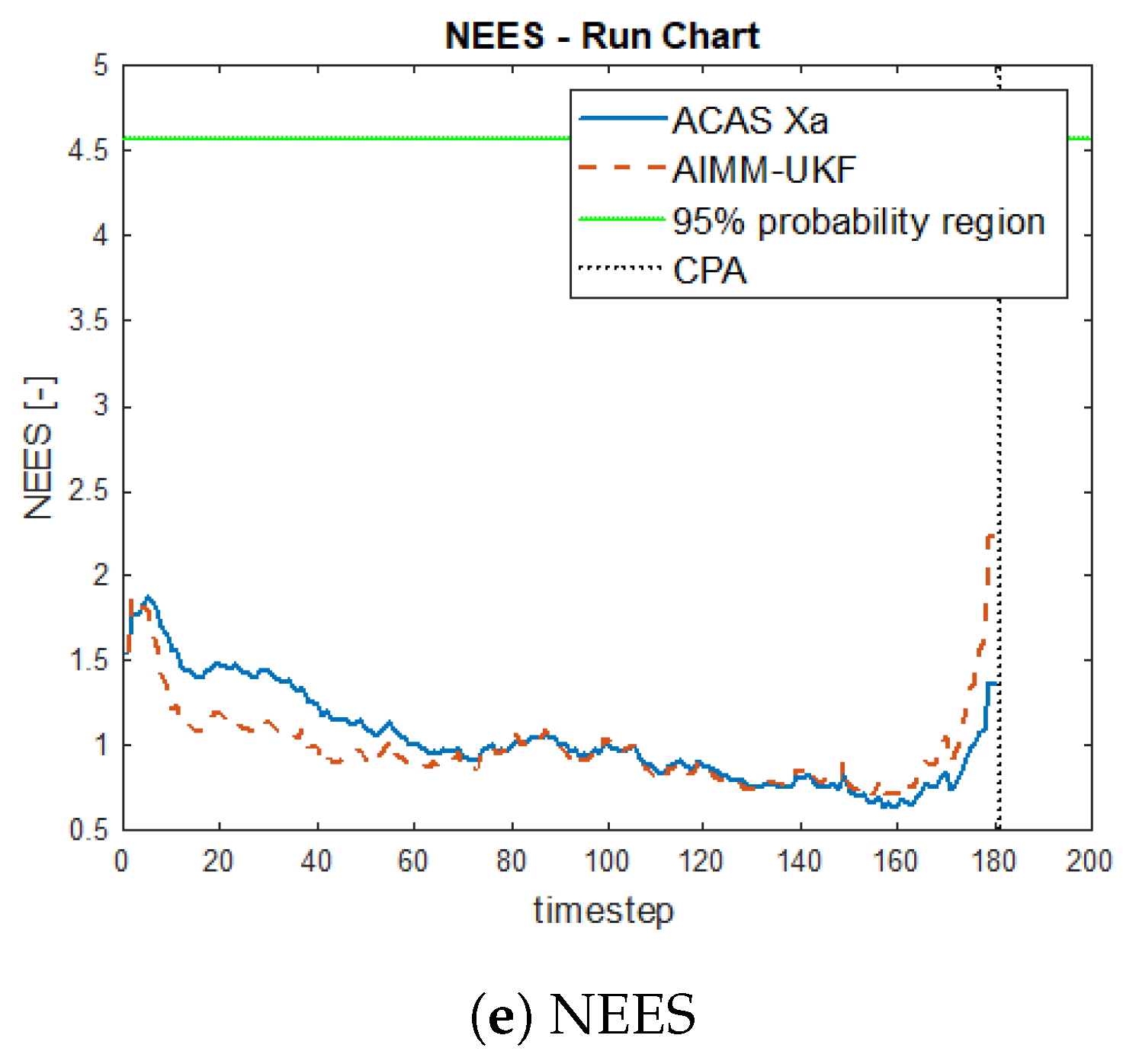
• The normalized estimation error squared (NEES) error and its 95% probability region for checking the consistency of the filter, as stated in [21]. The consistency analysis studies whether the output covariance matrix corresponds or not to the provided state. If the estimation error is much greater than its corresponding covariance, then the filter is overconfident; otherwise, it is underconfident. This is the preferred metric when the ground truth is available due to its easy interpretation and normalization.
• The settling time against velocity changes to measure the tracker’s lag. This is useful for assessing the velocity of adaptation in dynamic systems during transient periods.
• The noise reduction factor provided by the tracker. This is accomplished by assessing the difference between the measurement error (tracker´s input) and the estimation error (tracker´s output), and it shows how much noise is filtered out by the tracking logic.

The latter is not the standard used in other papers (e.g., [11,12]). This enables performance comparison between different trackers under different conditions.

Neither metric should be used individually. They should be used in conjunction with other evaluation metrics to find a comprehensive understanding of the performance: accuracy, consistency, velocity of adaptation, and filtering performance.

According to the central limit theorem, the mean errors from an infinite number of MC runs will follow a Gaussian distribution. Because the number of MC runs is finite, this Gaussian assumption does not need to apply. Nevertheless, we assume Gaussianity in order to obtain a ratio distribution that can be approximated to a normal distribution, as explained in [37].

The number of Monte Carlo runs was selected to be 2000 runs, which was based on the desired margin of error of 20 ft in the position confidence intervals and to ensure that the central limit theorem applied.

4. Experiments and Results

Three encounters between the ownship and an othership aircraft were selected to evaluate the tracking logic performance. These encounters were selected to have a variety of relative trajectories (linear and curvilinear):

• Uniform linear motion applied for both aircraft;
• The ownship aircraft behaved in uniform linear motion, while the othership aircraft made a turn;
• This encounter simulates a relative trajectory with a step function as the velocity.

Note that encounters 1 and 2 are representative of true aircraft behavior, since they were based on the Collision Avoidance Fast-Time Evaluator (CAFE) tool [38], which generates encounters by learning the features from true encounters.

At the end, the sensor outages were analyzed.

4.1. Encounter 1

In the first encounter, both aircraft had uniform linear motion (Figure 1), and the relative trajectory was also linear (Figure 2). Figure 3 and Figure 4 and

Table 1. Summary table of the results for encounter 1.

Variable	Mean	Median	Std Dev	75th Percentile	25th Percentile
ACAS Xa-RMSE x (ft)	426	281.3	457	573.7	121
ACAS Xa-RMSE y (ft)	724.1	464.6	853.4	973.7	180.8
ACAS Xa-RMSE $v_x$ (ft/s)	33.17	13.1	61.3	25.8	5.9
ACAS Xa-RMSE $v_y$ (ft/s)	35.7	25	34.4	47.3	11.4
IMM-RMSE x (ft)	390.9	265.5	417.3	528	115.9
IMM-RMSE y (ft)	749.4	490.2	862.5	1021.4	189.9
IMM-RMSE $v_x$ (ft/s)	33.5	16	56.9	30.2	14.1
IMM-RMSE $v_y$ (ft/s)	41.5	31.2	36.5	57.8	14.2
Measured RMSE x (ft)	906.2	904.2	63.6	949	860.1
Measured RMSE y (ft)	2145.5	2137.8	143	2241.7	2051

provide the MC simulation results.

The root mean square errors of the state variables are represented in Figure 3a–e. Note that in the run charts, the RMS errors were analyzed until the moment of closest point of approach (CPA).

Regarding the NEES run chart in Figure 3e, the 95% probability region was plotted in order to assess the consistency of the filter, and as we can see in the graph, the filter was consistent in this encounter.

Finally, the distributions of the measurement error and the estimation error are compared in Figure 4a,b for the x and y coordinates. The mean of the noise reduction factor was 0.47 and 0.43 for the x coordinate and 0.34 and 0.35 for the y coordinate for ACAS Xa and the IMM, respectively.

The results data from the MC simulations can be seen in Table 1:

4.2. Encounter 2

In the second encounter (Figure 5), aircraft 1 had uniform linear motion, and aircraft 2 was turning counter-clockwise. As a result, the relative trajectory was curvilinear (Figure 6). Figure 7 and Figure 8 and

Table 2. Summary table of the results for encounter 2.

Variable	Mean	Median	Std Dev	75th Percentile	25th Percentile
ACAS Xa-RMSE x (ft)	2515	2001	2195	3407	1017
ACAS Xa-RMSE y (ft)	1783	1470	1655	2362	736
ACAS Xa-RMSE $v_x$ (ft/s)	187.6	135.8	159.2	279.6	66.3
ACAS Xa-RMSE $v_y$ (ft/s)	121.5	92.9	112	157	44
IMM-RMSE x (ft)	2182	1700	2049	2817	866.8
IMM-RMSE y (ft)	1698	1390	1600	2277	677.7
IMM-RMSE $v_x$ (ft/s)	153.7	113.5	146.4	186.1	58.7
IMM-RMSE $v_y$ (ft/s)	122.2	83.4	107.6	166	46
Measured RMSE x (ft)	5628	5618	321	5837	5415
Measured RMSE y (ft)	4568	4561	262	4741	4380

provide the MC simulation results.

The RMS errors of the state variables are represented in the following run charts (Figure 7). The RMSE errors were greater than those in encounter 1, since the geometry of the encounter was more demanding and therefore more difficult to model.

Regarding the NEES run chart in Figure 7e, the 95% probability region is plotted in order to assess the consistency of the filter. As we can see in the graph, the adaptive IMM logic presented greater consistency even when the target was maneuvering, whereas the benchmark was not consistent in this encounter when the target was maneuvering, since the NEES error exceeded the 95% probability region. Consequently, the adaptive techniques provided better adaptations to nonlinear trajectories.

Finally, the distributions of the measurement error and estimation error are compared in Figure 8a,b. The mean of the noise reduction factor was 0.43 and 0.38 for the x coordinate and 0.39 and 0.36 for the y coordinate for ACAS Xa and the IMM, respectively.

The result data from the MC simulations can be seen in Table 2:

4.3. Encounter 3

In this encounter, aircraft 2 was in uniform linear motion, and aircraft 1 started with uniform linear motion but suddenly changed direction as a holonomic agent. The result was that the relative velocity followed a step function in terms of both speed and direction. The speed changed from an initial value of 480 Kts to a final value of 339 Kts, and the direction changed from −135 degrees to −90 degrees (Figure 9). The purpose of this was to measure the reactivity to changes in velocity by determining the settling time.

The reaction to velocity changes was studied from two perspectives: its direction in Figure 9b and its speed in Figure 9a. The settling time of the speed (i.e., the time required for the estimated speed to become steady within a range of 5% of its final value) was similar for ACAS Xa and the IMM. However, the settling time for the direction was 23 s and 73 s for the IMM and ACAS Xa, respectively.

4.4. Estimation Error Analysis

Finally, a hypothesis test was performed to compare the performance of ACAS Xa and the AIMM-UKF in encounters 1 and 2. Given that the purpose of the Cartesian tracker is to estimate the horizontal miss distance (HMD), we applied the two-sample t-test for this variable. In order to apply this hypothesis test, we needed to first test for normality. A Kolmogorov–Smirnov test was used for this purpose, where the null hypothesis was that the data from each encounter came from a normal distribution. As a result of the test, the data could be considered normal.

The next step was to compute the two-sample t-test, where the null hypothesis was that the data from the two samples (ACAS Xa and AIMM-UKF) came from independent random samples from normal distributions with equal means and variances. For the first encounter (rectilinear trajectory), the null hypothesis was not rejected, see

Table 3. Hypothesis test for ACAS Xa and IMM RMSE HMD.

Encounter	Hypothesis Test	p-Value	Outcome
Encounter 1	Two-sample t-test	0.18	Not rejected
Encounter 2	Two-sample t-test	6.8 × 10−60	Rejected

. Therefore, we could not conclude that one algorithm performed better. However, for the second encounter (curvilinear), the error in the horizontal position was different depending on the algorithm used. The IMM performed better, as we can see in the confidence interval graph in Figure 10a,b.

Note that the hypothesis test was performed by comparing the algorithms within the same scenario because the geometries of the scenarios were so different that if we compared the tracking logic in the two scenarios, we would see that the performance in encounter 1 was greater than that in encounter 2, as we can see if we compare the confidence intervals in Figure 10a,b.

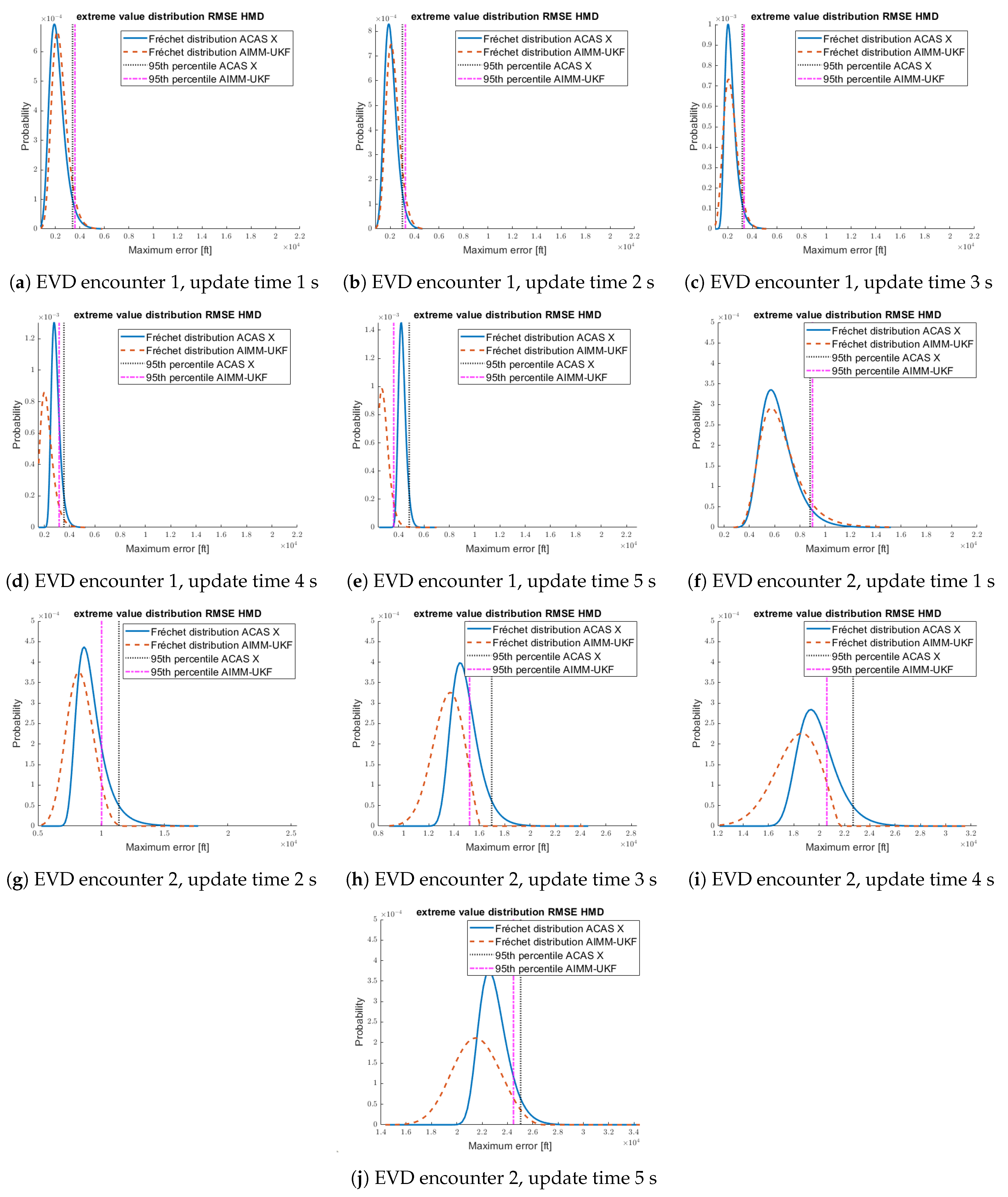
4.5. Robustness of the Prediction

Moreover, an analysis of the maximum expected error during sensor outages is also interesting for measuring the robustness of the filter. As we can see in Figure 10a,b, the errors in encounter 2 were greater than those in encounter 1 due to the nonlinearities of the encounter. In this section, we try to analyze the maximum error of the tracker. It seems fair to think that if the motion model and the true trajectory diverge, then the coasted tracks (i.e., those tracks which are predicted without updates) will have the maximum error. One of the causes of coasted tracks is sensor outages due to sensor malfunction or electronic attack. For this purpose, we estimated the maximum expected error using extreme value distribution and Monte Carlo simulation with different update time values for the tracking logic and different encounters. We tested from 1 s to 5 s every 1 s, and as we can see, the block maxima of the estimation errors followed the generalized extreme value distribution, specifically the Fréchet distribution (Figure 11).

A comparison between the maximum expected error in the previous scenarios is interesting. As seen in Figure 12, the maximum error increased when the update time increased, but the effect was more severe when the trajectory was highly nonlinear and when the prediction model did not consider nonlinear trajectories. On the other hand, for the same update time, the maximum error was greater in the nonlinear trajectory.

5. Conclusions

A new adaptive interacting multiple model was designed and compared to the current state of the art for airborne target tracking: the ACAS Xa estimation logic. Both algorithms were analyzed for three encounters with different geometries. These encounters were carefully selected in order to analyze the different dynamics of the system of interest, which was the relative trajectory of the othership aircraft with respect to the ownship. The simulation results’ analysis showed that the adaptive multiple model-based tracking logic had better performance than the single model-based logic with respect to the estimation accuracy, consistency, and robustness of the prediction. The main reason for this is that modeling the trajectory as a stochastic hybrid system better adapts to the nature of a maneuvering target.

In the first encounter, the trajectory of the aircraft was aligned with the process equation of uniform motion. Therefore, both filters were consistent, and there was no significant difference between ACAS Xa and the AIMM-UKF.

In encounter 2, the RMS errors of the state variables were greater than those in encounter 1. The reason for obtaining a different behavior in the second encounter was that in the second encounter, the relative trajectory did not follow a uniform linear motion since it was a curvilinear trajectory. Therefore, the performance of the estimation logic decreased, and we can see that the single-mode tracking algorithms were not consistent, while the adaptive IMM performed better. Consequently, the AIMM-UKF reduced its dependency on the encounter´s geometry.

This limitation related to the motion model and the encounter’s geometry was shown to worsen when the update time of the Kalman logic increased due to sensor outages. As shown by the extreme value distributions, the maximum error increased linearly, although the gradient was slower for the adaptive IMM, which showed greater robustness.

A third encounter was selected to stress the logic with a sudden and abrupt maneuver and measure the settling time of the velocity. It was shown that the AIMM-UKF provided quick adaptation to the maneuver, since the velocity settling time was shown to be lower.

Aside from that, the estimation errors, which depend on the measurement errors perceived by the system and on the performance of the filter (how much noise is able to filter out), and the measurement errors were compared to assess the performance of the tracking logic. The AIMM-UKF performed better, yielding a noise reduction factor between 0.36 and 0.43. This information is useful for future research, since other tracking logics could be compared against these tracking algorithms while taking into account the dependency on the measurement noise.

These research results will benefit the design of target tracking systems, especially in counter-UAV technologies or military applications, where the targets are highly maneuverable. In the future, the generation of a dataset of airspace encounters with ground truth data and observation data will benefit the research in aircraft tracking. In addition, the introduction of modern artificial intelligence methods in the proposed framework will be investigated in a future study.

References

1. Li, X.R.; Jilkov, V.P. Survey of Maneuvering Target Tracking. Part I. Dynamic Models. IEEE Trans. Aerosp. Electron. Syst. 2003, 39, 1333–1364. [Google Scholar] [CrossRef]
2. Mahapatra, P.R.; Mehrotra, K. Mixed Coordinate Tracking of Generalized Maneuvering Targets using acceleration and Jerk Models. IEEE Trans. Aerosp. Electron. Syst. 2000, 36, 992–1000. [Google Scholar] [CrossRef] [Green Version]
3. Li, X.R.; Jilkov, V.P. A Survey of Maneuvering Target Tracking: Decision-Based Methods. Proc. SPIE Conf. Signal Data Process. Small Targets 2002, 4728, 511–534. [Google Scholar] [CrossRef]
4. Li, X.R.; Jilkov, V.P. Survey of Maneuvering Target Tracking. Part V. Multiple-Model Methods. IEEE Trans. Aerosp. Electron. Syst. 2005, 41, 1255–1321. [Google Scholar] [CrossRef]
5. Li, L.-Q.; Xie, W.-X.; Huang, J.-X.; Huang, J.-J. Multiple Model Rao-Blackwellized Particle Filter for Manoeuvring Target Tracking. Def. Sci. J. 2009, 59, 197–204. [Google Scholar] [CrossRef] [Green Version]
6. Foo, P.H.; Ng, G.W. Combining the Interacting Multiple Model Method with Particle Filters for Manoeuvring Target Tracking. IET Radar Sonar Navig. 2011, 5, 234–255. [Google Scholar] [CrossRef]
7. Osipov, Y.S.; Maksimov, V.I. Tracking the Solution to a Nonlinear Distributed Differential Equation by Feedback Laws. Numer. Anal. Appl. 2018, 11, 158–169. [Google Scholar] [CrossRef]
8. Liu, H.; Wu, W. Interacting Multiple Model (IMM) Fifth-Degree Spherical Simplex-Radial Cubature Kalman Filter for Maneuvering Target Tracking. Sensors 2017, 17, 1374. [Google Scholar] [CrossRef] [PubMed] [Green Version]
9. Han, B.; Huang, H.; Lei, L.; Huang, C.; Zhang, Z. An improved IMM algorithm Based on STSRCKF for Maneuvering Target Tracking. IEEE Access 2019, 7, 57795–57804. [Google Scholar] [CrossRef]
10. Ghosh, S.; Mukhopadhyay, S. Tracking Reentry Ballistic Targets using Acceleration and Jerk Models. IEEE Trans. Aerosp. Electron. Syst. 2011, 47, 666–683. [Google Scholar] [CrossRef]
11. Xu, Q.; Li, X.; Chan, C.Y. A Cost-Effective Vehicle Localization Solution Using and Interacting Multiple Model Unscented Kalman Filters (IMM-UKF) Algorithm and Grey Neural Network. Sensors 2017, 17, 1431. [Google Scholar] [CrossRef] [Green Version]
12. Zhiwen, H.; Fanliang, B. A small UAV tracking algorithm based on AIMM-UKF. Aircr. Eng. Aerosp. Technol. 2021, 93, 579–592. [Google Scholar]
13. Ding, Z.; Liu, Y.; Liu, J.; Yu, K.; You, Y.; Jing, P.; He, Y. Adaptive Interacting Multiple Model Algorithm Based on Information-Weighted Consensus for Maneuvering Target Tracking. Sensors 2018, 18, 2012. [Google Scholar] [CrossRef] [PubMed] [Green Version]
14. Guo, Q.; Teng, L. Maneuvering Target Tracking with Multi-Model Based on the Adaptive Structure. IEEJ Trans. Electr. Electron. Eng. 2022, 17, 865–871. [Google Scholar] [CrossRef]
15. Puranik, S.P.; Tugnait, J.K. On Adaptive sampling for Multisensor Tracking of a Maneuvering Target using IMM/PDA filtering. In Proceedings of the 2005 American Control Conference, Portland, OR, USA, 8–10 June 2005. [Google Scholar] [CrossRef]
16. Kim, W.C.; Musicki, D.; Song, T.L. Adaptive Mode Transition Matrix for Variable Sampling Time, In Proceedings of the 17th International Conference on Information Fusion, Salamanca, Spain, 7–10 July 2014; IEEE: Piscataway, NJ, USA, 2014.
17. Revach, G.; Shlezinger, N.; Ni, X.; Lopez, A.; van Sloun, R.J.G.; Eldar, Y.C. KalmanNet: Neural Network Aided Kalman Filtering for Partially Known Dynamics. IEEE Trans. Signal Process. 2022, 70, 1532–1547. [Google Scholar] [CrossRef]
18. Liu, J.; Wang, Z.; Xu, M. DeepMTT: A Deep Learning Maneuvering Target Tracking Algorithm Based on Bidirectional LSTM network. Inf. Fusion 2020, 53, 289–304. [Google Scholar] [CrossRef]
19. Zao, G.; Wang, Z.; Huang, Y.; Zhang, H.; Ma, X. Transformer-Based Maneuvering Target Tracking. Sensors 2022, 22, 8482. [Google Scholar] [CrossRef]
20. Tian, W.; Fang, L.; Li, W.; Ni, N.; Wang, R.; Hu, C.; Liu, H.; Luo, W. Deep-Learning-Based Multiple Model Tracking Method for Targets with Complex Maneuvering Motion. Remote Sens. 2022, 14, 3276. [Google Scholar] [CrossRef]
21. Bar Shalom, Y.; Li, X.R.; Kirubarajan, T. Estimation with Applications to Tracking and Navigation; Wiley: Hoboken, NJ, USA, 2001. [Google Scholar]
22. Schubert, R.; Richter, E.; Wanielik, G. Comparison and Evaluation of Advanced Motion Models for Vehicle Tracking. In Proceedings of the 11th International Conference on Information Fusion IEEE, Cologne, Germany, 30 June–3 July 2008; pp. 1–6. [Google Scholar]
23. Li, L.Q.; Xie, W.X. Bearings-only maneuvering target tracking based on fuzzy clustering in a cluttered environment. Int. J. Electron. Commun. 2014, 68, 130–137. [Google Scholar]
24. Farina, A.; Ristic, B.; Benvenutti, D. Tracking a Ballistic Target: Comparison of several non linear filters. Trans. Aerosp. Electron. Syst. 2002, 38, 854–867. [Google Scholar] [CrossRef]
25. RTCA. Minimum Operational Performance Standards for Airborne Collision Avoidance System X (ACAS X); RTCA: Washington, CA, USA, 2019. [Google Scholar]
26. EUROCAE. MOPS for ACAS Xa with ACAS Xo Functionality, Volume II; EUROCAE: Saint-Denis, France, 2018. [Google Scholar]
27. Blom, H.A.P.; Bar-Shalom, Y. The Interacting Multiple Model Algorithm For Systems with Markovian Switching Coefficents. IEEE Trans. Autom. Control 1988, 33, 780–783. [Google Scholar] [CrossRef]
28. Blom, H.A.P. An Efficient Decision-Making-Free Filter For Processes With Abrupt Changes. IFAC Proc. Vol. 1985, 18, 631–636. [Google Scholar] [CrossRef]
29. Blom, H.A.P. Overlooked Potential of Systems with Markovian Coefficients. In Proceedings of the IEEE Conference on Decision and Control, Athens, Greece, 10–12 December 1986; pp. 1758–1764. [Google Scholar]
30. Bar-Shalom, Y.; Challa, S.; Blom, H.A.P. IMM Estimator versus Optimal Estimator for Hybrid Systems. IEEE Trans. Aerosp. Electron. Syst. 2005, 41, 986–991. [Google Scholar] [CrossRef]
31. Blackman, S.S.; Popoli, R.F. Design and Analysis of Modern Tracking Systems; Artech House: Norwood, MA, USA, 1999; p. 1232. [Google Scholar]
32. Stroeve, S.; Blom, H.; Hernandez Medel, C.; Garcia Daroca, C.; Arroyo Cebeira, A.; Drozdowski, S. Development of a Collision Avoidance Validation and Evaluation Tool (CAVEAT): Adressing the intrinsic uncertainty in TCAS II and ACAS X. In Proceedings of the 13th USA/Europe Air Traffic Management Research and Development Seminar, Vienna, Austria, 17–21 June 2019. [Google Scholar]
33. Stroeve, S.; Blom, H.A.; Canizares, C.V.; Ba, G.J. CAVEAT Phase 2 Models and Algorithms, Development of a Collision Avoidance Validation and Evaluation Tool, Report NLR-CR-2018-429; NLR: Amsterdam, The Netherlands, 2020. [Google Scholar]
34. Stroeve, S.; Blom, H.A.; Hernandez Medel, C.; Garcia Daroca, C.; Arroyo Cebeira, A.; Drozdowski, S. Modeling and Simulation of Intrinsic Uncertainties in Validation of Collision Avoidance Systems. J. Air Transp. AIAA 2020, 28, 173–183. [Google Scholar] [CrossRef]
35. Chryssanthacopolos, P.; Kochenderfer, M.J. Accounting for State Uncertainty in Collision Avoidance. J. Guid. Control Dyn. 2011, 34, 951–960. [Google Scholar] [CrossRef]
36. Panken, A.D.; Kochenderfer, M.J. Error Model Estimation for Airborne Beacon-based. IET Radar Sonar Navig. 2014, 8, 667–675. [Google Scholar] [CrossRef]
37. Hayya, J.; Armstrong, D.; Gressis, N. A Note on the Ratio of Two Normally Distributed Variables. Manag. Sci. 1975, 56, 635–639. [Google Scholar] [CrossRef] [Green Version]
38. Eurocontrol. SESAR PJ.13-Solution 111 Description of Collision Avoidance Fast-Time Evaluator (CAFE) Revised Encounter Model for Europe (CREME) (Report No. D2.1.090). Available online: https://skybrary.aero/sites/default/files/bookshelf/33312.pdf (accessed on 20 June 2023).
Figure 1. Plan view of encounter 1.
Aerospace 10 00698 g001
Figure 2. Relative trajectory of encounter 1.
Aerospace 10 00698 g002
Figure 3. Run chart of the RMS errors.
Aerospace 10 00698 g003aAerospace 10 00698 g003b
Figure 4. Measurement and estimation RMSE comparison. (a) RMS error comparison for the x coordinate. (b) RMS error comparison for the y coordinate.
Aerospace 10 00698 g004
Figure 5. Plan view of encounter 2.
Aerospace 10 00698 g005
Figure 6. Relative trajectory encounter 2.
Aerospace 10 00698 g006
Figure 7. Run chart of the RMS errors in encounter 2.
Aerospace 10 00698 g007
Figure 8. Measurement and estimation RMSE X comparison.
Aerospace 10 00698 g008
Figure 9. Tracker response to speed step function.
Aerospace 10 00698 g009
Figure 10. Confidence interval RMSE HMD.
Aerospace 10 00698 g010
Figure 11. Extreme value distributions (EVDs).
Aerospace 10 00698 g011
Figure 12. Maximum error behavior.
Aerospace 10 00698 g012