
A Data-Light and Trajectory-Based Machine Learning Approach for the Online Prediction of Flight Time of Arrival


Abstract
1. Introduction
1.1. Literature Review
1.2. Contributions of the Paper
1.3. Organization of the Paper
2. Methodology
2.1. Definition
2.2. Overall Framework for ETA_TAB and ELDT Prediction
2.3. Trajectory Point Reconstruction and Matching
2.3.1. Trajectory Point Reconstruction
2.3.2. Trajectory Matching
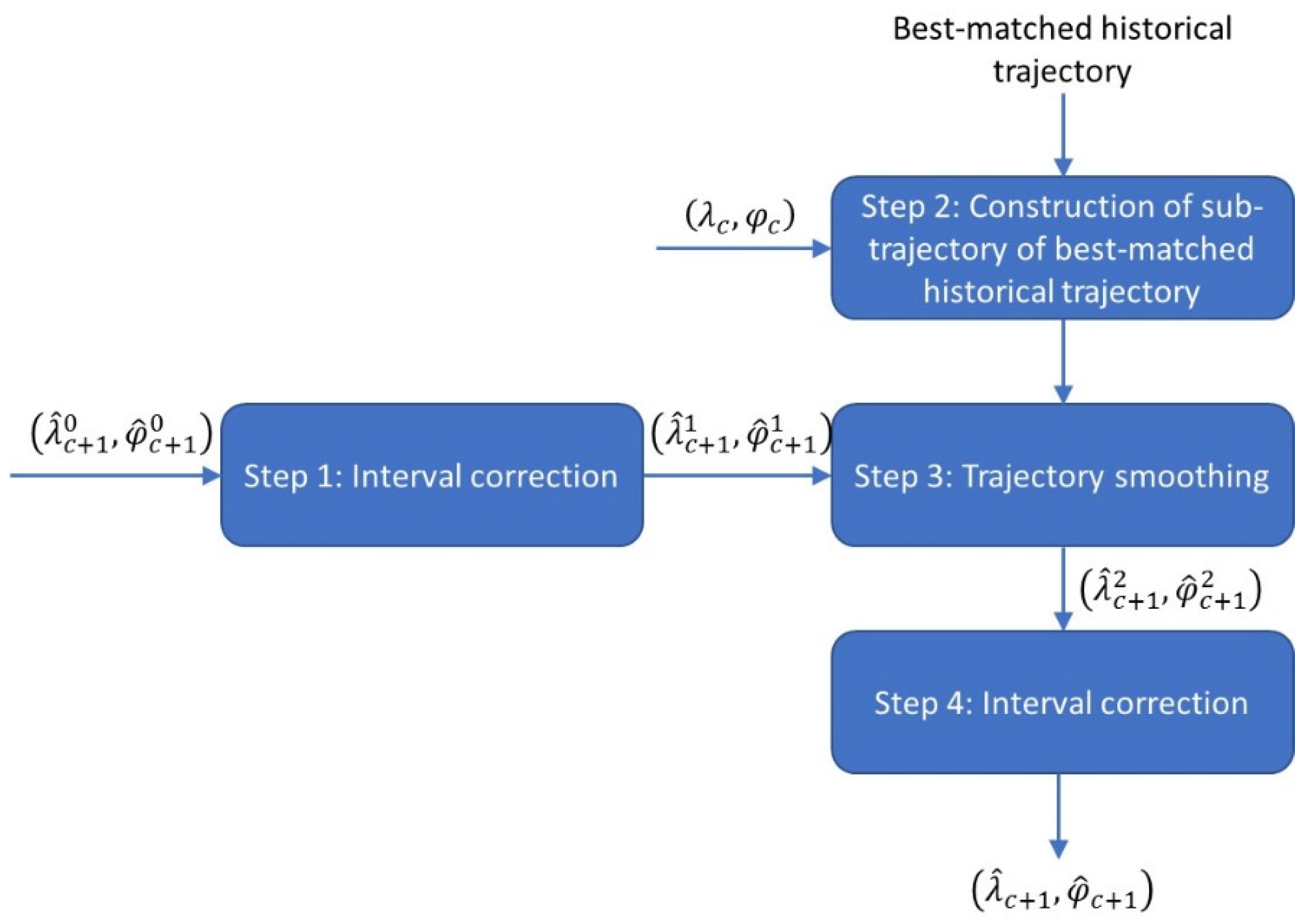
2.4. Trajectory Prediction
2.4.1. LSTM Neural Network
2.4.2. LSTM Network for Trajectory Prediction
2.5. Ground Speed Prediction
| Algorithm1: GBM Algorithm | |
| 1. | |
| 2. | do: |
| 3. | |
| 4. | |
| 5. | |
| 6. | End for |
2.6. ETA_TAB and ELDT Prediction
3. Demonstration of the Prediction Approach
3.1. Data
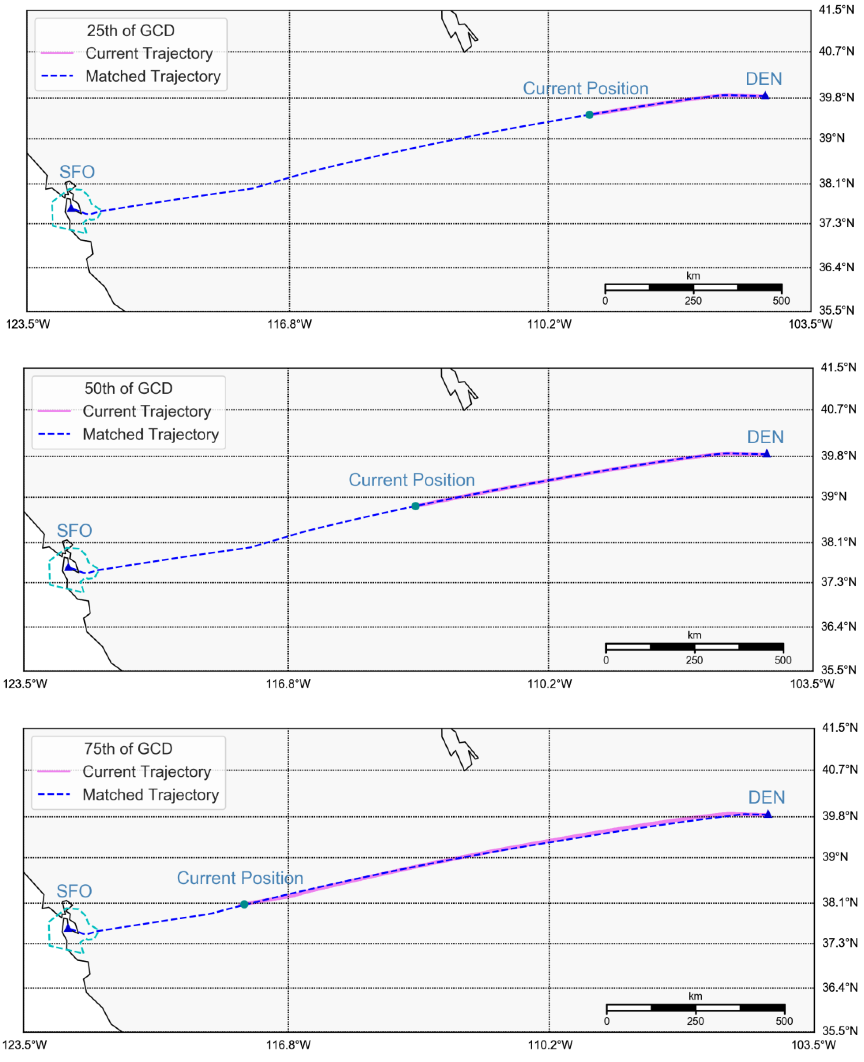
3.2. Trajectory Matching
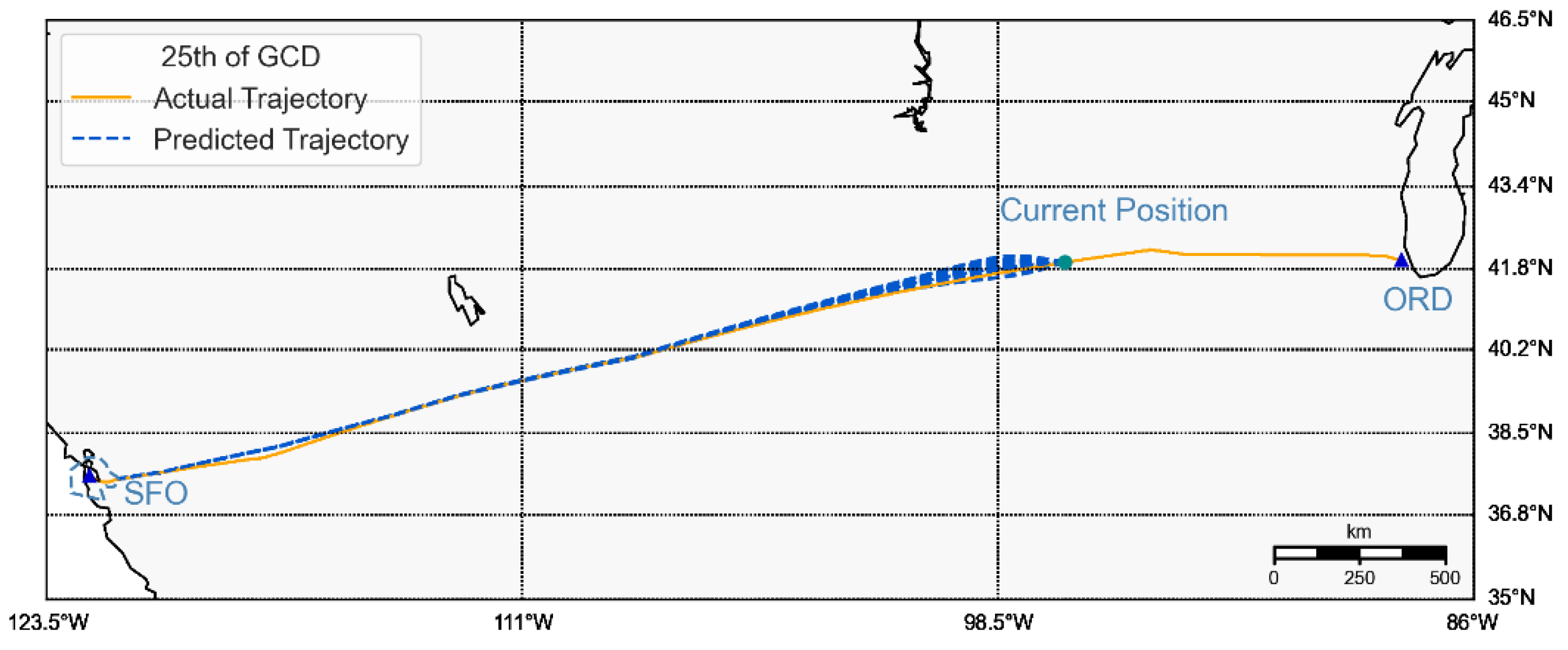
3.3. Trajectory Prediction
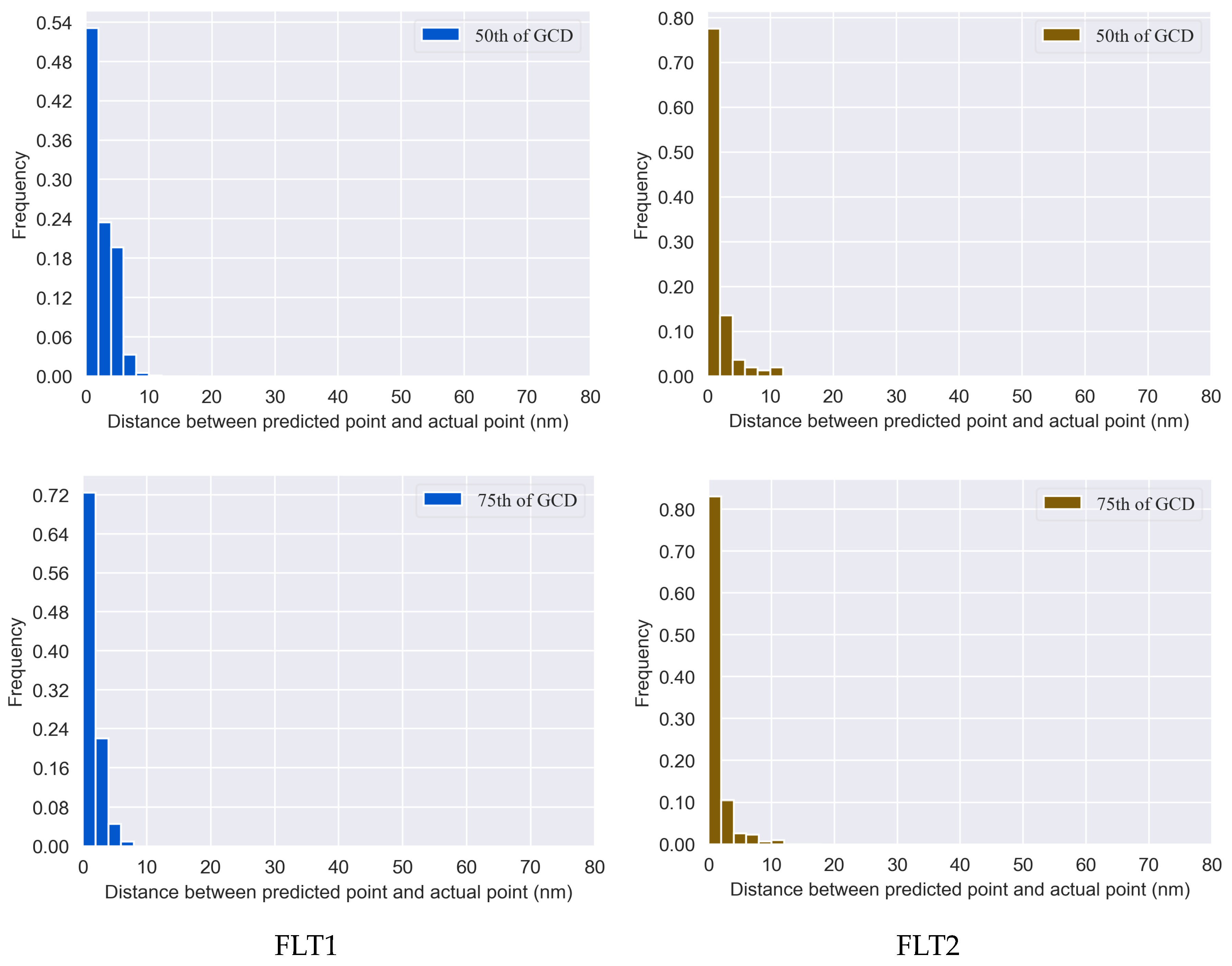
3.4. Ground Speed Prediction
3.5. ETA_TAB and ELDT Prediction
3.5.1. ETA_TAB Prediction
3.5.2. ELDT Prediction
Sampling Terminal Approach Time
Results
4. Summary and Further Discussion
Author Contributions
Funding
Data Availability Statement
Conflicts of Interest
Appendix A. Ground Speeds of FLT1 and FLT2

References
- Heere, K.R.; Zelenska, R.E. A Comparison of Center/TRACON Automation System and Airline Time of Arrival Predictions. No. NAS 1.15: 209584; National Aeronautics and Space Administration, Ames Research Center: Moffett Field, CA, USA, 2000. [Google Scholar]
- Huang, H.; Roy, K.; Tomlin, C. Probabilistic Estimation of State-Dependent Hybrid Mode Transitions for Aircraft Arrival Time Prediction. In Proceedings of the AIAA Guidance, Navigation and Control Conference and Exhibit, Hilton Head, CA, USA, 20–23 August 2007; p. 6695. [Google Scholar]
- Flightradar24. Using the New FLIGHTRADAR24 KML and CSV Export Tools. 2020. Available online: https://www.flightradar24.com/blog/using-the-new-flightradar24-kml-and-csv-export-tools/ (accessed on 25 August 2020).
- Hochreiter, S.; Schmidhuber, J. Long short-term memory. Neural Comput. 1997, 9, 1735–1780. [Google Scholar] [CrossRef] [PubMed]
- Graves, A.; Jaitly, N. Towards end-to-end speech recognition with recurrent neural networks. In Proceedings of the 31st International Conference on Machine Learning (ICML-14), Beijing, China, 21–26 June 2014; pp. 1764–1772. [Google Scholar]
- Chorowski, J.; Bahdanau, D.; Cho, K.; Bengio, Y. End-to-end continuous speech recognition using attention-based recurrent NN: First results. arXiv 2014, arXiv:1412.1602. [Google Scholar]
- Chung, J.; Kastner, K.; Dinh, L.; Goel, K.; Courville, A.C.; Bengio, Y. A recurrent latent variable model for sequential data. In Advances in Neural Information Processing Systems 28; Curran Associates Inc.: Red Hook, NY, USA, 2015; pp. 2980–2988. [Google Scholar]
- Sutskever, I.V. Sequence to sequence learning with neural networks. In Advances in Neural Information Processing Systems 27; Curran Associates Inc.: Red Hook, NY, USA, 2014; pp. 3104–3112. [Google Scholar]
- Karpathy, A.; Fei-Fei, L. Deep visual-semantic alignments for generating image descriptions. In Proceedings of the IEEE Conference on Computer Vision and Pattern Recognition, Boston, MA, USA, 7–12 June 2015; pp. 3128–3137. [Google Scholar]
- Vinyals, O.; Toshev, A.; Bengio, S.; Erhan, D. Show and tell: Lessons learned from the 2015 mscoco image captioning challenge. IEEE Trans. Pattern Anal. Mach. Intell. 2016, 39, 652–663. [Google Scholar] [CrossRef] [PubMed]
- Friedman, J.H. Greedy function approximation: A gradient boosting machine. Ann. Stat. 2001, 29, 1189–1232. [Google Scholar]
- Ma, X.; Ding, C.; Luan, S.; Wang, Y.; Wang, Y. Prioritizing influential factors for freeway incident clearance time prediction using the gradient boosting decision trees method. IEEE Trans. Intell. Transp. Syst. 2017, 18, 2303–2310. [Google Scholar] [CrossRef]
- Ding, C.; Cao, X.J.; Næss, P. Applying gradient boosting decision trees to examine non-linear effects of the built environment on driving distance in Oslo. Transp. Res. Part A Policy Pract. 2018, 110, 7–117. [Google Scholar] [CrossRef]
- Barua, L.; Zou, B.; Liu, Y. Modeling Household Online Shopping Demand in the US: A Machine Learning Approach and Comparative Investigation between 2009 and 2017. arXiv 2021, arXiv:2101.03690. [Google Scholar]
- Barua, L.; Zou, B. Planning maintenance and rehabilitation activities for airport pavements: A combined supervised machine learning and reinforcement learning approach. Int. J. Transp. Sci. Technol. 2022, 11, 423–435. [Google Scholar] [CrossRef]
- Krozel, J.L. Estimating time of arrival in heavy weather conditions. In Proceedings of the AIAA Guidance, Navigation, and Control Conference and Exhibit, Portland, OR, USA, 9–11 August 1999; p. 4232. [Google Scholar]
- Bai, X.; Weitz, L.A.; Priess, S. Evaluating the impact of estimated time of arrival accuracy on interval management performance. In Proceedings of the AIAA Guidance, Navigation, and Control Conference, San Diego, CA, USA, 4–8 January 2016; p. 1852. [Google Scholar]
- Franco, A.; Rivas, D.; Valenzuela, A. Probabilistic aircraft trajectory prediction in cruise flight considering ensemble wind forecasts. Aerosp. Sci. Technol. 2018, 82, 350–362. [Google Scholar] [CrossRef]
- Zhang, J.; Liu, J.; Hu, R.; Zhu, H. Online four dimensional trajectory prediction method based on aircraft intent updating. Aerosp. Sci. Technol. 2018, 77, 774–787. [Google Scholar] [CrossRef]
- Shi, Z.; Xu, M.; Pan, Q. 4-D Flight trajectory prediction with constrained LSTM network. IEEE Trans. Intell. Transp. Syst. 2020, 22, 7242–7255. [Google Scholar] [CrossRef]
- Ayhan, S.; Costas, P.; Samet, H. Predicting estimated time of arrival for commercial flights. In Proceedings of the 24th ACM SIGKDD International Conference on Knowledge Discovery & Data Mining, London, UK, 19–23 August 2018; pp. 33–42. [Google Scholar]
- De Leege, A.; van Paassen, M.; Mulder, M. A machine learning approach to trajectory prediction. In Proceedings of the AIAA Guidance, Navigation, and Control (GNC) Conference, Boston, MA, USA, 19–22 August 2013; p. 4782. [Google Scholar]
- Wang, Z.; Liang, M.; Delahaye, D. A hybrid machine learning model for short-term estimated time of arrival prediction in terminal manoeuvring area. Transp. Res. Part C Emerg. Technol. 2018, 95, 280–294. [Google Scholar] [CrossRef]
- Wang, Z.; Liang, M.; Delahaye, D. Automated data-driven prediction on aircraft Estimated Time of Arrival. J. Air Transp. Manag. 2020, 88, 101840. [Google Scholar] [CrossRef]
- Glina, Y.; Jordan, R.; Ishutkina, M. A tree-based ensemble method for the prediction and uncertainty quantification of aircraft landing times. In Proceedings of the American Meteorological Society–10th Conference on Artificial Intelligence Applications to Environmental Science, New Orleans, LA, USA, 22–26 January 2012. [Google Scholar]
- Kim, M.S. Analysis of short-term forecasting for flight arrival time. J. Air Transp. Manag. 2016, 52, 35–41. [Google Scholar] [CrossRef]
- Achenbach, A.; Spinler, S. Prescriptive analytics in airline operations: Arrival time prediction and cost index optimization for short-haul flights. Oper. Res. Perspect. 2018, 5, 265–279. [Google Scholar] [CrossRef]
- Lui, G.N.; Klein, T.; Liem, R.P. Data-Driven Approach for Aircraft Arrival Flow Investigation at Terminal Maneuvering Area. In Proceedings of the AIAA AVIATION 2020 Forum, Online, 15–19 June 2020; p. 2869. [Google Scholar]
- Liu, Y.; Hansen, M. Predicting aircraft trajectories: A deep generative convolutional recurrent neural networks approach. arXiv 2018, arXiv:1812.11670. [Google Scholar]
- Zhang, X.; Mahadevan, S. Bayesian neural networks for flight trajectory prediction and safety assessment. Decis. Support Syst. 2020, 131, 113246. [Google Scholar] [CrossRef]
- Shi, Z.; Xu, M.; Pan, Q.; Yan, B.; Zhang, H. LSTM-based flight trajectory prediction. In Proceedings of the 2018 International Joint Conference on Neural Networks (IJCNN), Rio de Janeiro, Brazil, 8–13 July 2018; pp. 1–8. [Google Scholar]
- OpenFlight. Retrieved from Airport, Airline and Route Data. Available online: https://openflights.org/data.html (accessed on 15 May 2022).
- Olah, C. Understanding LSTM Networks. Available online: https://colah.github.io/posts/2015-08-Understanding-LSTMs/ (accessed on 22 January 2021).
- Movable Type Ltd. Calculate Distance, Bearing and more between Latitude/Longitude Points. Available online: https://www.movable-type.co.uk/scripts/latlong.html (accessed on 26 August 2020).
- Hastie, T.; Tibshirani, R.; Friedman, J. The Elements of Statistical Learning; Springer: New York, NY, USA, 2009. [Google Scholar]
- Murça, M.C.R.; Hansman, R.J.; Li, L.; Ren, P. Flight trajectory data analytics for characterization of air traffic flows: A comparative analysis of terminal area operations between New York, Hong Kong and Sao Paulo. Transp. Res. Part C Emerg. Technol. 2018, 97, 324–347. [Google Scholar] [CrossRef]
- FAA. Amendment of Class B Airspace; San Francisco, CA, USA. 2018. Available online: https://www.federalregister.gov/documents/2018/06/08/2018-12304/amendment-of-class-b-airspace-san-francisco-ca (accessed on 9 October 2020).
- FAA. Instrument Procedures Handbook. 2017. Available online: https://www.faa.gov/regulations_policies/handbooks_manuals/aviation/instrument_procedures_handbook/media/FAA-H-8083-16B.pdf (accessed on 9 October 2020).
- Chollet, F. Keras. 2015. Available online: https://github.com/fchollet/keras (accessed on 14 September 2020).
- Kingma, D.P.; Ba, J. Adam: A method for stochastic optimization. arXiv 2014, arXiv:1412.6980. [Google Scholar]


| Airport Pair | Current Flight | Current Position | Best-Matched Historical Flight | Similarity Score | Matching Time (min) |
|---|---|---|---|---|---|
| DEN-SFO | FLT1 (UA1497(4/20/20)) | 25th GCD percentile | UA1497 (4/19/20) | 1.00 | 0.01 |
| 50th GCD percentile | UA1497 (4/19/20) | 1.00 | 0.04 | ||
| 75th GCD percentile | UA1497 (4/19/20) | 1.00 | 0.09 | ||
| ORD-SFO | FLT2 (UA2166(5/9/20)) | 25th GCD percentile | UA2166 (3/3/20) | 1.00 | 0.28 |
| 50th GCD percentile | UA2166 (1/19/20) | 1.00 | 0.66 | ||
| 75th GCD percentile | UA2166 (1/19/20) | 0.99 | 1.05 |
| Methods | Features | Training Data | Validation Data | ||
|---|---|---|---|---|---|
| DEN-SFO | ORD-SFO | DEN-SFO | ORD-SFO | ||
| LSTM | Longitude (degree) | 1.04 × 10⁻⁴ | 3.22 × 10⁻⁴ | 2.52 × 10⁻⁴ | 4.09 × 10⁻⁴ |
| Latitude (degree) | 2.60 × 10⁻⁵ | 6.86 × 10⁻⁵ | 1.36 × 10⁻⁵ | 4.43 × 10⁻⁴ | |
| (nm) | 0.33 | 0.84 | 0.10 | 1.37 | |
| RNN | Longitude (degree) | 4.18 × 10⁻³ | 5.11 × 10⁻³ | 1.42 × 10⁻³ | 7.06 × 10⁻³ |
| Latitude (degree) | 6.31 × 10⁻³ | 4.10 × 10⁻³ | 3.06 × 10⁻³ | 3.93 × 10⁻³ | |
| (nm) | 1.71 | 4.29 | 1.30 | 3.35 | |
| GRU | Longitude (degree) | 2.87 × 10⁻⁴ | 7.68 × 10⁻⁴ | 2.93 × 10⁻⁴ | 8.14 × 10⁻⁴ |
| Latitude (degree) | 5.29 × 10⁻⁵ | 3.46 × 10⁻⁴ | 2.12 × 10⁻⁴ | 7.09 × 10⁻⁴ | |
| (nm) | 0.85 | 1.59 | 0.79 | 1.41 | |
| GBM | Random Forest | |||
|---|---|---|---|---|
| FLT1 | FLT2 | FLT1 | FLT2 | |
| 25th GCD percentile | 7.36 | 10.01 | 7.63 | 12.04 |
| 50th GCD percentile | 9.41 | 12.98 | 9.42 | 13.97 |
| 75th GCD percentile | 9.83 | 13.56 | 10.4 | 15.29 |
| 25th GCD Percentile | 50th GCD Percentile | 75th GCD Percentile | ||||
|---|---|---|---|---|---|---|
| DEN-SFO | ORD-SFO | DEN-SFO | ORD-SFO | DEN-SFO | ORD-SFO | |
| Proposed approach | −0.43 | −0.30 | 0.28 | 2.75 | −0.91 | 0.31 |
| Best match | 6.07 | −27.83 | 1.62 | −12.63 | 7.97 | −12.63 |
| Average | 11.17 | 12.54 | 11.17 | 12.54 | 11.17 | 12.54 |
| 25th GCD Percentile | 50th GCD Percentile | 75th GCD Percentile | ||||
|---|---|---|---|---|---|---|
| DEN-SFO | ORD-SFO | DEN-SFO | ORD-SFO | DEN-SFO | ORD-SFO | |
| Proposed approach | 1.54 | 2.02 | 1.36 | 1.97 | 1.03 | 1.79 |
| Best match | 9.55 | 9.84 | 9.55 | 8.37 | 9.38 | 8.58 |
| Average | 7.88 | 9.68 | 7.88 | 9.68 | 7.88 | 9.68 |
| 25th GCD Percentile | 50th GCD Percentile | 75th GCD Percentile | ||||
|---|---|---|---|---|---|---|
| DEN-SFO | ORD-SFO | DEN-SFO | ORD-SFO | DEN-SFO | ORD-SFO | |
| Proposed approach—LSTM | −0.98 | −3.74 | 0.04 | −0.79 | −0.83 | 1.27 |
| Best match | 6.08 | −27.70 | −0.20 | −10.07 | 7.15 | −10.07 |
| Average | 11.17 | 16.15 | 11.17 | 16.15 | 11.17 | 16.15 |
| Proposed approach—RNN | −1.23 | −4.65 | 0.54 | −1.67 | −1.65 | 1.93 |
| Proposed approach—GRU | −1.09 | −4.02 | 0.06 | −1.04 | −0.98 | 1.31 |
| Based on en-route flight time from the flight plan | 0 | 7.00 | 0 | 7.00 | 0 | 7.00 |
| Using the scheduled landing time from the flight plan | 2.10 | −3.00 | 2.10 | −3.00 | 2.10 | −3.00 |
| 25th GCD Percentile | 50th GCD Percentile | 75th GCD Percentile | ||||
|---|---|---|---|---|---|---|
| DEN-SFO | ORD-SFO | DEN-SFO | ORD-SFO | DEN-SFO | ORD-SFO | |
| Proposed approach-LSTM | 2.78 | 4.76 | 2.65 | 4.54 | 2.08 | 3.96 |
| Best match | 9.23 | 15.04 | 10.68 | 21.36 | 8.69 | 16.54 |
| Average | 7.46 | 9.09 | 7.46 | 9.09 | 7.46 | 9.09 |
| Proposed approach-RNN | 3.62 | 6.01 | 3.95 | 5.65 | 2.97 | 5.64 |
| Proposed approach-GRU | 3.21 | 5.14 | 3.32 | 5.02 | 2.41 | 4.72 |
| Based on en-route flight time in the flight plan | 3.02 | 7.34 | 3.02 | 7.34 | 3.02 | 7.34 |
| Using the scheduled landing time in the flight plan | 28.53 | 10.16 | 28.53 | 10.16 | 28.53 | 10.16 |
Disclaimer/Publisher’s Note: The statements, opinions and data contained in all publications are solely those of the individual author(s) and contributor(s) and not of MDPI and/or the editor(s). MDPI and/or the editor(s) disclaim responsibility for any injury to people or property resulting from any ideas, methods, instructions or products referred to in the content. |
© 2023 by the authors. Licensee MDPI, Basel, Switzerland. This article is an open access article distributed under the terms and conditions of the Creative Commons Attribution (CC BY) license (https://creativecommons.org/licenses/by/4.0/).
Share and Cite
Zheng, Z.; Zou, B.; Wei, W.; Tian, W. A Data-Light and Trajectory-Based Machine Learning Approach for the Online Prediction of Flight Time of Arrival. Aerospace 2023, 10, 675. https://doi.org/10.3390/aerospace10080675
Zheng Z, Zou B, Wei W, Tian W. A Data-Light and Trajectory-Based Machine Learning Approach for the Online Prediction of Flight Time of Arrival. Aerospace. 2023; 10(8):675. https://doi.org/10.3390/aerospace10080675
Chicago/Turabian StyleZheng, Zhe, Bo Zou, Wenbin Wei, and Wen Tian. 2023. "A Data-Light and Trajectory-Based Machine Learning Approach for the Online Prediction of Flight Time of Arrival" Aerospace 10, no. 8: 675. https://doi.org/10.3390/aerospace10080675
APA StyleZheng, Z., Zou, B., Wei, W., & Tian, W. (2023). A Data-Light and Trajectory-Based Machine Learning Approach for the Online Prediction of Flight Time of Arrival. Aerospace, 10(8), 675. https://doi.org/10.3390/aerospace10080675