Article

TCFLTformer: TextCNN-Flat-Lattice Transformer for Entity Recognition of Air Traffic Management Cyber Threat Knowledge Graphs

School of Information and Navigation, Air Force Engineering University, Xi’an 710051, China
*
Authors to whom correspondence should be addressed.
Aerospace 2023, 10(8), 697; https://doi.org/10.3390/aerospace10080697
Submission received: 2 June 2023 / Revised: 14 July 2023 / Accepted: 31 July 2023 / Published: 7 August 2023
(This article belongs to the Special Issue Advances in Air Traffic and Airspace Control and Management)

Abstract

:
With the development of the air traffic management system (ATM), the cyber threat for ATM is becoming more and more serious. The recognition of ATM cyber threat entities is an important task, which can help ATM security experts quickly and accurately recognize threat entities, providing data support for the later construction of knowledge graphs, and ensuring the security and stability of ATM. The entity recognition methods are mainly based on traditional machine learning in a period of time; however, the methods have problems such as low recall and low accuracy. Moreover, in recent years, the rise of deep learning technology has provided new ideas and methods for ATM cyber threat entity recognition. Alternatively, in the convolutional neural network (CNN), the convolution operation can efficiently extract the local features, while it is difficult to capture the global representation information. In Transformer, the attention mechanism can capture feature dependencies over long distances, while it usually ignores the details of local features. To solve these problems, a TextCNN-Flat-Lattice Transformer (TCFLTformer) with CNN-Transformer hybrid architecture is proposed for ATM cyber threat entity recognition, in which a relative positional embedding (RPE) is designed to encode position text content information, and a multibranch prediction head (MBPH) is utilized to enhance deep feature learning. TCFLTformer first uses CNN to carry out convolution and pooling operations on the text to extract local features and then uses a Flat-Lattice Transformer to learn temporal and relative positional characteristics of the text to obtain the final annotation results. Experimental results show that this method has achieved better results in the task of ATM cyber threat entity recognition, and it has high practical value and theoretical contribution. Besides, the proposed method expands the research field of ATM cyber threat entity recognition, and the research results can also provide references for other text classification and sequence annotation tasks.

1. Introduction

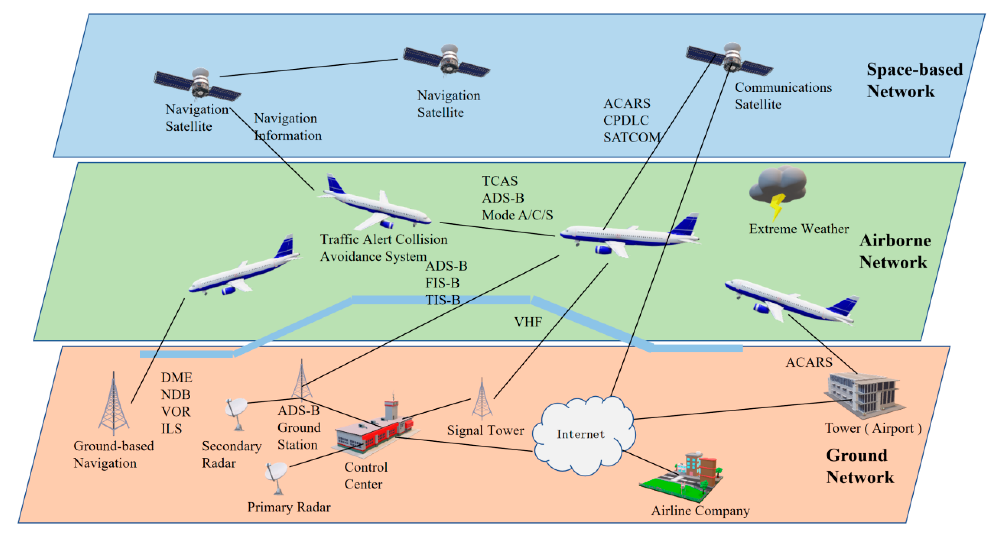
The air traffic management system (ATM) is a typical airspace integration network system [1,2,3] (shown in Figure 1), which plays a significant role in ensuring flight safety and enhancing flight efficiency by monitoring and controlling aircraft flight activities with communication, navigation technologies and monitoring systems. As more and more embedded devices and systems are digitized and connected to many wireless services and communications, attackers are exploiting security vulnerabilities to conduct virus ransom and cyberattacks, posing a serious threat to human travel safety. Meanwhile, air traffic management system cyberattacks are also developing towards a new trend. The degree of automation and attack correlation is constantly improving, and the attack actions are unpredictable. According to the International Threat Report Portugal Q1 2021 [4], malware in the first quarter of 2021 increased by 24.2% compared to the same period last year. According to Check Point’s ransomware report [5], the air transport industry experienced an 186% increase in weekly ransomware attacks between June 2020 and June 2021. A large amount of useful security information such as the international aviation security reports, cyber security vulnerability database, and threat database is seriously fragmented [6], and these resources are not properly integrated and utilized. The current problem of ATM cyber security posture analysis is not the lack of available information, but how to fuse heterogeneous information from multiple sources to achieve ATM cyber security posture analysis and provide auxiliary decision support for penetration testing.
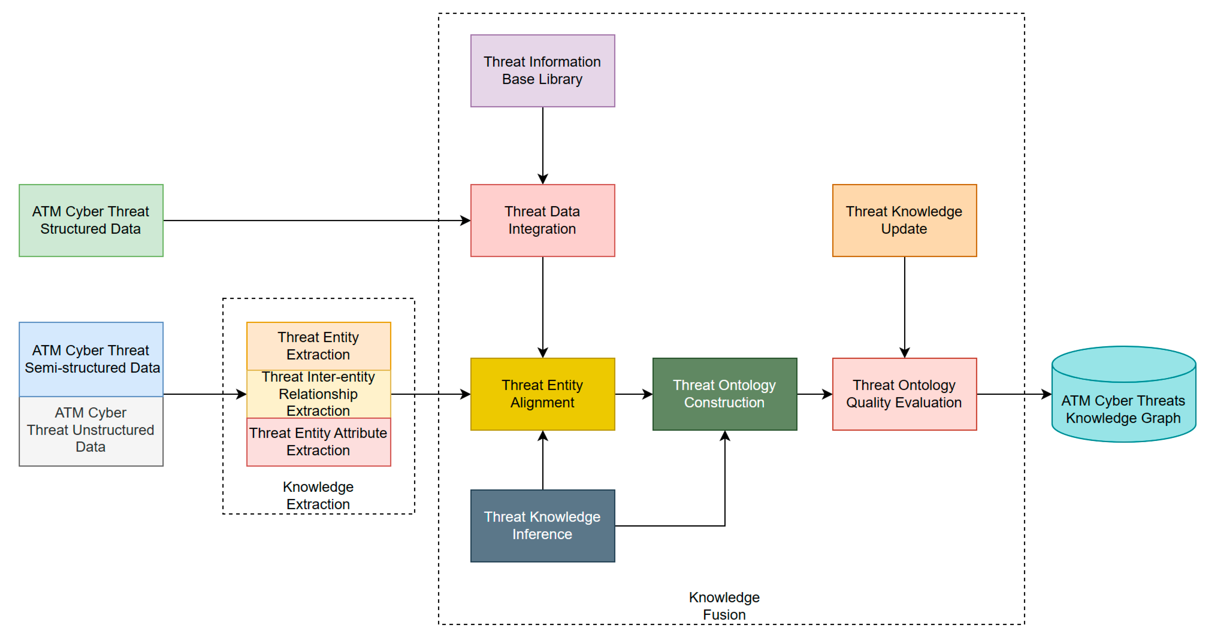
The ATM cyber threat knowledge graph construction includes the processes of knowledge extraction, knowledge fusion, quality assessment, and knowledge graph storage [7] (as shown in Figure 2). Knowledge extraction [8] mainly includes entity recognition, relationship extraction, and attribute extraction. Knowledge fusion techniques include data integration, entity alignment, knowledge modeling, knowledge embedding [9], etc. The construction process includes, firstly, preprocessing unstructured data and semistructured data, conducting knowledge extraction to obtain entities, interentity relationships, entity attributes, and performing integration of structured data with information databases and knowledge databases, and then entity alignment, disambiguation of knowledge, and finally ontology construction and knowledge modeling. Knowledge embedding can be used for entity alignment and ontology construction in the above process. Knowledge modeling is followed by quality assessment, continuously updating knowledge, and ultimately forming a knowledge graph. Through the analysis of the air traffic management system cyber threat knowledge graph, cyber security experts can more intuitively understand the threat intelligence and security posture and discover complex cyberattack patterns.
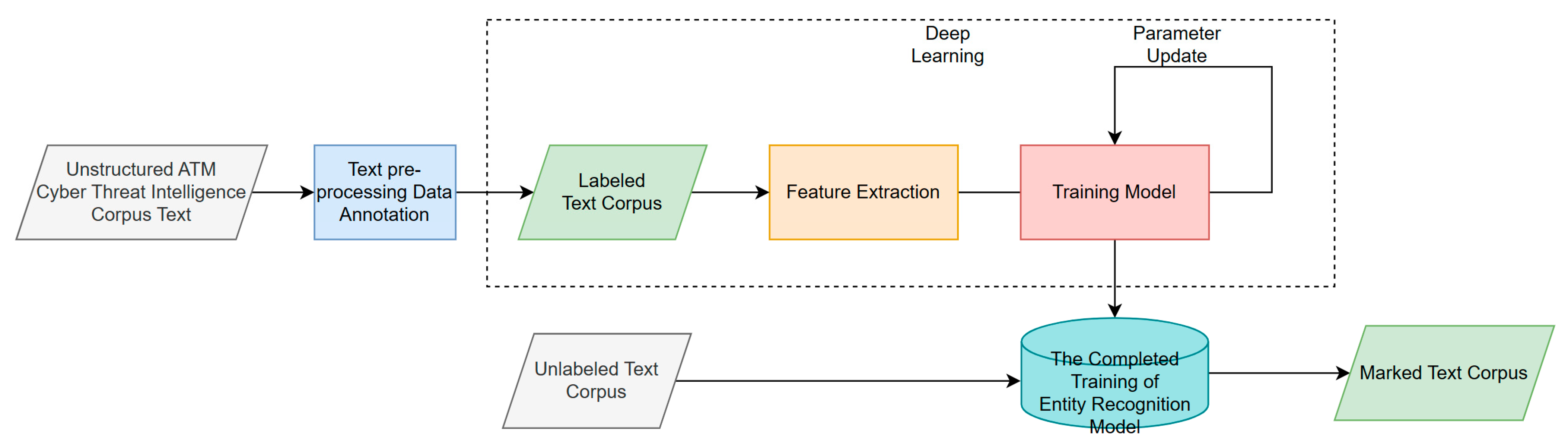
Entity recognition technology is the basis for the construction of the ATM cyber threat knowledge graph. To effectively build the ATM cyber threat knowledge graph, entities must be extracted from massive multisource intelligence data, especially from unstructured data. The principle of ATM cyber threat entity recognition [10] (shown in Figure 3) is as follows: first, preprocess the unstructured ATM cyber threat corpus text, and then, conduct data annotation and labeling. The labeled text corpus is then subjected to deep learning process, and the entity contextual features and entity internal features are extracted by the deep learning method, which is trained iteratively to finally obtain an entity recognition model. The unlabeled text corpus is automatically labeled by the completed training of the entity recognition model; as a result, the category of the entity can be obtained. The entity recognition method by deep learning can fully discover and utilize entity contextual features and entity internal features, and this method is more flexible with better robustness [11]. ATM cyber threat entity recognition is a specific domain entity recognition in the field of named entity recognition. The main task is to recognize different types of threat entities such as malware, URL, IP address, and hash in text data. The purpose is to confirm and classify the professional vocabulary in the field of ATM cyber threats and provide data support for the later construction of knowledge graphs.
The contributions of this paper are summarized into three points:
Firstly, a TextCNN-Flat-Lattice Transformer (TCFLTformer) with CNN-transformer hybrid architecture is proposed for ATM cyber threat recognition entities, in which a relative positional embedding (RPE) is designed to encode position text content information, and a multibranch prediction head (MBPH) is utilized to improve deep feature learning.
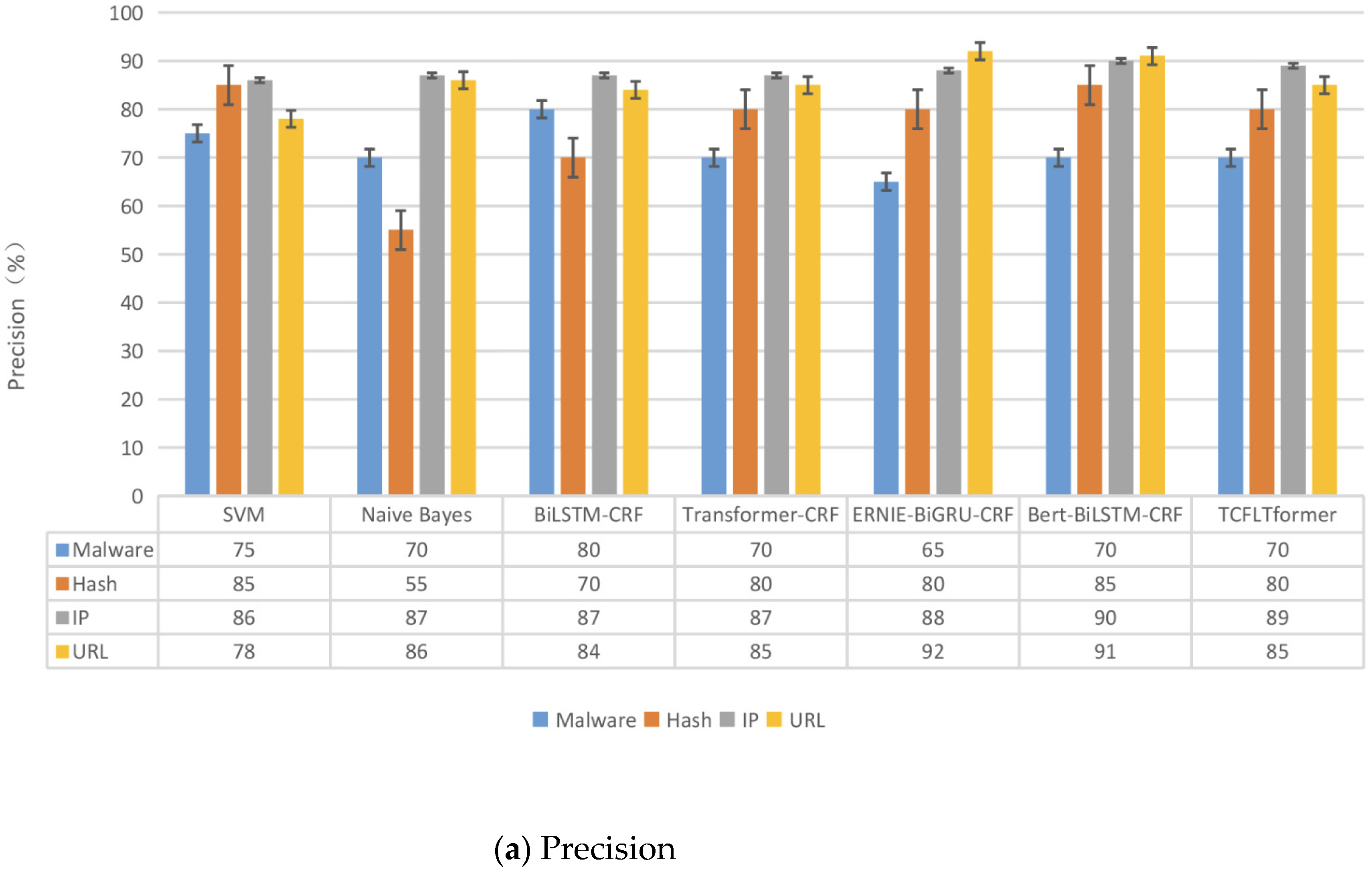
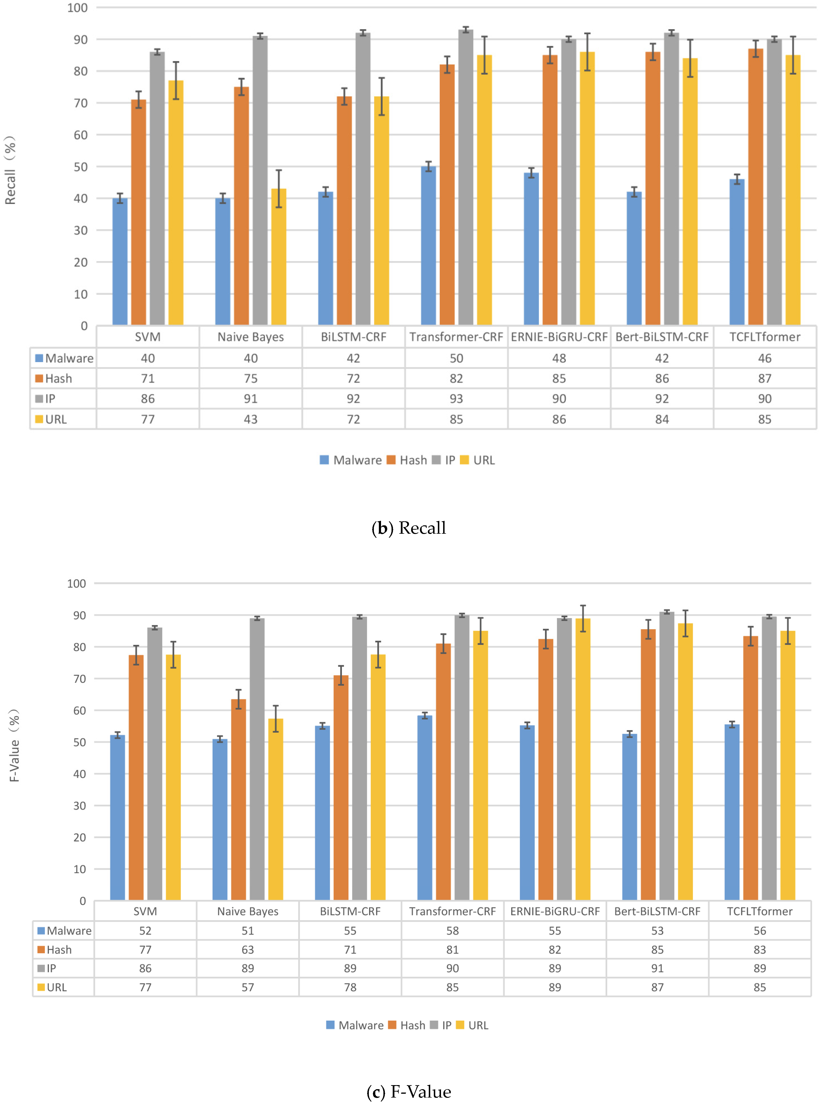
Secondly, ATM cyber threat entity recognition datasets (ATMCTERD) are provided for our research needed, which contain 13,570 sentences, 497,970 words, and 15,720 token entities. We collect data from multiple sources, which are mainly from international aviation authorities and cyber security companies, We manually annotate the datasets with BIO annotation rules, and the annotation entity types are malware, URL, IP address, and hash.
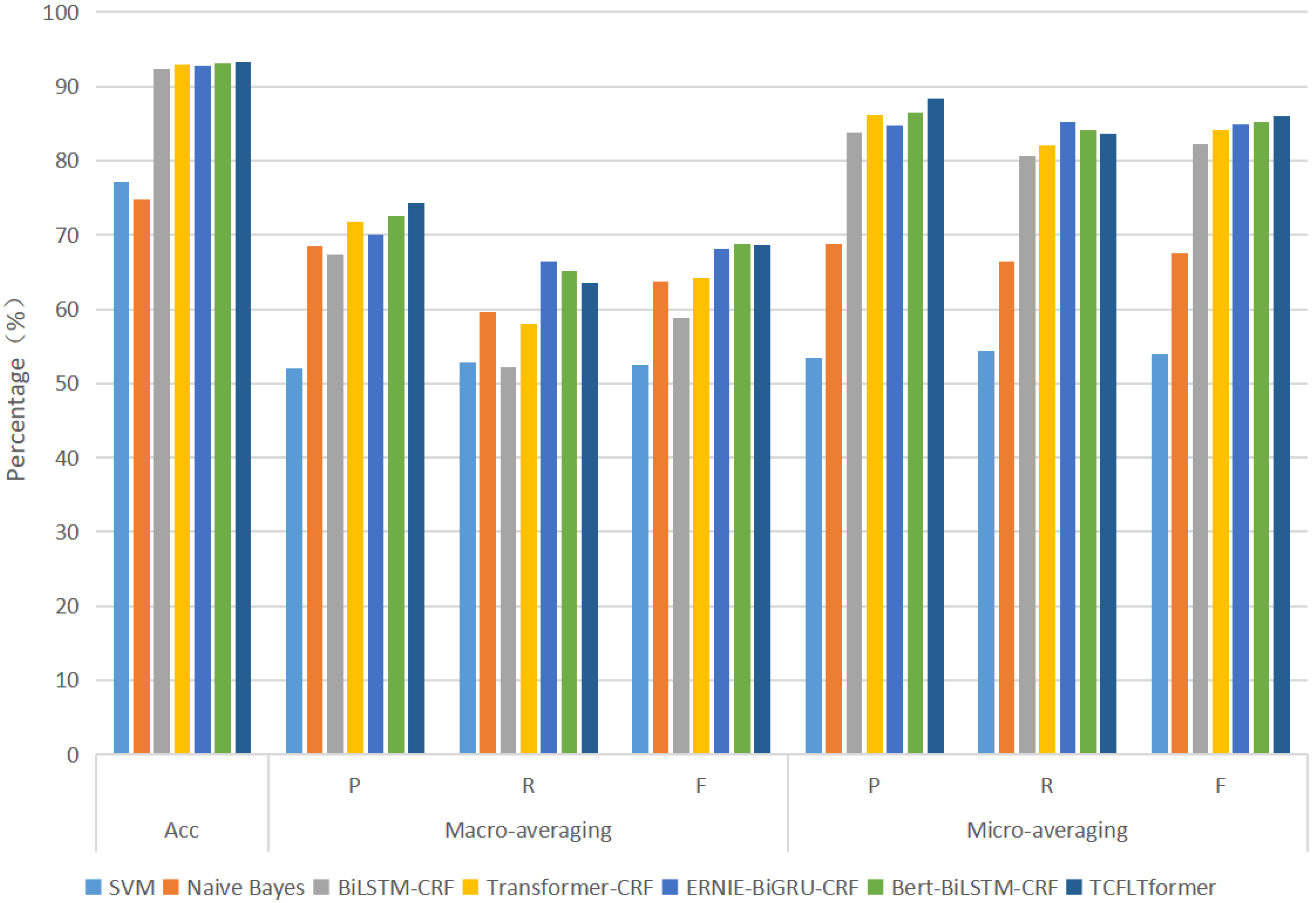
Finally, in comparative experiments with six NER models on our datasets that we proposed, TCFLTformer can obtain the highest accuracy scores of 93.31% and the highest precision scores of 74.29%, while the highest accuracy rate and precision rate of other methods are 93.10% and 72.61%, respectively, which is an improvement of 0.21% in accuracy rate and 1.68% in precision rate. Then, we carry out the additional experiments on MSRA and Boson datasets to fully and comprehensively evaluate the effectiveness of our model. This indicates that the method proposed in this paper can recognize cyber threat entities in the ATM more accurately and better perform.
The rest of the manuscript is organized as follows. Section 2 reveals related work, Section 3 reveals detailed structures of the methodology, while Section 4 gives model training and optimization. The experimental settings and the experimental results are demonstrated and analyzed in Section 5. The discussion part is in Section 6. Finally, we make the conclusions and outlook in Section 7.

2. Related Work

Entity recognition refers to named entity extraction technology, which plays an important role in natural language processing and is the most critical and fundamental process in knowledge extraction. At present, a considerable amount of literature has made some progress and published on entity recognition subject. Based on the development history of entity recognition technology, the main research methods include traditional machine learning methods and deep learning methods.

2.1. Entity Recognition Based on Traditional Machine Learning

Traditional machine learning methods mainly use feature engineering to transform text data into numerical features and then use classifiers for classification. Applying traditional machine learning, entity recognition is cast to a multiclass classification or sequence labeling task. Given labeled data samples, features are carefully designed to represent each training example. Machine learning algorithms are then utilized to learn a model to recognize similar patterns from unstructured data.
Many machine learning algorithms have been applied in entity recognition, including Hidden Markov Models (HMM) [12], Decision Trees [13], Maximum Entropy Models [14], Support Vector Machines (SVM) [15], and Conditional Random Fields (CRF) [16]. McNamee and Mayfield [17] used 1000 language-related and 258 orthography and punctuation features to train SVM classifiers. Each classifier makes a binary decision as to whether the current token belongs to one of the eight classes, i.e., B-(Beginning), I-(Inside) for person, organization, location, and other tags. SVM does not consider “neighboring” words when predicting an entity label. McCallum and Li [18] proposed a feature induction method for CRF in entity recognition. Experiments were performed on CoNLL03 and achieved an F-score of 84.04% for English. The two methods are based on traditional machine learning. However, traditional machine learning methods need to manually select and extract features, and they have limited ability to express text data, so it is difficult to deal with complex semantic information. Hence, there will be error propagation in the model during training. In view of this, scholars gradually began to shift their focus to deep learning.

2.2. Entity Recognition Based on Deep Learning

Deep learning methods have achieved great success in the field of natural language processing, and current mainstream research is based on deep learning approaches to entity recognition, where the nonlinear modeling properties of deep neural networks models facilitate the ability to represent learning and the semantic combination capabilities conferred by vector representation and neural processing, which allows machines to acquire raw data and automatically discover potential representations and processing needed for classification or detection [11]. It can automatically learn intricate hidden feature representations from the input data without complex feature engineering and extensive domain knowledge (i.e., this is done by the partial deep learning model shown in the dashed box in Figure 3), and deep neural networks can automatically capture features for recognition without much human intervention, thus saving a lot of effort.
Researchers have proposed various deep learning algorithms for entity recognition; the application of convolutional neural networks (CNN) to named entity recognition tasks was originally proposed by Collobert in 2019 [19]. In the same year, scholars added CRF based on CNN and proposed the CNN-CRF model, which was used to extract entities from Chinese electronic cases [20]. Both accuracy and speed improved after using this model. In 2021, Kong and Zhang added an attention mechanism to deal with the information loss in long sentences based on the fact that the traditional CNN cannot handle the loss of long-distance information. They proposed a new CNN model, in which the CNN fusion of different convolution kernels and residual structures improved the ability to capture the contextual information of long texts from different dimensions [21]. The features of the text in both past and future directions can be obtained by using the Bidirectional Long Short-Term Memory (BiLSTM) model. Inspired by this, several researchers have carried out considerable research work on this basis. Peng et al. [22] proposed a named entity recognition model combining BiLSTM based on character characteristics with Conditional Random Fields (CRF) in the cyber security domain, using an active learning method, and obtained good results using a small batch of labeled samples. Li [23] proposed a fusion of adversarial active learning for security knowledge triad extraction using the BiLSTM-CRF model for joint entity and relationship extraction, and experiments showed the effectiveness of the scheme.
In recent years, applying the transformer model to entity extraction has also become a hot research topic for scholars in this field. The transformer is mainly implemented by the attention mechanism. The use of transformers for named entity recognition can improve accuracy and shorten the training time. Representatives of using transformers in named entity recognition include the TENER model proposed by Yan [24] and the Transformer-CRF model proposed by Li Bo [25]. The former proposes a special transformer structure for the named entity recognition task, while the latter is used in the transformer. The CRF is introduced for entity classification and recognition based on the extraction of text features. In addition, there is the ERNIE-BiGRU-CRF model proposed by Zhang in 2020 [26] and the BERT-BiLSTM-CRF model proposed by Shen in 2022 [27], both of which combine the attention mechanism with RNN, and the neural networks extract sentence features and uses the attention mechanism to solve the problem of long-distance dependence, effectively improving the capability of overall recognition. The application of the attention mechanism in the named entity recognition task expands the research direction of named entity recognition.

3. Methodology

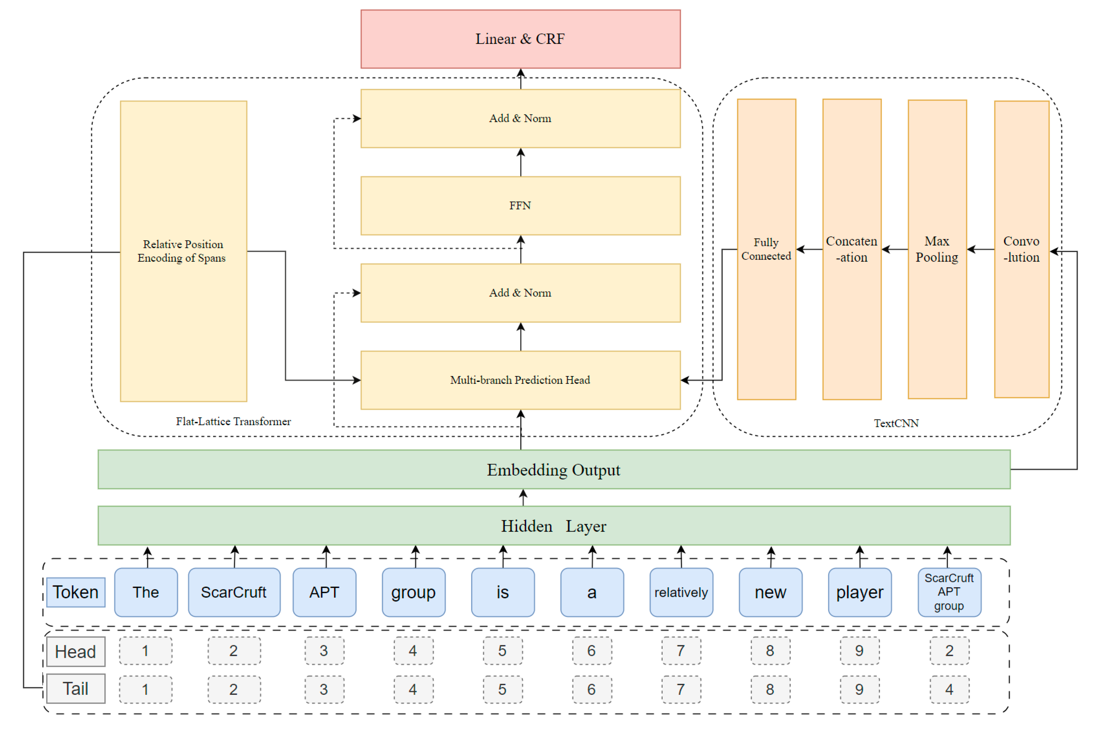
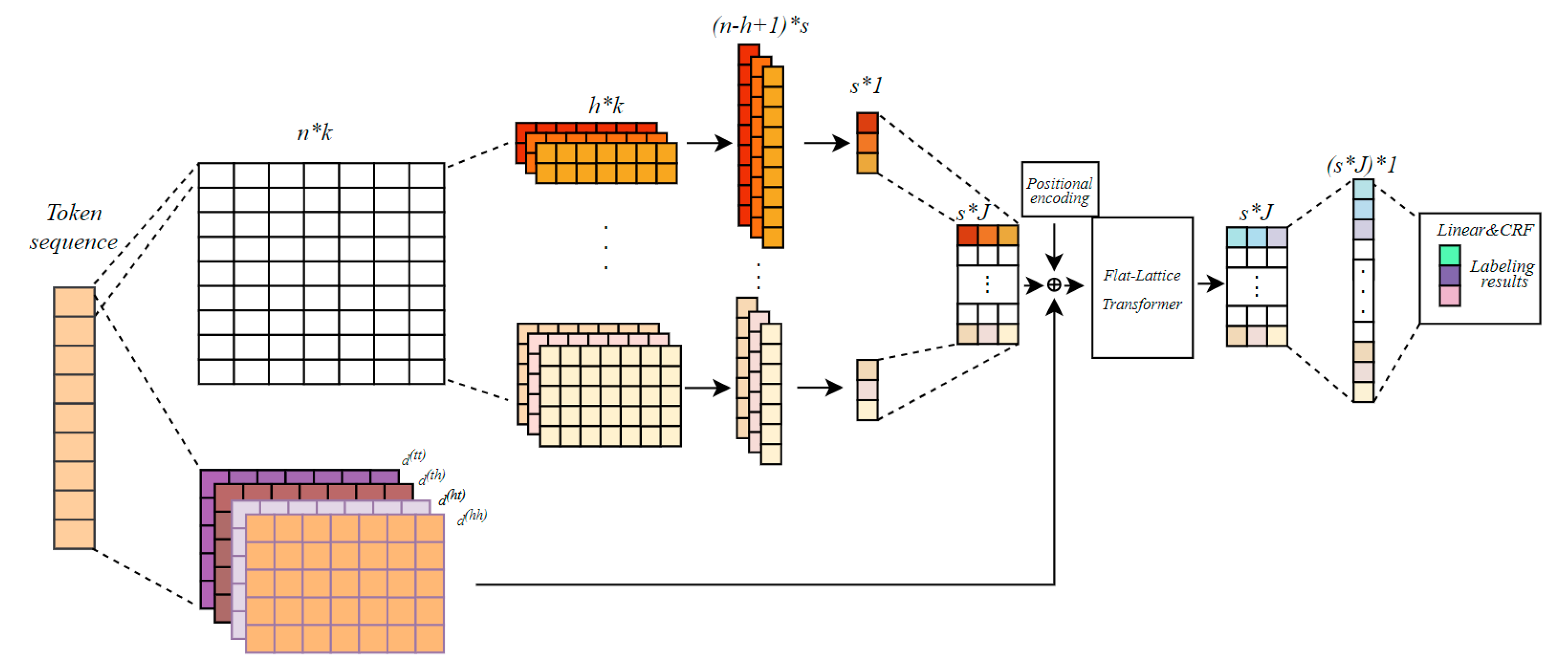
In this paper, we propose a TCFLTformer model for the recognition of ATM cyber threat entities, which can be divided into two parts, the TextCNN module and the Flat-Lattice Transformer module (as shown in Figure 4). Among them, TextCNN [28] is a text model based on a convolutional neural network, which mainly extracts local features from text and enhances the ability of the model to learn to acquire local features. Flat-Lattice Transformer [29] is a flat graph structure model based on Transformer [30], which can process long hierarchical text data. It mainly learns the temporal and relative positional characteristics from the text data. This method combines the advantages of TextCNN and Flat-Lattice Transformer, which can improve the accuracy of recognition cyber threat entities in ATM.
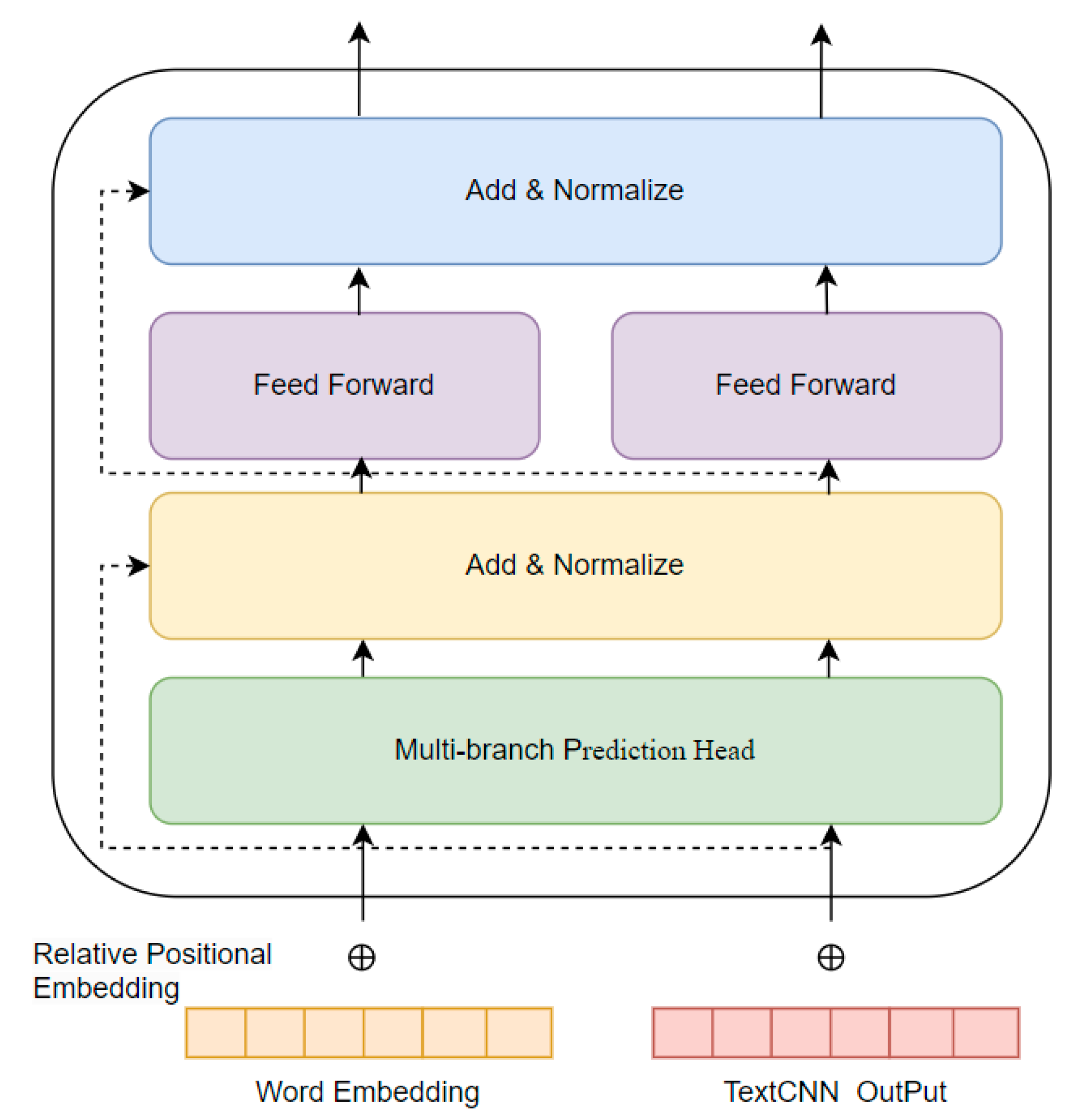
The TCFLTformer model is a deep learning-based entity recognition model, and the principle of this model is shown in Figure 5. Firstly, the text is word-vectorized n × k, and then the TextCNN model is used to extract the cyber threat entity features in the ATM. In the process of feature extraction, we use multiple convolution kernels of different sizes h × k for convolution operation to capture the text features of different lengths (nh + 1) × s of text features, and the features s × 1 obtained from the convolution operation are pooled, the convolution operation can extract local features, and the pooling operation can downscale the features to reduce the number of parameters of the model. Then, the feature vectors are input into the fully connected layer to obtain fixed-length feature vectors s × J, then they are input into the multibranch prediction head, then they are processed by the Flat-Lattice Transformer model processing, and finally, the labeling results of the input entities are obtained after probabilistic judgment of the linear CRF layer.
It is noteworthy that the input of the multibranch prediction head (MBPH) of the TCFLTformer module has two parts, as shown in Figure 6: one is the word vector matrix and the relative position encoding matrix composed of the ATM cyber threat entities, the other is the output matrix of the fully connected TextCNN module, which fully learns the entity features through the two parts of matrix data to obtain a richer feature representation and enhance the model. The details of each network layer of the model are as follows:
① Token Embedding
We use character-level N-gram [31] to represent a word. For example, the word “scarcruft”, assuming the value of n is 3, has the trigram “<sc”, “sca”, “car”, “arc”, “rcr”, “cru”, “ruf”, “uft”, and “ft>”, where “<” is the prefix and “>” is the suffix. Thus, we use these trigrams to represent the word “scarcruft”, and here the vector of 9 trigrams can be superimposed to represent the word vector of “scarcruft”. The word vectorization hierarchy is the same as the CBOW [32] structure and consists of three layers: an input layer, an implicit layer, and an output layer, where the input layer is multiple words represented by vectors and their N-gram features and location features, the implicit layer has only one layer (shown in Figure 4), which is a superimposed average of multiple word vectors, and the output layer is the word vector corresponding to the completion of processing.
The e i R k is the k-dimensional word vector corresponding to the i-th word in a sentence. A sequence of length n can be expressed as a matrix E 1 : n = ( e 1 T , e 2 T , , e n T ) T R n k . Then, the matrix E 1 : n is taken as the input into the convolution layer.
② TextCNN
In the convolution layer, J filters of different sizes are convolved E 1 : n to extract local features. The width of each filter window is the same E 1 : n , only the height is different. In this way, different filters can obtain relationships for different ranges of words. Each filter has S ( s S ) , a convolution kernel. Convolutional neural networks learn parameters in a convolutional kernel, with each filter having its focus, allowing multiple filters to learn multiple different pieces of information. We designed multiple convolutional kernels of the same size to learn features complementary to each other from the same window. The specific formula is as follows:
C i j = f ( W j E i : i + h 1 + b )
where W j R h k denotes the weight of the j-th ( j J ) filter of the convolution operation, C i j is the new feature resulting from the convolution operation, b R is a bias, and f is a nonlinear function. Many filters with varying window sizes slide over the full rows E 1 : n , generating a feature map C 1 j , C 2 j , , C n h + 1 j . The most important feature C s j was obtained by one-max pooling for one scalar and mathematically written as:
C s j = M a x ( [ C 1 j , C 2 j , , C n h + 1 j ] )
S convolution kernels are computed to obtain S feature values, which are concatenated to obtain a feature vector Pj:
P j = [ C 1 j , C 2 j , , C S j ]
Finally, the feature vector of all filters is stacked into a complete feature mapping matrix M R J S :
M = [ P 1 , P 2 , , P j ]
③ multibranch prediction Head (MBPH)
For ease of exposition, according to Figure 6, the input consists of a word vector matrix referred to as F R b c h w , the TextCNN layer output feature mapping matrix referred to as F R b l h w . Then, both F and F′ will be reshaped, referred to as f R b c ( h w ) and f R b l ( h w ) . Finally, f and f will be turned into a token embedding through einsum operation, which can be denoted as:
t b l c = f b l ( h w ) f b c ( h w )
where l is the token length, and b, c, h, and w denote the batch size, number of channels, height, and width of the input feature F.
The MBPH first expands t into a new embedding t′ by a linear layer, which can be denoted as:
t = t W l , t R b l ( n d 3 )
where W l is the weight of the linear layer, n is the head number of MBPH, and d is the dimension for subsequent tensors.
Then, the embedding t′ will be forwarded to different heads. Parameters are not shared among heads. Each head contains two steps: linear transformation and scale dot-product attention (SDPA).
The linear layers are applied to map t′ into a query ( Q R b n l d ), key ( K R b n l d ), and value ( V R b n l d ), which can be denoted as:
Q , K , V = t W Q , t W K , t W V
where W Q , W K , W V denotes the weights of the linear layers to map Q, K, and V, respectively.
Thereafter, the correlation between them is calculated through dot-product operation and softmax activation to generate an attention map, which will be used as the weight V. The process can be expressed as:
S D P A ( Q , K , V ) = S o f t m a x Q k T d V
The output of each head will be concatenated together before a linear layer is applied, then we will obtain the final output of the MBPH, which can be expressed by the following formula:
h e a d m = S D P A ( t W m Q , t W m K , t W m V ) , m ( 0 , n ]
M B P H ( Q , K , V ) = C o n c a t ( h e a d 1 , , h e a d n ) W o
where W Q , W K , W V denotes the weights of the linear layers of the m-th head to map Q, K, and V, respectively. W o is the weight of the last linear layer in MBPH.
④ Relative Position Embedding
While the original Transformer captures sequence information by absolute position encoding, we use Lattice’s relative position for encoding [33]. The flat-lattice structure consists of spans of different lengths. To encode the interactions between spans, the relative position of the spans is encoded. For two spans xi and xj in the lattice, there are three relationships between them—intersection, inclusion, and separation—and dense vectors are used to model the relationship between them. For example, head[i] and tail[i] denote the head and tail positions of span xi, and then the relationship between the two spans xi and xj is expressed in terms of four relative distances, which are calculated as:
d i j ( h h ) = h e a d [ i ] h e a d [ j ]
d i j ( h t ) = h e a d [ i ] t a i l [ j ]
d i j ( t h ) = t a i l [ i ] h e a d [ j ]
d i j ( t t ) = t a i l [ i ] t a i l [ j ]
d i j ( h h ) denotes the distance between the head of xi and the head of xj, d i j ( h t ) denotes the distance between the head of xi and the tail of xj, and the same for others. The final relative position encoding is a simple nonlinear transformation of the four distances, which are calculated as:
R i j = R e L U ( W r ( P d i j ( h h ) P d i j ( h t ) P d i j ( t h ) P d i j ( t t ) ) )
where W r is the learnable parameter, ⊕ is the connection operator, Pd is computed by referring to [30], and then the positions of the words composing the sequence are encoded to obtain the corresponding positional embedding [29], which is computed as the following equation:
P E ( p o s , 2 i ) = sin p o s 10000 2 i / d e m b
P E ( p o s , 2 i + 1 ) = cos p o s 10000 2 i / d e m b
where pos denotes the sequential position of the word, and i is the dimensional index of the positional encoding, denoting the i-th dimension of the word vector, i ∈ [0, d e m b −1], where the dimension of the positional embedding coincides with the dimension of the word vector. It is then summed with the word vector of the corresponding input so that the distance between words can be characterized for the model to learn to understand the order of information between the input words.
A i , j = W q T E x i T E x j W k , E + W q T E x i T R i j W k , R + u T E x j W k , E + v T R i j W k , R
where W q , W k , R , W k , E R d e m b d h e a d is the learnable parameter, and then A is replaced by A*.
A t t ( A , V ) = s o f t m a x ( A ) V
⑤ Residual Connection
A residual connection has also been added to the model, as shown in Figure 6, for the add operation. Suppose the output of a layer in the encoder is f(x) for a nonlinear variation of the input x. Then, after adding the residual connection, the output becomes f(x) + x. The +x operation is equivalent to a shortcut. The purpose of adding the residual structure is mainly to avoid the gradient vanishing problem when updating the model parameters during backpropagation: thanks to the residual connection, an additional term x is added to the output, then the layer network can generate a constant term when biasing the input, and thus will not cause gradient vanishing when applying the chain rule during backpropagation.
⑥ Layer Normalization
In deep learning, there are various ways to handle data normalization, but they all have a common purpose: they want the input data to fall in the nonsaturated region of the nonlinear activation function, and therefore transform it into data that obey a distribution with a mean of 0 and a variance of 1.
Layer normalization is processed for a single sample, and the number of hidden layer nodes in a layer is denoted by H. ai denotes the output of the i-th hidden layer node, and the statistics in layer normalization can be calculated using the following formula:
μ = 1 H i = 1 H a i
σ = 1 H i = 1 H ( a i μ ) 2
Using Equation (21) to calculate the layer-normalized values through μ and σ:
a i ¯ = a i u σ 2 + ε
where ε is a very small number to avoid the denominator being 0. It is worth pointing out that the calculation of layer normalization is not related to the number of samples, it only depends on the number of hidden layer nodes, so as long as the number of hidden layer nodes is guaranteed to be sufficient, the statistics of layer normalization can be guaranteed to be representative enough.
⑦ Feed-Forward Neural Network Module
This paper refers to the design of the Transformer encoder. It implements the feed-forward neural network (FFN) submodule of the inattention encoder, using two fully connected layers. The first layer uses ReLU as the activation function, and the second layer uses a linear activation function. If the input of the feed-forward neural network is denoted by Z, the output of the feed-forward neural network can be expressed as follows:
F F N ( Z ) = R e L U ( Z W 1 + b 1 ) W 2 + b 2
where W1 and W2 are the weight matrices of each layer, and b1 and b2 are their corresponding biases.
In addition, we also use residual connection and layer normalization in the above two submodules to speed up the convergence of network training and prevent the gradient vanishing problem:
O u t P u t = L a y e r N o r m ( X + S u b M o d u l e ( X ) )
where X are the outputs of the above two submodules.
⑧ Linear CRF
The basic form of the linear chain conditional random field model parameters P y x is defined as follows:
P y x = 1 Z ( x ) e x p i , k λ k t k y i 1 , y i , x , i + i , ι u ι s ι y i , x , i
Z x = y Y e x p i , k λ k t k y i 1 , y i , x , i + i , ι u ι s ι y i , x , i
where t k y i 1 , y i , x , i denotes the transfer feature function defined on the edge, which is related to the current position and the previous position i 1. The state feature function defined on the node represented by s ι y i , x , i is only relevant to the current position i . In general, the characteristic function takes the value of 1 when the corresponding conditions are met, otherwise, it is 0. λ k and u ι are the feature functions and the corresponding weights, respectively, whose values are updated during the training process [34]. Equation (26) is the normalized factor term whose value corresponds to the summation of scores using the characteristic function for all possible candidate state sequences.
For the sequence annotation task, given a linear chain of conditional random fields λ , an input text sequence x, and a set y of all possible candidate annotation results, the desired optimal annotation result y , as in Equation (28), can be computed quickly and efficiently using the Viterbi algorithm.
y = argmaxP y Y y x , λ
y = argmax y Y i , k λ k t k y i 1 , y i , x , i + i , ι u ι s ι y i , x , i

4. Model Training and Optimization

To train and optimize our proposed TCFLTformer cyber threat entity recognition model for ATM, we used the following steps:

4.1. Data Preprocessing

Before model training, we need to preprocess the data of the air traffic management system cyber threat entity recognition task. To ensure the diversity and breadth of the datasets, we have collected data from multiple sources shown in Table 1, which are mainly from international aviation authorities and cyber security companies, such as the National Aeronautics and Space Administration (NASA), Single European Sky ATM Research (SESAR), Federal Aviation Administration (FAA), European Aviation Safety Agency (EASA), Microsoft Security, Naked Security, Quick Heal Antivirus Blog, etc., who have published unstructured cyber threat intelligence (CTI) reports and articles that contain a large number of ATM system cyber threat entities. The number of aviation authority and security company blogs and their articles collected are shown in Table A1 (Appendix A) with websites in this paper. The texts in the datasets are all in English, which contain a large number of technical terms and acronyms. We have manually annotated the datasets with the BIO-tagging, where each token is labeled as B (beginning), I (inside), or O (outside) of an entity, and the four types of annotation entity are malware, URL, IP address, and hash. To ensure the quality and reliability of the datasets, the annotation results have been reviewed and verified several times.

4.2. Training Process

We used the PyTorch deep learning framework to implement the model training, using the Adam optimizer to optimize the parameters of the model and setting the learning rate to 0.001. We also used a cross-entropy loss function to calculate the loss values of the model. We used a batch gradient descent algorithm to update the parameters of the model during training, with each batch of size 64. We used a GPU to accelerate the training process of the model for faster convergence. We trained 50 epochs, each epoch containing multiple batches. At the end of each epoch, we recorded the loss value and accuracy of the model for model tuning and validation. Table 2 shows the model algorithm training process.

4.3. Model Optimization

To further improve the performance of the model, the following optimization strategies were used:

4.3.1. Dropout

We added a Dropout layer between the fully connected and convolutional layers of the model to avoid overfitting, and we set the probability of Dropout to 0.5.

4.3.2. Learning Rate Adjustment

A learning rate adjustment strategy was used during the training process to better control the training speed of the model. We used the StepLR scheduler to adjust the learning rate by dividing the learning rate by 10 at the end of each epoch.

4.3.3. Regularization

L2 regularization was used to control the complexity of the model to avoid overfitting, and the regularization factor was set to 0.001.

4.3.4. Model Evaluation

According to the annotation model of BIO, malware, URL, IP address, and hash are divided into four separate issues, and each problem is divided into a triple classification problem. Take malware as an example: it is divided into three categories such as B-Malware, I-Malware, and O. The initial word B-Malware and the noninitial word I-Malware of the recognized malware are combined into one entity, and the complete recognition of a security entity is correctly recognized. In addition, only recognized entities with the initial word B-Malware, and noninitial words I-Malware and O, are not considered to be correctly recognized. Therefore, the evaluation index system commonly used in multiclassification problems will be used to evaluate the recognition effect of the cyber security entity recognition model studied in this paper.
After the model is trained, we use a test set to evaluate the model. We calculated the accuracy, recall, F-value, macroaverage, and microaverage metrics of the model to evaluate the performance of the model. The Accuracy (ACC) is the ratio of the number of samples correctly classified by the classifier to the total number of samples, the Precision (P) is the ratio of the number of positive samples correctly classified by the classifier to the number of positive samples predicted by the classifier, the Recall (R) is the ratio of the number of positive samples correctly classified by the classifier to the number of true positive samples, and the F-value is the summed average of Precision and Recall, and is one of the most commonly used metrics to evaluate model performance.
The main evaluation metrics [29] used in this paper are Precision (P), Recall (R), F-value (F), Accuracy (Acc), Macroaveraging, and Microaveraging. The specific calculations are shown below:
P = T P / ( T P + F P )
R = T P / ( T P + F N )
F = ( 2 × P × R ) / ( P + R )
A c c = ( T P + T N ) / ( T P + T N + F P + F N )
Macroaveraging, which first calculates the value of each class statistical indicator and then finds the arithmetic mean for all classes, is calculated as follows:
M a c r o P = 1 n i = 1 n p i
M a c r o R = 1 n i = 1 n R i
M a c r o F = 1 n i = 1 n F i
where n is the number of entity types, and there are four types of entities in this paper, so n is 4. Pi, Ri, and Fi denote the Precision, Recall, and F-value for the i-th type of entity.
Microaveraging unclassified statistics for each of the test data, and then calculating the corresponding index, the calculation formula is as follows:
M i c r o P = i = 1 n T P i i = 1 n T P i + i = 1 n F P i
M i c r o R = i = 1 n T P i i = 1 n T P i + i = 1 n F N i
M i c r o F = 2 × M i c r o P × M i c r o R M i c r o P + M i c r o R

5. Experiment

5.1. Experimental Environment

The experimental environment for this article is a computer with an Intel(R) Core(TM) i7-8700K CPU @ 3.70 GHz processor, 32 GB of RAM, and NVIDIA GeForce GTX 1080 Ti graphics card. The operating system is Ubuntu 18.04 LTS.

5.2. Experimental Data

In our experiments, we divide the dataset with completed data preprocessing into the training set, validation set, and test set in the ratio of 7:1:2, where the training set is used to train the model, the validation set is used to estimate the training level of the model and optimize the parameters, and the test set is used to evaluate the performance of the model. The training set consists of 9499 sentences, 348,579 words, and 11,004 token entities, the validation set consists of 1357 sentences, 49,803 words, and 1373 token entities, and the test set consists of 2714 sentences, 99,588 words, and 3343 token entities, as shown in Table 3.
We perform categorical data analysis on the datasets, which are formatted into two columns, with words and corresponding labels for each row. The sentences are separated by spaces and line breaks. The number and percentage of each type of tagged entity are shown in Table 4. The number of malware entities is 6991, or 44.47%; the number of hash entities is 3378, or 21.49%; the number of URL entities is 4363, or 27.75%; and the number of IP entities is 988, or 6.28%.

5.3. Experimental Setup

The experiments use a TCFLTformer cyber threat entity recognition method for ATM in this paper. We have used a cross-validation method to ensure the generalization capability and reliability of the model.
In training the model, we used the Adam optimizer with a learning rate of 0.001 and a batch size of 64. To prevent overfitting, we used an early-stop strategy and the Dropout technique. Specifically, training was stopped when the model performance on the validation set did not improve for 10 consecutive epochs.

5.4. Experimental Method

To verify the recognition effectiveness of the TCFLTformer cyber threat entity recognition model for ATM proposed in this paper, comparison experiments are conducted on different algorithmic models. The comparison models in the experiments include SVM [35], Naive Bayes [36], BiLSTM-CRF [37], Transformer-CRF [25], ERNIE-BiGRU-CRF [38], BERT-BiLSTM-CRF [39], and the proposed paper based on the TCFLTformer deep learning models; all comparison models are trained and tested on the same datasets. To exclude the randomness of the model training process, and exclude whether the tiny edge (if there is one) is due to the chance or randomness of the experiment, we take the average of the results of the 20 experiments as the final result, and the results of the accuracy evaluation related to the 20 experiments are shown in Table 5.

5.5. Model Evaluation Results

Firstly, we compare the approach proposed in this paper with the traditional feature engineering machine learning model. Table 6 shows the experimental results of the test set on different models (best in bold), and Figure 7 shows the comparison of the experimental results on different models. From the experimental results, the accuracy of the method proposed in this paper reaches 93.31%, the recall R reaches 63.63%, and the F-value reaches 68.55%, while the accuracy of the traditional method SVM is only 77.20%, the recall R is 52.90%, and the F-value is 52.50%. It can be seen that the traditional machine learning model performs poorly in the threat entity recognition task, with a lower accuracy, precision, recall, and F-value than the deep learning model. The reason for this result is that the traditional machine learning methods mainly use feature engineering to transform text data into numerical features and then use classifiers to classify them, and the method has limited expressiveness for text data and has difficulty in handling complex semantic information. In conclusion, it indicates that the method proposed in this paper can recognize cyber threat entities in the ATM more accurately and better perform than the traditional feature engineering machine learning model.
Secondly, we compare the method proposed in this paper with other deep learning methods. The experimental results show that the method in this paper has certain advantages in terms of accuracy and precision rate. Specifically, the accuracy rate of the method in this paper is 93.31%, and the precision rate is 74.29%, while the highest accuracy rate and precision rate of other methods are 93.10% and 72.61%, respectively, which is an improvement of 0.21% in accuracy rate and 1.68% in precision rate. Next, we give some detailed analysis of the performance with different algorithmic networks which were trained and tested on the same datasets.
  • BiLSTM-CRF [37]: The model is a sequence labeling model based on LSTM networks, which combines BiLSTM networks and CRF (Conditional Random Fields) for labeling input sequences. The BiLSTM network can capture the input sequence context information and model the input, while the CRF model can utilize the interdependencies among the labels in the sequence labeling task to globally label the output. From the experimental results, the accuracy of the TCFLTformer reaches 93.31%, the precision P reaches 74.29%, the recall R reaches 63.63%, and the F-value reaches 68.55%, while the accuracy of the BiLSTM-CRF is 92.36%, the precision P reaches 67.38%, the recall R is 52.21%, and the F-value is 58.83%. The reason for such a result is that BiLSTM-CRF may have label sequences annotation ambiguity problems, which are not easy to handle for longer input sequences and may lead to unstable model training and performance degradation.
  • Transformer-CRF [25]: The model is a sequence annotation model based on the Transformer model. It uses the same structure as commonly used in natural language processing for the task of sequence annotation by adding a CRF model to the Transformer model. The transformer is used for modeling, which captures global contextual information. The CRF layer captures the relationships between tags. The results in Table 5 show that the accuracy of the TCFLTformer reaches 93.31%, the precision P reaches 74.29%, the recall R reaches 63.63%, and the F-value reaches 68.55%, while the accuracy of the Transformer-CRF is 92.95%, the precision P reaches 71.78%, the recall R is 58.04%, and the F-value is 64.18%. The reason for such experimental results may be due to the lack of relative position modeling features of the model, resulting in possible difficulties in capturing position relationships and long-term dependencies in some contextual sequences.
  • ERNIE-BiGRU-CRF [38]: The model is a sequence annotation model based on the pretraining model ERNIE and BiGRU network. It combines the pretraining model, bidirectional GRU model, and CRF model. The pretraining model can effectively extract the semantic information in the input sequence, while BiGRU is used for modeling. From the experimental results, the accuracy of the TCFLTformer reaches 93.31%, the precision P reaches 74.29%, the recall R reaches 63.63%, and the F-value reaches 68.55%, while the accuracy of the ERNIE-BiGRU-CRF is 92.83%, the precision P reaches 69.98%, the recall R is 66.39%, and the F-value is 68.14%, respectively, the recall R which is higher by 2.76%. The reason for this experimental result is that the model incorporates the ERNIE pretraining model, which is able to introduce more linguistic information into the entity recognition task and effectively extract the semantic information in the input sequence, and BiGRU for modeling, which is able to capture more complex contextual dependencies; however, the lack of text relative position information extraction is a problem.
  • BERT-BiLSTM-CRF [39]: The model is a sequence annotation model based on the pretrained model BERT, BiLSTM network, and CRF model. It introduces the knowledge of the pretrained model, is able to extract richer semantic information through self-supervised training and joint learning of multiple tasks, and uses BiLSTM modeling with the advantage of bidirectional modeling. The CRF model is also used for the global optimization of annotation results. The results in Table 5 show that the accuracy of the TCFLTformer reaches 93.31%, the precision P reaches 74.29%, the recall R reaches 63.63%, and the F-value reaches 68.55%, while the accuracy of the BERT-BiLSTM-CRF is 93.10%, the precision P reaches 72.61%, the recall R is 65.23%, and the F-value is 68.72%, respectively, the F-value which is higher by 0.17%. The reason for this experimental result is that the model introduces the BERT pretraining model as an encoder, which is able to extract richer semantic information through self-supervised training and joint learning of multiple tasks, and uses BiLSTM modeling, which has the advantage of bidirectional modeling, but may not be effective in recognizing some low-frequency words and, in addition, lacks the feature of relative position modeling, which may be difficult to capture the position relations and long-term dependencies in some contextual sequences.
Then, we compare the experimental results of the four types of ATM cyber threat entities on different models, and Figure 8 shows the experimental results of the four types of threat entities on different models. Among them, the IP entity has the highest F-value, which indicates the effectiveness of the character features extracted by TextCNN. The character-level vectors extracted by the model can represent the morphological features to a certain extent, so that the relevant features can be fully obtained for such threat entities with mixed numeric–symbolic, fixed-format characteristics, thus improving the F-value of entity recognition.
Finally, we conducted an error analysis of the experimental results. The experimental results show that there are two main errors in the recognition of entities in the ATM by the method in this paper: one is the recognition of nonthreat entities as threat entities, and the other is the recognition of threat entities as nonthreat entities. Among them, the error of recognizing nonthreat entities as threat entities is mainly due to the existence of some entities similar to threat entities in the ATM, while the error of recognizing threat entities as nonthreat entities is mainly due to the lack of obvious features of threat entities or the lack of rich contextual information. To address these errors, we can further improve the recognition effect later by increasing the feature dimension, optimizing the model structure, and increasing the datasets volume.
In summary, the TCFLTformer cyber threat entity recognition method for ATM proposed in this paper has achieved better results in the experiments and has a certain application value.

5.6. Additional Experiments

In order to fully and comprehensively evaluate the effectiveness of the model, we conduct additional experiments with datasets of different sizes, different corpus sources, and different coverage of division granularity. In this paper, we introduce MSRA and Boson public named entity recognition datasets and classify MSRA as a large dataset and Boson as a small dataset according to the corpus size. Among them, Boson is sliced according to the ratio of 8:1:1 for training, validation, and testing sets. Table 7 shows the detailed statistics of each dataset in the experiment.
In the experiment, the MSRA corpus is more standardized, and too large a learning rate can easily lead to the model failing to converge, so the experimental hyperparameters are set as follows: the learning rate of the MASA in the experiment is set to 0.0005, the learning rate of the Boson is set to 0.0015. The maximum length of the training input text is 128; a dropout layer with a rate of 0.1 is added to prevent overfitting; the Bi-LSTM hidden layer dimension is 200; the batch size is set to 24, epoch is set to 60; using the Adam optimizer to update the neural network parameters to minimize the loss function. In order to exclude the randomness of the model training process, we take the average of the results of 20 experiments as the final result shown in Table 8.
It can be seen that the method in this paper is better than other models including the overall performance. Specifically, on Boson, the precision rate of the method in this paper is 89.993%, the recall rate is 92.094% and the F-value is 91.031%, while the highest precision rate of other methods is 88.653%, the recall rate and the F-value of other methods are 91.701% and 90.143%, respectively, which is an improvement of 1.34% in precision rate, 0.40% in recall rate, and 0.89% in F-value rate. Frankly speaking, models such as ERNIE-BiGRU-CRF and BERT-BiLSTM-CRF are already the state-of-the-art methods in the literature at present, so a negligible performance improvement of our model is already good progress.
We compare and analyze the models of our experiments in different aspects. In addition to the improvement of performance indicators, there are also advantages in the aspects below:
(1)
In terms of model size, ERNIE-BiGRU-CRF and BERT-BiLSTM-CRF are both large models based on pretraining, they use a large number of parameters in the training process, which take up more storage space, and TCFLTformer is a small model with better applicability.
(2)
In terms of model construction, ERNIE is trained on a large-scale general-purpose corpus, which may not perform well for some domain-specific tasks. Mask in BERT replaces individual characters instead of entities or phrases, and does not consider lexical structure/grammatical structure. TCFLTformer utilizes the Lattice structure to model the input text, which can better capture the semantic and structural information.
(3)
In terms of model training time, pretrained models require a large amount of computational resources and take a long time to complete the training process; TCFLTformer can compute different parts of the input text in parallel, which accelerates the process of model training and reasoning, and allows more data to be processed in less time.
In summary, the TCFLTformer cyber threat entity recognition method for ATM proposed in this paper has better performance and practicality and provides an effective solution for entity recognition.

5.7. Instances of ATM Cyber Threat Entity Extraction

The threat entities in the text data are extracted by training the cyber threat entity recognition model of the ATM, and Figure 9 shows the word clouds map formed by the four types of threat entities extracted in this paper.
From Figure 9, we can see that malware entities account for the largest proportion of the four types of ATM cyber threats, such as DustySky, VirusTotal, ClearSky, ScarCruft, and other malware. The second proportion is the threat entity hash address, such as db1156b072d58acdac1aeab9af2160a2, 5689448b4b6260ec9c35f129df8b8f2622c66a45, and 331eca9c7d9fd9cbe7cd192af09880a3. The number of threat entities which include the URL and IP categories is shown to be relatively low.

6. Discussion

In this part, we will discuss two widely concerned issues around the safety of air traffic management system (ATM).
  • The risks to civil aircraft from military interventions
Military interventions may occur in any State at any time and pose risks to civil aviation. For example, downing Ukrainian Flight 752 took place in Iranian airspace on 8 January 2020; moreover, downing Malaysia Airlines Flight 17 (MH-17) happened in Ukraine, on 17 July 2014. We briefly discuss the impact of military intervention in conflict zones relating to aviation safety.
1.1 The risk of surface-to-air missiles
The principal weapons of concern for these purposes are those surface-to-air missiles (SAMs) with the capability of reaching aircraft at cruising altitudes (which for these purposes are taken to be altitudes in excess of 25,000 ft (7600 m) above ground level). These are large, expensive, and complex pieces of military equipment which are designed to be operated by trained personnel. In this context, civil aircraft represent a relatively easy and highly vulnerable target, due to their size and predictable flight paths.
1.2 The risk of intentional attack
Some terrorist groups are known to have a continuing and active interest in attacking civil aviation. Such terrorist groups tend to conflict where there is a breakdown of State control. Should they at some point succeed along with the capability to operate them, the vulnerability of aircraft using airspace over those areas to identify and target specific aircraft or aircraft would be high operators with some reliability and would be relatively straightforward. The risk to civil aircraft in those circumstances could immediately become high.
1.3 The risk of unintentional attack
Past incidents, although rare, have proved that there is a great risk to civil aviation as an unintended target when flying over or near conflict zones, in particular, the deliberate firing of a missile whose target is perceived to be a military aircraft, which either misses its intended target or makes the misidentification on a civil aircraft. Moreover, higher levels of risk are particularly associated with overflying areas of armed conflict.
1.4 The risk of air-to-air attacks
The risk factors associated with an unintentional attack using air-to-air missiles launched by a military aircraft are due to misidentification of civilian aircraft flying in combat zones or zones of high tension/sensitivity. Such air-to-air attacks deliberately act where a civilian aircraft is perceived by State authorities as a potential means of terrorist attack, usually because it has reported an unlawful interference incident on board (e.g., breach of the cockpit or hijack) or is exhibiting suspicious behavior (e.g., not communicating with Air Traffic Control or deviating from its air traffic control clearance).
2.
Analysis about the impact of cyberattacks on ATM
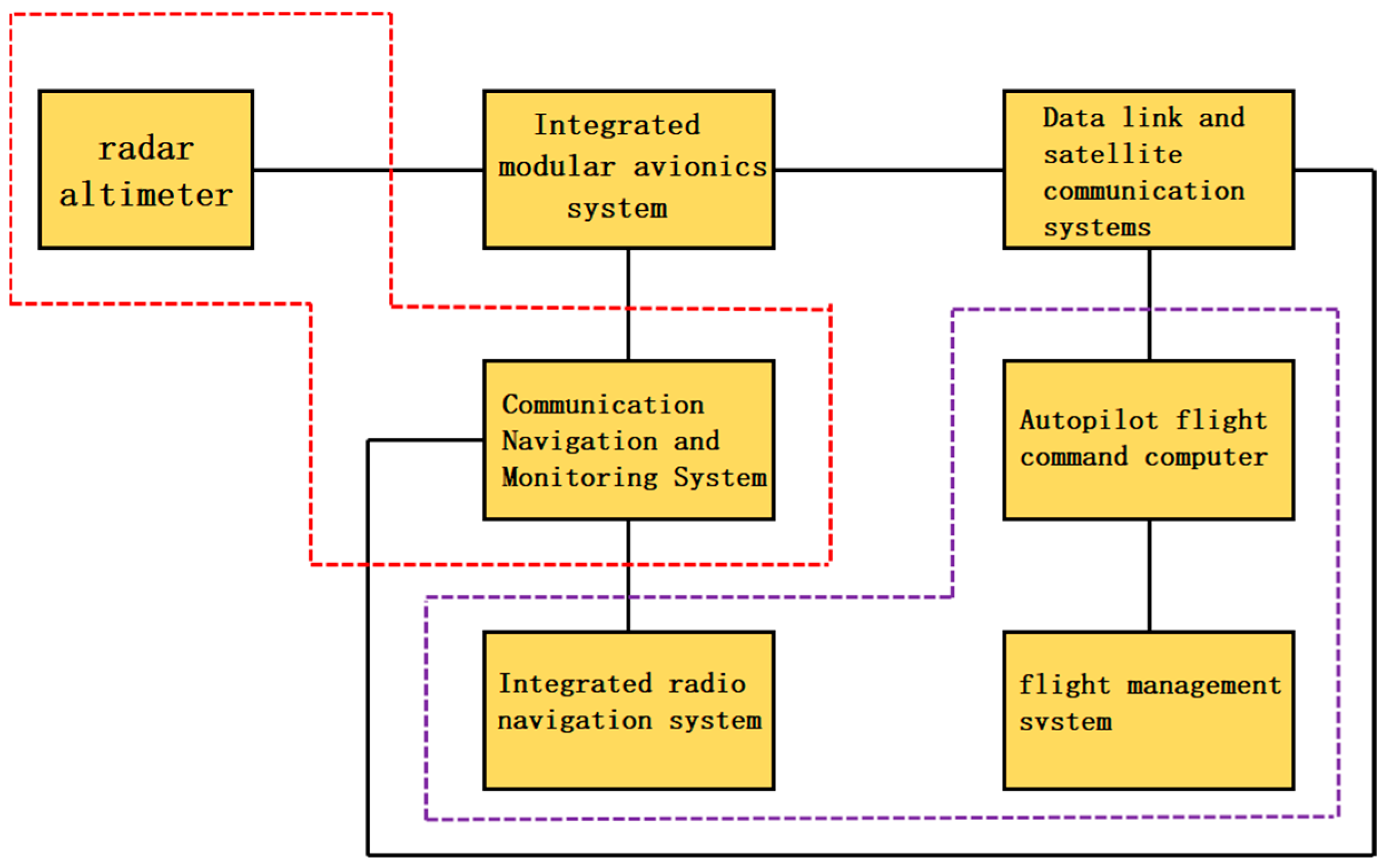
The ATM consists of different subsystems, such as the flight management system, communication, navigation and surveillance system, in-flight entertainment system, etc., and there may exist certain dependency relationships between the subsystems, i.e., the failure of a subsystem by an attack may lead to the damage of other subsystems with which it has a dependency relationship, e.g., the failure of Mode S transponders by an attack may lead to damage of the TCAS and the communication, navigation and surveillance system, which may lead to the damage of the flight management system. For example, the failure of Mode S transponders will lead to the damage of the TCAS, communication, navigation and monitoring system, and then lead to the damage of the flight management system, which will eventually lead to the damage of the autopilot flight command computer and the damage of the autopilot function of the airplane. Therefore, a network cascade failure model based on dynamic dependency groups is proposed to be used to analyze the process of impact propagation after a cyberattack.
The analysis model is described as follows. As shown in Figure 10, it is proposed to consider a network composed of certain subsystems in an ATM system as nodes and connectivity relationships as edges, with the nodes in the dashed box forming a dependency group, and the nodes in the group depending on each other. When a node in the dependency group fails, the remaining nodes are impacted to a certain extent, and the intensity of the impact is controlled by the decoupling coefficient α, i.e., each edge of each of the remaining nodes is retained with a probability of α, and deleted with a probability of 1-α. When α → 1, the coupling strength of the nodes in the dependency group is the weakest, and the failure of one node cannot cause any impact on the rest of the nodes in the group; whereas when α → 0, the coupling strength of the nodes in the dependency group is the strongest, and the failure of a single node can cause all the nodes in the group to be damaged. By adjusting the parameter α, the dependency strength of different subsystems in the avionics network can be described.
Network cascade failure is triggered by attacking certain nodes in the ATM system; the attacked nodes and their connections will be removed from the network altogether, which, in turn, leads to fragmentation of the network. In the network, the nodes that can connect to the giant branch are considered functional nodes, and the rest of the nodes are considered failed nodes. Due to a certain degree of dependency between nodes within the dynamic dependency group, the failure of a node in the network causes two kinds of impacts:
(1)
Out-of-group impact, the failure of a node causes network fragmentation, which, in turn, leads to the failure of some nodes outside the group that cannot connect to the network mega branch through that node;
(2)
In-group impact: the rest of the nodes in the dependency group in which the failed node is located are damaged and each of its connected edges is deleted with probability 1 − α, i.e., it is retained with probability α.
When a node fails, the out-group influence causes the failure to be able to propagate across the dependency group, thus extending the failure to a wider range, while the in-group influence causes the remaining nodes within the group to have their edges damaged, thus causing more nodes within the group to be damaged. Under the alternating effects of these two influences, cascading failures occur on the network.

7. Conclusions

In this paper, we successfully proposed a cyber threat entity recognition method for ATM based on TCFLTformer. The method combines a convolutional neural network, planarized representation, and Lattice Transformer model to effectively recognize cyber threat entities in ATM. We compared the proposed method with other popular cyber threat entity recognition methods in our experiments. The experimental results show that our method performs well in terms of accuracy and recall, proving its effectiveness in cyber threat entity recognition in ATM. In summary, the TCFLTformer cyber threat entity recognition method for ATM proposed in this paper has better performance and practicality and provides an effective solution for ATM cyber threat entity recognition.
There are some shortcomings in this study that require further research and improvement. First, the datasets used in this study are small in size and contain only a limited number of ATM cyber threat entities. Future research can consider expanding the size of the datasets to improve the generalization ability and robustness of the model. In addition, other large-scale deep learning models can be used for ATM cyber threat entity recognition, such as GPT [40] and RWKV [41], and future research can consider applying these models to ATM cyber threat entity recognition for comparison and analysis.

Author Contributions

Conceptualization, C.L. and Z.W.; methodology, C.L.; software, C.L.; validation, J.T., P.L. and Y.Y.; formal analysis, B.W.; investigation, Z.W.; resources, J.T.; data curation, C.L.; writing—original draft preparation, C.L.; writing—review and editing, C.L.; visualization, J.T.; supervision, P.L.; project administration, B.W. All authors have read and agreed to the published version of the manuscript.

Funding

This work was supported in part by the National Natural Science Foundation of China under Grant No. 61671465 which the funder is Buhong Wang, and in part by the China Postdoctoral Science Foundation under Grant No. 2021M692502, and the funder is Buhong Wang, who is the professor at the Air Force Engineering University.

Data Availability Statement

All the data used to support this study were reserved by the Air Force Engineering University School of Information and Navigation under license and cannot therefore be made freely available. Requests for access to these data should be made to [email protected].

Conflicts of Interest

The authors declare that there is no conflict of interest regarding the publication of this paper.

Appendix A

Table A1. The source of our datasets.
Source NameWebsite
NASAhttps://www.nasa.gov/ (accessed on 3 May 2021)
SESARhttps://www.geosamples.org/ (accessed on 3 May 2021)
FAAhttps://www.faa.gov/ (accessed on 3 May 2021)
EASAhttps://www.easa.europa.eu/en (accessed on 3 May 2021)
Microsoft Securityhttps://www.microsoft.com/en-us/security (accessed on 3 May 2021)
Naked Securityhttps://nakedsecurity.sophos.com/ (accessed on 3 May 2021)
Quick Heal Antivirus Bloghttps://blogs.quickheal.com/ (accessed on 3 May 2021)
Infosecurity Magazine–Information Security and IT Securityhttp://www.infosecurity-magazine.com/ (accessed on 3 May 2021)

References

  1. Pinto Neto, E.C.; Baum, D.M.; Almeida, J.R.D., Jr.; Camargo, J.B., Jr.; Cugnasca, P.S. Deep Learning in Air Traffic Management (ATM): A Survey on Applications, Opportunities, and Open Challenges. Aerospace 2023, 10, 358. [Google Scholar] [CrossRef]
  2. Post, J. The Next Generation Air Transportation System of the United States: Vision, Accomplishments, and Future Directions. Engineering 2021, 7, 427–430. [Google Scholar] [CrossRef]
  3. Bolic’, T.; Ravenhill, P. SESAR: The Past, Present, and Future of European Air Traffic Management Research. Engineering 2021, 7, 448–451. [Google Scholar] [CrossRef]
  4. International Threat Report Portugal Q1 2021. Available online: https://seguranca-informatica.pt/threat-report-portugal-q1-2021/ (accessed on 3 May 2021).
  5. Check Point Blog-Checkpoint’s Cyber Security Report 2021. Available online: https://blog.checkpoint.com/2021/06/14/ransomware-attacks-continue-to-surge-hitting-a-93-increase-year-over-year/ (accessed on 23 February 2022).
  6. Khandker, S.; Turtiainen, H.; Costin, A.; Hämäläinen, T. Cybersecurity attacks on software logic and error handling within ADS-B implementations: Systematic testing of resilience and countermeasures. IEEE Trans. Aerosp. Electron. Syst. 2021, 58, 2702–2719. [Google Scholar] [CrossRef]
  7. Ji, S.; Pan, S.; Cambria, E.; Marttinen, P.; Philip, S.Y. A survey on knowledge graphs: Representation, acquisition, and applications. IEEE Trans. Neural Netw. Learn. Syst. 2021, 33, 494–514. [Google Scholar] [CrossRef] [PubMed]
  8. Hogan, A.; Blomqvist, E.; Cochez, M.; d’Amato, C.; Melo, G.D.; Gutierrez, C.; Kirrane, S.; Gayo, J.E.L.; Navigli, R.; Neumaier, S.; et al. Knowledge graphs. ACM Comput. Surv. 2021, 54, 1–37. [Google Scholar] [CrossRef]
  9. Li, Z.; Liu, H.; Zhang, Z.; Liu, T.; Xiong, N.N. Learning knowledge graph embedding with heterogeneous relation attention networks. IEEE Trans. Neural Netw. Learn. Syst. 2021, 33, 3961–3973. [Google Scholar] [CrossRef]
  10. Chen, X.; Jia, S.; Xiang, Y. A review: Knowledge reasoning over knowledge graph. Expert Syst. Appl. 2020, 141, 112948. [Google Scholar] [CrossRef]
  11. Li, J.; Sun, A.; Han, J.; Li, C. A survey on deep learning for named entity recognition. IEEE Trans. Knowl. Data Eng. 2020, 34, 50–70. [Google Scholar] [CrossRef] [Green Version]
  12. Eddy, S.R. Hidden markov models. Curr. Opin. Struct. Biol. 1996, 6, 361–365. [Google Scholar] [CrossRef]
  13. Quinlan, J.R. Induction of decision trees. Mach. Learn. 1986, 1, 81–106. [Google Scholar] [CrossRef] [Green Version]
  14. Kapur, J.N. Maximum-Entropy Models in Science and Engineering; John Wiley & Sons: Hoboken, NJ, USA, 1989. [Google Scholar]
  15. Hearst, M.A.; Dumais, S.T.; Osuna, E.; Platt, J.; Scholkopf, B. Support vector machines. IEEE Intell. Syst. Their Appl. 1998, 13, 18–28. [Google Scholar] [CrossRef] [Green Version]
  16. Lafferty, J.; McCallum, A.; Pereira, F.C.N. Conditional random fields: Probabilistic models for segmenting and labeling sequence data. In Proceedings of the 18th International Conference on Machine Learning, Williamstown, MA, USA, 28 June–1 July 2001; pp. 282–289. [Google Scholar]
  17. McNamee, P.; Mayfield, J. Entity extraction without language-specific resources. In Proceedings of the 6th Conference on Natural Language Learning (CoNLL-2002), Taipei, Taiwan, 2002. [Google Scholar]
  18. McCallum, A.; Li, W. Early results for named entity recognition with conditional random fields, feature induction and web-enhanced lexicons. In Proceedings of the 7th conference on Natural language learning at HLT-NAACL, Edmonton, AB, Canada, 31 May–1 June 2003. [Google Scholar]
  19. Liu, X.; Chen, H.; Xia, W. Overview of named entity recognition. J. Contemp. Educ. Res. 2022, 6, 65–68. [Google Scholar] [CrossRef]
  20. Cao, Y.; Zhou, Y.; Shen, F.; Li, Z.X. Research on Named Entity Recognition of Chinese Electronic Medical Records Based on CNN-CRF. J. Chongqing Univ. Posts Telecommun. 2019, 6, 869–875. [Google Scholar]
  21. Kong, J.; Zhang, L.; Jiang, M.; Liu, T. Incorporating Multi-Level CNN and Attention Mechanism for Chinese Clinical Named Entity Recognition. J. Biomed. Inform. 2021, 116, 103737. [Google Scholar] [CrossRef]
  22. Peng, J.; Fang, Y.; Huang, C.; Liu, L.; Huang, Z. Cyber security named entity recognition based on deep active learning. J. Sichuan Univ. 2019, 56, 457–462. [Google Scholar]
  23. Li, T.; Guo, Y.; Ju, A. Knowledge triple extraction in cybersecurity with adversarial active learning. J. Commun. 2020, 41, 80–91. [Google Scholar]
  24. Yan, H.; Deng, B.; Li, X.; Qiu, X. TENER: Adapting Transformer Encoder for Named Entity Recognition. arXiv 2019, arXiv:1911.04474. [Google Scholar]
  25. Li, B.; Kang, X.; Zhang, H.; Wang, Y.; Chen, Y.; Bai, F. Named Entity Recognition of Chinese Electronic Medical Records Using Transformer-CRF. Comput. Eng. Appl. 2020, 56, 153–159. [Google Scholar]
  26. Zhang, X.; Li, Y.; Wang, D. Named Entity Recognition Based on ERNIE. Intell. Comput. Appl. 2020, 10, 21–26. [Google Scholar]
  27. Shen, T.; Yu, L.; Jin, L. Research on Chinese Entity Recognition Based on BERT-BILSTM-CRF Model. J. Qiqihar Univ. 2022, 38, 26–32. [Google Scholar]
  28. Guo, B.; Zhang, C.; Liu, J.; Ma, X. Improving text classification with weighted word embeddings via a multi-channel TextCNN model. Neurocomputing 2019, 363, 366–374. [Google Scholar] [CrossRef]
  29. Li, X.; Yan, H.; Qiu, X.; Huang, X. FLAT: Chinese NER using flat-lattice transformer. arXiv 2020, arXiv:2004.11795. [Google Scholar]
  30. Vaswani, A.; Shazeer, N.; Parmar, N.; Uszkoreit, J.; Jones, L.; Gomez, A.N.; Kaiser, Ł.; Polosukhin, I. Attention is all you need. Adv. Neural Inf. Process. Syst. 2017, 30, 5998–6008. [Google Scholar]
  31. Sidorov, G.; Velasquez, F.; Stamatatos, E.; Gelbukh, A.; Chanona-Hernández, L. Syntactic n-grams as machine learning features for natural language processing. Expert Syst. Appl. 2014, 41, 853–860. [Google Scholar] [CrossRef]
  32. Kenter, T.; Borisov, A.; De Rijke, M. Siamese cbow: Optimizing word embeddings for sentence representations. arXiv 2016, arXiv:1606.04640. [Google Scholar]
  33. Lin, Y.; Wang, C.; Song, H.; Li, Y. Multi-head self-attention transformation networks for aspect-based sentiment analysis. IEEE Access 2021, 9, 8762–8770. [Google Scholar] [CrossRef]
  34. Feng, J.; Li, Z.; Zhang, D. Bridge Detection Text Named Entity Recognition Based on Hidden Markov Model. Traffic World 2020, 8, 32–33. [Google Scholar]
  35. Chauhan, V.K.; Dahiya, K.; Sharma, A. Problem formulations and solvers in linear SVM: A review. Artif. Intell. Rev. 2019, 52, 803–855. [Google Scholar] [CrossRef]
  36. Webb, G.I.; Keogh, E.; Miikkulainen, R. Naïve Bayes. Encycl. Mach. Learn. 2010, 15, 713–714. [Google Scholar]
  37. Yang, H.; Li, L.; Yang, R. Recognition Model of Electronic Medical Record Named Entity Based on Bidirectional LSTM Neural Network. Chin. Tissue Eng. Res. 2018, 22, 3237–3242. [Google Scholar]
  38. Chao, Z.; Hai-Chun, S.; Ye-Bai, S. Chinese Event Trigger Word Extraction Using ERNIE-BIGRU-CRF. In Proceedings of the 2021 China Automation Congress (CAC) (IEEE), Beijing, China, 22–24 October 2021; pp. 3792–3797. [Google Scholar]
  39. Meng, F.; Yang, S.; Wang, J.; Xia, L.; Liu, H. Creating knowledge graph of electric power equipment faults based on BERT-BiLSTM-CRF model. J. Electr. Eng. Technol. 2022, 17, 2507–2516. [Google Scholar] [CrossRef]
  40. Zhang, C.; Zhang, C.; Zheng, S.; Qiao, Y.; Li, C.; Zhang, M.; Dam, S.K.; Thwal, C.M.; Tun, Y.L.; Huy, L.L. A Complete Survey on Generative AI (AIGC): Is ChatGPT from GPT-4 to GPT-5 All You Need? arXiv 2023, arXiv:2303.11717. [Google Scholar]
  41. Peng, B.; Alcaide, E.; Anthony, Q.; Albalak, A.; Arcadinho, S.; Cao, H.; Chen, X.; Chung, M.; Grella, M.; GV, K.K.; et al. RWKV: Reinventing RNNs for the Transformer Era. arXiv 2023, arXiv:2305.13048. [Google Scholar]
Figure 1. Air Traffic Management System.
Aerospace 10 00697 g001
Figure 2. ATM cyber threat knowledge graph construction process.
Aerospace 10 00697 g002
Figure 3. Principle of ATM cyber threat entity recognition.
Aerospace 10 00697 g003
Figure 4. The overall architecture of TCFLTformer.
Aerospace 10 00697 g004
Figure 5. The feature learning process of the TCFLTformer.
Aerospace 10 00697 g005
Figure 6. The input of the multibranch prediction head.
Aerospace 10 00697 g006
Figure 7. Comparison of experimental results.
Aerospace 10 00697 g007
Figure 8. Comparison of experimental results of four types of threat entities.
Aerospace 10 00697 g008aAerospace 10 00697 g008b
Figure 9. ATM cyber threat word clouds.
Aerospace 10 00697 g009
Figure 10. A network composed of certain subsystems in the ATM system.
Aerospace 10 00697 g010
Table 1. The source of our datasets.
Source NameNumber of Articles
NASA265
SESAR226
FAA249
EASA159
Microsoft Security265
Naked Security265
Quick Heal Antivirus Blog117
InfoSecurity Magazine—Information Security and IT Security258
Others267
Count2071
Table 2. TCFLTformer model training process.
For each epoch loop:
    For each batch loop:
    (1)
Parameter initialization;
    (2)
Token character-level n-grams for word vectorization;
    (3)
TextCNN extracts entity feature vectors;
    (4)
The word vector and the feature matrix of the TextCNN output are input into Flat-Lattice Transformer;
    (5)
The Flat-Lattice Transformer model passes backward to automatically learn to extract features;
    (6)
The CRF layer calculates the global likelihood probability of the sequence;
    (7)
Update parameters;
    Ending the batch loop;
Ending the epoch loop;
Table 3. The analysis of datasets.
DatasetsData TypeSentencesTokensTags
Train9499348,57911,004
Validation135749,8031373
Test271499,5883343
Count13,570497,97015,720
Table 4. The analysis of named entities.
Tag NameCountRatio
Malware699144.47%
Hash337821.49%
URL436327.75%
IP9886.28%
Table 5. Accuracy from 20 experiments.
Model NameAverage-ValueMax-ValueMin-Value
BiLSTM-CRF92.36292.60691.847
Transformer-CRF92.95193.02292.883
ERNIE-BiGRU-CRF92.83393.07992.794
BERT-BiLSTM-CRF93.10493.16592.935
TCFLTformer93.31293.38293.184
Table 6. Experimental results of different models.
Model NameAccMacroaveragingMicroaveraging
PRFPRF
SVM77.2052.1052.9052.5053.5054.4653.98
Naive Bayes74.8068.4059.7063.7568.8066.4067.58
BiLSTM-CRF92.3667.3852.2158.8383.7580.6282.16
Transformer-CRF92.9571.7858.0464.1886.1782.0784.07
ERNIE-BiGRU-CRF92.8369.9866.3968.1484.7085.1884.94
BERT-BiLSTM-CRF93.1072.6165.2368.7286.4784.0785.25
TCFLTformer93.3174.2963.6368.5588.4583.6886.00
Table 7. The detailed statistics of datasets.
DatasetsTypeTrain/103Validation/103Test/103
MASA 1char2169.9-172.6
sentence46.4-4.4
token74.7-6.2
Boson 2char424.852.151.7
sentence8.81.11.1
token18.02.22.2
Table 8. Experimental results on MASA and Boson.
Model NameMASABoson
PRFPRF
BiLSTM-CRF94.57194.23394.40281.81282.024 81.918
Transformer-CRF95.95196.78596.36687.18690.17488.655
ERNIE-BiGRU-CRF97.42197.67497.54788.65391.68390.143
BERT-BiLSTM-CRF97.98597.96297.97388.52991.70190.087
TCFLTformer98.51298.52598.51889.99392.09491.031
Disclaimer/Publisher’s Note: The statements, opinions and data contained in all publications are solely those of the individual author(s) and contributor(s) and not of MDPI and/or the editor(s). MDPI and/or the editor(s) disclaim responsibility for any injury to people or property resulting from any ideas, methods, instructions or products referred to in the content.

