
Exploring the Performance Boundaries of a Small Reconfigurable Multi-Mission UAV through Multidisciplinary Analysis


Abstract
1. Introduction
1.1. Background
1.2. Research Objectives
2. Materials and Methods
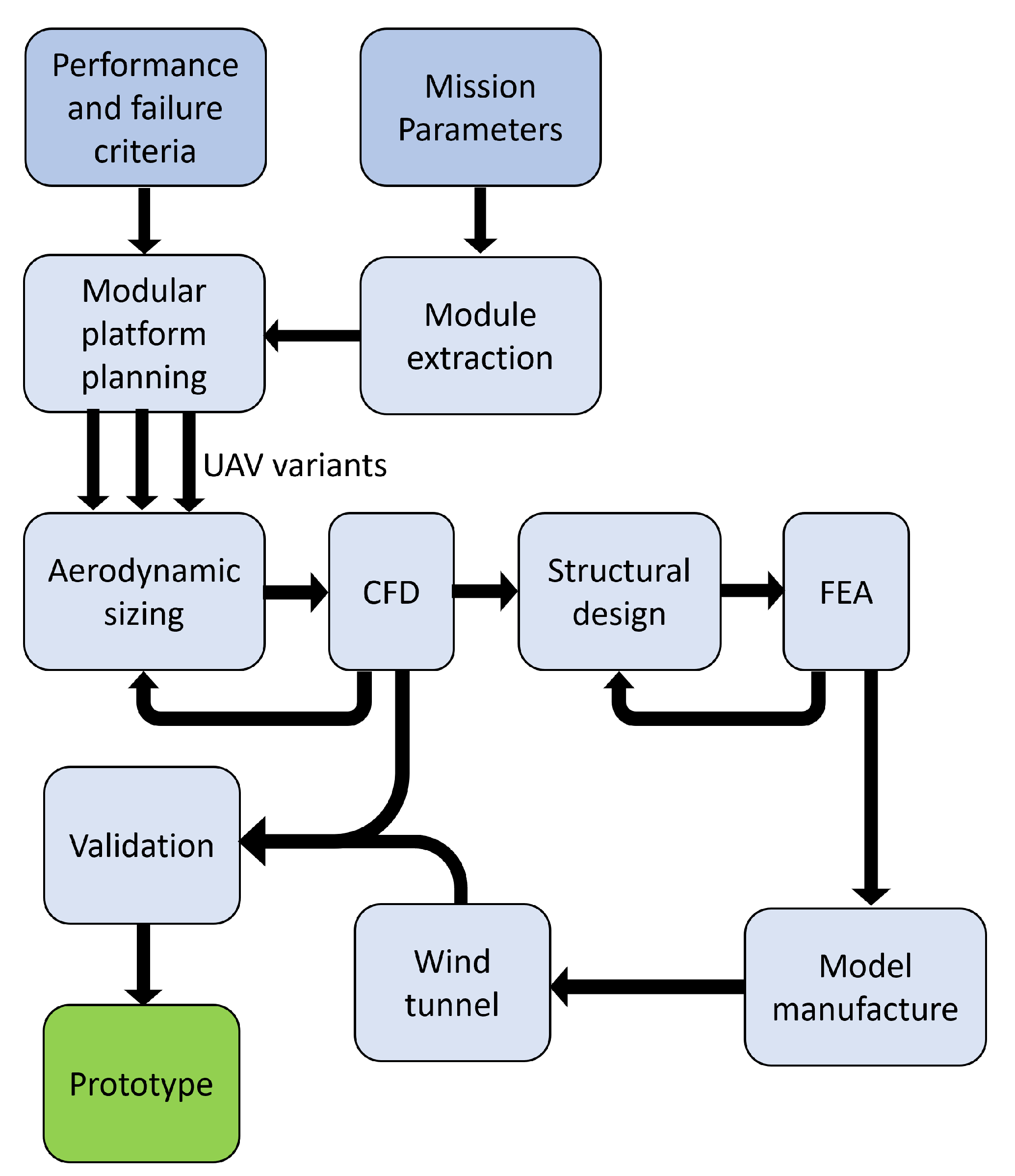
2.1. Multidisciplinary Approach
2.2. Computational Fluid Dynamics Studies
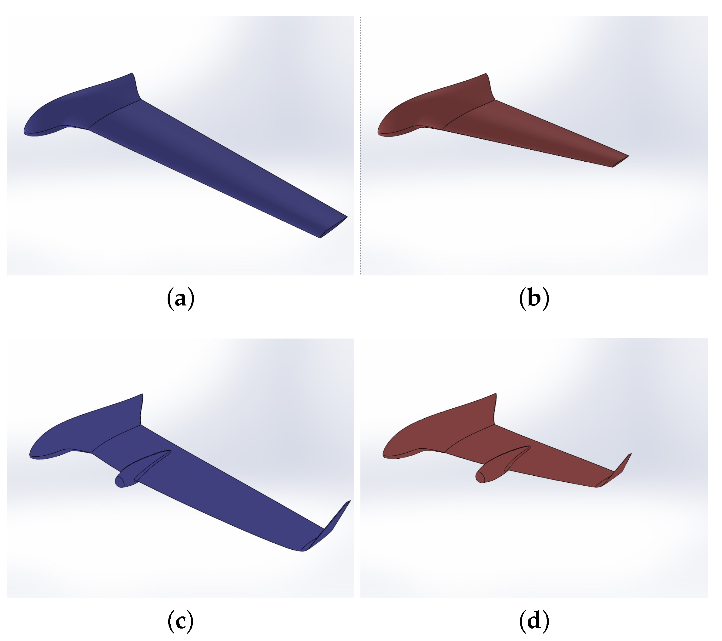
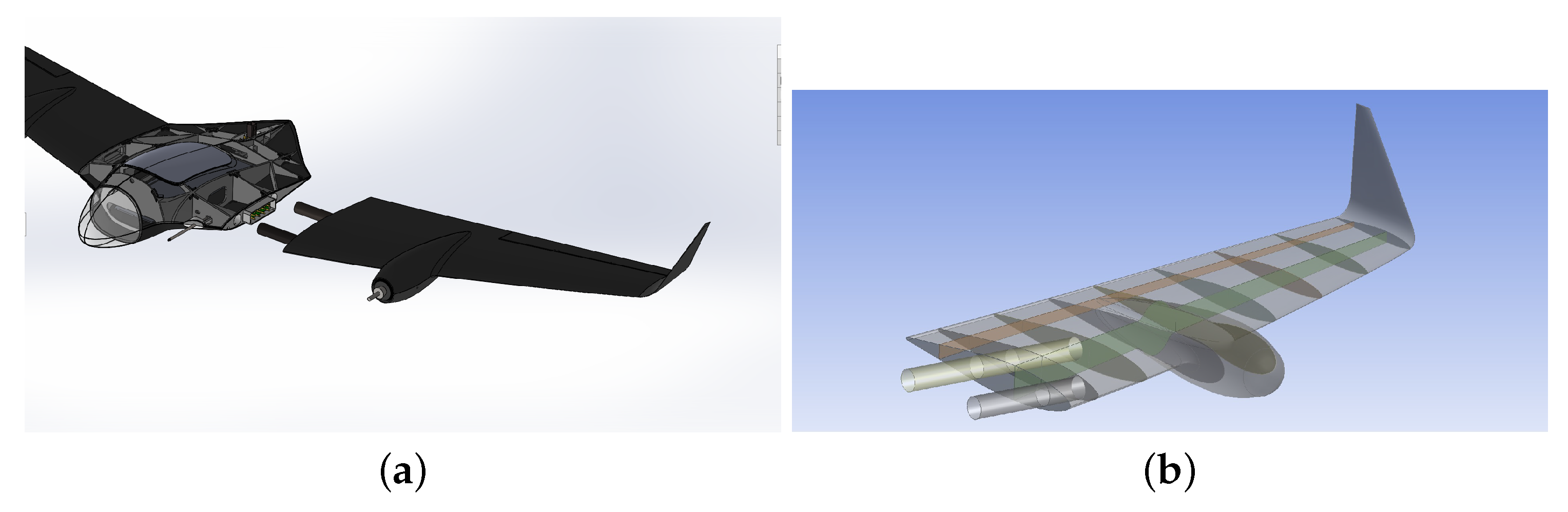
2.2.1. CFD Geometries
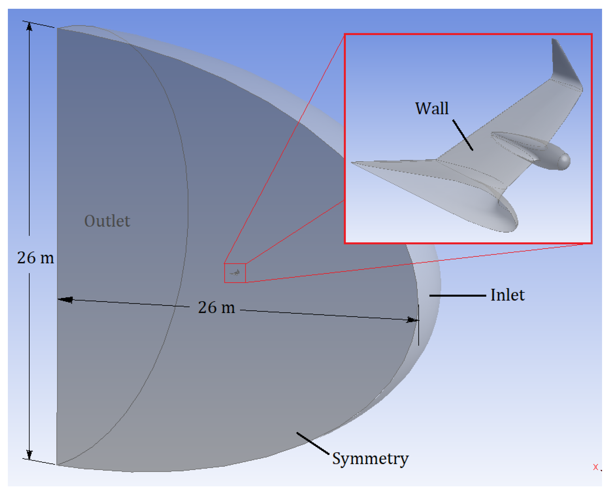
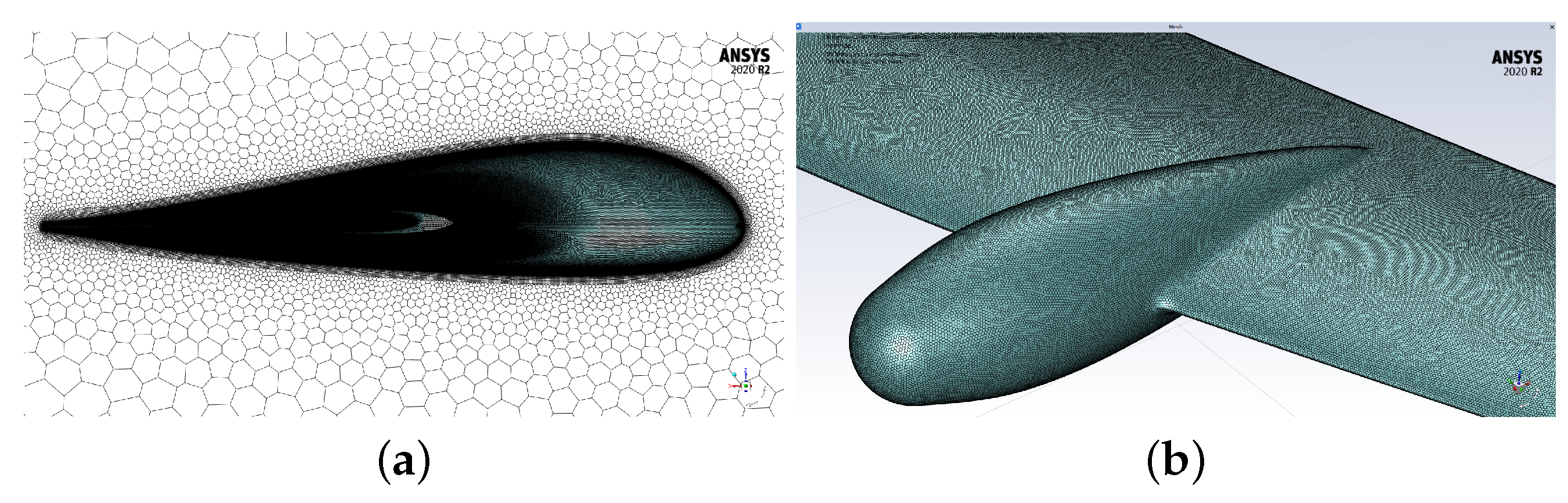
2.2.2. CFD Meshes
2.2.3. CFD Turbulence Method and Flow Conditions
2.3. Finite Element Analysis Studies
2.3.1. FEA Geometry
2.3.2. Material Properties
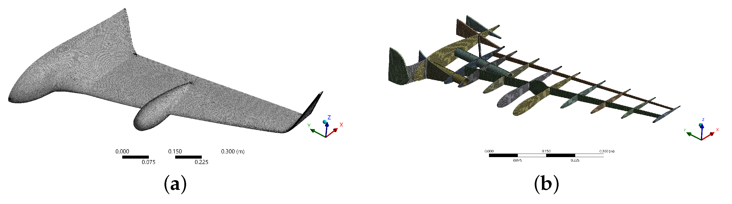
2.3.3. FEA Meshes
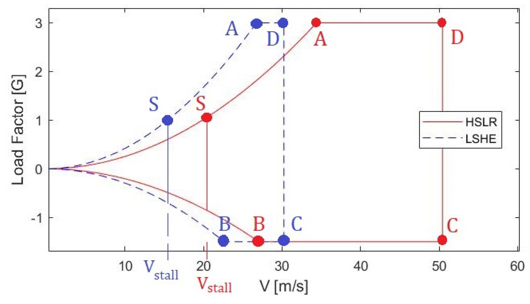
2.3.4. Load and Boundary Conditions
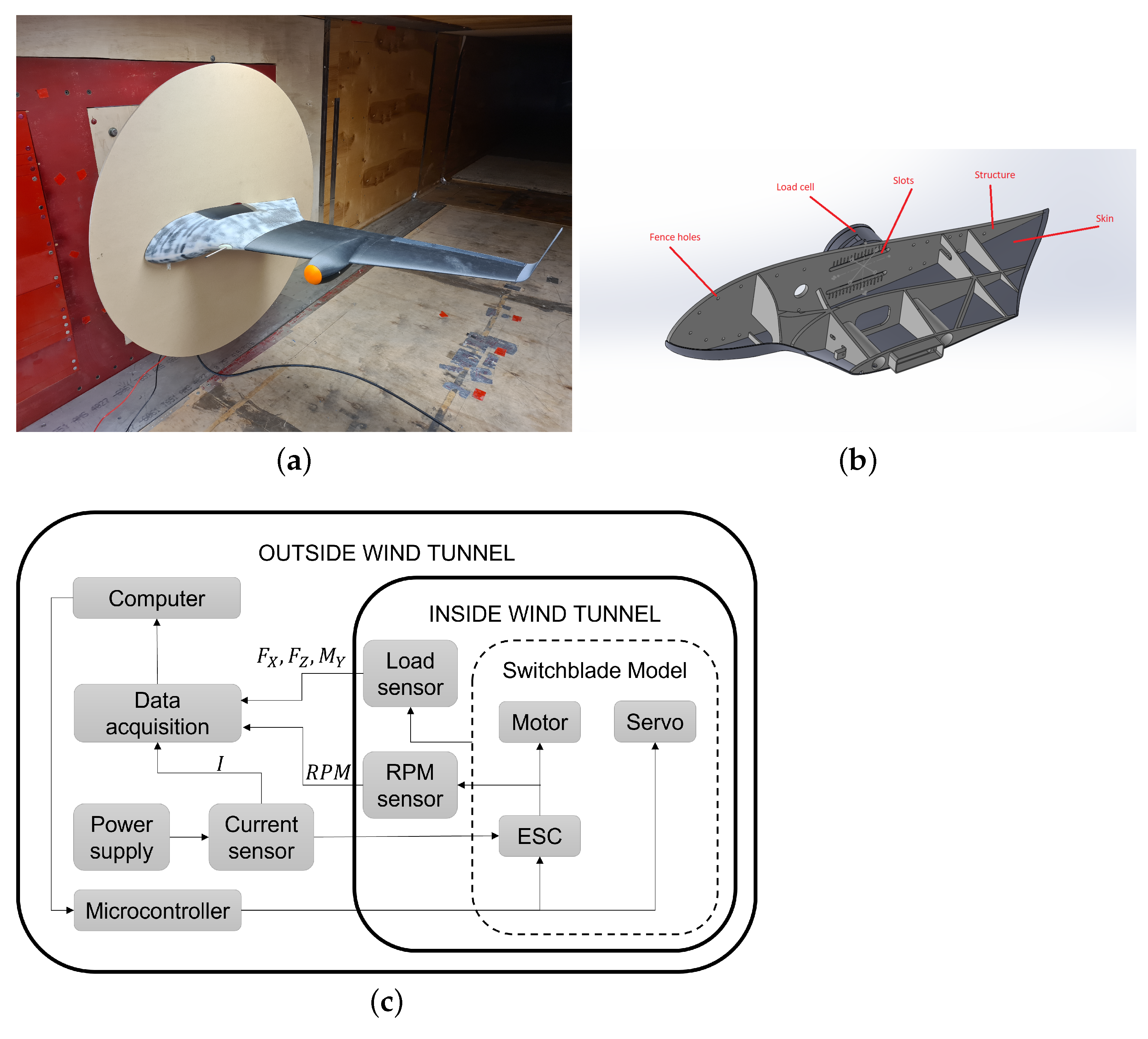
2.4. Wind Tunnel Experiments
2.4.1. Aerodynamic Center Finding Procedure
2.4.2. Lift, Drag, and Moment Measurements
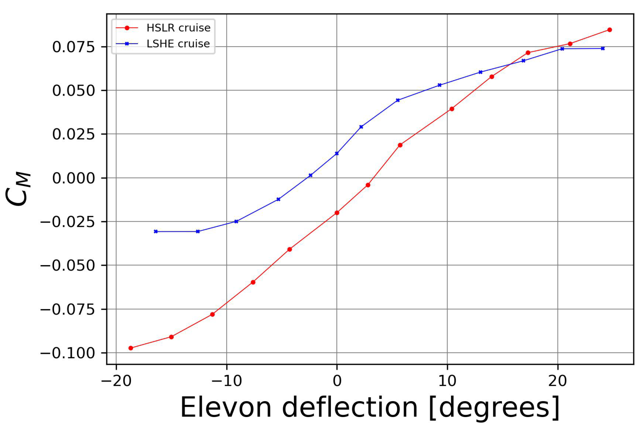
2.4.3. Elevon Effectiveness and Trimming Procedure
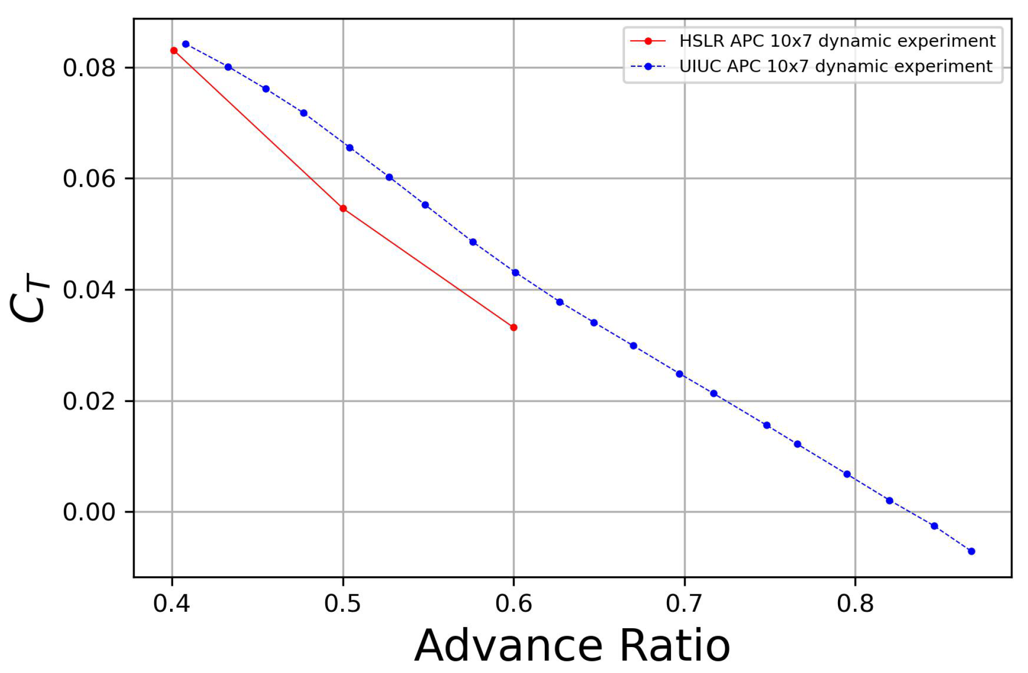
2.4.4. Thrust Experiment
3. Results and Discussion
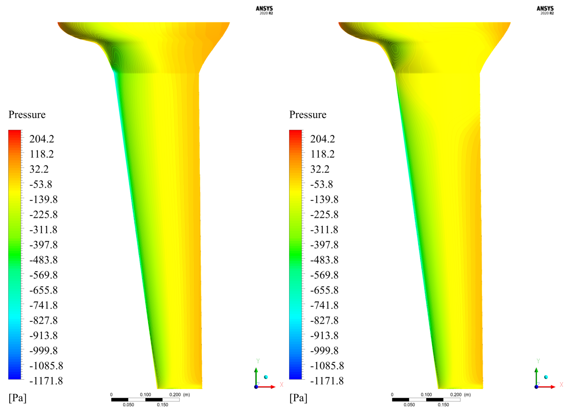
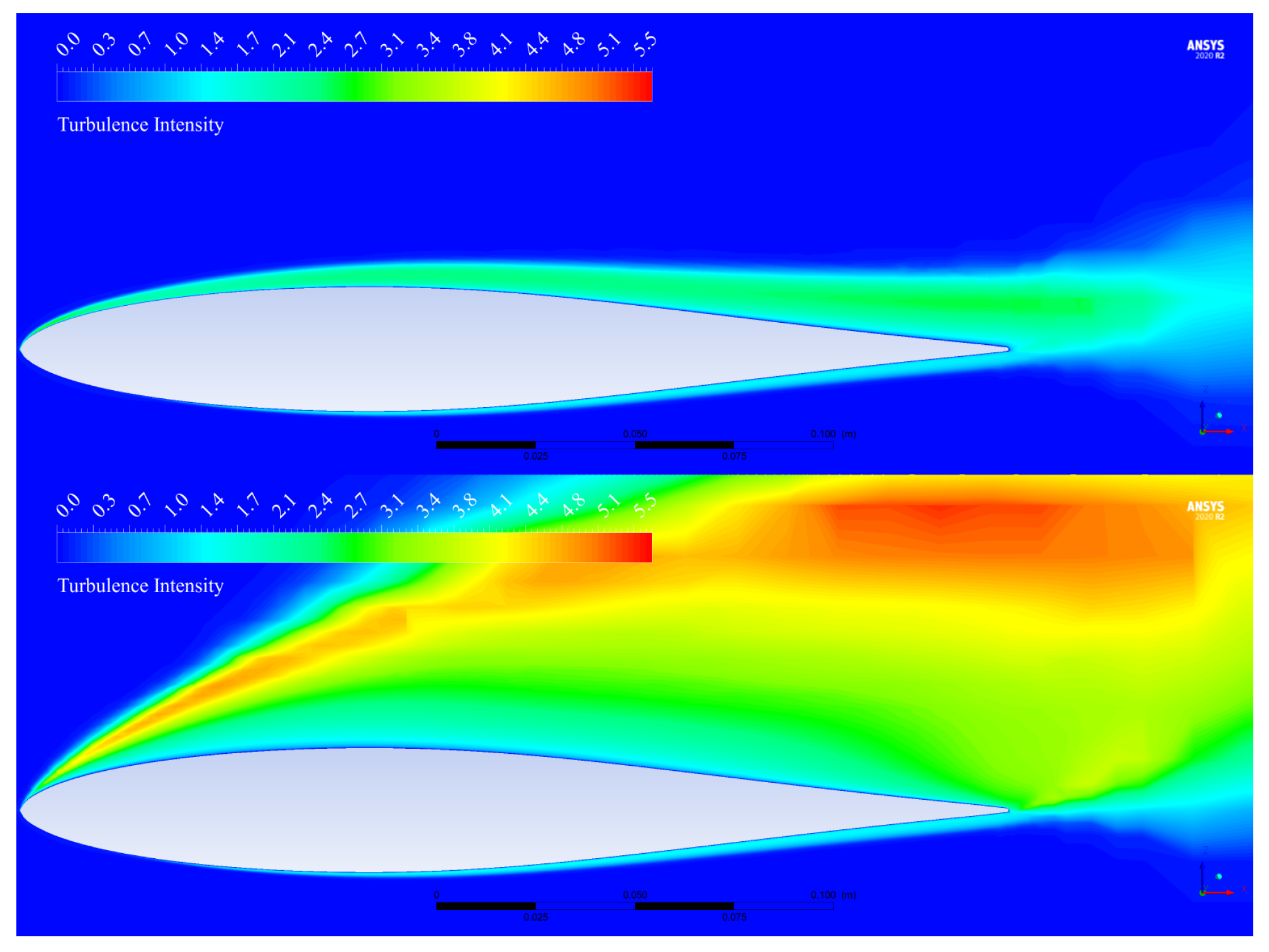
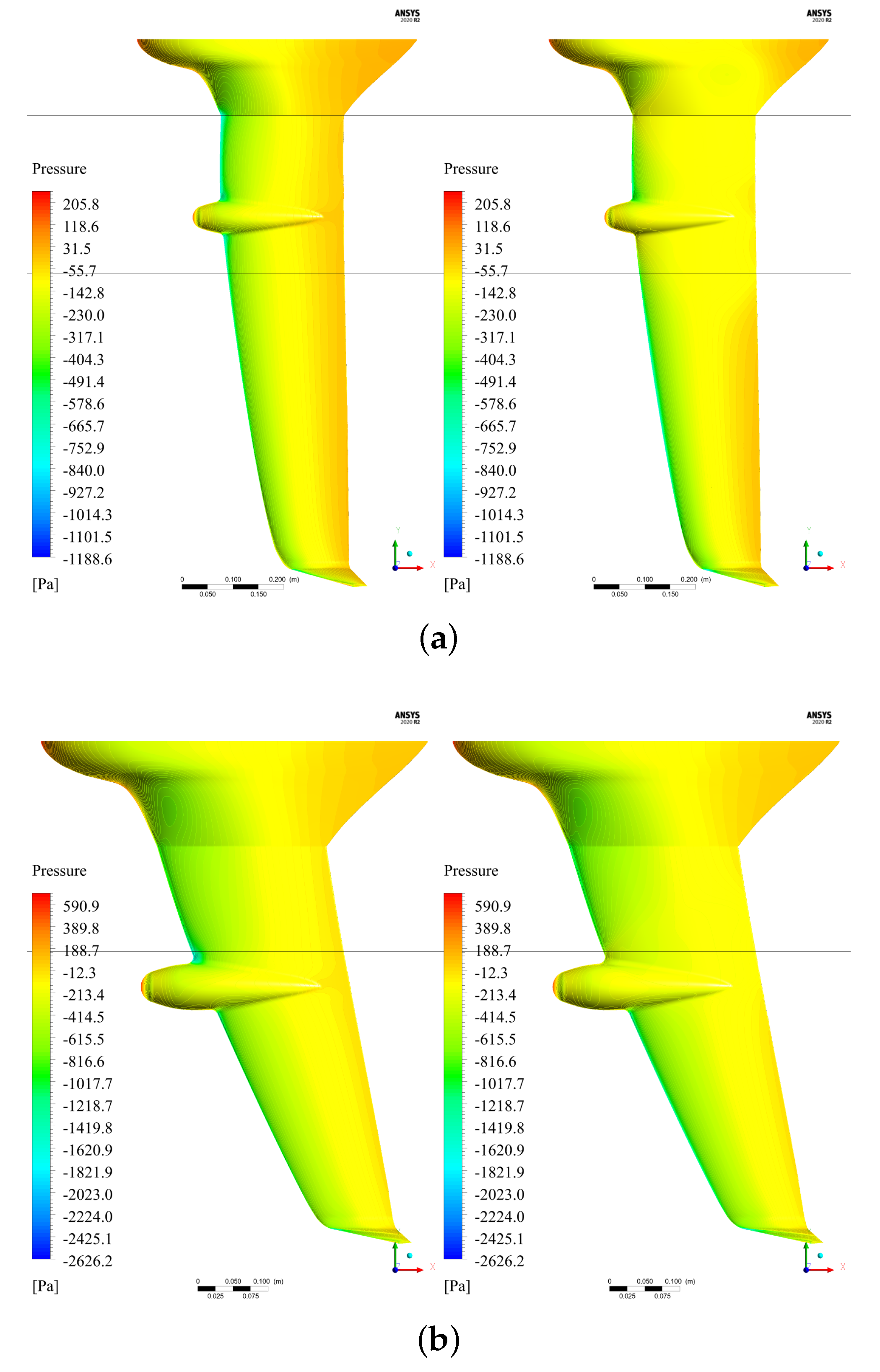
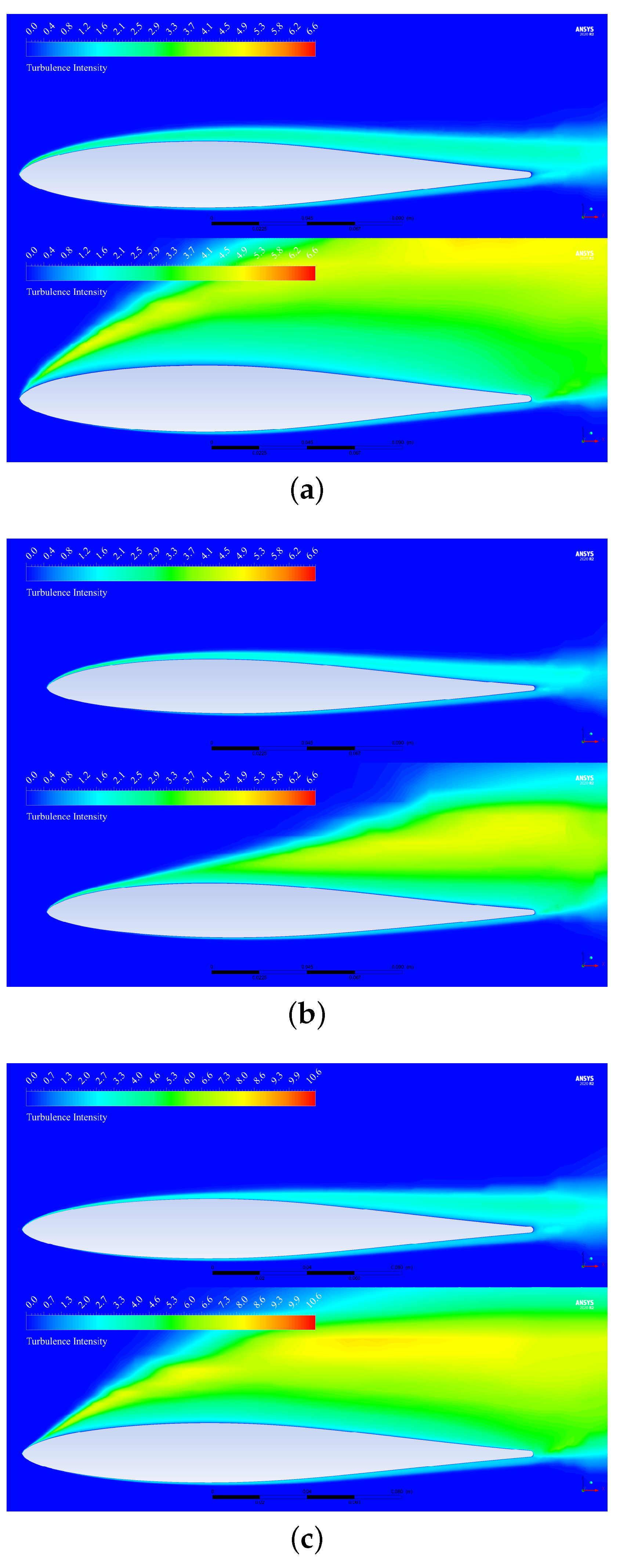
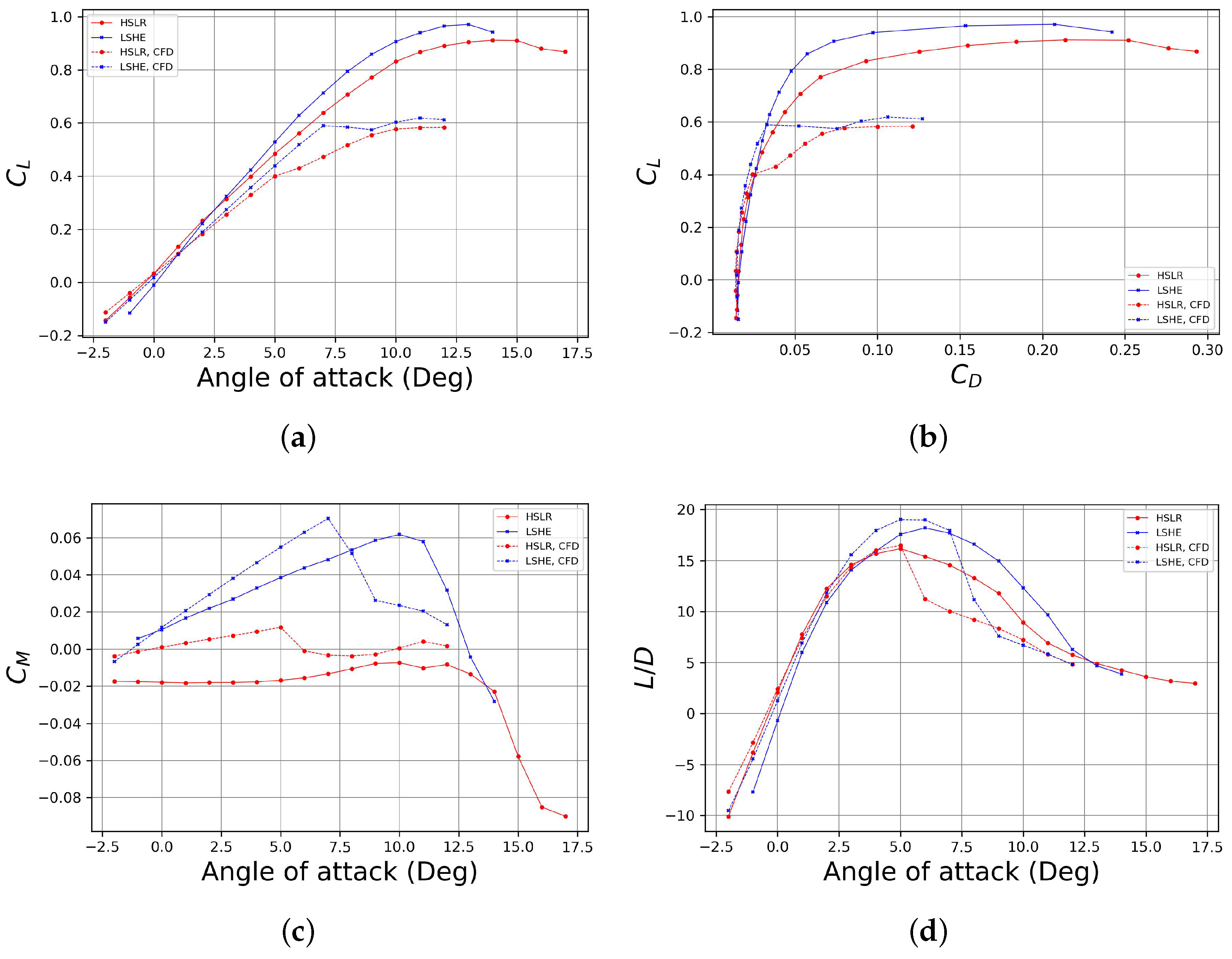
3.1. CFD Aerodynamic Results
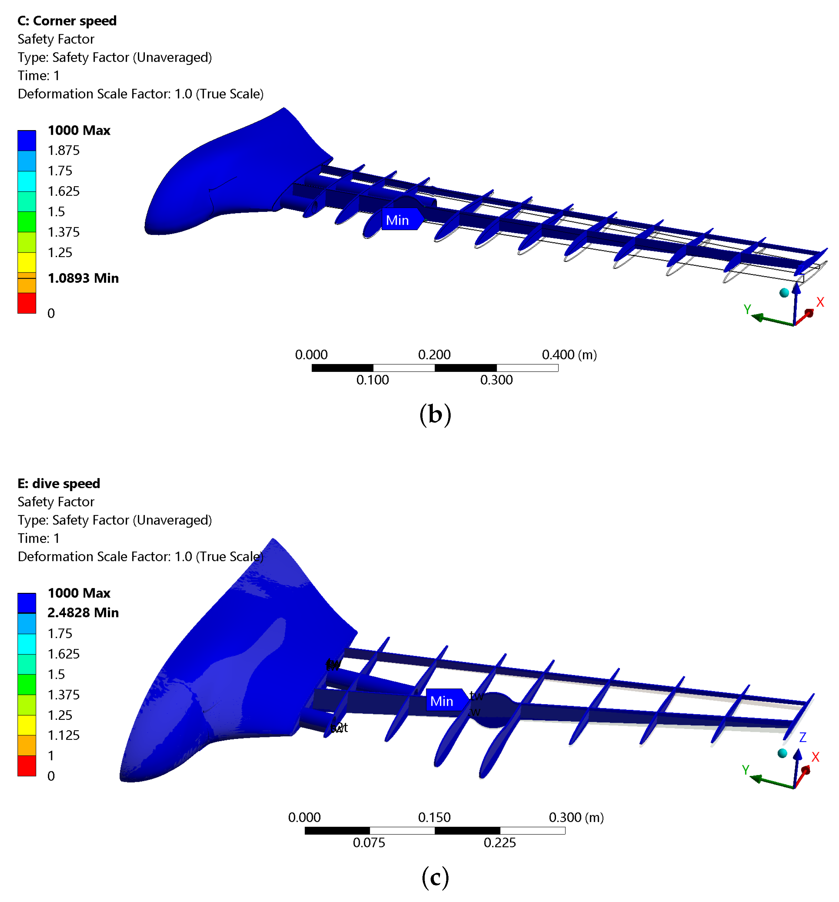
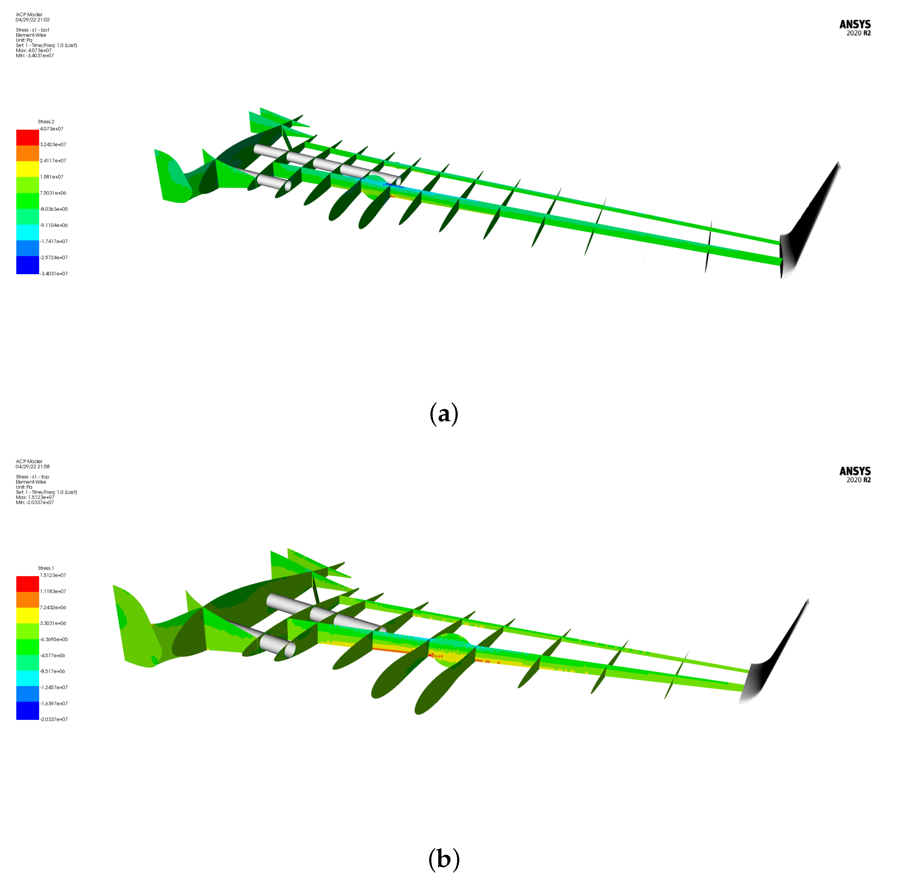
3.2. FEA Results
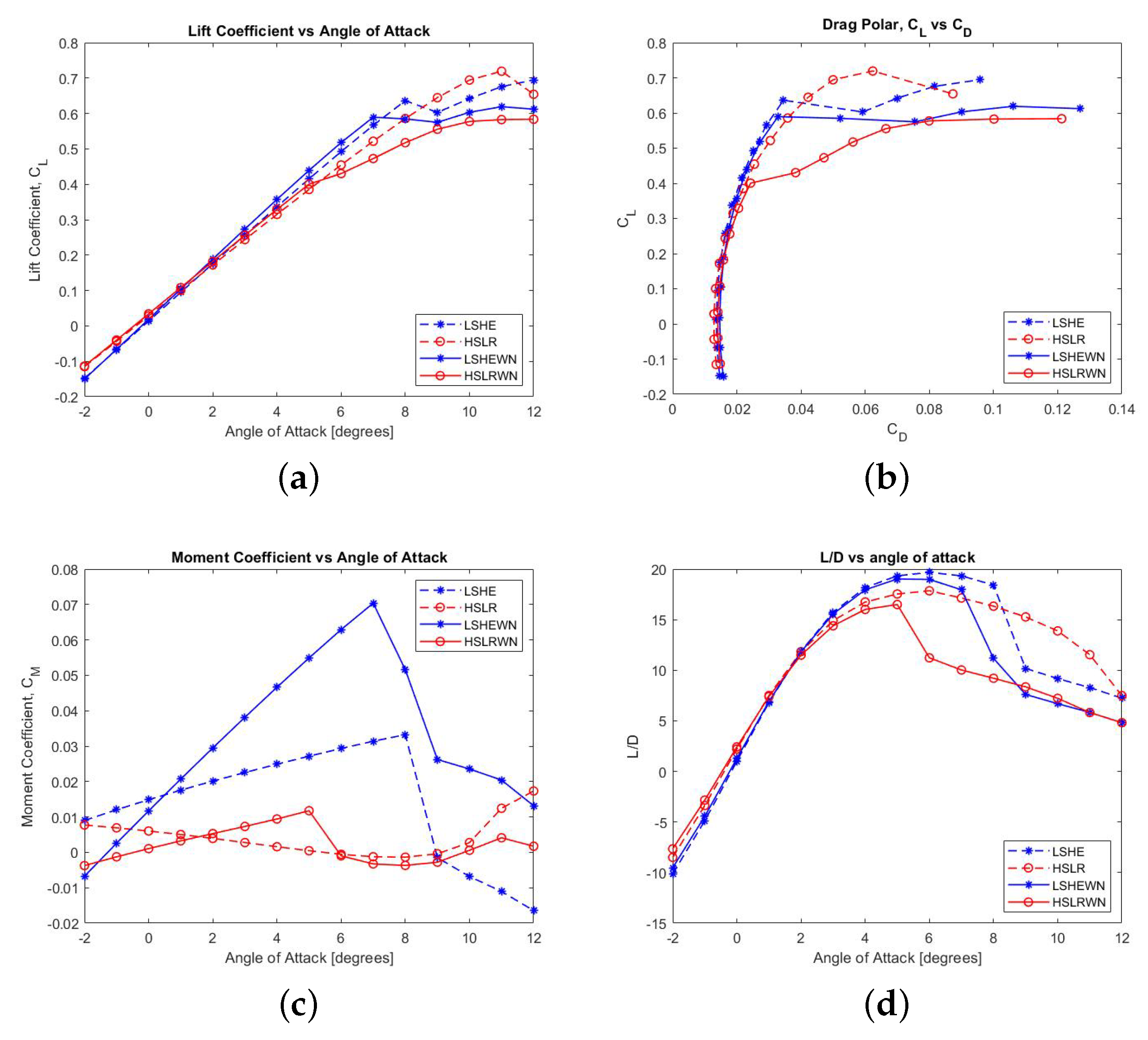
3.3. Experimental Results
4. Conclusions
Author Contributions
Funding
Data Availability Statement
Acknowledgments
Conflicts of Interest
Abbreviations
| UAV | Unmanned Aerial Vehicle |
| UAS | Unmanned Aerial System |
| CFD | Computational Fluid Dynamics |
| RANS | Reynolds-Averaged Navier–Stokes |
| URANS | Unsteady Reynolds-Averaged Navier–Stokes |
| DES | Detached Eddy Simulation |
| FEA | Finite Element Analysis |
| RVE | Representative Volume Element |
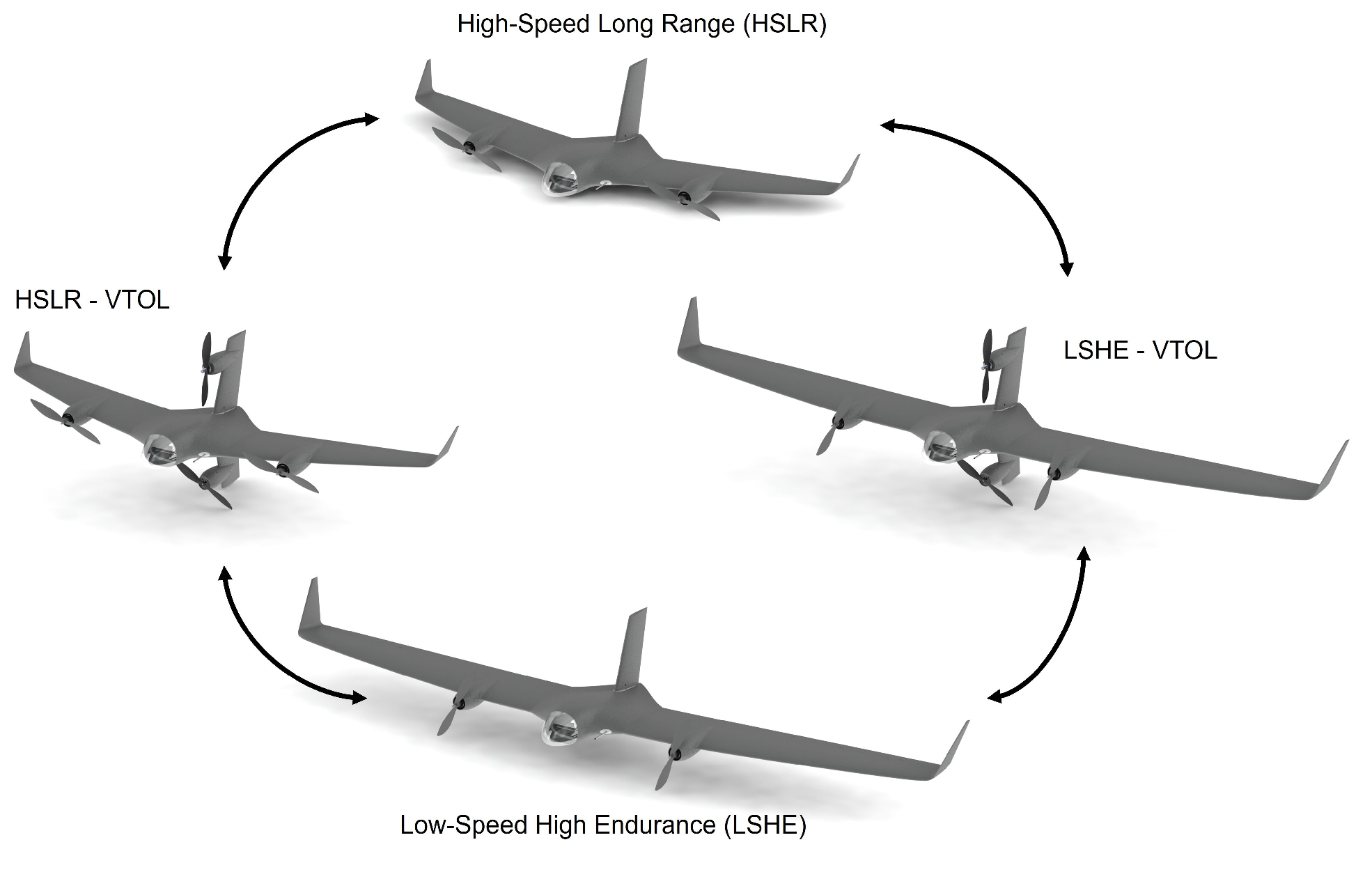
| HSLR | High-Speed Long-Range |
| LSHE | Low-Speed High-Endurance |
| Angle-of-Attack | |
| DoF | Degrees of Freedom |
References
- Goh, C.Y.; Leow, C.Y.; Nordin, R. Energy Efficiency of Unmanned Aerial Vehicle with Reconfigurable Intelligent Surfaces: A Comparative Study. Drones 2023, 7, 98. [Google Scholar] [CrossRef]
- Yang, Z.; Yu, X.; Dedman, S.; Rosso, M.; Zhu, J.; Yang, J.; Xia, Y.; Tian, Y.; Zhang, G.; Wang, J. UAV remote sensing applications in marine monitoring: Knowledge visualization and review. Sci. Total. Environ. 2022, 838, 155939. [Google Scholar] [CrossRef]
- Mozaffari, M.; Saad, W.; Bennis, M.; Nam, Y.H.; Debbah, M. A Tutorial on UAVs for Wireless Networks: Applications, Challenges, and Open Problems. IEEE Commun. Surv. Tutor. 2019, 21, 2334–2360. [Google Scholar] [CrossRef]
- Zhao, C.; Shi, K.; Tang, Y.; Xiao, J.; He, N. Multi-Group Tracking Control for MASs of UAV with a Novel Event-Triggered Scheme. Drones 2023, 7, 474. [Google Scholar] [CrossRef]
- Lyu, M.; Zhao, Y.; Huang, C.; Huang, H. Unmanned Aerial Vehicles for Search and Rescue: A Survey. Remote. Sens. 2023, 15, 3266. [Google Scholar] [CrossRef]
- Hu, P.; Zhang, R.; Yang, J.; Chen, L. Development Status and Key Technologies of Plant Protection UAVs in China: A Review. Drones 2022, 6, 354. [Google Scholar] [CrossRef]
- Kaitao, M.; Wu, Q.; Xu, J.; Chen, W.; Feng, Z.; Schober, R.; Swindlehurst, A. UAV-Enabled Integrated Sensing and Communication: Opportunities and Challenges. IEEE Wirel. Commun. 2023, 1–9. [Google Scholar] [CrossRef]
- Su, J.; Zhu, X.; Li, S.; Chen, W.H. AI meets UAVs: A survey on AI empowered UAV perception systems for precision agriculture. Neurocomputing 2023, 518, 242–270. [Google Scholar] [CrossRef]
- Da Silva Ferreira, M.A.; Begazo, M.F.T.; Lopes, G.C.; de Oliveira, A.F.; Colombini, E.L.; da Silva Simões, A. Drone Reconfigurable Architecture (DRA): A Multipurpose Modular Architecture for Unmanned Aerial Vehicles (UAVs). J. Intell. Robot. Syst. 2020, 99, 517–534. [Google Scholar] [CrossRef]
- Chowdhury, S.; Maldonado, V.; Tong, W.; Messac, A. New Modular Product-Platform-Planning Approach to Design Macroscale Reconfigurable Unmanned Aerial Vehicles. J. Aircr. 2016, 53, 309–322. [Google Scholar] [CrossRef]
- Pate, D.J.; Patterson, M.D.; German, B.J. Optimizing Families of Reconfigurable Aircraft for Multiple Missions. J. Aircr. 2012, 49, 1988–2000. [Google Scholar] [CrossRef]
- Maldonado, V.; Santos, D.; Wilt, M.; Ramirez, D.; Shoemaker, J.; Ayele, W.; Beeson, B.; Lisby, B.; Zamora, J.; Antu, C. ‘Switchblade’: Wide-Mission Performance Design of a Multi-Variant Unmanned Aerial System. In Proceedings of the AIAA Scitech 2021 Forum, Virtual Event, 11–15 January 2021. [Google Scholar] [CrossRef]
- Santos, D.; Ramirez, D.; Rogers, J.; Zamora, J.; Rezende, A.; Maldonado, V. Full-Cycle Design and Analysis of the Switchblade Reconfigurable Unmanned Aerial System. In Proceedings of the AIAA Aviation 2022 Forum, Chicago, IL, USA, 27 June–1 July 2022. [Google Scholar] [CrossRef]
- El Adawy, M.; Abdelhalim, E.H.; Mahmoud, M.; Ahmed Abo zeid, M.; Mohamed, I.H.; Othman, M.M.; ElGamal, G.S.; ElShabasy, Y.H. Design and fabrication of a fixed-wing Unmanned Aerial Vehicle (UAV). Ain Shams Eng. J. 2023, 14, 102094. [Google Scholar] [CrossRef]
- Ayele, W.; Maldonado, V. Conceptual Design of a Robotic Ground-Aerial Vehicle with an Aeroelastic Wing Model for Mars Planetary Exploration. Aerospace 2023, 10, 404. [Google Scholar] [CrossRef]
- Chu, L.; Gu, F.; Du, X.; He, Y. Design and analysis of morphing wing UAV adopted to harsh environment based on “Frigate bird”. In Proceedings of the 2022 IEEE International Conference on Robotics and Biomimetics (ROBIO), Jinghong, China, 5–9 December 2022; pp. 1295–1300. [Google Scholar] [CrossRef]
- Elelwi, M.; Kuitche, M.; Botez, R.; Dao, T. Comparison and analyses of a variable span-morphing of the tapered wing with a varying sweep angle. Aeronaut. J. 2020, 124, 1146–1169. [Google Scholar] [CrossRef]
- Gatto, A. Development of a morphing UAV for optimal multi-segment mission performance. Aeronaut. J. 2023, 127, 1320–1352. [Google Scholar] [CrossRef]
- Goetzendorf-Grabowski, T.; Tarnowski, A.; Figat, M.; Mieloszyk, J.; Hernik, B. Lightweight unmanned aerial vehicle for emergency medical service—Synthesis of the layout. Proc. Inst. Mech. Eng. Part J. Aerosp. Eng. 2021, 235, 5–21. [Google Scholar] [CrossRef]
- Kim, T.; Jeaong, H.; Kim, S.; Kim, I.; Kim, S.; Suk, J.; Shin, H.S. Design and Flight Testing of the Ducted-fan UAV Flight Array System. J. Intellegent Robot. Syst. 2023, 107. [Google Scholar] [CrossRef]
- Lu, D.; Xiong, C.; Zhou, H.; Lyu, C.; Hu, R.; Yu, C.; Zeng, Z.; Lian, L. Design, fabrication, and characterization of a multimodal hybrid aerial underwater vehicle. Ocean. Eng. 2021, 219, 108324. [Google Scholar] [CrossRef]
- Lyu, C.; Lu, D.; Xiong, C.; Hu, R.; Jin, Y.; Wang, J.; Zeng, Z.; Lian, L. Toward a gliding hybrid aerial underwater vehicle: Design, fabrication, and experiments. J. Field Robot. 2022, 39, 543–556. [Google Scholar] [CrossRef]
- Savastano, E.; Perez-Sanchez, V.; Arrue, B.; Ollero, A. High-Performance Morphing Wing for Large-Scale Bio-Inspired Unmanned Aerial Vehicles. IEEE Robot. Autom. Lett. 2022, 7, 8076–8083. [Google Scholar] [CrossRef]
- Wong, S.M.; Ho, H.W.; Abdullah, M.Z. Design and Fabrication of a Dual Rotor-Embedded Wing Vertical Take-Off and Landing Unmanned Aerial Vehicle. Unmanned Syst. 2021, 9, 45–63. [Google Scholar] [CrossRef]
- Wang, Y.C.; Chen, T.; Yeh, Y.L. Advanced 3D printing technologies for the aircraft industry: A fuzzy systematic approach for assessing the critical factors. Int. J. Adv. Manuf. Technol. 2019, 105, 4059–4069. [Google Scholar] [CrossRef]
- Liu, X.; Li, D.; Qi, P.; Qiao, W.; Shang, Y.; Jiao, Z. A local resistance coefficient model of aircraft hydraulics bent pipe using laser powder bed fusion additive manufacturing. Exp. Therm. Fluid Sci. 2023, 147, 110961. [Google Scholar] [CrossRef]
- Kobenko, S.; Dejus, D.; Jātnieks, J.; Pazars, D.; Glaskova-Kuzmina, T. Structural Integrity of the Aircraft Interior Spare Parts Produced by Additive Manufacturing. Polymers 2022, 14, 1538. [Google Scholar] [CrossRef] [PubMed]
- Zhu, W. Models for wind tunnel tests based on additive manufacturing technology. Prog. Aerosp. Sci. 2019, 110, 100541. [Google Scholar] [CrossRef]
- Raza, A.; Farhan, S.; Nasir, S.; Salamat, S. Applicability of 3D Printed Fighter Aircraft Model for Subsonic Wind Tunnel. In Proceedings of the 2021 International Bhurban Conference on Applied Sciences and Technologies (IBCAST), Islamabad, Pakistan, 12–16 January 2021; pp. 730–735. [Google Scholar] [CrossRef]
- Bardera, R.; Rodríguez-Sevillano, Á.; Barderas, E.B.; Casati, M.J.. Rapid prototyping by additive manufacturing of a bioinspired micro-RPA morphing model for a wind tunnel test campaign. In Proceedings of the AIAA AVIATION 2022 Forum, Chicago, IL, USA, 27 June–1 July 2022. [Google Scholar] [CrossRef]
- Tsushima, N.; Saitoh, K.; Nakakita, K. Structural and aeroelastic characteristics of wing model for transonic flutter wind tunnel test fabricated by additive manufacturing with AlSi10Mg alloys. Aerosp. Sci. Technol. 2023, 140, 108476. [Google Scholar] [CrossRef]
- Taylor, R.M.; Niakin, B.; Lira, N.; Sabine, G.; Lee, J.; Conklin, C.; Advirkar, S. Design Optimization, Fabrication, and Testing of a 3D Printed Aircraft Structure Using Fused Deposition Modeling. In Proceedings of the AIAA Scitech 2020 Forum, Orlando, FL, USA, 6–10 January 2020. [Google Scholar] [CrossRef]
- Skawinski, I.; Goetzendorf-Grabowski, T. FDM 3D printing method utility assessment in small RC aircraft design. Aircr. Eng. Aerosp. Technol. 2019, 91, 865–872. [Google Scholar] [CrossRef]
- Mani, M.; Dorgan, A.J. A Perspective on the State of Aerospace Computational Fluid Dynamics Technology. Annu. Rev. Fluid Mech. 2023, 55, 431–457. [Google Scholar] [CrossRef]
- Ma, Z.; Tang, Z.; Wang, R.; Yu, Z. Research Progress in Numerical Simulation of Aircraft Wing Flow Field. J. Phys. Conf. Ser. 2023, 2457, 012047. [Google Scholar] [CrossRef]
- Le Clainche, S.; Ferrer, E.; Gibson, S.; Cross, E.; Parente, A.; Vinuesa, R. Improving aircraft performance using machine learning: A review. Aerosp. Sci. Technol. 2023, 138, 108354. [Google Scholar] [CrossRef]
- García-Gutiérrez, A.; Gonzalo, J.; López, D.; Delgado, A. Advances in CFD Modeling of Urban Wind Applied to Aerial Mobility. Fluids 2022, 7, 246. [Google Scholar] [CrossRef]
- Panagiotou, P.; Yakinthos, K. Aerodynamic efficiency and performance enhancement of fixed-wing UAVs. Aerosp. Sci. Technol. 2020, 99, 105575. [Google Scholar] [CrossRef]
- Tormalm, M.; Schmidt, S. Computational Study of Static And Dynamic Vortical Flow over the Delta Wing SACCON Configuration Using the FOI Flow Solver Edge. In Proceedings of the 28th AIAA Applied Aerodynamics Conference, Chicago, IL, USA, 28 June–1 July 2010. [Google Scholar] [CrossRef]
- Sandoval, P.; Cornejo, P.; Tinapp, F. Evaluating the longitudinal stability of an UAV using a CFD-6DOF model. Aerosp. Sci. Technol. 2015, 43, 463–470. [Google Scholar] [CrossRef]
- Mumtaz, M.S.; Maqsood, A.; Sherbaz, S. Computational Modeling of Dynamic Stability Derivatives for Generic Airfoils. MATEC Web Conf. 2017, 95, 12006. [Google Scholar] [CrossRef]
- Greenblatt, D.; Williams, D.R. Flow Control for Unmanned Air Vehicles. Annu. Rev. Fluid Mech. 2022, 54, 383–412. [Google Scholar] [CrossRef]
- Kim, M.; Kim, S.; Kim, W.; Kim, C.; Kim, Y. Flow Control of Tiltrotor Unamnned-Aerial-Vehicle Airfoils Using Synthetic Jets. J. Aircr. 2011, 48, 1045–1057. [Google Scholar] [CrossRef]
- Bliamis, C.; Vlahostergios, Z.; Misirlis, D.; Yakinthos, K. Numerical Evaluation of Riblet Drag Reduction on a MALE UAV. Aerospace 2022, 9, 218. [Google Scholar] [CrossRef]
- Guiler, R.; Huebsch, W. Wind Tunnel Analysis of a Morphing Swept Wing Tailless Aircraft. In Proceedings of the 23rd AIAA Applied Aerodynamics Conference, Toronto, ON, Canada, 6–9 June 2005. [Google Scholar] [CrossRef]
- Goetten, F.; Finger, D.; Marino, M.; Bil, C.; Havermann, M.; Braun, C. A Review of Guidelines and Best Practices for Subsonic Aerodynamic Simulations Using RANS CFD. In Proceedings of the Asia Pacific International Symposium on Aerospace Technology, Gold Coast, Australia, 4–6 December 2019. [Google Scholar]
- Zore, K.; Shah, S.; Stokes, J.; Sasanapuri, B.; Sharkey, P. ANSYS CFD Study for High Lift Aircraft Configurations. In Proceedings of the 2018 Applied Aerodynamics Conference, Atlanta, GA, USA, 25–29 June 2018. [Google Scholar] [CrossRef]
- Menter, F.R.; Smirnov, P.E.; Liu, T.; Avancha, R. A One-Equation Local Correlation-Based Transition Model. Flow Turbul. Combust 2015, 95, 583–619. [Google Scholar] [CrossRef]
- Menter, F. Two-Equation Eddy-Viscosity Turbulence Models for Engineering Applications. AIAA J. 1994, 32, 8. [Google Scholar] [CrossRef]
- Vostruha, K.; Pelant, J. Perturbation Analysis of “k-ω” and “k-ϵ” Turbulent Models. Wall Functions. EPJ Web Conf. 2013, 45, 01097. [Google Scholar] [CrossRef]
- Rodriguez, S. Applied Computational Fluid Dynamics and Turbulence Modeling: Practical Tools, Tips and Techniques; Springer International Publishing: Berlin/Heidelberg, Germany, 2019. [Google Scholar]
- Gu, J.; Chen, P.; Su, L.; Li, K. A theoretical and experiemental assessment of 3D macroscopic failure criteria for predicting pure inter-fiber fracture of transversely isotropic UD composites. Compos. Struct. 2020, 259, 113466. [Google Scholar]
- Stratasys. Nylon 12 Carbon Fiber. 2015. Available online: https://www.stratasys.com/en/materials/materials-catalog/fdm-materials/Nylon-12/ (accessed on 6 June 2022).
- Chen, R.; Ramachandran, A.; Liu, C.; Chang, F.K.; Senesky, D. Tsai-Wu Analysis of a Thin-Walled 3D-Printed Polylactic Acid (PLA) Structural Bracket. In Proceedings of the 58th AIAA/ASCE/AHS/ASC Structures, Structural Dynamics, and Materials Conference, Grapevine, TX, USA, 9–13 January 2017. [Google Scholar] [CrossRef]
- Administration, F.A. Federal Aviation Regulations Part 23, § 23.337. 2023. Available online: https://www.govinfo.gov/app/details/CFR-2017-title14-vol1/CFR-2017-title14-vol1-sec23-337 (accessed on 4 May 2022).
- Raymer, D. Aircraft Design: A Conceptual Approach; American Institute of Aeronautics and Astronautics: Reston, VA, USA, 2012; pp. 203–205. [Google Scholar] [CrossRef]
- Evans, S.; Lardeau, S. Validation of a turbulence methodology using the SST k-ω model for adjoint calculation. In Proceedings of the 54th AIAA Aerospace Sciences Meeting, San Diego, CA, USA, 4–8 January 2016. [Google Scholar] [CrossRef]
- Spalart, P.R.; Rumsey, C.L. Effective Inflow Conditions for Turbulence Models in Aerodynamic Calculations. AIAA J. 2007, 45, 2544–2553. [Google Scholar] [CrossRef]
- Castillo, R.; Pol, S. Wind tunnel studies of wind turbine yaw and speed control effects on the wake trajectory and thrust stabilization. Renew. Energy 2022, 189, 726–733. [Google Scholar] [CrossRef]
- Maldonado, V.; Castillo, L.; Thormann, A.; Meneveau, C. The role of free stream turbulence with large integral scale on the aerodynamic performance of an experimental low Reynolds number S809 wind turbine blade. J. Wind. Eng. Ind. Aerodyn. 2015, 142, 246–257. [Google Scholar] [CrossRef]
- Brandt, J.; Selig, M. Propeller Performance Data at Low Reynolds Numbers. In Proceedings of the 49th AIAA Aerospace Sciences Meeting including the New Horizons Forum and Aerospace Exposition, Orlando, FL, USA, 4–7 January 2011. [Google Scholar] [CrossRef]
- Ananda, G. UIUC Propeller Database, Volume 1. 2015. Available online: https://m-selig.ae.illinois.edu/props/volume-1/propDB-volume-1.html (accessed on 15 October 2022).
- Traub, L.W. Range and Endurance Estimates for Battery-Powered Aircraft. J. Aircr. 2011, 48, 703–707. [Google Scholar] [CrossRef]


| Paper | Variant or Type | Manufacture | Wing Airfoil | Materials | Endurance | Cruise Speed | Range | L/D |
|---|---|---|---|---|---|---|---|---|
| Adawy [14] | Fixed wing | Laser cut, foam cutting | E423 | Balsawood Plywood Aluminum | 14.5 m/s | |||
| Ayele [15] | Inflatable wing | E180 | Polyurethane blade UV-sensitive woven material | 0.34 h | 158.21 m/s | 13.8 | ||
| Chu [16] | Max. Extension | 16 m/s | 21.5 | |||||
| Transition | N/A | 17 m/s | 19.9 | |||||
| Min. Extension | 18 m/s | 19 | ||||||
| Elelwi [17] | 100% span length | NACA 4412 | 51 m/s | 102 km | 23.76 | |||
| 125% span length | NACA 4412 | 51 m/s | 120 km | 26.5 | ||||
| 150% span length | NACA 4412 | 51 m/s | 130 km | 29 | ||||
| 175% span length | NACA 4412 | 51 m/s | 150 km | 32.35 | ||||
| Gatto [18] | Active twist control | Laser Cut | Variable | Balsawood Plywood Fiberglass | 18–25 m/s | 9.8–10.66 | ||
| Goetzendorf- Gabowski [19] | Fixed wing VTOL | S4062-095-87 | 1.5 h | 22 m/s | 14.3 | |||
| Kim [20] | Multi-UAV Array | Assembled Components | N/A | Various | 0.17 h | |||
| Individual UAV | Assembled Components | N/A | Various | 0.17 h | ||||
| Lu [21] | Air | Off-the-shelf Components | Carbon fiber | 31.5 m/s | 3.92 | |||
| Water | Off-the-shelf Components | Carbon fiber | Depth 50 m | |||||
| Lyu [22] | Air | Off-the-shelf Components | Composite | 0.17 h | ||||
| Water | Off-the-shelf Components | Composite | 0.37 h | 0.5 m/s | Depth 25 m | |||
| Santos | LSHE | 3D printed | E171/E330 | Nylon 12 CF | 1.8 h | 20.16 m/s | 131 km | 18.2 |
| HSLR | 3D printed | E171//E182 | Nylon 12 CF | 0.49 h | 33.62 m/s | 59 km | 16.2 | |
| Savastano [23] | Flapping wing | AS-6091 | Ultralight fabric | 11 m/s | 76 | |||
| Wong [24] | Fixed wing VTOL | Foam cutting | MH 78 | polystyrene woven glass fiber | 4 |
| Mission | Performance | Range | Cruise Mach | VTOL | Payload | Weight |
|---|---|---|---|---|---|---|
| Surveillance | LSHE | 200 km | 0.06 | No | Camera | 3.93 |
| Delivery | HSLR-VTOL | 100 km | 0.1 | Yes | Package | 4.66 |
| Inspection | LSHE-VTOL | 37 km | 0.06 | Yes, 30 min | Camera | 4.50 |
| UAV Variant | Location | Airfoil | Thickness, %c | Camber, %c | |
|---|---|---|---|---|---|
| LSHE | Root | Eppler 171 | 12.28 | 0 | 0.008 |
| LSHE | Tip | Eppler 330 | 11 | 2.1 | 0.01 |
| HSLR | Root | Eppler 171 | 12.28 | 0 | 0.008 |
| HSLR | Tip | Eppler 182 | 8.5 | 1.2 | 0.007 |
| UAV Geometry | S [m] | A | Span, b [m] | Sweep, | Taper Ratio, |
|---|---|---|---|---|---|
| LSHE | 0.476 | 9.7 | 2.15 | 7.8° | 0.53 |
| HSLR | 0.309 | 6.6 | 1.43 | 24° | 0.35 |
| LSHEWN | 0.488 | 9.5 | 2.15 | 7.8° | 0.53 |
| HSLRWN | 0.324 | 6.3 | 1.43 | 24° | 0.35 |
| Model | Cells | Nodes | Wall Faces | Quality | Face Size | Inflation |
|---|---|---|---|---|---|---|
| LSHE | 0.20 | 2 mm | 30 | |||
| HSLR | 0.11 | 1 mm | 30 | |||
| LSHEWN | 0.11 | 3 mm | 25 | |||
| HSLRWN | 0.19 | 1 mm | 25 |
| Aircraft Model | Target Size | Elements | Nodes | Min. Quality | Average Quality |
|---|---|---|---|---|---|
| LSHE | 3 mm | 180,647 | 157,269 | 0.041 | 0.893 |
| HSLR | 3 mm | 157,401 | 132,626 | 0.044 | 0.887 |
| Variant | Analysis Point | Airspeed [m/s] | Angle of Attack [] | |
|---|---|---|---|---|
| HSLR | A | 12.0 | 0.584 | |
| HSLR | D | 3.2 | 0.272 | |
| LSHE | A | 11.0 | 0.619 | |
| LSHE | D | 6.4 | 0.549 |
| Load Case | FoS | Spar [MPa] | [mm] | [N] | [N] | [N] | [N] |
|---|---|---|---|---|---|---|---|
| LSHE, corner | 1.09 | 40.7 | 25.4 | 2.53 | −65.51 | 129.6 | 132.4 |
| LSHE, dive | 1.16 | 38.2 | 24.2 | 5.05 | −71.57 | 143.4 | 132.4 |
| HSLR, corner | 2.61 | 14.3 | 8.3 | 2.60 | −70.50 | 139.0 | 130.8 |
| HSLR, dive | 2.48 | 15.1 | 8.8 | 1.40 | −65.58 | 131.1 | 130.8 |
| Variant | Flight Speed [m/s] | Endurance [h] | Range [km] |
|---|---|---|---|
| LSHE | 20.16 | 1.80 | 131 |
| HSLR | 33.62 | 0.49 | 59 |
Disclaimer/Publisher’s Note: The statements, opinions and data contained in all publications are solely those of the individual author(s) and contributor(s) and not of MDPI and/or the editor(s). MDPI and/or the editor(s) disclaim responsibility for any injury to people or property resulting from any ideas, methods, instructions or products referred to in the content. |
© 2023 by the authors. Licensee MDPI, Basel, Switzerland. This article is an open access article distributed under the terms and conditions of the Creative Commons Attribution (CC BY) license (https://creativecommons.org/licenses/by/4.0/).
Share and Cite
Santos, D.; Rogers, J.; De Rezende, A.; Maldonado, V. Exploring the Performance Boundaries of a Small Reconfigurable Multi-Mission UAV through Multidisciplinary Analysis. Aerospace 2023, 10, 684. https://doi.org/10.3390/aerospace10080684
Santos D, Rogers J, De Rezende A, Maldonado V. Exploring the Performance Boundaries of a Small Reconfigurable Multi-Mission UAV through Multidisciplinary Analysis. Aerospace. 2023; 10(8):684. https://doi.org/10.3390/aerospace10080684
Chicago/Turabian StyleSantos, Dioser, Jeremy Rogers, Armando De Rezende, and Victor Maldonado. 2023. "Exploring the Performance Boundaries of a Small Reconfigurable Multi-Mission UAV through Multidisciplinary Analysis" Aerospace 10, no. 8: 684. https://doi.org/10.3390/aerospace10080684
APA StyleSantos, D., Rogers, J., De Rezende, A., & Maldonado, V. (2023). Exploring the Performance Boundaries of a Small Reconfigurable Multi-Mission UAV through Multidisciplinary Analysis. Aerospace, 10(8), 684. https://doi.org/10.3390/aerospace10080684