Article

Generic Diagnostic Framework for Anomaly Detection—Application in Satellite and Spacecraft Systems

1
Faculty of Aerospace Engineering, Delft University of Technology, 2629 HS Delft, The Netherlands
2
Aerospace Engineering and Aviation, RMIT University, Carlton, VIC 3053, Australia
3
European Space Research & Technology Centre, European Space Agency, 2200 AG Noordwijk, The Netherlands
*
Author to whom correspondence should be addressed.
Aerospace 2023, 10(8), 673; https://doi.org/10.3390/aerospace10080673
Submission received: 14 June 2023 / Revised: 14 July 2023 / Accepted: 19 July 2023 / Published: 28 July 2023
(This article belongs to the Section Astronautics & Space Science)

Abstract

:
Spacecraft systems collect health-related data continuously, which can give an indication of the systems’ health status. While they rarely occur, the repercussions of such system anomalies, faults, or failures can be severe, safety-critical and costly. Therefore, the data are used to anticipate any kind of anomalous behaviour. Typically this is performed by the use of simple thresholds or statistical techniques. Over the past few years, however, data-driven anomaly detection methods have been further developed and improved. They can help to automate the process of anomaly detection. However, it usually is time intensive and requires expertise to identify and implement suitable anomaly detection methods for specific systems, which is often not feasible for application at scale, for instance, when considering a satellite consisting of numerous systems and many more subsystems. To address this limitation, a generic diagnostic framework is proposed that identifies optimal anomaly detection techniques and data pre-processing and thresholding methods. The framework is applied to two publicly available spacecraft datasets and a real-life satellite dataset provided by the European Space Agency. The results show that the framework is robust and adaptive to different system data, providing a quick way to assess anomaly detection for the underlying system. It was found that including thresholding techniques significantly influences the quality of resulting anomaly detection models. With this, the framework can provide both a way forward in developing data-driven anomaly detection methods for spacecraft systems and guidance relative to the direction of anomaly detection method selection and implementation for specific use cases.

1. Introduction

A spacecraft consist of many complex systems, with each system’s functional and operational availability contributing to the overall spacecraft availability. Failures and faults of a single system can lead to major operational interruptions and substantial costs. Therefore, spacecraft operators go to great lengths to ensure the high reliability of all systems and subsystems [1]. Currently, reliability and availability calculations of most systems are based on historical data and statistical analysis [2], while spacecraft systems are equipped with sensors recording telemetry and system behaviour in regular time intervals, the vast amount of available data is still not fully explored [3]. However, together with operational and technical system data, such sensor data can be used to detect, diagnose and predict faults and failures and plan according to actions.
Fault or anomaly detection is typically seen as the first major step in prognostics and health management (PHM). It aims to identify data deviating from what is considered normal, expected or likely behaviour [4]. Several anomaly detection approaches exist, ranging from statistics or signal processing techniques to machine learning [5]. As mentioned above, most existing approaches for spacecraft rely on statistical models. However, as Zeng et al. [6] pointed out, statistical models for anomaly detection rely on historical data, which makes them inflexible towards new failure modes or change(s) in operating conditions, leading to thresholds often not being exceeded and is associated with time-consuming development. Furthermore, faults occur randomly for some systems, and failure modes are diverse. Therefore it can be challenging to collect sufficient historical data representing all types of faults [7]. With this in mind, machine learning models have gained popularity over the past few years and have been widely developed for anomaly detection in other engineering applications. For example, Shao et al. [8] developed an unsupervised machine learning-based anomaly detection approach for application in wind turbines. An online adaptive transfer learning model for unsupervised anomaly detection for steam turbines was presented by Chen et al. [7].
Over the past few years, especially fuelled by the increased number of small satellites (cube-sat) launches, there has been an increase in the published research on telemetry data and its use in anomaly detection for satellite systems. Chen et al. [1] presented a real-time onboard satellite anomaly detection system based on Bayesian neural networks, characterising uncertainty and re-evaluating samples with high uncertainty. Hundman et al. [3] achieved high performance in spacecraft anomaly detection with an LSTM network mainly due to their non-parametric, dynamic and unsupervised technique to set the threshold. An anomaly detection approach considering parameter interactions was suggested by Zeng et al. [6]. The drawback of these anomaly detection approaches, as well as the ones presented in the previous paragraph for other applications, is that they aim for more complexity in algorithms instead of trying to find out which methods work best for the underlying data or simply understanding if the data is suitable for anomaly detection at all. In other words, a fundamental underlying assumption is present regarding anomalies and the associated data’s suitability for anomaly detection approaches. This assumption is not necessarily true: it can, for example, be the case that failures occur suddenly or there are so many failure modes and operational conditions to consider that much more data would be required to train the machine learning models. In addition, it could also be the case that available data does not capture degradation, for instance, because the sensor properties do not represent the underlying physical degradation process.
Therefore, as Fink et al. [9] pointed out in their article addressing the challenges and future directions for deep learning in PHM applications, what is needed are anomaly detection approaches which are both applicable and adaptable to different systems and failures. Such a framework is presented in this paper: The generic diagnostic framework (GDF) takes as the input system data and outputs the optimal combination of data pre-processing and anomaly detection methods expressed in terms of predefined metrics. It thereby provides a quick diagnostic assessment for the underlying system and, at the same time, gives an indication of which AI-based methods are worth pursuing further (if applicable).
There are two things worth noting regarding the presented framework in this paper: First, it is referred to as a “diagnostic” framework, while in fact it is a “Generic Anomaly Detection Framework”. Diagnostics, as Jardin et al. [10] pointed out, incorporates the steps of fault detection, isolation and identification. Anomaly detection only deals with a part of it, namely fault detection. The purpose of the framework, however, is to be adaptive and it can easily be extended incorporating multiple methods for fault isolation and identification. Therefore, we will continue to refer to it as the “generic diagnostic framework” in the remainder of the paper. Second, we claim it to be “generic”. When considering the scale of the problem, the amount of machine learning methods available and the challenges, such as those related to using real-life data, it becomes clear that such a framework can never truly be “generic”. In recent reviews on machine learning methods for anomaly detection, the scale of the problem becomes clear: Choi et al. [11], who only focused on deep learning methods, listed 27 methods in total. Nassif et al. [12], who summarized their findings by looking at 290 research articles on machine learning from 2000 to 2020, found 28 different machine learning methods and 21 different methodologies for feature selection/extraction. Furthermore, Zio [4] only listed 16 methods for the step of fault detection, just to give a few examples. However, the purpose of the framework is to provide a quick assessment and further guidance for the development and employment of diagnostic methods based on system data. Furthermore, as demonstrated in three case studies, it is generic in the sense that it is capable of taking into account different systems and can be adapted quickly.
We pursue the following three objectives: First, to provide an adaptive framework which outputs anomaly detection models that perform well and gives an indication of which techniques to use given a specific dataset. Second, to make the framework robust by including multiple metrics for the performance assessment of the anomaly detection models. Third, to improve the anomaly detection models further by including thresholding methodologies. Our contributions can be summarised as follows:
  • A robust and adaptive framework for automatically creating anomaly detection models is presented.
  • The framework is applied in three case studies, including benchmark datasets for satellite and spacecraft systems and a real-life satellite dataset provided by the European Space Agency (ESA).
The remainder of the paper is structured as follows: Section 2 gives an overview of the existing literature on anomaly detection with a special focus on space applications and generic methods. In Section 3, the GDF is introduced. Section 4 presents the case studies and discussion, and Section 5 summarises the main findings and indicates directions for further research.

2. Literature Review and Background

2.1. Anomaly Detection

Anomaly detection has been thoroughly studied and has found applications in many domains. The term ’anomaly detection’ or ’outlier detection’ refers to finding data patterns that are not aligned or do not conform to expected behaviour [12]. Chandola et al. [13] highlighted three types of anomalies:
  • point anomalies, which are punctual occurrences of anomalous data with respect to the remaining data;
  • contextual anomalies, which are instances that show anomalous behaviour in a specific context; e.g., instances with relatively larger/smaller values in their context but not globally; and
  • collective anomalies are anomalies consisting of a set of related data instances (e.g., occurring at a specific time range) that are anomalous with respect to the entire dataset.

2.1.1. Taxonomy of Anomaly Detection Methods

Data-driven anomaly detection techniques can be classified into statistical and AI-based methods. As pointed out in Section 1, in this study, we focus on AI-based methods, in particular machine learning (ML) methods. Recent reviews, such as [11,12,14], have provided an overview of such techniques. Basora et al. [5] provided a comprehensive summary of advances in anomaly detection applied to aviation. Based on [5], we classify AI-based anomaly detection techniques into four categories, as shown in Figure 1:
  • proximity-based methods, which rely on the definition of a distance/similarity function between two data instances;
  • ensemble-based methods, which use ensembles of AI algorithms for anomaly detection;
  • domain-based methods, which define boundaries or domains to separate normal data from anomalies; and
  • reconstruction-based methods, which embed data in a lower dimension to separate normal instances from anomalous ones.

2.1.2. Thresholding

The outputs of anomaly detection techniques are scores and labels as defined in [13]. Scores are assigned to each instance, depending on whether it is an anomaly. Thus, scores can be viewed as a ranked list of anomalies. Those scores are, in further instances, used to assign labels to each data instance. Labels are binary values and simply classify a data instance as normal or anomalous. In order to calculate labels using the scores, thresholding techniques are used. Setting an appropriate threshold influences the quality of an anomaly detection model and is always a trade-off [11,15]. If it is set too high, anomalies will be missed, and if it is set too low, the rate of false positives will become high. Typically used methodologies for thresholding are Area Under Curve Percentage (AUCP) [16], Median Absolute Deviation (MAD) [17], Modified Thompson Tau Test (MTT) [18], Variational Autoencoders (VAE) [19], Z-Score [20] or Clustering-based techniques [21].

2.2. Adaptive Anomaly Detection Methods

We claimed in Section 1 that in many cases, the techniques presented in the literature are tuned to specific applications or datasets. Still, there have been some efforts in the past to create more generic methods. Zhao et al. [22] presented an adaptive open set domain generalisation network using local class Clustering-based representation learning and class-wide decision boundary-based outlier detection. In [23], a simple yet robust way to detect anomalies in arbitrary time series by detecting seasonal patterns and identifying critical anomaly thresholds was presented. A meta-framework to create unsupervised anomaly detectors was introduced by [24]. The output is a suitable anomaly detection model of temporal streaming data. Several methods for anomaly detection were included; however, not all methods proved to be resilient against noise and different anomaly types in the data. In addition, several papers have been published guiding or even enabling automatic machine learning model development. Akiba et al. [25], for example, presented an open-source solution for automatic hyperparameter selection. Such tools are powerful and provide easily adaptive solutions for machine learning model development. However, they are very generic and in order to adapt them to specific applications choices have to be made regarding machine learning or feature engineering methods.

2.3. Adaptive Anomaly Detection Methods for Space Applications

Efforts to develop more adaptive anomaly detection models for spacecraft systems using telemetry data have been made, for example, at the German Space Operation Center (GSOC). A statistical-based anomaly detection approach, called the “automated telemetry health monitoring system” (ATHMoS), was presented in [26]. The authors explored the application of deep neural networks within ATHMoS in [27]. An autoencoder was applied for automatic feature extraction, and a Long-Short-Term-Memory (LSTM)-Recurrent Neural Network (RNN) structure was used for anomaly detection. The authors found, however, that due to the complexity of the methods and the black-box nature of the outputs, such approaches are challenging to apply to satellite telemetry data, especially when trying to link the output to the raw sensor signal. For this purpose one could make use of existing techniques in other domains. For example, a visual representation technique linking the output of Bayesian Recurrent Neural Networks back to input signals to identify faults was presented in [28]. Freeman et al. [29] provided guidelines on choosing anomaly detection methods based on characteristics in a time series (such as seasonality, trend or missing time steps). Several anomaly detection methods were compared, and current the challenges of anomaly detection methods for time series data were provided. The above-presented methods all tend to focus on the data rather than on the more complex dynamics of using the data within a PHM framework.

3. Methodology

Using machine learning methods for anomaly detection, we aim to understand if system data are suitable for anomaly detection in the first place. For this purpose, we make use of a GDF, which is an extension of the Generic Prognostic Framework presented in [30]. While the underlying idea and concept remain the same, we extend the framework to include anomaly detection methods. The basic idea is that taking system data as an input, the framework optimises the choice of data pre-processing techniques in combination with anomaly detection and thresholding methods simultaneously. The details of this process are explained in Section 3.2. Such an optimisation relies heavily on the choice of suitable metrics. We argue that using a single metric for our purpose is insufficient since a single metric cannot capture the quality of a resulting machine learning model to a full extent. This is explained in more detail in Section 3.1.

3.1. Metrics for Anomaly Detection

The anomaly detection problem is a classification problem in machine learning (ML). Classification problems output binary values, and therefore each resulting prediction can be one of the four: a true positive, if the true value was predicted correctly; a false positive, if an anomaly was predicted but none occurred; a false negative, if an anomaly occurred but was not predicted; or a true negative, if no anomaly occurred and none were predicted. This can be visualised in the form of a confusion matrix as in Figure 2.
The typically used metrics for classification problems are precision (P) and recall (R), computed as follows:
P = TP TP + FP R = TP TP + FN ,
with TP denoting the number of true positives, FN the number of false positives and FN the number of false negatives. The precision is the fraction of relevant anomalies among retrieved ones, while the recall is the fraction of retrieved relevant anomalies. Using precision and recall, the F1 score can be calculated as their harmonic mean, i.e.,
F 1 = 2 · P · R P + R .
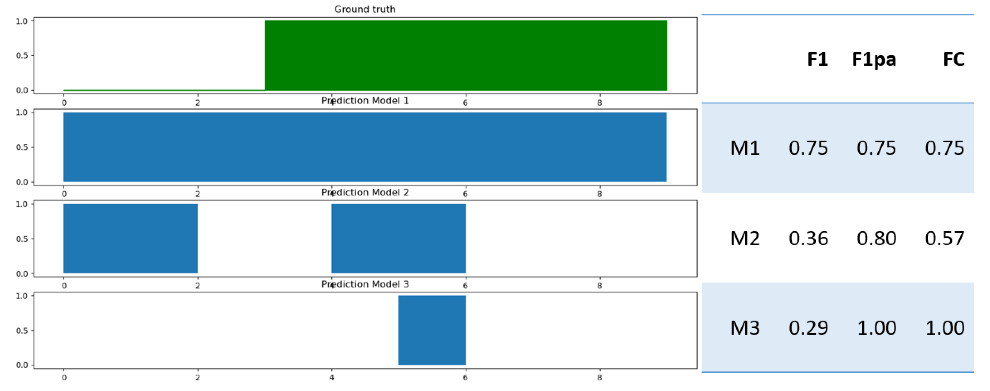
One can argue that the F1 score is not an optimal metric for anomaly detection, as it tends to produce low scores, even though the anomaly was detected [31]. This can be seen in Figure 3, where the F1 score for anomaly detection model 3 is only 0.29, although the anomaly was detected. For this reason, a new metric was introduced by Hundman et al. [3]: the F1 point adjust (F1pa). An in-depth definition and description can be found in [32]. The basic idea behind it is that if at least one moment in a contiguous anomaly segment is detected as an anomaly, the entire segment is then considered to be correctly predicted as an anomaly. This is referred to as event-based scoring. The F1 point adjust score is then calculated with the adjusted predictions.
However, the F1pa does not come without criticism. Kim et al. [32] pointed out that it overestimates the quality of anomaly detection models. Anomaly detection model 2 in Figure 3, for example, receives an F1pa score of 0.8 while predicting an anomaly where none occurred. In order to compensate for this behaviour, the composite F1 score (FC) was introduced by Garg et al. [33]. The FC score is calculated similarly to the F1 score by taking the harmonic mean of precision and recall. The recall uses event-based calculations instead of instance-based, whereas the precision uses instance-based calculations.
As is clear from our line of argument, no single metric is able to capture the quality of the diagnostic models to a full extent. No metric is flawless; suitable metrics should be chosen carefully. Of course, such a choice should be made application-specific and with the purpose of the anomaly detection model output in mind. Because we aim to provide an adaptive framework, which is not application-specific, we do not pick a single metric but instead optimise all three presented metrics: F1 score, F1pa score and FC score. This is explained in more detail in Section 3.2.

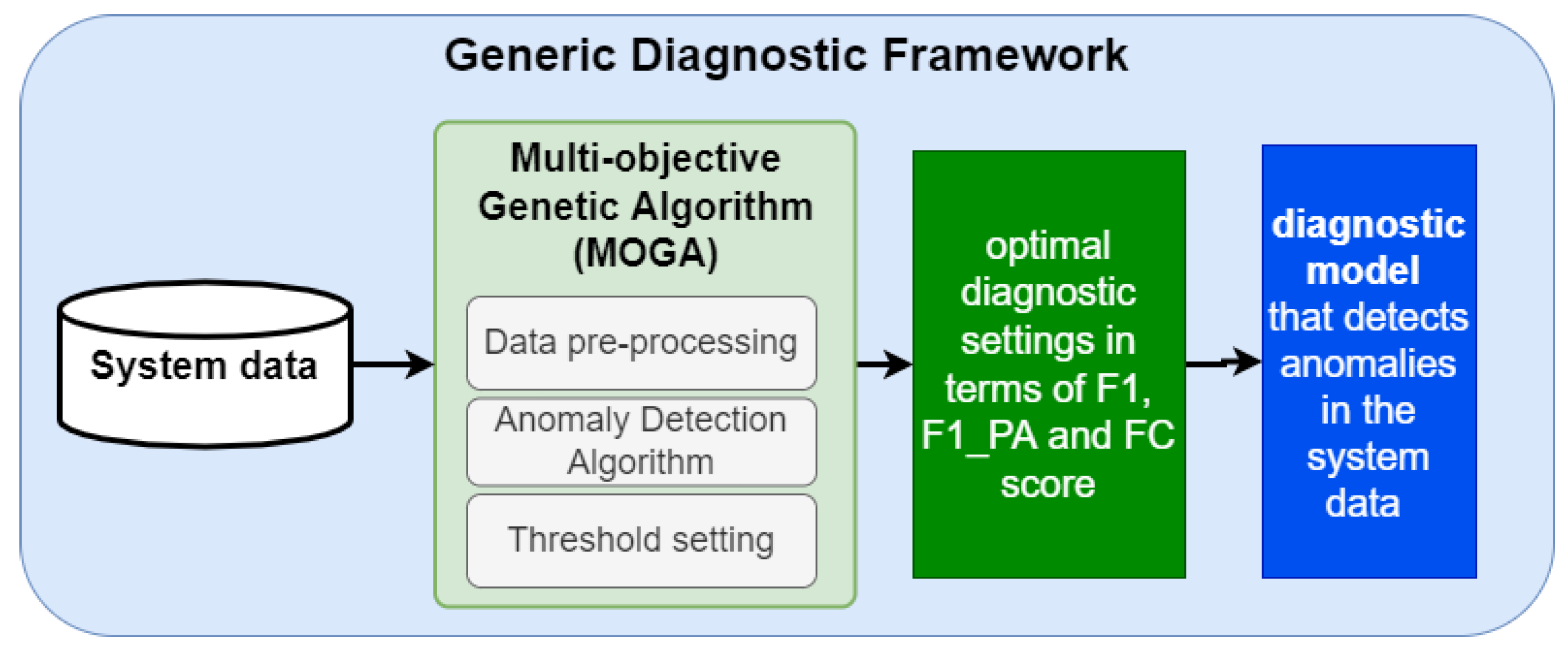
3.2. The Generic Diagnostic Framework

The GDF, visually represented in Figure 4, outputs for given system data and, in terms of pre-defined metrics, an ’optimal’ anomaly detection model for the system. We assume that the underlying system data is time series data and comes in the form of sensor readings/telemetry values, which are continuously recorded over a certain period of time. An example of what this data could look like can be found in Section 4.2 and Section 4.4. The GDF includes a range of data pre-processing techniques, anomaly detection, and thresholding techniques. The choice of the respective techniques is approached as a multi-objective optimisation problem, simultaneously allowing optimising all three selected metrics: F1 score, F1pa score and FC score. To be more precise, the problem of finding the respective combination of techniques can be formulated as the following optimisation problem: The objective function is to maximize the F1, F1pa and FC scores of the anomaly detection algorithm together with the data pre-processing and thresholding techniques on the system dataset. The output of such an optimisation is a Pareto front, which consists of multiple individuals outperforming the remaining individuals in terms of the chosen metrics. A detailed explanation of the workings and dynamics of the framework and the multi-objective optimisation problem can be found in [30], in which the Generic Prognostic Framework is presented, which is the basis for the GDF presented here. In the following, we go into more detail concerning the genetic algorithm which is used to solve the optimisation problem in Section 3.2.1, the data pre-processing in Section 3.2.2, the anomaly detection methods in Section 3.2.3 and the thresholding techniques in Section 3.2.4 included in the framework.

3.2.1. Multi-Objective Genetic Algorithm

Genetic algorithms are based on the concepts of natural selection and genetics [34]. Due to their flexibility, GAs are able to solve large optimisation problems. In addition, since GAs are a population-based approach, they are well-suited for multi-objective optimisation problems, like in our case, simultaneously optimising three different metrics (F1 score, F1pa and FC score) [35]. This is what makes them good candidates for our optimisation problem. A wealth of solutions are created, and their respective fitness values are computed in every generation [36]. We make use of the Non-dominated Sorting Genetic Algorithm II (NSGA-II, introduced in [37]). It ranks candidate solutions with the fast non-dominated sorting method and uses a crowding distance as a diversity mechanism. The algorithm is well-tested, has been used in many applications and is efficient.
A GA consists of several steps as presented in Algorithm 1. The process is as follows:
-
A population is initialised, composed of a set of individuals (i.e., solutions to the optimisation problem).
-
The best-fitted individuals are selected based on a fitness metric which represents the objective.
-
In the following step, the selected individuals undergo a cross-over and mutation process to produce new children for a new generation of individuals.
-
This process is repeated over a number of generations until the algorithm converges or a stopping criterion is achieved.
Algorithm 1: Genetic Algorithm
Aerospace 10 00673 i001
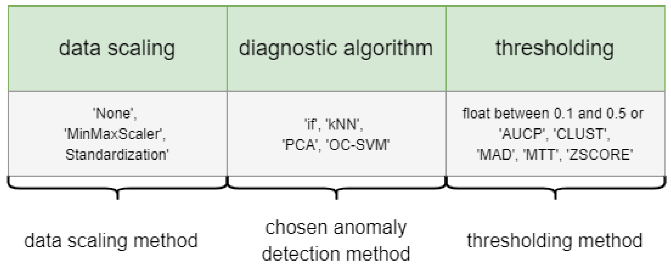
The Multi-objective GA (MOGA) takes as an input from the system data and outputs a set of Pareto optimal solutions. A solution combines a data re-balancing technique, an anomaly detection method and a thresholding technique. Therefore, an individual of the MOGA takes the form as shown in Figure 5.

3.2.2. Data Pre-Processing

Data pre-processing is an essential step in the application of data-driven diagnostic methodologies. Commonly used data pre-processing methods for time series data are data standardization or normalization and signal processing methods, such as time-domain analysis, frequency-domain analysis, time–frequency analysis and sliding windows to de-noise data [38]. Furthermore, machine learning algorithms are often combined with feature extraction or feature selection algorithms. Since the framework is supposed to be adaptive to different systems, data pre-processing heavily depends on the nature of the data and the underlying system. In addition, failure behaviour dynamics and the way system degradation is represented in the underlying data influence the selection of those methods. In order to make the framework as adaptive as possible, we only include the minimum amount of required data pre-processing techniques. However, data normalisation and standardisation are necessary steps when applying ML algorithms, especially when the input data is multi-dimensional, such as in our case. Therefore, the two included methods for the data scaling are ’Standardization’ and ’MinMaxScaler’, or normalisation. Standardization, or also Z-Score normalisation, results in variables with the properties of a standard normal distribution. Normalisation, or the MinMax scaler, scales the input data to a pre-defined range, in this case [ 0 , 1 ] . Note that the cost of having this bounded range—in contrast to standardization—is that we can end up with smaller standard deviations, which can suppress the effect of anomalies. We also include the option ’None’, in which no scaling method is chosen.

3.2.3. Anomaly Detection

The anomaly detection methodologies represented in the framework should capture as many different techniques with different underlying dynamics as possible. For this reason, we based the selection of the methods on the taxonomy of AI-based anomaly detection methods in Section 2. In Figure 1, we differed four categories of anomaly detection methods, namely proximity-based, ensemble-based, domain-based and reconstruction-based methodologies. In the framework, one representative method from each of the four categories is included. Those are:
  • k-Nearest Neighbours (KNN) as presented in [39], which measures the distance between data points and classifies the points with the highest distance from the other instances as anomalous.
  • Isolation Forests (iF) as introduced by [40], which build tree structures to isolate data points (which are considered as anomalies).
  • Principal Component Analysis (PCA), which performs a linear dimensionality reduction into a lower dimensional space to compute outlier scores.
  • One Class-Support Vector Machines (OC-SVM), which estimate the support of a high-dimensional distribution and thereby define non-linear boundaries around the region of the normal data (separating the remaining points as anomalies).
In order to define the initial settings for each of the four techniques, the hyperparameters are first tuned for each. Table 1 contains the respective parameters and tested values.
Note that all our experiments were conducted in Python, and for the anomaly detection methods, the PyOD toolbox is used [41].

3.2.4. Thresholding

As highlighted in Section 2, thresholding methods can help improve the quality of anomaly detection methods. In the PyOD toolbox, every anomaly detection method returns outlier scores but also has an integrated thresholding method to calculate the labels. We include both the default threshold setting provided by the PyOD algorithms and additional thresholding techniques in the framework. In a MOGA individual, see Figure 5, the default threshold methods are represented by the float options for the threshold settings (0.1 to 0.5). This is because PyOD calculates the thresholds based on the contamination rate, which is the rate of expected anomalies in a dataset. In the optimisation process of the MOGA, this can be regarded as an additional hyperparameter for the anomaly detection methods used being tuned. In order to provide a truly unsupervised and adaptive framework, several thresholding methods apart from the pre-implemented ones are included in the framework. These are
  • the Area Under Curve Percentage (AUCP);
  • the Clustering-based method (CLUST);
  • the Median Absolute Deviation (MAD);
  • the Modified Thompson Tau Test (MTT); and
  • the Z-Score (Z-Score).
The AUCP makes use of the area under the curve (AUC) to calculate the outlier labels using the outlier scores [16]. The AUC is defined as
A U C = l i m x i n f i = 1 n f ( x ) δ x ,
with f ( x ) denoting the curve, δ x the incremental step size of rectangles whose areas are summed up and n the number of points in the outlier scores. The curve is obtained by calculating the probability density function of the outlier scores (values between 0 and 1), calculated using a kernel density estimation. The incremental step size δ x is set to 1 2 n . Then the AUC is continuously calculated in steps from left to right from the data range starting from 0 and arriving at a number of AUCs, namely A U C 0 , , A U C k . To obtain the threshold, another variable, l i m , is introduced as follows:
l i m = x ¯ + | x ¯ x ˜ | ,
where x ¯ is the mean outlier score and x ˜ the median outlier score. The threshold is defined as:
t h r e s = A U C j , with j = m i n { k { 1 , , n } | A U C k > l i m · A U C } ,
with l i m as defined in Equation (4) and A U C as defined in Equation (3). In other words, the threshold is set to the first AUC greater than the total AUC of the pdf multiplied by the l i m .
The Clustering-based method used in this study creates clusters of the outlier scores using hierarchical clustering, classifying objects within clusters as “normal” and objects outside as “outliers” [42].
The MAD introduced in [17] is motivated by the fact that the median is more robust against outliers than the mean. The threshold in this case is calculated as follows:
T m i n = m e d i a n ( X ) a M A D
T m a x = m e d i a n ( X ) + a M A D ,
with M A D = 1.4826 m e d i a n ( | X m e d i a n ( X | ) , a a user variable, set to three in our case and X in the outlier scores.
The Modified Thompson Tau test (MTT) is a modified univariate t-test that eliminates outliers that are more than a number of standard deviations away from the mean [43]. The Tau critical value is defined as
τ = t · ( n 1 ) n n 2 + t 2 ,
with n denoting the number of outlier scores and t the Student t-value. The method works iteratively and recalculates the Tau critical value after each outlier removal until the dataset no longer has any data points that fall outside the criterion, which is set to three standard deviations in this case.
Finally using the Z-Score as a thresholding technique (see [20] for further details) is based on the assumption that the outlier scores, x, are normally distributed with a mean μ and variance σ 2 , i.e., x N ( μ , σ 2 ) . In this case the underlying Z-Score can be calculated as
Z = x μ σ .
The data are then labelled as “normal” if the following criterion holds:
| Z S c o r e | a ,
with a as an input variable, set to a = 3 in our case.
The above-mentioned methods are implemented using the PyThres library, a toolkit for thresholding outlier detection.

4. Case Studies and Results

The GDF presented in Section 3 is applied to three satellite and spacecraft system datasets: The first two, presented in Section 4.2 and Section 4.3 are publicly available and commonly used datasets in the literature, while the third, presented in Section 4.4, is a real-life satellite system dataset provided by the ESA. We try to understand whether the GDF provides a robust diagnostic assessment for all the datasets by comparing the results to baseline machine learning algorithms. A thorough assessment of the dynamics of the framework and the way the metrics influence choices is given by comparing the multi-objective optimisation framework to a single-objective approach. The single-objective optimisation problem can be formulated as follows: The objective function is to maximize the F1 score (the F1pa score) of the anomaly detection algorithm together with the data pre-processing and thresholding techniques on the system dataset. We argue (see Section 3) that including the thresholding methodologies makes the GDF more adaptive and provides significantly better results, which is shown by comparing the two versions of the GDF: one including the thresholding methods and one without them. First, in Section 4.1, we give an overview of the settings used within the GDF and how it was applied to the three datasets.

4.1. Application of the GDF to the Datasets

Several hyperparameters need to be set for the MOGA (see [30] for more details). In Algorithm 1, it can be seen that cross-overs from two other individuals create new individuals. The cross-over rate is the probability with which two individuals are crossed and is set to 0.5 . Furthermore, individuals can be mutated to evolve over time. The mutation rate is the probability of mutating an individual and is set to 0.1 . The algorithm is run either until it converges to an optimal solution or a stopping criterion is achieved, and we set the maximum number of generations to 20. The number of individuals in the population is set to 50.
Each of the datasets presented below consists of multiple subsets corresponding to components. The subsets are split into training and testing data, respectively. An anomaly detection model is trained on each of the training datasets and tested on each of the testing datasets, and the final score is computed using the mean of all the scores on each sub-dataset. The results are compared to the baseline models. The four baseline models are PCA, iF, KNN and OC-SVM trained on the dataset without applying any prior hyperparameter tuning. In other words, they are obtained using the four anomaly detection algorithms with the default settings as implemented in the Python PyOD package.

4.2. SMAP Dataset

The data from the NASA Soil Moisture Active Passive (SMAP) satellite forms a publicly available expert-labelled telemetry anomaly dataset [3]. It contains 54 multi-dimensional time-series sub-datasets. Each sub-dataset is split into a training and testing set. An example of the telemetry values can be seen in Figure 6.
First, the initial diagnostic algorithms are determined by performing hyperparameter tuning as presented in Section 3.2.3. This results in the initial anomaly detection models with their settings presented in Table 2.

4.2.1. Resulting Pareto Front Compared against the Baseline

The output of the GDF is a Pareto front consisting of multiple individuals with different settings for the data pre-processing, anomaly detection and thresholding techniques. Table 3 contains the Pareto front for the SMAP dataset.
Figure 7 shows the range of the three different scores (F1, F1pa and FC) for all individuals and the individuals in the Pareto front.
It can be seen in Table 3 that for this dataset, the choice of the anomaly detection method is KNN as it beats the other anomaly detection methods in all cases. Furthermore, the individuals in the Pareto front, in terms of all the metrics, are very close to each other. For example, the F1 scores range from 0.19 to 0.249 and the FC scores from 0.317 to 0.364. This can also be seen in Figure 7. One further notable thing is that it seems as if the threshold setting has the biggest influence on the scores. For example, the F1pa score when using normalization together with KNN and MAD is 0.588, while the F1pa score for the same settings but using the Z-Score is 0.676. We will go into more detail on this in Section 4.2.3.
Table 4 shows the results of the baseline models. For a better assessment, a comparison of the baseline models against the best performing individuals of the Pareto front in terms of the respective scores can be found in Table 5.
When looking closer at Table 4 and the results in terms of the F1 score, it becomes clear why the KNN was chosen. The performance of other algorithms is much worse, while the OC-SVM outperforms the other algorithms in terms of the F1pa score. Table 5 reveals that the thresholding improves the results in terms of the F1pa score, resulting in the performance of all the individuals of the Pareto front outperforming all the baseline models in terms of the F1pa score. For the FC score, the results are similar to the F1pa score, but here the KNN baseline model already outperforms the OC-SVM model.

4.2.2. Comparing Multi-Objective Optimisation with Single-Objective Optimisation

Performing single-objective optimisation and setting the metrics to both the F1 and F1pa scores results in the following individuals chosen by the GDF:
  • When optimising towards an F1 score, the best individual has the following settings: normalisation, KNN, and a Z-Score of 0.04, with an F1 score of 0.249.
  • When optimising towards the F1pa score, the best individual has the following settings: normalisation, KNN, and Z-Score, with an F1pa score of 0.676.
In this case, Figure 7 already shows that the resulting scores within the Pareto front do not cover a wide range (e.g., the lowest FC score is 0.317, which is quite close to 0.364, the top score). Following this observation, we expect the results of single-objective optimisation to be very close to those of the MOGA, which they are. In most cases, increasing F1pa causes the F1 score to decrease. So, all in all, while in this case, single-objective optimisation would form a formidable alternative to using the MOGA, optimising towards a single metric always means a compromise in terms of another metric. Therefore, the metric should be chosen with care.

4.2.3. The Effect of Including Thresholding Methods

Table 6 shows the results of using the GDF using just the default settings of the PyOD algorithms (which set the contamination rate to 0.1) for the label computation.
To make the effect of this clearer, Table 7 shows the best individual output by the GDF with default thresholding and when including the selected thresholding techniques.
While in terms of the F1 score, the thresholding techniques have little effect on the quality of the results (see Table 7), including more elaborate thresholding methods improves the scores by quite a bit in terms of the F1pa and FC scores.

4.3. MSL Dataset

Another publicly available spacecraft telemetry dataset that contains expert-labelled anomalous data is data from the Mars Science Laboratory (MSL) rover, Curiosity. Similarly, the SMAP dataset consists of 27 sub-datasets, each containing telemetry values from 25 sensors [44].
The hyperparameter tuning to give the initial diagnostic algorithms results in the settings listed in Table 8.

4.3.1. Resulting Pareto Front Compared against Baseline

The Pareto front for the MSL dataset is presented in Table 9.
Figure 8 shows the range of the three different scores (F1, F1pa and FC) for all individuals and Pareto front individuals.
The performance of the individuals in the Pareto front for the MSL data, as can be seen in Figure 8, covers a wider range than for those for the SMAP dataset. For example, the F1 ranges from 0.107 to 0.259 and the F1pa from 0.524 to 0.734. In addition, in this case, it is less clear which anomaly detection method is the best since three of the four anomaly detection techniques, IF, PCA and KNN, are represented in the Pareto front. Using KNN results in the highest scores in terms of F1 but the lowest in terms of F1pa. The iF models receive medium scores in terms of both F1 and F1pa but score lowest in terms of FC, while the PCA models score highest in terms of F1pa but lowest in F1.
Table 10 shows the results of the baseline models. A comparison of the baseline models against the best performing individuals of the Pareto front in terms of their respective scores can be found in Table 11.
Again, we see that in terms of the F1 score, there is no significant improvement, but the individuals in the Pareto front score much higher in terms of the F1pa and FC scores. The F1pa score, as can be seen in Table 11, improved from 0.559 (for the baseline model iF) to 0.734 (when using normalization, PCA and AUCP).

4.3.2. Comparing Multi-Objective Optimisation with Single-Objective Optimisation

Performing single-objective optimisation and setting the metrics to both the F1 and F1pa scores results in the following individuals chosen by the GDF:
  • When optimising towards an F1 score, the best individual has the following settings: normalisation, KNN, and MAD, with an F1 score of 0.259.
  • When optimising towards an F1pa score, the best individual has the following settings: normalisation, PCA, and AUCP, with an F1pa score of 0.734.
In the case of single-objective optimisation for the MSL dataset, it can be observed that the GA outputs normalisation, KNN and MAD when optimising the F1 score, which results in the lowest scoring individual contained in the Pareto front (see Table 9) in terms of the F1pa score. The same is true and vice versa: The best performing individual in terms of the F1pa score is the lowest scoring individual in terms of the F1 score. Therefore, it becomes visible here that optimising towards a single metric comes at the cost of a lowered score in terms of another metric.

4.3.3. The Effect of Including Thresholding Methods

Table 12 shows the results of using the GDF with the default settings of PyOD for the label computation.
Table 13 shows the best individuals output by the GDF with default thresholding and when including the selected thresholding techniques.
Similarly, as for the SMAP dataset, in Table 13 it can be seen that the biggest difference when including the elaborate thresholding methods is achieved in terms of the F1pa and FC scores. Compared to the results of the baseline models (see Table 11), the scores improve slightly when including data pre-processing techniques.

4.4. Satellite Reaction Wheel Dataset

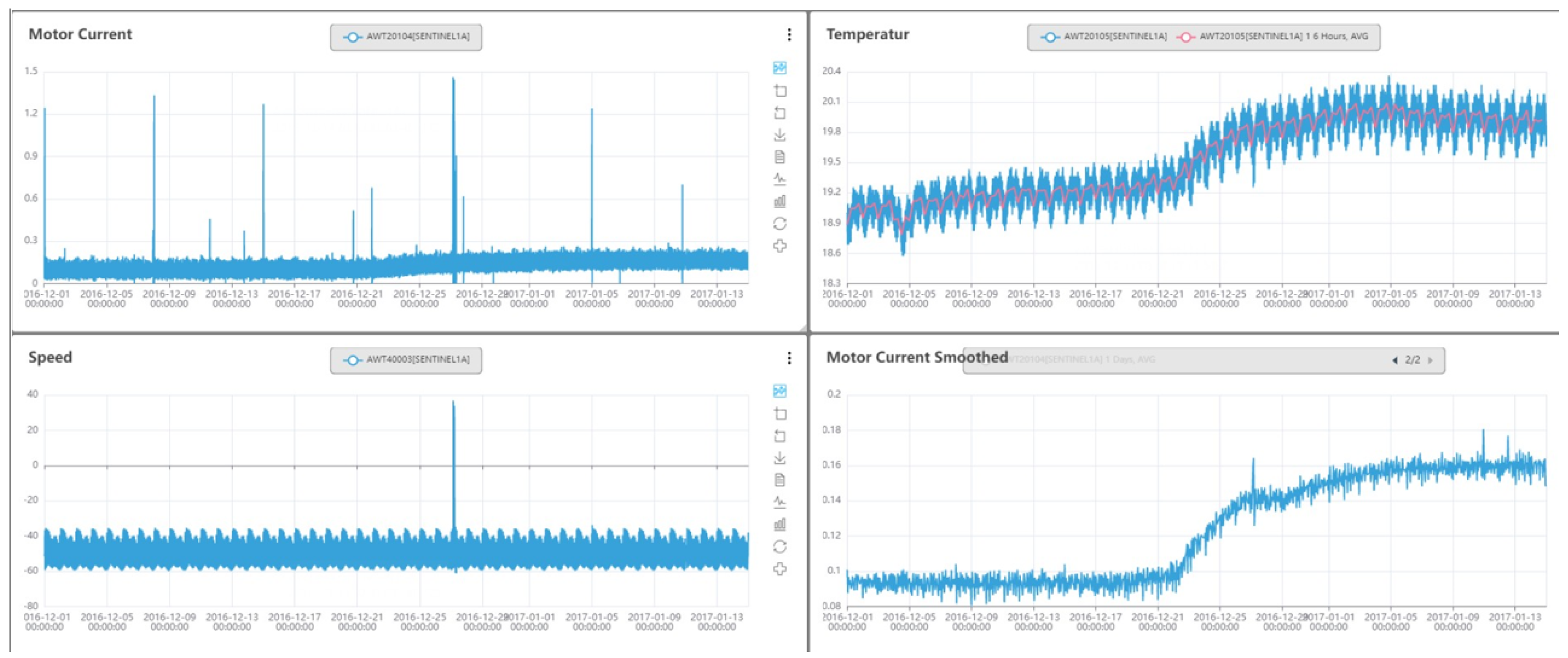
The third dataset used in this study contains telemetry data from reaction wheels (RWL) operated on the ESA Earth Observation satellites in a two-satellite constellation. Each of the two satellites carries four reaction wheels. A substantial amount of health-related RWL data has so far been collected during this mission, which can be utilised for anomaly detection. During the operation time, however, only six anomalies occurred, which, together with anomaly reports, were used to create the test dataset for this study. Each RWL is equipped with 10 sensors recording health-related telemetry values. An example of such telemetry sensor readings can be seen in Figure 9.
The hyperparameter tuning giving the initial diagnostic algorithms results in the settings listed in Table 14.

4.4.1. Resulting Pareto Front Compared against the Baseline

Table 15 contains the output of the GDF applied to the ESA dataset, i.e., the individuals in the Pareto front.
Figure 10 shows the range of the three different scores (F1, F1pa and FC) for all individuals and the individuals in the Pareto front.
Applying the GDF to the ESA dataset results in the largest Pareto front of the three datasets. This is not surprising that therefore the range of performance of the Pareto front individuals is quite high (see Figure 10), e.g., the F1 score ranges from very close to 0 to 0.623. It can also be seen that the highest performance in terms of the F1pa score results in a very poor F1 score: For example, the individual KNN MAD has an F1 score of 0.0314 and the individual using KNN with the ZSCORE an F1 score of 0.059, while both of these individuals have an F1pa score of 1.0. It can be said that, in general, increasing the F1pa score comes at the cost of lowering the F1 score (see Table 15). Similarly, increasing the FC score results in lower F1 scores. Furthermore, the thresholding techniques do not seem to have a particularly strong effect on the scores when using KNN for anomaly detection (see Table 15).
Table 16 shows the results of the baseline models. The comparison of the baseline models to the best performing individuals of the Pareto front in terms of their respective scores can be found in Table 17.
When comparing the Pareto front individuals to the baseline models, we again see that in terms of F1, there is not much improvement in the results. Still, significant improvement is visible in terms of the F1pa and FC scores.

4.4.2. Comparing Multi-Objective Optimisation with Single-Objective Optimisation

Performing single-objective optimisation and setting the metrics to both the F1 score and F1pa results in the following individuals chosen by the GDF:
  • When optimising towards an F1 score, the best individual has the following settings: normalisation, KNN, 0.14 with an F1 score of 0.621.
  • When optimising towards the F1pa score, the best individual has the following settings: normalisation, KNN MAD with an F1pa score of 1.0.
Here, the effect of including multiple metrics in the optimisation is visible because many individuals score high F1pa scores in the Pareto front. Therefore, considering the F1 score in addition to the F1pa gives a good insight into performance (see the previously pointed out very poor performing individuals in terms of F1 score). Again, the FC score is mostly in alignment with the F1pa score, i.e., increasing the F1pa score usually simultaneously increases the FC score.

4.4.3. The Effect of Including Thresholding Methods

Table 18 presents the results of using the GDF including default thresholding techniques.
Again, to give a clearer insight into the results, Table 19 shows the best individuals returned by the GDF with default thresholding and with the additional thresholding techniques.
Compared to Table 16, we see that using pre-processing data methods on the ESA dataset does not improve the results as much as for the MSL and SMAP datasets. Furthermore, we see that again, in terms of the F1pa and FC scores, including thresholding techniques result in much better anomaly detection models. In contrast, in terms of the F1 score, the effect is less significant.

4.5. Discussion

In this section, we present the findings of the results regarding the three main objectives as highlighted in Section 1 and at the beginning of Section 4 based on the results. The results show that the framework is adaptive to different datasets and outperforms the baseline algorithms in all three case studies (see Table 5, Table 11 and Table 17). Furthermore, the framework indicates as to which methods to focus further on and which methods perform well for a given dataset. For the SMAP dataset, the results presented in Section 4.2, a single anomaly detection method (KNN) can be singled out from the four input techniques. For the MSL dataset, presented in Section 4.3, this is not so clear, both iF and KNN could be considered. Similarly for the ESA dataset (see Section 4.4), the Pareto front is much bigger, which makes it harder to choose the ’best’ set of methods. This points out the importance of choosing suitable metrics for evaluating the models.
Including three different metrics in the framework makes it more robust, which is especially visible in the results on the ESA dataset (see Table 15). In this case the best results in terms of the F1pa score receive the lowest score in terms of the F1 score. In general, higher F1pa and FC scores result in lower F1 scores. Mostly the FC score is aligned with the F1pa score, but this is not always true. For example, for the MSL dataset in Table 9, we see that the highest scoring individual in terms of the F1pa score (normalisation PCA and AUCP) reaches an F1pa score of 0.734 and an FC score of 0.313. In contrast, the highest-scoring individual in terms of the FC score (KNN and ZSCORE) with an FC score of 0.346 has an F1pa score of only 0.553.
Finally, including thresholding techniques significantly improves the results. Throughout all three datasets, shown in Table 7, Table 13 and Table 19, both the F1pa and FC scores can be improved when using thresholding techniques. For example, in the ESA dataset (Table 19), the FC score is improved from 0.768 to 1.0 and the F1pa score from 0.876 to 1.0 when including thresholding techniques in the framework.

5. Conclusions

A GDF was presented with its capability to automatically chose optimal data pre-processing, anomaly detection and thresholding techniques simultaneously given system data. Overall, thresholding methods play an important role in anomaly detection and can significantly influence the quality of the resulting models. In addition, the optimisation metrics affect the choice of methods, and the optimisation towards a single metric is always a trade-off. Therefore, particular care should be taken when choosing suitable metrics to evaluate the anomaly detection models.
The next step in the development of the GDF could be to include more metrics in the model assessment or even perform a more thorough assessment towards applications. Another interesting direction for further research could be to look into systems operated under different operating conditions. Especially for satellite systems, for which failures or even anomalies are scarce, it would be an asset to be able to train models on systems in different satellite constellations, operated under similar conditions. Furthermore, the framework could be extended to include a wider range of techniques, e.g., by including more elaborate data pre-processing methods, deep learning anomaly detection methods or statistical algorithms.
All in all, the framework offers a quick way to assess the system data of complex systems towards their suitability for anomaly detection approaches. Based on the outputs, further decisions can be taken, and development and expertise can be streamlined in fruitful directions.

Author Contributions

Conceptualization, M.B., W.J.C.V., F.C. and B.F.S.; methodology, M.B., W.J.C.V. and B.F.S.; software, M.B.; validation, M.B.; writing—original draft preparation, M.B.; writing—review and editing, W.J.C.V., F.C. and B.F.S.; visualization, M.B.; supervision, W.J.C.V. and B.F.S.; funding acquisition, F.C. and B.F.S. All authors have read and agreed to the published version of the manuscript.

Funding

This research has received funding from the European Space Agency’s Co-sponsored PhD programme under contract number 4000131846/20/NL/MH/hm and by European Union’s Horizon 2020 program under the ReMAP project, grant No 769288.

Data Availability Statement

This research employed publicly available datasets for its experimental studies. The data in the case study are not publicly available due to the confidentiality requirement of the project.

Conflicts of Interest

The authors declare no conflict of interest.

References

  1. Chen, J.; Pi, D.; Wu, Z.; Zhao, X.; Pan, Y.; Zhang, Q. Imbalanced satellite telemetry data anomaly detection model based on Bayesian LSTM. Acta Astronaut. 2021, 180, 232–242. [Google Scholar] [CrossRef]
  2. Fuertes, S.; Picart, G.; Tourneret, J.Y.; Chaari, L.; Ferrari, A.; Richard, C. Improving spacecraft health monitoring with automatic anomaly detection techniques. In Proceedings of the 14th International Conference on Space Operations, Daejeon, Republic of Korea, 16–20 May 2016; pp. 1–16. [Google Scholar] [CrossRef] [Green Version]
  3. Hundman, K.; Constantinou, V.; Laporte, C.; Colwell, I.; Soderstrom, T. Detecting spacecraft anomalies using LSTMs and nonparametric dynamic thresholding. In Proceedings of the ACM SIGKDD International Conference on Knowledge Discovery and Data Mining, London, UK, 19–23 August 2018; pp. 387–395. [Google Scholar] [CrossRef] [Green Version]
  4. Zio, E. Prognostics and Health Management (PHM): Where are we and where do we (need to) go in theory and practice. Reliab. Eng. Syst. Saf. 2022, 218, 108119. [Google Scholar] [CrossRef]
  5. Basora, L.; Olive, X.; Dubot, T. Recent advances in anomaly detection methods applied to aviation. Aerospace 2019, 6, 117. [Google Scholar] [CrossRef] [Green Version]
  6. Zeng, Z.; Jin, G.; Xu, C.; Chen, S.; Zhang, L. Spacecraft Telemetry Anomaly Detection Based on Parametric Causality and Double-Criteria Drift Streaming Peaks over Threshold. Appl. Sci. 2022, 12, 1803. [Google Scholar] [CrossRef]
  7. Chen, Z.; Zhou, D.; Zio, E.; Xia, T.; Pan, E. Adaptive transfer learning for multimode process monitoring and unsupervised anomaly detection in steam turbines. Reliab. Eng. Syst. Saf. 2023, 234, 109162. [Google Scholar] [CrossRef]
  8. Shao, K.; He, Y.; Xing, Z.; Du, B. Detecting wind turbine anomalies using nonlinear dynamic parameters-assisted machine learning with normal samples. Reliab. Eng. Syst. Saf. 2023, 233, 109092. [Google Scholar] [CrossRef]
  9. Fink, O.; Wang, Q.; Svensén, M.; Dersin, P.; Lee, W.J.; Ducoffe, M. Potential, challenges and future directions for deep learning in prognostics and health management applications. Eng. Appl. Artif. Intell. 2020, 92, 103678. [Google Scholar] [CrossRef]
  10. Jardine, A.K.S.; Lin, D.; Banjevic, D. A review on machinery diagnostics and prognostics implementing condition-based maintenance. Mech. Syst. Signal Process. 2006, 20, 1483–1510. [Google Scholar] [CrossRef]
  11. Choi, K.; Yi, J.; Park, C.; Yoon, S. Deep learning for anomaly detection in time-series data: Review, analysis, and guidelines. IEEE Access 2021, 9, 120043–120065. [Google Scholar] [CrossRef]
  12. Nassif, A.B.; Talib, M.A.; Nasir, Q.; Dakalbab, F.M. Machine Learning for Anomaly Detection: A Systematic Review. IEEE Access 2021, 9, 78658–78700. [Google Scholar] [CrossRef]
  13. Chandola, V.; Banerjee, A.; Kumar, V. Anomaly Detection: A Survey. ACM J. 2009, 41, 1–58. [Google Scholar] [CrossRef]
  14. Khan, S.; Tsutsumi, S.; Yairi, T.; Nakasuka, S. Robustness of AI-based prognostic and systems health management. Annu. Rev. Control 2021, 51, 130–152. [Google Scholar] [CrossRef]
  15. Basora, L.; Bry, P.; Olive, X.; Freeman, F. Aircraft Fleet Health Monitoring using Anomaly Detection Techniques. Aerospace 2021, 8, 103. [Google Scholar] [CrossRef]
  16. Ren, K.; Yang, H.; Zhao, Y.; Chen, W.; Xue, M.; Miao, H.; Huang, S.; Liu, J. A Robust auc maximization framework with simultaneous outlier detection and feature selection for positive-unlabeled classification. IEEE Trans. Neural Netw. Learn. Syst. 2019, 30, 3072–3083. [Google Scholar] [CrossRef] [PubMed] [Green Version]
  17. Archana, N.; Pawar, S.S. Periodicity Detection of Outlier Sequences Using Constraint Based Pattern Tree with MAD. arXiv 2015, arXiv:1507.01685. [Google Scholar]
  18. Rengasamy, D.; Rothwell, B.C.; Figueredo, G.P. Towards a more reliable interpretation of machine learning outputs for safety-critical systems using feature importance fusion. Appl. Sci. 2021, 11, 1854. [Google Scholar] [CrossRef]
  19. Xiao, Z.; Yan, Q.; Amit, Y. Likelihood regret: An out-of-distribution detection score for variational auto-encoder. Adv. Neural Inf. Process. Syst. 2020, 33, 20685–20696. [Google Scholar]
  20. Bagdonavičius, V.; Petkevičius, L. Multiple outlier detection tests for parametric models. Mathematics 2020, 8, 2156. [Google Scholar] [CrossRef]
  21. Klawonn, F.; Rehm, F. Cluster Analysis for Outlier Detection. In Encyclopedia of Data Warehousing and Mining, 2nd ed.; IGI Global: Hershey, PA, USA, 2011; pp. 2006–2008. [Google Scholar] [CrossRef]
  22. Zhao, C.; Shen, W. Adaptive open set domain generalization network: Learning to diagnose unknown faults under unknown working conditions. Reliab. Eng. Syst. Saf. 2022, 226, 108672. [Google Scholar] [CrossRef]
  23. Alam, M.R.; Gerostathopoulos, I.; Prehofer, C.; Attanasi, A.; Bures, T. A framework for tunable anomaly detection. In Proceedings of the 2019 IEEE International Conference on Software Architecture, ICSA 2019, Hamburg, Germany, 25–29 March 2019; pp. 201–210. [Google Scholar] [CrossRef]
  24. Calikus, E.; Nowaczyk, S.; Sant’Anna, A.; Dikmen, O. No free lunch but a cheaper supper: A general framework for streaming anomaly detection. Expert Syst. Appl. 2020, 155, 113453. [Google Scholar] [CrossRef] [Green Version]
  25. Akiba, T.; Sano, S.; Yanase, T.; Ohta, T.; Koyama, M. Optuna: A Next-generation Hyperparameter Optimization Framework. In Proceedings of the 25th ACM SIGKDD International Conference on Knowledge Discovery & Data Mining, Anchorage, AK, USA, 4–8 August 2019. [Google Scholar]
  26. O’meara, C.; Schlag, L.; Faltenbacher, L.; Wicklerz, M. ATHMoS: Automated telemetry health monitoring system at GSOC using outlier detection and supervised machine learning. In Proceedings of the SpaceOps 2016 Conference, Daejeon, Republic of Korea, 16–20 May 2016; pp. 1–17. [Google Scholar] [CrossRef] [Green Version]
  27. O’meara, C.; Schlag, L.; Wickler, M. Applications of deep learning neural networks to satellite telemetry monitoring. In Proceedings of the 15th International Conference on Space Operations, Marseille, France, 28 May–1 June 2018; pp. 1–16. [Google Scholar] [CrossRef] [Green Version]
  28. Sun, W.; Paiva, A.R.C.; Xu, P.; Sundaram, A.; Braatz, R.D. Fault Detection and Identification using Bayesian Recurrent Neural Networks. Comput. Chem. Eng. 2019, 141, 106991. [Google Scholar] [CrossRef]
  29. Freeman, C.; Merriman, J.; Beaver, I.; Mueen, A. Experimental Comparison and Survey of Twelve Time Series Anomaly Detection Algorithms (Extended Abstract). In Proceedings of the IJCAI International Joint Conference on Artificial Intelligence, Vienna, Austria, 23–29 July 2022; Volume 72, pp. 5737–5741. [Google Scholar] [CrossRef]
  30. Bieber, M.; Verhagen, W.J. A Generic Framework for Prognostics of Complex Systems. Aerospace 2022, 9, 839. [Google Scholar] [CrossRef]
  31. Kim, G.Y.; Lim, S.M.; Euom, I.C. A Study on Performance Metrics for Anomaly Detection Based on Industrial Control System Operation Data. Electronics 2022, 11, 1213. [Google Scholar] [CrossRef]
  32. Kim, S.; Choi, K.; Choi, H.S.; Lee, B.; Yoon, S. Towards a Rigorous Evaluation of Time-Series Anomaly Detection. In Proceedings of the AAAI Conference on Artificial Intelligence, Online, 22 February– 1 March 2022; Volume 36, pp. 7194–7201. [Google Scholar] [CrossRef]
  33. Garg, A.; Zhang, W.; Samaran, J.; Savitha, R.; Foo, C.S. An evaluation of anomaly detection and diagnosis in multivariate time series. IEEE Trans. Neural Netw. Learn. Syst. 2021, 33, 2508–2517. [Google Scholar] [CrossRef] [PubMed]
  34. Holland, J.H. Adaptation in Natural and Artificial Systems; MIT Press: Cambridge, MA, USA, 1992. [Google Scholar] [CrossRef]
  35. Stanovov, V.; Brester, C.; Kolehmainen, M.; Semenkina, O. Why don’t you use Evolutionary Algorithms in Big Data? IOP Conf. Ser. Mater. Sci. Eng. 2017, 173, 012020. [Google Scholar] [CrossRef]
  36. Konak, A.; Coit, D.W.; Smith, A.E. Multi-objective optimization using genetic algorithms: A tutorial. Reliab. Eng. Syst. Saf. 2006, 91, 992–1007. [Google Scholar] [CrossRef]
  37. Deb, K.; Pratap, A.; Agarwal, S.; Meyarivan, T. A fast and elitist multiobjective genetic algorithm: NSGA-II. IEEE Trans. Evol. Comput. 2002, 6, 182–197. [Google Scholar] [CrossRef] [Green Version]
  38. Liu, R.; Yang, B.; Zio, E.; Chen, X. Artificial intelligence for fault diagnosis of rotating machinery: A review. Mech. Syst. Signal Process. 2018, 108, 33–47. [Google Scholar] [CrossRef]
  39. Angiulli, F.; Pizzuti, C. Fast outlier detection in high dimensional spaces. In Proceedings of the Principles of Data Mining and Knowledge Discovery: 6th European Conference, PKDD 2002, Helsinki, Finland, 19–23 August 2002; Volume 2431, pp. 15–27. [Google Scholar] [CrossRef] [Green Version]
  40. Liu, F.T.; Ting, K.M.; Zhou, Z.H. Isolation Forest. In Proceedings of the Eighth IEEE International Conference on Data Mining, Pisa, Italy, 15–19 December 2008; pp. 413–422. [Google Scholar]
  41. Zhao, Y.; Nasrullah, Z.; Li, Z. PyOD: A python toolbox for scalable outlier detection. J. Mach. Learn. Res. 2019, 20, 1–7. [Google Scholar]
  42. Lara, J.A.; Lizcano, D.; Rampérez, V.; Soriano, J. A method for outlier detection based on cluster analysis and visual expert criteria. Expert Syst. 2020, 37, e12473. [Google Scholar] [CrossRef]
  43. Sonneveld, B. Using the Mollifier Method to Characterize Datasets and Models: The Case of the Universal Soil Loss Equation; Technical Report; ITC: Kaunas, Lithuania, 1997. [Google Scholar]
  44. Challu, C.; Jiang, P.; Wu, Y.N.; Callot, L. Deep Generative model with Hierarchical Latent Factors for Time Series Anomaly Detection. In Proceedings of the 25th International Conference on Artificial Intelligence and Statistics, Virtual, 28–30 March 2022; Volume 151. [Google Scholar]
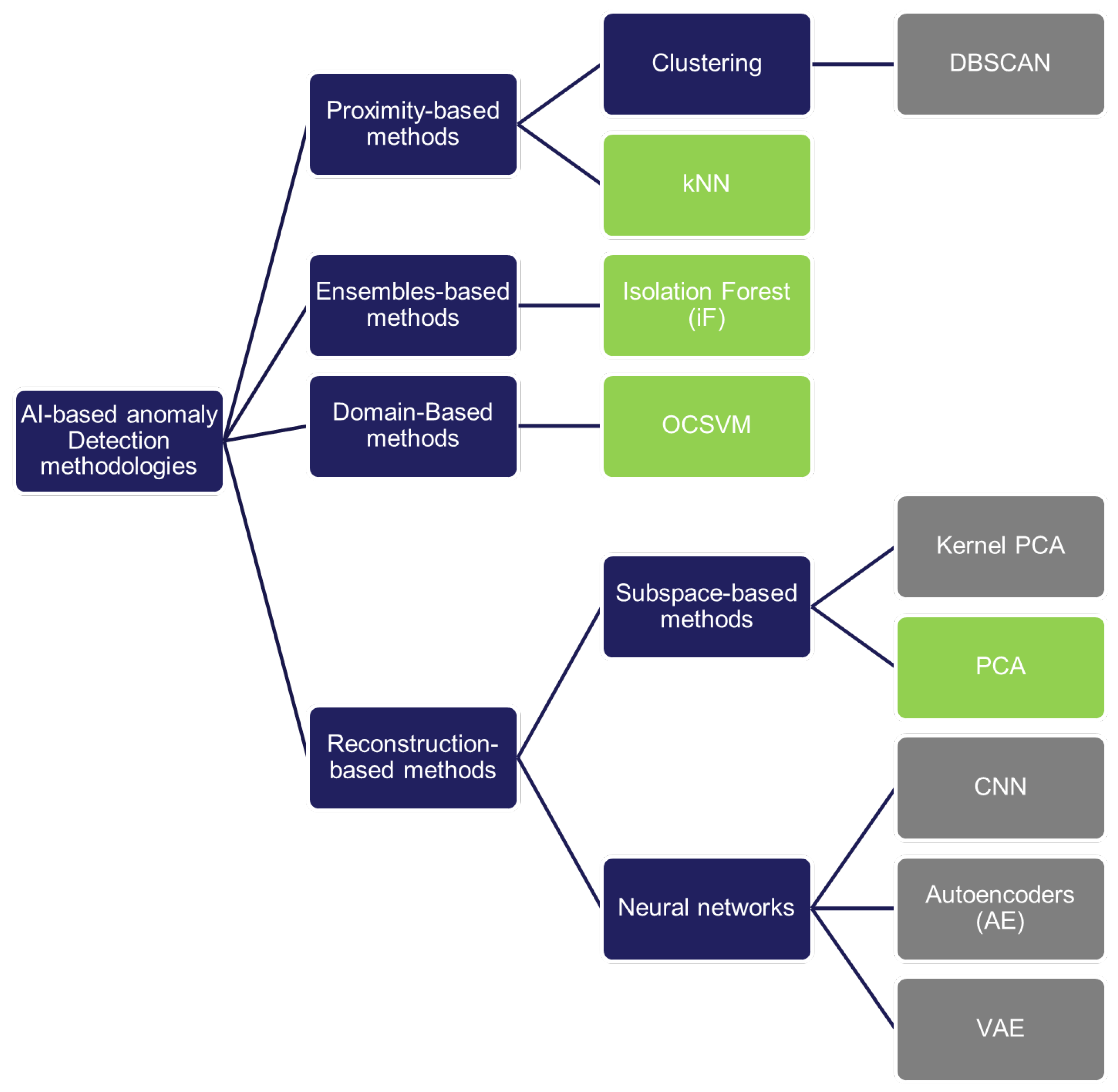
Figure 1. Taxonomy of AI-based anomaly detection methodologies. The methods marked in green are the ones included in the Generic Diagnostic Framework.
Aerospace 10 00673 g001
Figure 2. Confusion matrix.
Aerospace 10 00673 g002
Figure 3. Examples of anomaly detection model outputs and their resulting F1, F1pa and FC scores.
Aerospace 10 00673 g003
Figure 4. Elements of the Generic Diagnostic Framework.
Aerospace 10 00673 g004
Figure 5. GDF individual.
Aerospace 10 00673 g005
Figure 6. Example telemetry values from the sub-dataset A-1 in the SMAP dataset.
Aerospace 10 00673 g006
Figure 7. Scores of all individuals and Pareto front individuals for the SMAP dataset.
Aerospace 10 00673 g007
Figure 8. Scores of all individuals and Pareto front individuals for the MSL dataset.
Aerospace 10 00673 g008
Figure 9. Example telemetry values for the ESA dataset.
Aerospace 10 00673 g009
Figure 10. Scores of all individuals and Pareto front individuals for the ESA dataset.
Aerospace 10 00673 g010
Table 1. The hyperparameters and tested values for the four anomaly detection methods.
MethodHyperparameterDescriptionTested Values
Isolation Forestmax_samplesSize of the tree, number of samples to draw from X to train each base estimator100, 300, 500, 700
n_estimatorsNumber of trees in the ensemble (default is 100 trees)100, 200, 300, 400, 500
max_featuresNumber of features to draw from X to train each base estimator (default value is 1.0)5, 10, 15
KNNn_neighborsNumber of neighbours to use for k neighbours queries1, 4, 8, 12, 16
pParameter for Minkowski metric1, 2, 3
method
  • ‘argest’: use the distance to the kth neighbour as the outlier score
  • ‘mean’: use the average of all k neighbours as the outlier score
  • ‘median’: use the median of the distance to the k neighbours as the outlier score
‘largest’, ‘mean’, ‘median’
algorithmAlgorithm used to compute the nearest neighbours:
  • ‘ball_tree’ will use BallTree
  • ‘kd_tree’ will use KDTree
  • ‘auto’ will attempt to decide the most appropriate algorithm based on the values that passed the fit method
‘auto’, ‘ball_tree’, ‘kd_tree’
PCAn_components:Number of components to keepNp.arrange(1,20,2)
OC-SVMkernelSpecifies the kernel type to be used in the algorithm used to pre-compute the kernel matrix.‘rbf’, ‘poly’, ‘sigmoid’, ‘linear’
nuUpper bound on the fraction of training errors and a lower bound of the fraction of support vectors0.1, 1, 10, 100, 1000
gammaKernel coefficient for ‘rbf’, ‘poly’ and ‘sigmoid’.np.arange(0,1,0.2)
Table 2. Hyperparameter settings of the initial anomaly detection methods for the SMAP dataset.
AlgorithmHyperparameterChosen Value
PCAn_components5
iFn_estimators100
max_samples100
max_features10
KNNn_neighbors13
p1
method‘median’
algorithm‘auto’
OC-SVMnu0.1
Gamma0.6
kernel‘sigmoid’
Table 3. Pareto front individuals and scores for the SMAP dataset.
SettingsF1F1paFC
Normalization KNN MAD0.2130.5880.319
Normalization KNN 0.040.2490.5820.34
Normalization KNN ZSCORE0.190.6760.364
Standardization KNN MAD0.210.5980.317
Standardization KNN 0.040.2490.5820.34
Table 4. Baseline models and scores for the SMAP dataset.
AlgorithmF1F1_paFC
OC-SVM0.1830.5650.276
KNN0.2390.4270.301
iF0.0950.4570.175
PCA0.00.00.0
Table 5. Comparison of the baseline models to the respective best performing Pareto front individuals for the SMAP dataset.
BaselineGDF
SettingsKNNKNN 0.04
F10.2390.249
SettingsOC-SVMNormalization KNN ZSCORE
F1pa0.5650.676
SettingsOC-SVMNormalization KNN ZSCORE
FC0.2760.364
Table 6. Pareto front when default thresholding techniques are included for the SMAP dataset.
SettingsF1F1paFC
Normalization PCA0.1360.490.221
Normalization KNN0.2420.4270.302
Standardization KNN0.2420.4270.302
Standardization OC-SVM0.1030.5220.206
Table 7. Comparison of the best individuals when using default thresholding vs. using selected thresholding for the SMAP dataset.
GDF No ThresholdingGDF Incl Thresholding
SettingsStandardization/normalization KNNKNN 0.04
F10.2420.249
SettingsStandardization OC-SVMNormalization KNN ZSCORE
F1pa0.5220.676
SettingsStandardization/normalization KNNNormalization KNN ZSCORE
FC0.3020.364
Table 8. Hyperparameter settings of initial anomaly detection methods for MSL dataset.
AlgoHyperparamChosen Value
PCAn_components1
iFn_estimators500
max_samples100
max_features5
KNNn_neighbors13
p1
method‘largest’
algorithm‘auto’
OC-SVMnu0.1
Gamma0
kernel‘linear’
Table 9. Pareto front individuals and scores for the MSL dataset.
SettingsF1F1paFC
normalization PCA AUCP0.1070.7340.313
Normalization iF AUCP0.1840.6260.306
Normalization iF MAD0.1840.6260.306
Normalization iF 0.080.1840.6260.306
Normalization KNN CLUST0.2330.6200.36
Normalization KNN ZSCORE0.2490.5530.346
Normalization KNN MAD0.2590.5240.338
Table 10. Baseline models and scores for the MSL dataset.
AlgorithmF1F1_paFC
OC-SVM0.2080.530.324
KNN0.2510.4880.324
iF0.1440.5590.238
PCA0.1660.5540.261
Table 11. Comparison of the baseline models against the respective best performing Pareto front individuals for the MSL dataset.
BaselineGDF
SettingsKNNNormalization KNN MAD
F10.2510.259
SettingsiFNormalization PCA AUCP
F1pa0.5590.734
SettingsOC-SVM and KNNNormalization KNN CLUST/MAD/ZSCORE
FC0.3240.36
Table 12. Pareto front when default thresholding techniques are included for the MSL dataset.
SettingsF1F1paFC
Normalization iF0.1840740.5966670.282963
Normalization KNN0.2551850.5033330.325185
Standardization iF0.1814810.5874070.291852
Table 13. Comparison of the best individuals when using default thresholding vs. using selected thresholding for the MSL dataset.
GDF No ThresholdingGDF Incl Thresholding
SettingsNormalization KNNNormalization KNN MAD
F10.2550.259
SettingsNormalization iFNormalization PCA AUCP
F1pa0.5970.734
SettingsNormalization KNNNormalization KNN CLUST/MAD/ZSCORE
FC0.3250.36
Table 14. Hyperparameter settings for the initial anomaly detection methods for the the ESA dataset.
AlgorithmHyperparameterChosen Value
PCAn_components1
iFn_estimators100
max_samples400
max_features10
KNNn_neighbors5
p1
method‘mean’
algorithm‘auto’
OC-SVMnu0.1
Gamma0.8
kernel‘rbf’
Table 15. Pareto front individuals and scores for the ESA dataset.
SettingsF1F1paFC
Normalization PCA 0.020.4590.9710.841
Normalization PCA 0.040.4890.9490.8
Normalization PCA ZSCORE0.1130.9830.903
Normalization iF 0.020.4760.9390.817
Normalization KNN MAD0.0311.01.0
Normalization KNN ZSCORE0.0790.9830.921
Normalization KNN 0.060.6070.8390.794
Normalization KNN 0.080.6160.8270.78
Normalization KNN 0.140.6210.7910.741
Standardization PCA 0.040.4890.9490.8
Standardization PCA ZSCORE0.1130.9830.903
Standardization KNN 0.060.6070.8370.79
Standardization KNN 0.080.6170.8260.776
Standardization KNN 0.120.6190.8040.754
Standardization KNN 0.180.6230.770.724
Standardization KNN ZSCORE0.0591.00.994
Standardization OC-SVM MAD0.5310.9330.897
Standardization OC-SVM CLUST0.6010.9070.841
Table 16. Baseline models and scores for the ESA dataset.
AlgorithmF1F1_paFC
OC-SVM0.540.8490.736
KNN0.6130.8140.766
iF0.5390.8410.737
PCA0.3360.5970.499
Table 17. Comparison of the baseline models against the respective best performing Pareto front individuals for the ESA dataset.
BaselineGDF
SettingsKNNStandardization KNN 0.18
F10.6130.623
SettingsOC-SVMKNN MAD/ZSCORE
F1pa0.8491.0
SettingsKNNKNN MAD
FC0.7661.0
Table 18. Pareto front when default thresholding techniques are included for the ESA dataset.
SettingsF1F1paFC
Normalization PCA0.5360.8790.744
Normalization iF0.5470.8390.747
Normalization KNN0.6170.8160.769
Normalization OC-SVM0.540.8410.74
Standardization PCA0.5360.8790.744
Standardization iF0.5470.8390.747
Table 19. Comparison of the best individuals when using default thresholding vs. using selected thresholding for the ESA dataset.
GDF No ThresholdingGDF Incl Thresholding
SettingsNormalization KNNStandardization KNN 0.18
F10.6170.623
SettingsPCAKNN MAD/ZSCORE
F1pa0.8791.0
SettingsNormalization KNNKNN MAD
FC0.7681.0
Disclaimer/Publisher’s Note: The statements, opinions and data contained in all publications are solely those of the individual author(s) and contributor(s) and not of MDPI and/or the editor(s). MDPI and/or the editor(s) disclaim responsibility for any injury to people or property resulting from any ideas, methods, instructions or products referred to in the content.