Trajectory Optimization for Multi-Sensor Multi-Target Search and Tracking with Bearing-Only Measurements

Abstract

This paper proposes a trajectory optimization approach for multi-sensor multi-target search and tracking using bearing-only sensors. Based on the framework of the joint integrated probabilistic data association (JIPDA) filter, the intensity of potential unknown targets is updated according to the trajectories of the UAVs. The performance indices for target search and tracking are constructed based on, respectively, the intensity of unknown targets in the search area and the tracking error covariance. A dimensionless criterion, evaluating the search and tracking performance, is formulated and leveraged as the objective function of the UAV trajectory optimization problem. Simulations were carried out in different search and tracking scenarios to demonstrate the effectiveness of the proposed approach.

1. Introduction

Unmanned aerial vehicles (UAVs) have shown great potential in both civilian and military applications, such as surveillance [1], search and rescue [2], reconnaissance [3] and traffic management [4]. A key enabler of these applications is target tracking, i.e., extracting the target information from the sensor measurements. As target tracking is an information gathering process, it can greatly benefit from multi-UAV systems, in terms of accuracy, effectiveness and also reliability [5]. However, UAV swarms are typically equipped with passive onboard sensors—e.g., optical and infrared cameras—due to their low cost and energy efficiency. These image sensors can only provide bearing information on the targets, and their fields of view (FOVs) are extremely limited, which makes it difficult to employ them in multi-target tracking scenarios. In multi-target tracking, the number of targets is usually both unknown and time-varying [6,7]: thus, the UAVs are required to search the entire area for undiscovered targets. On the other hand, as the image sensors cannot provide relative range information, target tracking using these sensors often suffers from observability problems [8,9,10]. Therefore, trajectory optimization is required for the UAVs, to improve the overall tracking performance in multi-sensor multi-target tracking applications.

Trajectory optimization for jointly searching for undiscovered targets and for maintaining the tracking accuracy of discovered targets is a challenging problem, as search and tracking are competitive goals and sensor resources are limited. In recent years, the problem of multi-target search and tracking based on sensor trajectory optimization has attracted the interest of researchers. The authors in [11] estimated the appearing probability of undetected targets, using the occupation grid filter. Based on the assumption that the data association between the measurements and target is known a priori, they predicted the mutual entropy between the future measurements and the grid occupation probability and also the target states. They took the weighted sum of these as the objective function, and they constructed the planning problem for multi-target search and tracking with range sensors. In [12], a Voronoi-based control method was combined with the distributed form of the probability hypothesis density (PHD) filter, to develop a distributed sensor management method of searching and tracking for an unknown number of targets. By utilizing the Poisson multi-Bernoulli mixture (PMBM) filter, the intensity of undetected targets was modeled and iterated according to the UAV trajectories, and a single-sensor management approach was proposed, based on the Monte Carlo Tree Search (MCTS) method in [13]. The algorithm was verified under the conditions of both static and mobile sensors. To avoid the problem of high computational complexity caused by the increase of the number of Gaussian components, the authors replaced the Gaussian-mixture target birth model in [13] with uniform distribution at the edge of the monitoring region, and they approximated the predicted target intensity using the Rao-Blackwellized point mass filter (RB-PMF) in [14]. In [15], mutual entropy in information theory was used to define the value function of target tracking, and the search area was divided into grids. The probability of unknown targets in each grid was modeled as a Bernoulli variable, and the change of Shannon entropy before and after the update process was leveraged as the value function of the searching objective. According to the global criterion method (GCM), a multi-objective optimization objective function was constructed, and the planning problem for multi-target search and tracking was solved by enumeration. However, the above works assumed that the target positions could be directly obtained from the sensors or that the range between the UAV and the target was accessible.

In this paper, a new trajectory optimization method for multi-sensor multi-target search and tracking with passive onboard sensors is proposed. The contributions of this paper are twofold. The original JIPDA filter is modified to facilitate the multi-target search objective. To the best of the authors’ knowledge, the multi-target search and tracking problem has rarely been studied utilizing the JPDA-based filter. On the other hand, the dimensionless objective functions for search and tracking, respectively, are derived, and their weighted sum is used as the overall objective function, which makes it convenient to adjust the weights of the two goals.

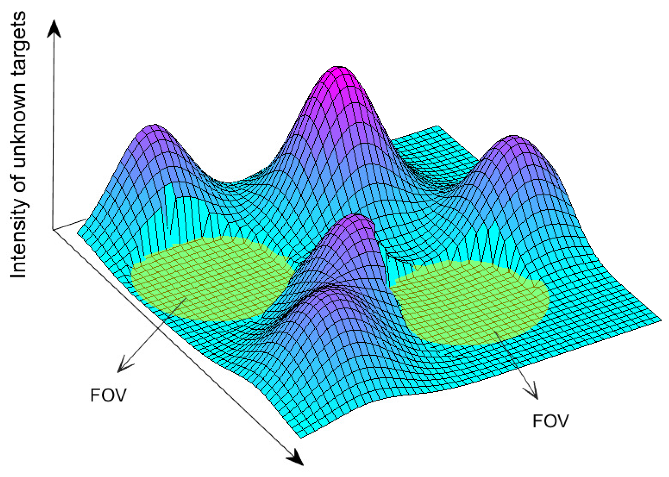
On the basis of the JIPDA filter, the intensity of unknown targets is considered and modeled, in the calculation of association probability. This is utilized as a metric to guide the UAV towards areas with a high probability of potential targets, to achieve the target searching goal. To facilitate the combination between the objective functions of searching and tracking, dimensionless metrics for these two objectives, respectively, are formulated, and their weighted sum is leveraged as the objective function for trajectory optimization. Typical scenarios were simulated, to evaluate the proposed approach, and the results reveal that the proposed method can well balance the search and tracking objectives and maintain acceptable multi-target tracking accuracy.

The rest of this paper is organized as follows. In Section 2, some system models are introduced, and the multi-sensor multi-target search and tracking problem is formulated. Section 3 provides the necessary preliminaries of the multi-target tracking filter and track-to-track fusion methods. The objective functions of multi-target search and tracking are derived first, and the multi-UAV trajectory optimization problem is then constructed in Section 4. The simulation results are presented in Section 5, and our conclusions are offered in Section 6.

2. Problem Formulation

This section describes some necessary system models, to facilitate the analysis in the following sections. Then, the problem of multi-sensor multi-target search and tracking is formulated.

2.1. System Models

In multi-target tracking, the target states at a certain timestamp can be modeled as a random finite set (RFS). Let $X_k=\left\{x_k^1,x_k^2,\dots x_k^{N_k}\right\}$ represent the set of multi-target states at time k, where $N_k$ denotes the number of targets at k, and where $x_k^i$ denotes the state vector of the ith target at time k. The state vector is four-dimensional, containing the position and speed of the target, and the state space model of the ith target is

$$x_k^i=f_{k-1}^i\left(x_{k-1}^i\right)+w_{k-1}^i,$$

(1)

where $f_k^i$ represents the state transition function and where $w_k^i$ is a Gaussian white noise with covariance matrix $Q_k^i$.

Suppose the number of measurements received by one UAV at time k is $M_k$, and the sensor measurement set is denoted as $Z_k=\{z_{0,k},z_{1,k},\dots z_{M_k,k}\}$, where $z_{j,k}(j\ne 0)$ represents the jth measurement, and where $z_{0,k}$ corresponds to the dummy measurement standing for miss detection and clutters. If the jth measurement of the sensor is originated from the ith target, the bearing-only measurement equation can be expressed as

$$z_{j,k}^i=h_k^i\left(x_k^i\right)+v_k=arctan\frac{y_{T,k}^i-y_{U,k}}{x_{T,k}^i-x_{U,k}}+v_k,$$

(2)

where $\left[x_{T,k}^i,y_{T,k}^i\right]$ and $\left[x_{U,k},y_{U,k}\right]$ are the positions of the ith target and the UAV, respectively, at time k, and where $v_k$ is a zero-mean Gaussian noise in angle measurements, with its covariance matrix being $R_k$.

As the number of targets is usually unknown in multi-target search and tracking scenarios, the track existence probability is also required to be estimated along with the target motion states. Let ${\chi }_k^i$ refer to the event of the ith track existing at scan k; the corresponding existence probability, i.e., $p({\chi }_k^i\mid Z_k)$, is denoted as $r_k^i$, for brevity. The existence probability is propagated using the Markov switching model as

$$r_{k|k-1}^i=P_S{r}_{k-1|k-1}^i,$$

(3)

where $P_S$ is the target surviving probability.

The probability of existence can be used as a measure for track management. A target becomes confirmed when its existence probability reaches to a predefined track confirmation threshold $r_c$, and it will be removed from the target set when $r_k^i$ falls below a termination bound $r_t$. The other targets remain tentative until their existence probabilities reach these two thresholds after being updated using the subsequent measurements.

The Poisson point process (PPP) model is adopted to describe the target birth process and false alarm distribution in this work. It is assumed that the new targets appearing at each scan follow a nonhomogeneous PPP with an intensity function ${\lambda }^b\left(x\right)$, where x denotes the position of a point in the region of interest. The clutters are modeled to be uniformly distributed in the sensor volume, and the clutter intensity is given by ${\lambda }^{fa}=N^{FA}/V_S$, where $N^{FA}$ is the average number of false alarms in one observation, and where $V_S$ denotes the sensor volume.

2.2. UAV Model

Assume that there are $N_s$ UAVs in the search and tracking mission, and each one carries an onboard bearing sensor. The UAVs are set to move at a constant altitude, and the kinematic equation of the lth UAV is given by

$$\begin{array}{c}{\dot{x}}_U^l=v_U^{l}cos{\psi }_U^l\hfill \\ {\dot{y}}_U^l=v_U^{l}sin{\psi }_U^l\hfill \\ {\dot{\psi }}_U^l={\omega }_U^l\hfill \end{array},$$

(4)

where $v_U^l$ and ${\psi }_U^l$ denote, respectively, the speed and the heading angle of the lth UAV, and where ${\omega }_U^l$ is the turning rate constrained by a maximum value of ${\omega }_{max}$, and it is the designed control input of the UAV controller for target search and tracking.

The detection range of each UAV is defined by a circular area with radius ${\rho }_U$. If a target is within the perception area of the onboard sensor, the probability that this target generates a valid measurement, i.e., the sensor detection probability, is denoted by $P_d$. The detection model of the UAVs can be expressed mathematically as

$$P_D^l\left(x^i\right)=\left\{\begin{array}{cc}{P}_d,\hfill & d(i,l)⩽\rho \hfill \\ 0,\hfill & \mathrm{otherwise},\hfill \end{array}\right.$$

(5)

where $d(i,l)$ is the distance between the ith target and the lth UAV.

2.3. Problem Statement

The problem studied in this work involves a team of UAVs with bearing-only sensors cooperatively tracking and searching for an unknown number of targets in the region of interest. As depicted in Figure 1, the union of sensor FOVs cannot cover the whole search area: thus, the UAVs need to be guided, to search for undetected targets. On the other hand, due to the poor observability of bearing-only sensors, we also need to design the observer paths to guarantee the tracking accuracy of the targets that have been discovered already. Based on the framework of multi-target tracking methods, this paper aims to construct an optimization problem that combines the two objectives described above and to improve the performance of multi-target search and tracking using passive sensors.

3. Preliminaries

Multi-sensor multi-target tracking usually consists of two stages: local target tracking and track-to-track fusion. In the local tracking stage, each sensor estimates the motion states and existence probabilities of the targets inside its FOV. Then, the local states belonging to the same origin from different sensors are fused in a processing center after track-to-track association. The JIPDA filter is leveraged as the local estimator, while the GCI method is used for track fusion in our work, and they are briefly reviewed in this section.

3.1. Joint Integrated Probabilistic Data Association Filter

Compared to the standard JPDA filter, the assumption that the number of targets is known a priori is relaxed, and a track management module is contained in the JIPDA algorithm, to estimate the cardinality of the targets. At each timestamp, the measurements received are also likely to originate from the newborn targets: thus, the global association event at time k can be represented as ${\Xi }_k=\left\{{\epsilon }_k^i\left(j\right)\right\},i\in \{1,2,\dots ,N_{k|k-1}+M_k\}$, where ${\epsilon }_k^i\left(j\right)$ refers to the event that the jth measurement belongs to the ith target, and $N_{k|k-1}$ denotes the predicted number of existing targets. For the previously detected targets $i\in \{1,2,\dots ,N_{k|k-1}\}$, the corresponding $j\in \{0,1,\dots ,M_k\}$, and j equals 0 in the case of miss detection. The potential new targets commence on the measurements at current scan: thus, $j\in \{1,2,\dots ,M_k\}$ with $i\in \{N_{k|k-1}+1,\dots ,N_{k|k-1}+M_k\}$. As an extension form of JPDA, JIPDA inherits the nature of soft association between the targets and sensor measurements. Each of the measurements inside the validation gate of a target is considered as a candidate of the target-originated observation, and the target states are updated using a weighted sum of them:

$${\widehat{x}}_{k|k}^i={\widehat{x}}_{k|k-1}^i+K_k^i\sum _{j=1}^{M_k}{\beta }_j^i\left[z_{j,k}^i-h_k^i\left({\widehat{x}}_{k|k-1}^i\right)\right],$$

(6)

where $K_k^i$ is the Kalman gain of the ith target calculated by

$$K_k^i=P_{k|k-1}^i{\left(H_k^i\right)}^T{\left(S_k^i\right)}^{-1},$$

(7)

with

$$S_k^i=H_k^i{P}_{k|k-1}^i{\left(H_k^i\right)}^T+R_k,$$

(8)

where $H_k^i$ is the Jacobian matrix of the measurement function $h\left(x\right)$.

In Equation (6), ${\beta }_j^i=p({\epsilon }_k^i\left(j\right)\mid {\chi }_k^i,Z_k)$ defines the posterior marginal probability that the jth measurement is associated with the ith target under the condition of track existence.

The calculation of ${\beta }_j^i$ is the key point in the application of the JPDA-based method. Based on Bayes’ theorem, the association probability under existence conditions can be expressed as

$${\beta }_j^i=p\left({\epsilon }_k^i\left(j\right)|{\chi }_k^i,Z_k\right)=\frac{p\left({\epsilon }_k^i\left(j\right),{\chi }_k^i|Z_k\right)}{p\left({\chi }_k^i|Z_k\right)},$$

(9)

where the joint probability of target existence and association event ${\epsilon }_k^i\left(j\right)$ for pre-existing targets is computed by

$$p\left({\epsilon }_k^i\left(j\right),{\chi }_k^i|Z_k\right)=\left\{\begin{array}{cc}\frac{(1-P_D{P}_G)r_{k|k-1}^i}{1-P_D{P}_G{r}_{k|k-1}^i}p\left({\epsilon }_k^i\left(j\right)\right)\left|Z_k\right),\hfill & i\in [1,N_{k|k-1}],j=0\hfill \\ p\left({\epsilon }_k^i\left(j\right)\right)\left|Z_k\right),\hfill & i\in [1,N_{k|k-1}],j\in [1,M_k].\hfill \end{array}\right.$$

(10)

The event of target i existence is the union of events $\left\{{\epsilon }_k^i\left(j\right),{\chi }_k^i\right\}$ with $j\in [0,M_k]$: thus, the existence probability of the existing target i is obtained as

$$r_k^i=p\left({\chi }_k^i|Z_k\right)=\sum _{j=0}^{M_k}p\left({\epsilon }_k^i\left(j\right),{\chi }_k^i|Z_k\right),i\in [1,N_{k|k-1}].$$

(11)

By enumerating the feasible joint association events that contain the single hypothesis ${\epsilon }_k^i\left(j\right)$, the marginal probability associating target i with measurement j is given by

$$p\left({\epsilon }_k^i\left(j\right)\right)\left|Z_k\right)=\sum _{{\epsilon }_k^i\left(j\right){\in }_k}p\left({\Xi }_k\right|Z_k).$$

(12)

The probability of a feasible joint association event can be obtained by multiplying probabilities of the mutually independent single hypotheses:

$$p\left({\Xi }_k\right|Z_k)=c_k^{-1}\prod _{i\in [1,N_{k|k-1}],j=0}\left(1-P_D{P}_G{r}_{k|k-1}^i\right)\prod _{i\in [1,N_{k|k-1}],j>0}\left\{\frac{P_D{P}_G{r}_{k|k-1}^{i}p\left(z_k^j|{\widehat{x}}_{k|k-1}^i\right)}{{\lambda }^{fa}+〈{\lambda }_{k|k-1}^u,p\left(z_k^j|·\right)P_D{P}_G〉}\right\},$$

(13)

where $c_k$ is a normalization constant that guarantees that all the joint association events form a complete set. The denominator in Equation (13) calculates the intensity of extraneous sources, including the false alarms and the potential targets that have not yet been detected. As the states of potential targets are unknown, another PPP model is utilized to describe their distribution. The intensity of potential targets at time k is denoted by ${\lambda }_k^u$, and $\langle \lambda ,p\rangle$ represents the inner product of $\lambda (.)$ and $p(.)$.

The existence-conditioned marginal association probability can then be obtained through Equations (9)–(13), and the existence probability for the new targets at k is updated by

$$r_k^i=\frac{P_D{P}_G{r}_{k|k-1}^{i}p\left(z_k^j|{\widehat{x}}_{k|k-1}^i\right)}{{\lambda }^{fa}+\langle {\lambda }_{k|k-1}^u,p\left(z_k^j|·\right)P_D{P}_G\rangle }\left(1-\sum _{t=1}^{N_{k|k-1}}{\beta }_j^t{r}_k^t\right),i\in [N_{k|k-1}+1,M_k].$$

(14)

Remark 1. 

Note that in the original JIPDA algorithm [16], the influence of unknown targets is neglected when calculating the probability of feasible joint association events, and only the intensity of false alarms is considered in the denominator of Equation (13). The authors in [17,18] included the constant birth intensity in this term, under the assumption that the sensor detection range is unlimited. There are two reasons for considering the time-varying intensity of unknown targets in this work. Firstly, including the term of potential target intensity in $p\left({\Xi }_k\right|Z_k)$ increases the association probability between the measurements and newborn targets in an area with pre-existing tracks, thus benefiting the track initiation process. Secondly, the rationale of using a constant intensity to represent the potential targets is that when the sensor detection range covers the whole search area and the detection probability $P_D\approx 1$, the intensity of unknown targets is low enough to be safely ignored [19]. However, in the search and tracking scenarios with limited sensor FOV, the updating of unknown target intensity is necessary, both to guarantee the accuracy of data association and to guide the UAVs towards areas with high potential target intensity.

3.2. Track-to-Track Fusion

In cooperative tracking systems, each sensor runs its own tracking filter, and the confirmed tracks are reported to a processing center for data fusion. Before fusing the tracks from different sensors, track-to-track association is required, to decide the tuples of tracks with common origins. In this work, the modified DBSCAN algorithm [20] is employed for track clustering. The Mahalanobis distance between two tracks, from sensors $l_1$ and $l_2$, is used to describe their similarity, and it is defined by

$$D\left({\widehat{x}}_k^{i,l_1},{\widehat{x}}_k^{i,l_2}\right)={\left({\widehat{x}}_{k|k}^{i,l_1}-{\widehat{x}}_{k|k}^{i,l_2}\right)}^T{\left(P_{k|k}^{l_1}+P_{k|k}^{l_2}-P_{k|k}^{l_1,l_2}-{\left(P_{k|k}^{l_1,l_2}\right)}^T\right)}^{-1}\left({\widehat{x}}_{k|k}^{i,l_1}-{\widehat{x}}_{k|k}^{i,l_2}\right),$$

(15)

where $P_{k|k}^{l_1}$ and $P_{k|k}^{l_2}$ are the error covariance matrix of ${\widehat{x}}_k^{i,l_1}$ and ${\widehat{x}}_k^{i,l_1}$, respectively, and $P_{k|k}^{l_1,l_2}$ denotes the cross-covariance accounts for the dependence between two tracks due to common process noise [21].

Two tracks from different sensors are considered to have the same origin if the statistical distance between them is below a threshold ${\gamma }_f$. Based on this hypothesis testing process, tracks from different sensors are partitioned into several clusters, with each corresponding to a common target origin. Suppose there are $n_f$ tracks in a cluster, track fusion is performed using the GCI method, as in [22]:

$$P_{k|k}^f=\sum _{l=1}^{n_f}{\pi }^l{\left(P_{k|k}^l\right)}^{-1};$$

(16)

$${\widehat{x}}_{k|k}^{i,f}=P_{k|k}^f\sum _{l=1}^{n_f}{\pi }^l{\left(P_{k|k}^l\right)}^{-1}{\widehat{x}}_{k|k}^{i,l},$$

(17)

where ${\pi }^l$ denotes the weights satisfying

$$\sum _{l=1}^{n_f}{\pi }^l=1.$$

(18)

4. Trajectory Optimization for Searching and Tracking Multiple Targets

The simultaneous searching and tracking of multiple targets aims both to maintain the existing targets and to explore the areas with potentially undetected ones; therefore, we formulate a cost function combining these two objectives in this section. In the following derivations, the intensities of newborn targets and undiscovered targets are assumed to be Gaussian mixtures, as follows:

$${\lambda }_k^b\left(x\right)=\sum _{t=1}^{N_k^b}{w}_k^{b,t}\mathcal{N}\left(x;{\mu }_k^{b,t},P_k^{b,t}\right);$$

(19)

$${\lambda }_{k|k}^u\left(x\right)=\sum _{t=1}^{N_{k|k}^u}{w}_{k|k}^{u,t}\mathcal{N}\left(x;{\mu }_{k|k}^{u,t},P_{k|k}^{u,t}\right),$$

(20)

where $N_k^b$ denotes the number of components in the distribution of newborn targets at time k, while $w_k^{b,t}$ is the weight of the tth components. The tth possible state vector of the newborn targets is represented by ${\mu }_k^{b,t}$, and $P_k^{b,t}$ is the corresponding covariance matrix. The definitions of $N_k^u$, $w_{k|k}^{u,t}$, ${\mu }_{k|k}^{u,t}$ and $P_{k|k}^{u,t}$ are the same as those of the newborn targets, except that they are recursively estimated according to the variation of the sensor FOVs. The update of these variables is given in the following subsection, to facilitate the formulation of the cost function for target searching.

4.1. Searching for Undiscovered Targets

To seek potential targets, the UAVs are expected to move towards areas with high intensities of undiscovered targets. Therefore, reducing the posterior integral of ${\lambda }_{k|k}^u\left(x\right)$ over the region of interest creates the possibility of discovering more potential targets.

Under the assumption that the intensities of newborn and undetected targets are both Gaussian mixtures, the one-step prediction of ${\lambda }_{k|k}^u\left(x\right)$ is given by

$${\lambda }_{k+1|k}^u\left(x_{k+1}\right)=\sum _{t=1}^{N_{k|k}^u}{w}_{k|k}^{u,t}{P}_S\mathcal{N}\left(x_{k+1};{\mu }_{k+1|k}^{u,t},P_{k+1|k}^{u,t}\right)+\sum _{t=1}^{N_{k+1}^b}{w}_{k+1}^{b,t}\mathcal{N}\left(x_{k+1};{\mu }_{k+1}^{b,t},P_{k+1}^{b,t}\right).$$

(21)

Then, the potential target intensity is updated by the lth sensor, as follows:

$${\lambda }_{k+1|k+1}^{u,l}\left(x_{k+1}\right)=\left(1-P_D^l\left(x_{k+1}\right)\right){\lambda }_{k+1|k}^u\left(x_{k+1}\right).$$

(22)

Thus, the posterior intensity of undiscovered targets about the state vector $x_{k+1}$ is obtained as

$${\lambda }_{k+1|k+1}^u\left(x_{k+1}\right)=\prod _{l=1}^{N_s}\left(1-P_D^l\left(x_{k+1}\right)\right){\lambda }_{k+1|k}^u\left(x_{k+1}\right).$$

(23)

According to Equations (5) and (23), because the detection range of the onboard sensor is limited, the posterior intensity of undetected targets is related to the positions of the UAVs. As shown in Figure 2, the intensity of unknown targets in the sensor field of view decreases significantly after the update, while the intensity maintains the prior value in the uncovered area. Therefore, the cost function for UAV trajectory planning for searching can be constructed based on the overall intensity of potential targets in the search area. Segmented by the sensor FOVs, the distribution of the updated intensity is irregular. Thus, we discretize the region of interest into grids, to quantify the intensity of undiscovered targets. The entire search area $\mathcal{G}$ can be represented by $\mathcal{G}=g^{\left(1\right)}\cup g^{\left(2\right)}\cup \dots g^{\left(n_g\right)}$, where $g^{\left(i\right)},i\in \{1,2,\dots ,n_g\}$ denotes the ith position grid, and where $n_g$ is the number of grids. Then, the number of unknown targets in grid $g^{\left(i\right)}$ at time $k+1$ can be approximated by

$${\mathsf{\Lambda }}_{k+1|k+1}^u\left(g_i\right)=\int {\lambda }_{k+1|k+1}^u\left(x_c^{g_i}\right)·s\left(g_i\right)\mathrm{d}u\mathrm{d}v,$$

(24)

where $x_c^{g_i}$ denotes a set of state vectors whose position components locate at the central point of grid $g^{\left(i\right)}$, u and v are the velocity components in the state vector, and $s\left(g_i\right)$ represents the area of the grid $g^{\left(i\right)}$.

To facilitate the combination of multiple objective functions, the performance index of the target searching is expected to be dimensionless. According to Equations (21) and (23), the prior number of unknown targets in grid $g^{\left(i\right)}$ at time $k+1$ is calculated as

$${\mathsf{\Lambda }}_{k+1|k}^u\left(g_i\right)=\int {\lambda }_{k+1|k}^u\left(x_c^{g_i}\right)·s\left(g_i\right)\mathrm{d}u\mathrm{d}v.$$

(25)

To reduce the number of undiscovered targets, the ratio between the predicted posterior and the prior number of unknown targets is leveraged as the cost function for multi-target searching, i.e.,

$$J_k^s=\frac{{\sum }_{i=1}^{n_g}{\mathsf{\Lambda }}_{k+1|k+1}^u}{{\sum }_{i=1}^{n_g}{\mathsf{\Lambda }}_{k+1|k}^u}.$$

(26)

Remark 2. 

Note that utilizing Equation (23) in the update of ${\lambda }_{k|k}^u$ yields a non-Gaussian distribution of the posterior undiscovered target intensity, which cannot be used in the recursion of JPDA-based multi-target tracking filters. This problem can be tackled by the mean-based partition method in [23,24]. In this approach, the prior intensity distribution of undetected targets is split into multiple Gaussian components, and the components with their means inside the sensor FOV are deleted in the posterior intensity, while the others are preserved. Therefore, in our algorithm, Equation (23) is applied only in the calculation of cost function for target searching, and the Gaussian splitting method is employed in the update of ${\lambda }_{k|k}^u$, to guarantee the implementation of the JIPDA filter.

Remark 3. 

Although the system state vector is four-dimensional, we discretize the search area in only the position space. This is reasonable, because the update of undetected targets is based on the sensor detection probability, which is a function of the target position.

4.2. Tracking Existing Targets

For the discovered and confirmed targets in the search area, the UAVs are expected to keep track of them and improve the tracking accuracy. Therefore, the future measurements of the UAVs need to be predicted, to select the most informative UAV trajectories. However, due to the existence of false alarms and imperfect detection probability, it is difficult to simulate the sensor measurements, considering the environmental parameters. The predicted ideal measurement set (PIMS) is a set of measurements predicted into the next timestamp, based on the estimated multi-object states and the observation model without considering the clutter, miss detection and sensor noise. Thus, the PIMS is employed to generate the future measurements in this subsection. In the measurement prediction process, only the confirmed targets still covered by the sensor FOV at the next timestamp are counted in the PIMS generation. If we assume that the current timestamp is time k, then the PIMS of the lth sensor at $k+1$ can be expressed as

$${\tilde{Z}}_{k+1}^l\left({\omega }_{U,k}^l\right)=\bigcup _{x^i\in {\widehat{X}}_{k+1|k}^C,x^i\in {\mathrm{FOV}}^l\left({\omega }_{U,k}^l\right)}{h}_{k+1}^i\left(x^i\right),$$

(27)

where ${\widehat{X}}_{k+1|k}^C=\left\{x_{k+1|k}^{C,1},x_{k+1|k}^{C,2},\dots ,x_{k+1|k}^{C,N_{k+1|k}^C}\right\}$ is the set of confirmed targets at $k+1$ predicted according to the target estimation results at time k, and $N_{{}_{k+1|k}}^C$ is the predicted number of confirmed targets. ${\mathrm{FOV}}^l\left({\omega }_{U,k}^l\right)$ denotes the sensor FOV after the lth UAV moves according to the turning rate ${\omega }_{U,k}^l$.

Remark 4. 

As the target birth and termination at time $k+1$ cannot be predicted before the actual sensor measurements are obtained, the prediction ideal measurement set is generated, assuming that the number of confirmed objects at $k+1$ remains the same as time k, i.e., $N_{k+1|k}^C=N_k^C$.

After predicting the measurements at $k+1$, using Equation (27), the states and error covariance matrices of the confirmed targets at time $k+1$ can be updated by the standard JPDA filter and the multi-sensor fusion method given in Section 3.2. As the error covariance matrix reflects the uncertainty of state estimation, the determinant of the covariance matrix is employed as the tracking accuracy index. Thus, the dimensionless cost function for tracking is defined as

$$J_k^t=\frac{{\sum }_{i=1}^{N_{k+1|k}^C}{P}_{k+1|k+1}^i}{{\sum }_{i=1}^{N_{k+1|k}^C}{P}_{k+1|k}^i}.$$

(28)

Remark 5. 

As PIMS does not consider target birth, it is rational to update the multi-target state, using the standard joint probabilistic data association filter, which assumes the number of targets is known.

4.3. Optimization Problem Formulation

The trajectory optimization problem in the multi-target search and tracking scenario involves optimizing the cost functions $J^S$ and $J^t$ simultaneously; therefore, it is a multi-objective optimization problem. As it is difficult to find the optimal solution that minimizes the sub-objective functions of multi-objective optimization problems at the same time, the linear combination of $Js$ and $Jt$ is used as the objective function of the search and tracking problem, i.e.,

$$J_k=J_k^s+\eta J_k^t,$$

(29)

where $\eta$ is a parameter that adjusts the weights of search and tracking objective functions.

The optimization variables at time k are the turning rates of all the UAVs, i.e.,

$${\mathsf{\Omega }}_k={\left[{\omega }_{U,k}^1,{\omega }_{U,k}^2,\dots ,{\omega }_{U,k}^{N_U}\right]}^T.$$

(30)

Then, the trajectory optimization problem for multi-UAV multi-target tracking can be described as

$${\mathsf{\Omega }}_k^{*}=arg\underset{{\mathsf{\Omega }}_{\mathrm{k}}}{min}\left\{J_k\right\},$$

(31)

s.t.,

$$\left|{\omega }_{U,k}^l\right|\le {\omega }_{max},l\in \left\{1,2,\dots ,N_U\right\}.$$

(32)

Remark 6. 

Note that we select the turning rates of UAVs as the optimization variables of the trajectory optimization problem according to the UAV model in Equation (4). For different UAV kinematic models, the corresponding control input of the UAV can be determined as the optimization variable. Thus, the proposed trajectory optimization algorithm can be easily applied to different types of UAVs.

The trajectory optimization algorithm for multi-target search and tracking is summarized in Algorithm 1.

Algorithm 1 Trajectory optimization for multi-target search and tracking at time instant k.

Input: Current multi-target state estimation $({\widehat{x}}_{k|k}^{i,f},P_{k|k}^f)$, current intensity of unknown targets ${\lambda }_{k|k}^u\left(x_c^{g_i}\right)$, previous heading angles ${\psi }_U^l$ and maximum permissible turning rate ${\omega }_{max}$. Output: Optimal UAV turning rates ${\mathsf{\Omega }}_k^{*}$. 1: Predict unknown target intensity, using Equations (21) and (25) 2: Update unknown target intensity, using Equations (22)–(24) 3: Calculate the searching objective function, using Equation (26) 4: for $l=1:N_s$ do 5:     ${\tilde{Z}}_{k+1}^l\leftarrow \varnothing$▹ Initialize the pseudo-measurement set 6:     for $i=1:N_{k+1|k}^C$ do 7:         if $x^i\in {\mathrm{FOV}}^l\left({\omega }_{U,k}^l\right)$ then 8:            ${\tilde{Z}}_{k+1}^l\leftarrow {\tilde{Z}}_{k+1}^l\cup h_{k+1}^i\left(x^i\right)$▹ Select targets inside the FOV, to generate PIMS 9:         end if 10:     end for 11:     Update target states with ${\tilde{Z}}_{k+1}^l$, using Equations (6)–(14) 12: end for 13: Fuse target states from multiple sensors, using Equations (15)–(18) 14: Calculate the tracking objective function, using Equation (28) 15: ${\mathsf{\Omega }}_k^{*}=arg\underset{{\mathsf{\Omega }}_{\mathrm{k}}}{min}\left\{J_k\right\}$ 16: return ${\mathsf{\Omega }}_k^{*}$

5. Simulation

For this section, the proposed multi-UAV multi-target search and tracking trajectory optimization algorithm was verified by numerical simulation. Firstly, the performance evaluation indexes commonly used in multi-target tracking were introduced, and the accuracy of cardinal number estimation and position estimation was comprehensively evaluated. Then, the effectiveness of the proposed algorithm was tested in several target search and tracking scenarios. All the simulations were conducted in MATLAB R2020a, and the genetic algorithm (GA) toolbox was leveraged, to solve the optimization problem.

5.1. Performance Evaluation

The widely used optimal subpattern assignment metric (OSPA) [25] describes the distance between two multi-target sets, and was employed here to evaluate the tracking performance. We let $X=\left\{x^1,x^2,\dots ,x^m\right\}$ and $\widehat{X}=\left\{{\widehat{x}}^1,{\widehat{x}}^2,\dots ,{\widehat{x}}^n\right\}$ denote the ground truth set and the estimated target set, respectively; the OSPA distance between them was defined by

$$d_p^c(X,\widehat{X})=\left\{\begin{array}{cc}{\left[\frac{1}{n}\left(\underset{\pi {\in }_n}{min}\sum _{i=1}^m{d}^c{(x_i,{\widehat{x}}_{\pi \left(i\right)})}^p+c^p(n-m)\right)\right]}^{1/p},\hfill & m\le n\hfill \\ d_p^c(\widehat{X},X),\hfill & m>n,\hfill \end{array}\right.$$

(33)

where ${\mathsf{П}}_n$ was the set of permutations of $1,2,\dots ,n$, and where $\pi \left(i\right)$ denoted the index of element in set $\widehat{X}$ that was assigned to the ith element in set X. The cutoff distance between vectors $x_i$ and ${\widehat{x}}_{\pi \left(i\right)}$ was $d^c(x_i,{\widehat{x}}_{\pi \left(i\right)})=min(c,d(x_i,{\widehat{x}}_{\pi \left(i\right)}))$, with $x_i,{\widehat{x}}_{\pi \left(i\right)})$ being the Euclidean norm. The order parameter p determined the sensitivity of the OSPA on the wrong estimates, while the cutoff parameter c determined the relative weighting of the cardinality estimation error against the localization error.

5.2. Simulation Setup

We considered a scenario of four UAVs searching and tracking multiple targets with bearing-only sensors in a region of interest. The size of the region was $800\mathrm{m}\times 800\mathrm{m}$, and the number of divided grids, when calculating the density of the unknown targets, was $n_g=50\times 50$. The FOV of each UAV was a circular area with radius ${\rho }_U=150\mathrm{m}$. The detection probability of the onboard sensor for the targets in its FOV was set to be $P_d=0.95$. The standard deviation of bearing measurement noise was ${\sigma }_{\alpha }=1^{\circ }$, and the expected number of false alarms in the sensor measurements per frame was $N_{FA}=3$. The target survival probability was $P_S=0.99$. The maximum permissible turning rate of the UAV was set to be ${\omega }_{max}{=40}^{\circ }/\mathrm{s}$, and its speed was $15\mathrm{m}/\mathrm{s}$.

Remark 7. 

The parameters of the UAV kinematic model were set to simulate small-scale quadrotors, and the value of the maximum turn rate and speed were determined by referring to [8,13]. The target survival probability, intensity of clutter and the detection probability of the onboard sensors were set as the typical values in multi-target tracking scenarios [26].

The constant velocity (CV) model was utilized to describe the kinematics of the targets, and the state transition process of the CV was determined by

$$x_k^i=F_{k-1}^i\left(x_{k-1}^i\right)+w_{k-1}^i,$$

(34)

with

$$F_k=\left[\begin{array}{cc}{I}_2& T_s{I}_2\\ 0_2& I_2\end{array}\right],$$

(35)

where $T_s=1\mathrm{s}$ denoted the sampling time. The covariance matrix of the process noise $w_k^i$ was given as

$$Q_k={\delta }_v^2\left[\begin{array}{cc}\frac{T_s^4}{4}{I}_2& \frac{T_s^3}{2}{I}_2\\ \frac{T_s^3}{2}{I}_2& T_s^2{I}_2\end{array}\right],$$

(36)

where ${\delta }_v=0.08\mathrm{m}/{\mathrm{s}}^2$ was the standard deviation of the process noise, and $I_n$ denoted the $n\times n$ identity matrix.

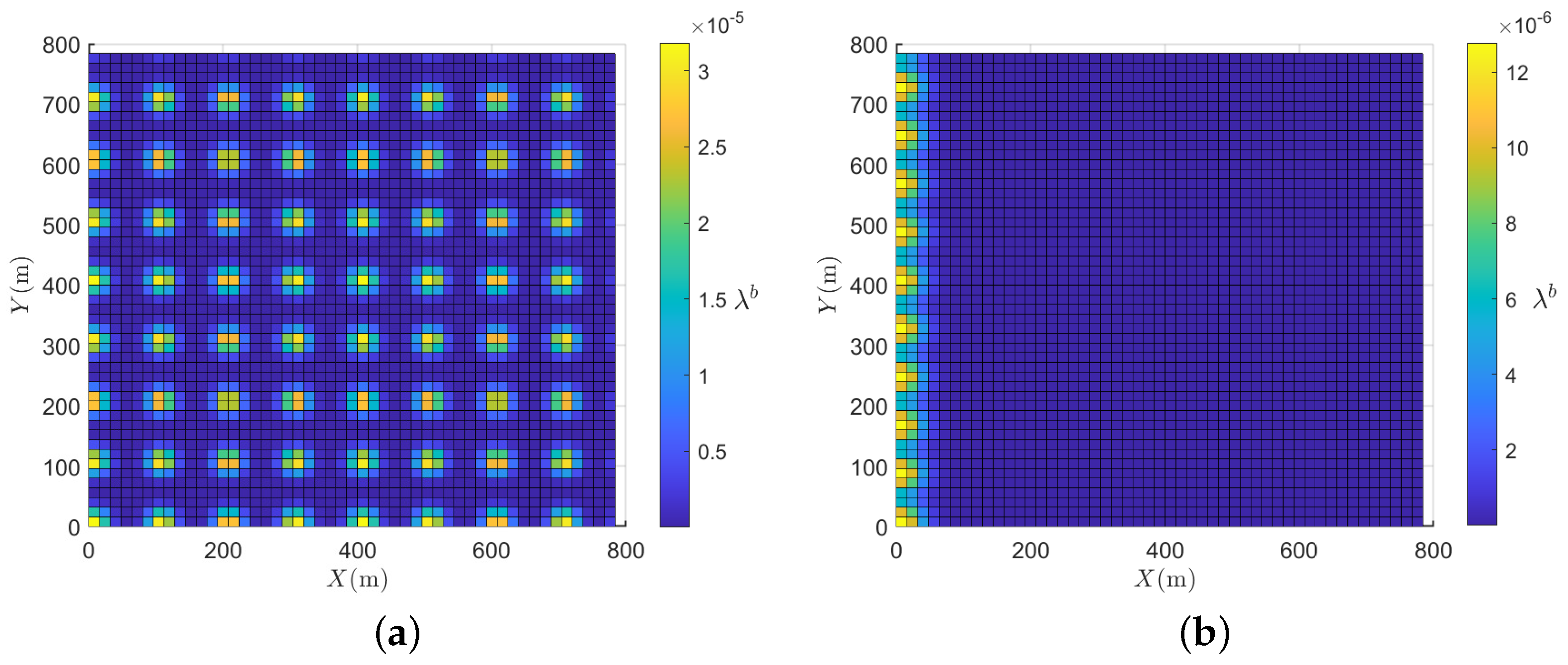
As the prior information of the target position could not be obtained in general, it was assumed that the possible birth positions of the targets were evenly distributed throughout the whole search area. As shown in Figure 3a, the Poisson birth intensity was described by a Gaussian mixture ${\lambda }_k^b\left(x\right)={\sum }_{t=1}^{N_k^b}{w}_k^{b,t}\mathcal{N}\left(x;{\mu }_k^{b,t},P_k^{b,t}\right)$, with $N_k^b=81$. We assumed that a new target appeared every five frames; therefore, the weights of the Gaussian components were determined by $w_k^{b,t}=0.2/N_k^b=3.1\times {10}^{-3},t\in \left[1,N_k^b\right]$. The mean of the Gaussian components was ${\mu }_k^{b,t}={\left[p_x^i,0,p_y^i,0\right]}^T$, where $p^i\in \{0\mathrm{m},100\mathrm{m},\dots ,800\mathrm{m}\}\times \{0\mathrm{m},100\mathrm{m},\dots ,800\mathrm{m}\}$. The covariance matrix of the birth intensity was $P_k^{b,t}=\mathrm{diag}{\left([200,5,200,5]\right)}^2$. The initial value of the unknown target intensity was set to be the same as ${\lambda }_k^b\left(x\right)$. The weight in the objective function was set to be $\eta =2$.

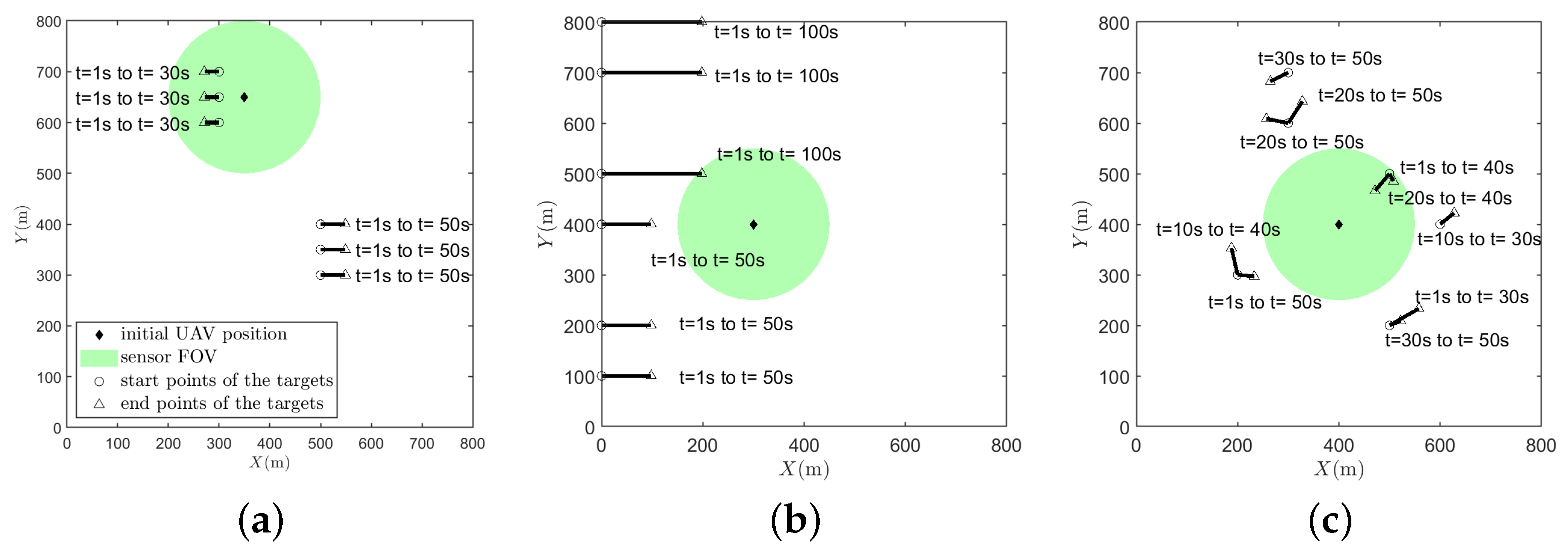
To verify the performance of the proposed UAV trajectory optimization algorithm in target search and tracking applications, three simulation scenarios were set, as shown in Figure 4. In the figures, the black diamonds were the initial positions of the four UAVs, and the green circular area represented the FOVs of the sensors. The black solid lines were the trajectories of the targets without considering the process noise. The hollow circles stood for the starting position of the tracks, while the hollow triangles stood for the termination positions. The time labels in the figures demonstrated the appearing and disappearing time instants of the corresponding target in the search area. The three simulation scenarios are described in detail as follows:

Scenario 1: Opposite-moving. As shown in Figure 4a, the initial position of the UAVs is $(350\mathrm{m},650\mathrm{m})$, and there are two groups of targets moving in opposite directions from the initial moment, one of which is within the FOVs of the sensors. The setting of this scenario aimed to investigate whether the proposed trajectory optimization method can explore and find potential targets successfully, while maintaining the tracking accuracy of the discovered targets.

Scenario 2: Prior-information. This scenario considers special scenarios with prior information about the target birth, such as a scenario where ground vehicles cannot cross obstacles and where the range of entrance is limited. As shown in Figure 3b, assuming that the targets can only enter the area through the left edge of the area, the parameters in the birth intensity model ${\lambda }_k^b\left(x\right)={\sum }_{t=1}^{N_k^b}{w}_k^{b,t}\mathcal{N}\left(x;{\mu }_k^{b,t},P_k^{b,t}\right)$ are given by $N_k^b=11$, and the Gaussian components distribute evenly on the left edge. The mean value of the position components is $p^i\in 0\mathrm{m}\times \{0\mathrm{m},100\mathrm{m},\dots ,800\mathrm{m}\}$. The scenario is shown in Figure 4b. Six targets enter the search area from the left edge at the initial instant, and the initial position of the UAVs is $(300\mathrm{m},400\mathrm{m})$. The setting of this scenario aims to examine whether the proposed trajectory optimization algorithm can keep track of the discovered target while searching a region with high unknown target density.

Scenario 3: Random-appearing. As shown in Figure 4c, there are four UAVs searching and tracking for 10 targets, with no prior information of target birth. The 10 targets appear in the search area randomly, and the initial position of the UAVs is $(400\mathrm{m},400\mathrm{m})$. The setting of this scenario is intended to comprehensively test the ability of the trajectory optimization algorithm to search and track multiple targets.

5.3. Simulation Results

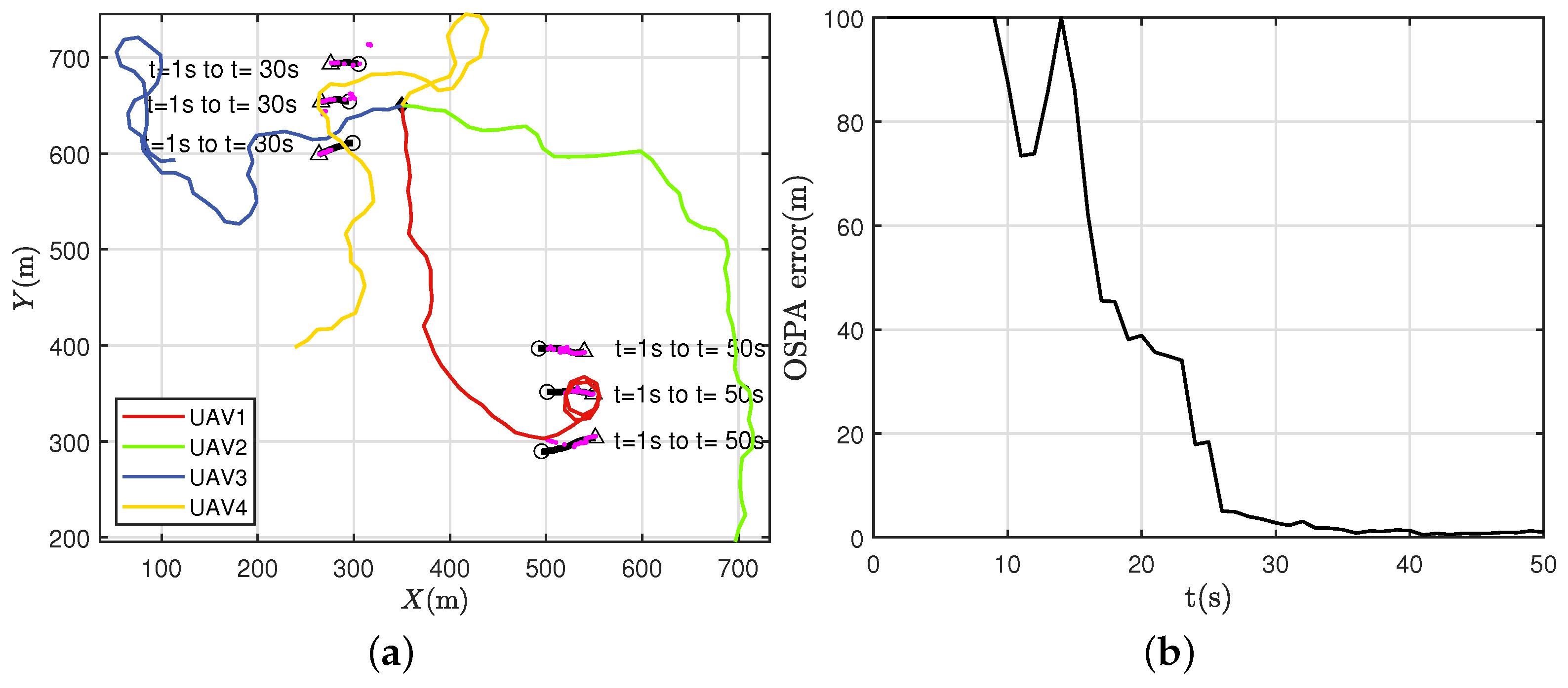
The simulation results of Scenario 1 are shown in Figure 5. Figure 5a presents the trajectories optimization results of the four UAVs, where the purple scattering points are the target positions estimated by the multi-sensor multi-target tracking algorithm. Figure 5b presents the OSPA error of the multi-target positions. It can be seen from the figure that although initially there was one group of targets covered by the sensor FOV, two UAVs, with trajectories in red and green, moved towards the bottom right of the search area, to balance the search and tracking objectives. Then, the UAV with the red trajectory discovered the second group of targets, from $t=15\mathrm{s}$ to $t=25\mathrm{s}$, and kept track of them. The UAV with the green trajectory continued to search for the potential targets in the unexplored area, and the second group of targets never appeared in its FOV. When $t=30\mathrm{s}$, the three targets in the upper-left corner disappeared, and the UAVs with the blue and yellow trajectories started to explore other regions. From the simulation results of Scenario 1, it can be seen that the proposed trajectory optimization algorithm can well balance the two purposes of target search and tracking.

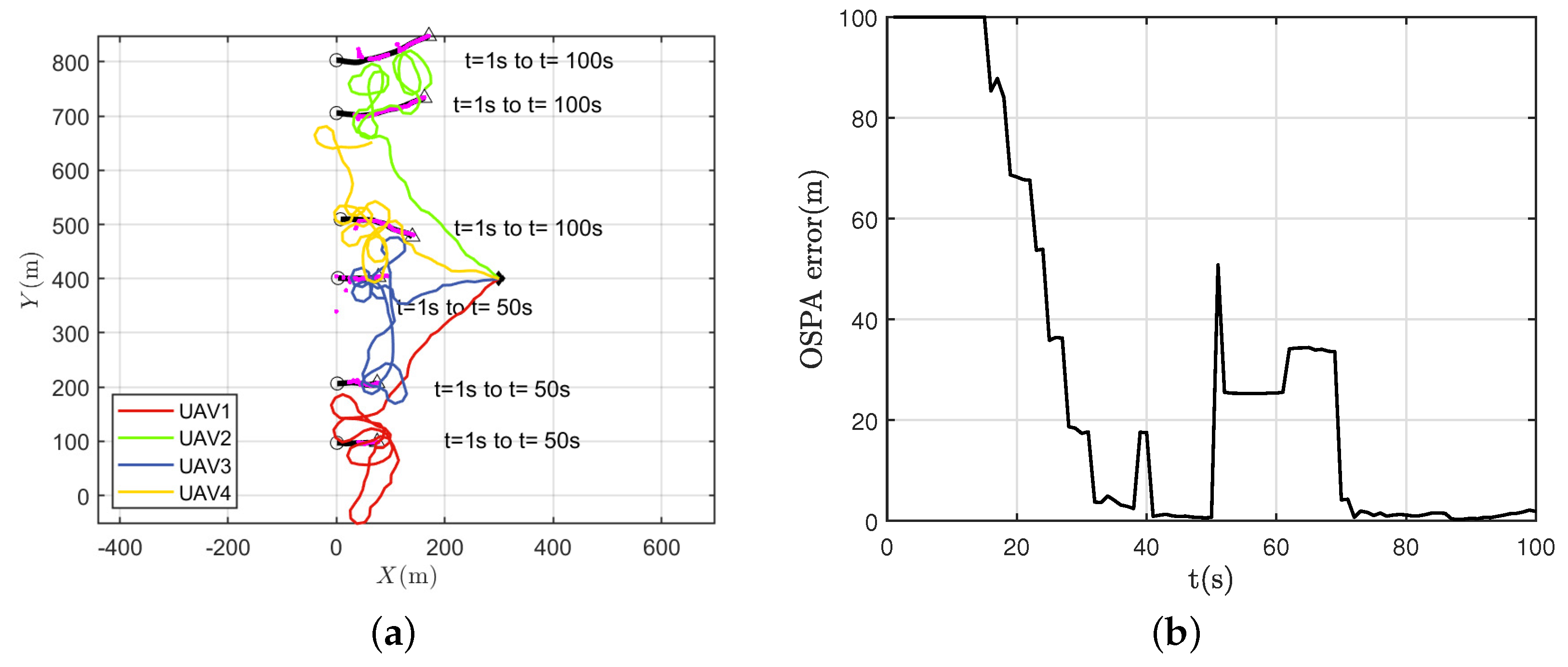
Figure 6 shows the simulation results of Scenario 2. As there was no target in the sensor FOV of the four UAVs, they moved towards the left, where the intensity of unknown targets was high for searching purposes. From Figure 6b, it can be seen that the six targets from the left edge were confirmed by the UAVs successively between $t=15\mathrm{s}$ and $t=30\mathrm{s}$, and that the OSPA error remained below $20\mathrm{m}$. When $t=50\mathrm{s}$, the three targets in the lower half of the region disappeared. As the termination of targets needed to be confirmed, based on a series of subsequent measurements, the OSPA error corresponding to this time increased. When $t=60\mathrm{s}$, in order to reduce the intensity of unknown targets in the longitudinal range of $600\mathrm{m}$ to $700\mathrm{m}$, the UAV with the green trajectory began to move downwards, which resulted in the loss of the uppermost target. Five seconds later, the FOV of the UAV with the yellow trajectory covered this area, and the green one returned to the top area and kept track of the two targets. The results revealed that the trajectory optimization algorithm can track the discovered targets while monitoring the regions with high unknown target intensity by coordinating the UAV team, ensuring that the overall tracking error is within an acceptable range.

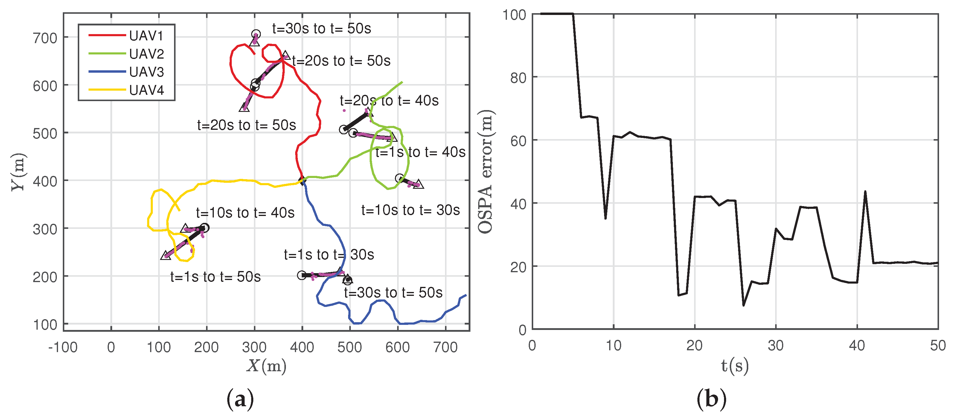
The simulation results of Scenario 3 are presented in Figure 7. It can be seen from Figure 7a that the target at $(500\mathrm{m},500\mathrm{m})$ was located within the detection range of the four UAVs. To balance the performance of search and tracking, the two UAVs with the red and green trajectories moved towards this target, to reduce the tracking error. The other two UAVs flew towards the rest part of the field, to search for more potential targets. The UAV with the trajectory in red detected the target at $(300\mathrm{m},600\mathrm{m})$ while tracking the first target discovered, and it moved to the newly discovered one, while the second UAV kept track of the first target. The UAV with the yellow trajectory successively initiated the two targets at $(200\mathrm{m},300\mathrm{m})$, and it maintained high tracking accuracy. Note that the UAV with the blue trajectory failed to initiate the target appearing at $30 \mathrm{s}$, as it was close to another target terminating at $(500\mathrm{m},200\mathrm{m})$, which is an inherent flaw of the JPDA-based multi-target tracking approaches. Figure 7b shows the OSPA error of the multi-target positions. It can be seen that the OSPA error converged well and that the sharp increases corresponded to the time of target birth or termination. This is because the initiation of new targets and the confirmation target disappearance need to be determined by multi-frame sensor measurements.

6. Conclusions

A trajectory optimization algorithm for multi-target search and tracking with airborne bearing sensors is proposed in this paper. The intensity of unknown targets is modeled and updated according to the UAV trajectory, guiding the UAVs towards the area with high unknown target intensity. The intensity of unknown targets is also considered in the calculation of external density in the JIPDA algorithm, which facilitates the initiation of potential targets. According to the predicted posterior unknown target intensity and the posterior tracking error covariance of the existing targets, an integrated dimensionless evaluation criterion is created. By leveraging the criterion as the objective function, the UAV trajectory optimization problem is constructed. Numerical simulations in different tracking scenarios were performed, to validate the proposed approach. The simulation results showed that in opposite-moving and prior-information scenarios the UAVs discovered all the targets in the region of interest and that the OSPA error converged to less than 3 m. In the random-appearing scenario, the steady value of the OSPA error was maintained at around 20 m, due to the close-spacing targets. The results demonstrate that the proposed trajectory optimization method balances the search and tracking objectives well and that it maintains acceptable multi-target tracking accuracy.

References

1. Kim, H.; Mokdad, L.; Ben-Othman, J. Designing UAV surveillance frameworks for smart city and extensive ocean with differential perspectives. IEEE Commun. Mag. 2018, 56, 98–104. [Google Scholar] [CrossRef]
2. Erdos, D.; Erdos, A.; Watkins, S.E. An experimental UAV system for search and rescue challenge. IEEE Aerosp. Electron. Syst. Mag. 2013, 28, 32–37. [Google Scholar] [CrossRef]
3. Wang, Y.; Bai, P.; Liang, X.; Wang, W.; Zhang, J.; Fu, Q. Reconnaissance mission conducted by UAV swarms based on distributed PSO path planning algorithms. IEEE Access 2019, 7, 105086–105099. [Google Scholar] [CrossRef]
4. Samir Labib, N.; Danoy, G.; Musial, J.; Brust, M.R.; Bouvry, P. Internet of unmanned aerial vehicles—A multilayer low-altitude airspace model for distributed UAV traffic management. Sensors 2019, 19, 4779. [Google Scholar] [CrossRef] [PubMed] [Green Version]
5. Minaeian, S.; Liu, J.; Son, Y.J. Vision-based target detection and localization via a team of cooperative UAV and UGVs. IEEE Trans. Syst. Man Cybern. Syst. 2015, 46, 1005–1016. [Google Scholar] [CrossRef]
6. Milan, A.; Rezatofighi, S.H.; Dick, A.; Reid, I.; Schindler, K. Online multi-target tracking using recurrent neural networks. In Proceedings of the AAAI Conference on Artificial Intelligence, San Francisco, CA, USA, 4–9 February2017; Volume 31. [Google Scholar]
7. Blackman, S.S. Multiple hypothesis tracking for multiple target tracking. IEEE Aerosp. Electron. Syst. Mag. 2004, 19, 5–18. [Google Scholar] [CrossRef]
8. He, S.; Shin, H.S.; Tsourdos, A. Trajectory optimization for target localization with bearing-only measurement. IEEE Trans. Robot. 2019, 35, 653–668. [Google Scholar] [CrossRef] [Green Version]
9. Nardone, S.C.; Aidala, V.J. Observability criteria for bearings-only target motion analysis. IEEE Trans. Aerosp. Electron. Syst. 1981, AES-17, 162–166. [Google Scholar] [CrossRef]
10. He, S.; Shin, H.S.; Xu, S.; Tsourdos, A. Distributed estimation over a low-cost sensor network: A review of state-of-the-art. Inf. Fusion 2020, 54, 21–43. [Google Scholar] [CrossRef]
11. Charrow, B.; Michael, N.; Kumar, V. Active control strategies for discovering and localizing devices with range-only sensors. In Algorithmic Foundations of Robotics XI: Selected Contributions of the Eleventh International Workshop on the Algorithmic Foundations of Robotics; Springer: Berlin/Heidelberg, Germany, 2015; pp. 55–71. [Google Scholar]
12. Dames, P.M. Distributed multi-target search and tracking using the PHD filter. Auton. Robot. 2020, 44, 673–689. [Google Scholar] [CrossRef] [Green Version]
13. Boström-Rost, P.; Axehill, D.; Hendeby, G. Sensor management for search and track using the Poisson multi-Bernoulli mixture filter. IEEE Trans. Aerosp. Electron. Syst. 2021, 57, 2771–2783. [Google Scholar] [CrossRef]
14. Boström-Rost, P.; Axehill, D.; Hendeby, G. PMBM filter with partially grid-based birth model with applications in sensor management. IEEE Trans. Aerosp. Electron. Syst. 2021, 58, 530–540. [Google Scholar] [CrossRef]
15. Van Nguyen, H.; Vo, B.N.; Vo, B.T.; Rezatofighi, H.; Ranasinghe, D.C. Multi-objective multi-agent planning for discovering and tracking unknown and varying number of mobile objects. arXiv 2022, arXiv:2203.04551. [Google Scholar]
16. Musicki, D.; Evans, R. Joint integrated probabilistic data association: JIPDA. IEEE Trans. Aerosp. Electron. Syst. 2004, 40, 1093–1099. [Google Scholar] [CrossRef]
17. He, S.; Shin, H.S.; Tsourdos, A. Trajectory optimization for multitarget tracking using joint probabilistic data association filter. J. Guid. Control Dyn. 2020, 43, 170–178. [Google Scholar] [CrossRef]
18. He, S.; Shin, H.S.; Tsourdos, A. Information-theoretic joint probabilistic data association filter. IEEE Trans. Autom. Control 2020, 66, 1262–1269. [Google Scholar] [CrossRef]
19. Williams, J.L. Marginal multi-Bernoulli filters: RFS derivation of MHT, JIPDA, and association-based MeMBer. IEEE Trans. Aerosp. Electron. Syst. 2015, 51, 1664–1687. [Google Scholar] [CrossRef] [Green Version]
20. He, S.; Shin, H.S.; Tsourdos, A. Multi-sensor multi-target tracking using domain knowledge and clustering. IEEE Sens. J. 2018, 18, 8074–8084. [Google Scholar] [CrossRef] [Green Version]
21. Bar-Shalom, Y.; Campo, L. The effect of the common process noise on the two-sensor fused-track covariance. IEEE Trans. Aerosp. Electron. Syst. 1986, AES-22, 803–805. [Google Scholar] [CrossRef]
22. Battistelli, G.; Chisci, L. Kullback–Leibler average, consensus on probability densities, and distributed state estimation with guaranteed stability. Automatica 2014, 50, 707–718. [Google Scholar] [CrossRef]
23. LeGrand, K.A.; Ferrari, S. Split Happens! Imprecise and Negative Information in Gaussian Mixture Random Finite Set Filtering. arXiv 2022, arXiv:2207.11356. [Google Scholar]
24. DeMars, K.J.; Bishop, R.H.; Jah, M.K. Entropy-based approach for uncertainty propagation of nonlinear dynamical systems. J. Guid. Control Dyn. 2013, 36, 1047–1057. [Google Scholar] [CrossRef]
25. Schuhmacher, D.; Vo, B.T.; Vo, B.N. A consistent metric for performance evaluation of multi-object filters. IEEE Trans. Signal Process. 2008, 56, 3447–3457. [Google Scholar] [CrossRef] [Green Version]
26. Challa, S. Fundamentals of Object Tracking; Cambridge University Press: Cambridge, UK, 2011. [Google Scholar]
Figure 1. Multi-UAV multi-target search and tracking scenario.
Aerospace 10 00652 g001
Figure 2. The intensity of unknown targets.
Aerospace 10 00652 g002
Figure 3. Distribution of the intensity of new targets in the search region. (a) Without prior birth information. (b) With prior birth information.
Aerospace 10 00652 g003
Figure 4. Multi-target search and tracking scenarios. (a) Scenario 1. (b) Scenario 2. (c) Scenario 3.
Aerospace 10 00652 g004
Figure 5. Simulation results of Scenario 1. (a) Trajectory optimization results. (b) OSPA error of position estimation.
Aerospace 10 00652 g005
Figure 6. Simulation results of Scenario 2. (a) Trajectory optimization results. (b) OSPA error of position estimation.
Aerospace 10 00652 g006
Figure 7. Simulation results of Scenario 3. (a) Trajectory optimization results. (b) OSPA error of position estimation.
Aerospace 10 00652 g007
Disclaimer/Publisher’s Note: The statements, opinions and data contained in all publications are solely those of the individual author(s) and contributor(s) and not of MDPI and/or the editor(s). MDPI and/or the editor(s) disclaim responsibility for any injury to people or property resulting from any ideas, methods, instructions or products referred to in the content.