Modeling and Control for an Aero-Engine Based on the Takagi-Sugeno Fuzzy Model

Abstract

This paper presents a study on the modeling and control of an aero-engine within the full flight envelope using the Takagi–Sugeno (T-S) fuzzy theory. A highly accurate aero-engine small deviation state variable model (SVM) was developed using the adaptive differential evolution, based on numerous successes through history, with the linear population size reduction (L-SHADE) algorithm. The affinity propagation (AP) clustering algorithm was then implemented to realize the division of flight envelopes based on the gap metric between the SVMs at each working point. By solving the membership parameters using the L-SHADE algorithm, the T-S fuzzy model was obtained, which has flight conditions as premises and engine linear SVM as consequences. Furthermore, based on the established T-S fuzzy model and T-S control theory, a controller design method is proposed. The simulation results show that the T-S fuzzy model has high accuracy and good generalization capability within the flight envelope, and the proposed control method can guarantee the asymptotic stability of the system, subject to external disturbance and time delay.

1. Introduction

The inherently nonlinear nature of aero-engines presents a challenge when applying existing nonlinear control theories to this complex system. As a result, most accepted approaches rely on linear systems theory for aero-engine control theory [1,2,3]. However, this requires the nonlinear models to be transformed into linear forms that are more amenable for analysis and control design, which can be a daunting task.

The prevailing methodology for aero-engine control theory involves linearizing the nonlinear model at its steady-state point to obtain a small deviation state variable model (SVM). Various approaches have been suggested in the literature, such as Sugiyama’s partial derivative method [4] that employs nonlinear dynamic simulation to solve the system matrix. However, it neglects variable coupling and leads to considerable modeling errors. Lin et al. [5] proposed a least square fitting method that enhances modeling accuracy, although its complex analytic relational formulas limit its application in higher-order object modeling. In contrast, Wang et al. [6] used the particle swarm optimization (PSO) algorithm to optimize the parameter matrices of an aero-engine SVM. This approach transforms the modeling problem into a parametric optimization problem, where the modeling accuracy mainly relies on the optimization algorithm’s superiority. Therefore, selecting an appropriate optimization algorithm can considerably enhance modeling accuracy and computational speed, making this approach highly promising for aero-engine modeling.

However, aero-engine dynamic characteristics vary significantly over a wide flight envelope, rendering the SVM obtained through the aforementioned method appropriate only for studying the dynamic characteristics in a small range around the steady-state point. It is unsuitable for the full flight envelope [7]. To address this issue, the Takagi–Sugeno (T-S) fuzzy model is regarded as a promising solution.

The T-S fuzzy model developed by Takagi and Sugeno [8] offers a notable advantage as it can describe the nonlinear system and enable the investigation of its stability and controller design problems using linear control theory. Consequently, the T-S fuzzy model has garnered extensive attention in the aero-engine control field [9,10].

As an illustration, Cai et al. [11] proposed a T-S fuzzy model identification method for aero-engines using the least squares method and the back-propagation method. However, this method entails excessive calculation due to the simultaneous identification of the model structure and parameters. In light of this, Wang et al. [12] proposed a modeling method based on the flight envelope division that derives the model antecedent structure through division by the flight envelope and the model consequent from the nominal point model, thereby considerably reducing computational effort. Nonetheless, this method uses generalized Euclidean distance within the flight envelope as the basis for flight envelope division, which is relatively crude and unable to describe the model differences at different operating points. Hence, Xu et al. [13] created characteristic parameters for aero-engines based on the dominant eigenvalues of the system matrix and the gain matrix of the transfer function, which they used as the basis for flight envelope division to attain a full flight envelope T-S fuzzy model. However, the method of representing system dynamics using the dominant eigenvalues of the system matrix can generate satisfactory results when the number of system states is small; otherwise, it is easy to neglect a lot of significant information and affect the flight envelope classification result.

The gap metric is a systematic metric concept distinct from the parametric metric that Zames and El-Sakkary introduced to the control field as a means of studying system uncertainty [14,15]. El-Sakkary’s research suggested that the gap metric is a more appropriate means of measuring the dissimilarity between two linear systems than parameter-based metrics and thus serves as a suitable metric for evaluating the variance between linear systems.

With the aforementioned discussion, this study introduces a novel approach to modeling aero-engine T-S fuzzy systems, addressing several significant challenges. First, we enhance the weak global search capability of the original L-SHADE algorithm using three mechanisms and propose a new SVM establishing method. Second, a novel flight envelope division method is proposed based on gap metric theory and the affinity propagation (AP) clustering algorithm to enhance the rationality of the approach. Third, we propose a new method of solving membership value using a membership matrix instead of the membership function, increasing the simplicity and accuracy of the modeling process. Finally, we present a new T-S fuzzy-model-based controller design approach for distributed systems to improve the verifiability of the T-S fuzzy model. Our proposed approach enables more effective, accurate, and verifiable modeling of aero-engine T-S fuzzy systems.

2. Description of the Aero-Engine T-S Fuzzy Model

Under non-afterburning conditions, aero-engines can generally be modeled as

$$\{\begin{array}{l}{\dot{n}}_L=f_1\left(n_L,n_H,W_f,A_8,{T_1}^{*},{P_1}^{*}\right)\\ {\dot{n}}_H=f_2\left(n_L,n_H,W_f,A_8,{T_1}^{*},{P_1}^{*}\right)\\ Y=f_3\left(n_L,n_H,W_f,A_8,{T_1}^{*},{P_1}^{*}\right)\end{array}$$

(1)

where $n_L$ and $n_H$ denote the low-pressure and high-pressure rotor speeds of the aero-engine, respectively. $W_f$ represents the main fuel flow, $A_8$ indicates the area of exit nozzle throat. ${T_1}^{*}$ and ${P_1}^{*}$ are the total inlet temperature and the total inlet pressure respectively. $Y$ represents the desired output of the aero-engine system.

The characteristics of an aero-engine depend on the total inlet temperature ${T_1}^{*}$ and pressure ${P_1}^{*}$ when the engine operating condition is determined. If the inlet is predetermined, ${T_1}^{*}$ and ${P_1}^{*}$ are only related to the flight height $H$ and Mach number $Ma$. Thus, if the engine operating and flight conditions are given, the incremental form state-space model of the aero-engine can be established as follows:

$$\{\begin{array}{c}\dot{x}\left(t\right)=Ax\left(t\right)+Bu\left(t\right)\\ y\left(t\right)=Cx\left(t\right)+Du\left(t\right)\end{array}$$

(2)

where $x={\left[\begin{array}{cc}\Delta n_L& \Delta n_H\end{array}\right]}^T$, $u={\left[\begin{array}{cc}\Delta W_f& \Delta A_8\end{array}\right]}^T$, $y$ can be specified as required, and in this paper, we define $y={\left[\begin{array}{cccc}\Delta n_L& \Delta n_H& \Delta P_3& \Delta T_5\end{array}\right]}^T$, where $P_3$ is the compressor delivery pressure, $T_5$ is the low-pressure turbine outlet temperature. To simplify the description in later sections, we will omit the incremental notation $\Delta$. The system matrix can be expressed as follows:

$$A=\left[\begin{array}{cc}{a}_{11}& a_{12}\\ a_{21}& a_{22}\end{array}\right], B=\left[\begin{array}{cc}{b}_{11}& b_{12}\\ b_{21}& b_{22}\end{array}\right], C=\left[\begin{array}{cc}1& 0\\ 0& 1\\ c_{11}& c_{12}\\ c_{21}& c_{22}\end{array}\right], D=\left[\begin{array}{cc}0& 0\\ 0& 0\\ d_{11}& d_{12}\\ d_{21}& d_{22}\end{array}\right]$$

Based on the above analysis, the T-S fuzzy model of an aero-engine in a particular operating condition (non-afterburning) within the full flight envelope can be expressed as follows:

$$\begin{array}{c}{\mathrm{R}}^i:\mathrm{if} H={\Psi }_{1i}\mathrm{and}Ma={\Psi }_{2i},\mathrm{then}\\ \{\begin{array}{c}\dot{x}\left(t\right)=A_{i}x\left(t\right)+B_{i}u\left(t\right)\\ y\left(t\right)=C_{i}x\left(t\right)+D_{i}u\left(t\right)\end{array}\end{array}$$

(3)

where ${\mathrm{R}}^i\left(i=1,2,\cdots ,r\right)$ refers to the $i^{\mathrm{th}}$ fuzzy rule, ‘if’ indicates the model antecedent and ‘then’ represents the model consequent. The fuzzy premises are set as $H$ and $Ma$ with ${\Psi }_{1i}$ and ${\Psi }_{2i}$ denoting the antecedent fuzzy sets of $H$ and $Ma$, respectively. $A_i$, $B_i$, $C_i$, $D_i$ correspond to the parameters of the conclusion part of the $i^{\mathrm{th}}$ fuzzy rule.

Hence, combining all the fuzzy rules, the global fuzzy model can be expressed as below:

$$\{\begin{array}{c}\dot{x}\left(t\right)={\displaystyle \sum _{i=1}^r{\mu }_i}\left[A_{i}x\left(t\right)+B_{i}u\left(t\right)\right]\\ y\left(t\right)={\displaystyle \sum _{i=1}^r{\mu }_i}\left[C_{i}x\left(t\right)+D_{i}u\left(t\right)\right]\end{array}$$

(4)

where ${\mu }_i$ is the degree of membership function of the $i^{\mathrm{th}}$ fuzzy rule satisfying $0\le {\mu }_i\le 1$ and ${\displaystyle \sum _{i=1}^r{\mu }_i}=1$.

3. Aero-Engine Full Flight Envelope Modeling

To establish the T-S fuzzy model for the aero-engine, four elements need to be determined, namely the antecedent structure, antecedent parameters, consequent structure, and consequent parameters. Based on this philosophy, we propose the following method for modeling.

First, the range of the flight envelopes under study is determined, and a specific set of steady-state working points is selected. Next, the set of SVMs is obtained by traversing each working point. It is worth noting that a higher number of working points leads to better modeling accuracy, but also increases computational effort significantly.

Second, the gap metric is used as the similarity metric of each linear model, and the AP clustering algorithm is used to divide the flight envelope and obtain the appropriate number of clustering centers that help determine the model’s antecedent structure. The SVMs of the clustering centers are then used as the model consequent.

Finally, the modeling error is selected as the cost function, and the membership matrix can be solved based on the optimization algorithm to establish the T-S fuzzy model.

Next, we present the details of the above modeling method.

3.1. Small Deviation State Variable Modeling

The steady-state point’s SVM forms the basis of the full flight envelope model. This section explains the modeling process for a highly accurate SVM. Specifically, we discuss the method of computing the system matrix in Equation (2).

The modeling of an aero-engine involves an approximate solution procedure of a linear model for the actual system. Obtaining test data for the real aero-engine can be challenging, and nonlinear thermodynamic component level models (NCLM) of aero-engines can accurately simulate real turbofan engines with high precision and fidelity [16]. Accordingly, we adopt the output of the NCLM as the approximation object. In this article, building on the ideas proposed by Wang [6], we transform the problem of identifying the model into a parameter optimization problem, which is described as follows:

$$\begin{array}{c}\underset{\theta }{\min }J\left(\theta \right)\\ s.t.\theta \in \chi \end{array}$$

(5)

where the decision variable $\theta$ is set as the unknown parameters of the matrices in (2), i.e., $\theta =\left[a_{11},a_{12},a_{21},a_{22},b_{11},b_{12},b_{21},b_{22},c_{11},c_{12},c_{21},c_{22},d_{11},d_{12},d_{21},d_{22}\right]$, the objective function $J$ is defined as the deviation between the output of the aero-engine NCLM and that of SVM, i.e., $J={\Vert {\widehat{y}}_1\left(k\right)-{\overline{y}}_1\left(k\right)\Vert }^2+{\Vert {\widehat{y}}_2\left(k\right)-{\overline{y}}_2\left(k\right)\Vert }^2$, where $k$ is a bounded discrete sampling moment, ${\overline{y}}_1$ is the normalized sequence of the step response $y_1$ of the NCLM to 1% steady-state value $\delta W_f$ of the fuel flow, given by ${\overline{\mathit{y}}}_1=H_1{y}_1$ with $H_1=1/\delta W_f$. Similarly, ${\overline{\mathit{y}}}_2$ represents the normalized sequence of the step response $y_2$ of the NCLM to 1% steady-state value $\delta A_8$ of the area of exit nozzle throat, given by ${\overline{\mathit{y}}}_2=H_2{y}_2$ with $H_2=1/\delta A_8$. ${\widehat{\mathit{y}}}_1$ and ${\widehat{\mathit{y}}}_2$ denote the step responses of the SVM to ${\overline{\mathit{u}}}_1={\left[\begin{array}{cc}1& 0\end{array}\right]}^T$ and ${\overline{\mathit{u}}}_2={\left[\begin{array}{cc}0& 1\end{array}\right]}^T$, respectively. $\chi$ is the given feasible region.

When multiple parameters require optimization, the search space can grow larger, which slows down the algorithm convergence. In order to enhance optimization efficiency, a stepwise optimization approach in combination with the model structure can be utilized to decompose a smaller optimization problem within the larger optimization problem (5). First, the optimization algorithm is employed to solve the smaller optimization problem, which ultimately yields an optimized solution. This optimized solution serves as the initial value for optimizing the larger problem (5) and, finally, the optimization algorithm is applied to solve the entire optimization problem.

The decomposed optimization problem can be described as follows:

$$\begin{array}{c}\underset{{\theta }_1}{\min }{J}_1\left({\theta }_1\right)\\ s.t.{\theta }_1\in \chi \\ {\theta }_1=\left[a_{11},a_{12},a_{21},a_{22},b_{11},b_{12},b_{21},b_{22}\right]\\ J_1={\displaystyle \sum _{j=1}^2\left[{\displaystyle \sum _{k=1}^N{\left({\overline{n}}_{Lj}\left(k\right)-{\widehat{n}}_{Lj}\left(k\right)\right)}^2+{\displaystyle \sum _{k=1}^N{\left({\overline{n}}_{Hj}\left(k\right)-{\widehat{n}}_{Hj}\left(k\right)\right)}^2}}\right]}\end{array}$$

(6)

where $N$ refers to the total amount of sampling numbers, ${\overline{n}}_{Lj}$ and ${\overline{n}}_{Hj}$ designate $n_L$ and $n_H$ in the output ${\overline{\mathit{y}}}_{\mathrm{j}}$ of the NCLM, respectively. Meanwhile, ${\widehat{n}}_{Lj}$ and ${\widehat{n}}_{Hj}$ refer to $n_L$ and $n_H$ in the output ${\widehat{\mathit{y}}}_{\mathrm{j}}$ of the SVM.

Upon transforming the modeling problem into a parameter optimization problem, the accuracy of the model heavily relies on the optimization algorithm’s ability to find the optimal solution. Metaheuristic algorithms are a useful tool for discovering optimal values, and among them, adaptive differential evolution, based on numerous successes through history, with linear population size reduction (L-SHADE) has demonstrated excellent performance in various optimization problems [17]. Therefore, this section focuses on utilizing L-SHADE to perform parameter optimization and determine the optimal values of unknown model parameters. As this algorithm has been studied extensively in previous works, we will not provide a detailed explanation here. Readers can refer to [18] for more information.

However, the population linear reduction strategy of the algorithm may impact the population diversity when the initial population shrinks rapidly, leading to getting trapped in the local optimum solution. In the face of complex problems, L-SHADE algorithm performance may be affected. To address this issue, three mechanisms are implemented to enhance the performance of the original L-SHADE algorithm and improve the modeling results.

The first modification involves implementing an opposition-based learning strategy [19] for population initialization to produce high-quality initial populations. Conventional initial populations are often generated using a random distribution mechanism, resulting in an uneven distribution in the solution space and a lack of diversity in the initial population. In this study, a population initialization approach was proposed, which involves generating a set of candidate initial populations ${\mathit{p}}_0^{\mathbf{\prime }}$, followed by generating a complementary set of populations according to ${\mathit{p}}_0^{\mathbf{″}}=p_{\max }+p_{\min }-{\mathit{p}}_0^{\mathbf{\prime }}$. The fitness of each individual in the candidate populations and their complementary sets is then calculated, and the top-performing individuals are selected to form the final initial population $p_0$.

The second enhancement involves updating the strategy for managing out-of-bounds individuals. In the L-SHADE algorithm, some individuals may exceed the boundary due to the mutation operation. To address this, we propose generating comparatively better solutions to replace the out-of-bounds individuals based on the top-performing individuals in the original population. The specific method is outlined below:

$$v_{inew,g}^j=\{\begin{array}{cc}0.5\cdot \left(p_{\max }^j+p_{pbest,g}^j\right)& if{v}_i^j>p_{\max }^j\\ 0.5\cdot \left(p_{\min }^j+p_{pbest,g}^j\right)& if{v}_i^j<p_{\min }^j\end{array}$$

(7)

where $v_i^j$ represents the $j^{\mathrm{th}}$ parameter value of the $i^{\mathrm{th}}$ individual. $p_{\max }^j$ and $p_{\min }^j$ correspond to the upper and lower bounds of the $j^{\mathrm{th}}$ parameter. $p_{pbest,g}^j$ denotes the $j^{\mathrm{th}}$ parameter value of an individual $p_{pbest,g}$, which is randomly selected from the current generation and ranks in the top $\left(p\times 100\right)\%$ of the fitness function. $v_{inew,g}^j$ represents the updated value of the out-of-bounds parameter.

The third enhancement involves optimizing the reduction mechanism. In the L-SHADE algorithm, a linear population reduction mechanism is adopted, resulting in a linear decrease of population size from the start of the iteration. This approach involves removing individuals that have not yet undergone evolution. This strategy reduces both population diversity and convergence speed, and if the initial population size is small, it may lead the algorithm to fall into locally optimal and premature convergence. To address this, we introduce a reduction margin $rm$. The population starts to decrease linearly only when a specific condition is met. Individuals with the lowest fitness rank are removed during the reduction process. The reduction model can be described as follows:

$$\begin{array}{c}N{P}_{g+1}=\{\begin{array}{cc}N{P}_g& ifFES/FE{S}_{\max }\le rm\\ N{P}^{\prime }& ifFES/FE{S}_{\max }>rm\end{array}\\ N{P}^{\prime }=round\left[N{P}_0-\frac{FES}{FE{S}_{\max }}\cdot \frac{\left(N{P}_0-N{P}_{\min }\right)}{\left(1-rm\right)}\right]\end{array}$$

(8)

where $N{P}_g$ represents the population size of the $g^{\mathrm{th}}$ generation, $FES$ and $FE{S}_{\max }$ denote the current and maximum number of times the fitness function is evaluated, respectively.

3.2. Flight Envelope Division

To determine the antecedent structure of the T-S fuzzy model, the flight envelope needs to be divided into several regions based on the effect of $H$ and $Ma$ on the aero-engine. Here, we present the AP clustering algorithm based on the gap metric to achieve this goal.

In this paper, we aim to perform clustering on $n$ steady-state working points in the study region. We define the study region as $E=\left\{E_1,E_2,\cdots ,E_{\mathrm{n}}\right\}$, where $E_i$ represents the $i^{\mathrm{th}}$ steady-state working point, characterized by $H_i$ and $M{a}_i$.

The AP clustering algorithm [15,20] gauges the similarity between data points to cluster them. To measure this similarity, we use the gap metric, which proves more adept at discerning differences between linear systems than the traditional Euclidean distance. We calculate the similarity between point $i$ and point $j$ as the negative value of the gap metric between the SVMs at the two points, that is,

$$S\left(i,j\right)=-\delta \left(M_i,M_j\right), i\ne j, i=1,2,\cdots ,n, j=1,2,\cdots ,n$$

(9)

where $S$ represents the similarity matrix. $M_i$ indicates the SVM of the point $i$. Meanwhile, $\delta \left(M_i,M_j\right)$ represents the gap between the model $M_i$ and $M_j$.

Remark 1.

The gap metric is a measure of the dissimilarity between two linear systems, with lower values indicating greater similarity in dynamic characteristics, and values closer to 1 indicating greater differences between the two systems. Due to space constraints, we cannot describe its definition in detail here, and readers can refer to [15].

The diagonal element $S\left(i,i\right)$ in the similarity matrix shows the fitness of point $i$ as a potential clustering center. The higher its value, the more suitable point $i$ is as a center. To ensure that each point has an equal likelihood of becoming a clustering center initially, the diagonal elements are set to the same value of the bias parameter $p$ when calculating $S$.

The key concept behind the AP clustering algorithm is the exchange of attractiveness $R$ and responsibility $A$ messages facilitated by the similarity matrix $S$. Through a series of iterative updates, the algorithm converges to a final set of clustering centers [12,15,20]. The workflow is illustrated below:

Step 1: Determine the similarity matrix $S$ and the bias parameter $p$. Set the attractiveness $R$ and the attribution $A$ to zero matrices that match the dimensions of $S$.

Step 2: Update the attractiveness $R$ using Equations (10) and (11).

$$R\left(i,k\right)=\{\begin{array}{l}S\left(i,k\right)-\underset{k^{\prime },k^{\prime }\ne k}{\max }\left\{A\left(i,k^{\prime }\right)+S\left(i,k^{\prime }\right)\right\},i\ne k\hfill \\ S\left(i,k\right)-\underset{k^{\prime },k^{\prime }\ne k}{\max }\left\{S\left(i,k^{\prime }\right)\right\},i=k\hfill \end{array}$$

(10)

$$R\left(i,k\right)=\left(1-\lambda \right)R\left(i,k\right)+\lambda R_{old}\left(i,k\right)$$

(11)

where $R$ is the current iteration value, $R_{old}$ is the last iteration value, $\lambda \in \left[0.5,1\right)$ represents the damping coefficient for ensuring algorithm convergence.

Step 3: Update the attribution $A$ using Equations (12) and (13).

$$A\left(i,k\right)=\{\begin{array}{l}\underset{k^{\prime },k^{\prime }\ne k}{\min }\left\{0,R\left(k,k\right)+{\displaystyle \sum _{i^{\prime },i^{\prime }\notin \left\{i,k\right\}}\max \left\{0,R\left(i^{\prime },k\right)\right\}}\right\},i\ne k\hfill \\ {\displaystyle \sum _{i^{\prime },i^{\prime }\notin \left\{i,k\right\}}\max \left\{0,R\left(i^{\prime },k\right)\right\}},i=k\hfill \end{array}$$

(12)

$$A\left(i,k\right)=\left(1-\lambda \right)A\left(i,k\right)+\lambda A_{old}\left(i,k\right)$$

(13)

where $A$ is the current iteration value, $A_{old}$ is the last iteration value.

Step 4: Calculate $R+A$ and take the working point $k$ with $R\left(k,k\right)+A\left(k,k\right)>0$ as a cluster center.

Step 5: Verify if the termination condition is satisfied; that is, if stable cluster centers have formed (the same centers are selected $t_{\mathrm{conv}}$ number of times), or if the maximum number of iterations $t_{\max }$ has been attained. If either of these conditions is not met, move back to step 2 to continue iterating.

Step 6: Assign all working points to the clustering centers based on the criterion of maximum similarity to obtain the final clustering outcomes.

3.3. Fuzzy Membership Solving

Through the previous procedure, we have established the model antecedent structure and the model consequent. The next step is to determine the membership values ${\mu }_i$$\left(i=1,2,\cdots r\right)$ for each fuzzy rule at any given working point within the flight envelope. The magnitude of the value denotes the amount of contribution of the rule to the final model at the respective working point.

The general method for determining the membership values is as follows. First, calculate the membership matrix for each rule $F={\left\{{\mu }_{ij}\right\}}_{r\times n}$ at each working point, where ${\mu }_{ij}$ denotes the membership value of the $j^{\mathrm{th}}$ working point for the $i^{\mathrm{th}}$ rule. Second, use the commonly employed membership functions to fit the membership sequences corresponding to different rules. For instance, to solve for the unknown parameters in the given formal membership functions ${\omega }_{H,i}$ and ${\omega }_{Ma,i}$, select the minimization of the error function ${\displaystyle \sum _{j=1}^n\left[{\mu }_{ij}-\Pi \left[{\omega }_{H,i}\left(H_j\right){\omega }_{Ma,i}\left(M{a}_j\right)\right]\right]}$ as the optimization objective for the $i^{\mathrm{th}}$ rule. Finally, compute the membership value of a specific working point based on the membership function determined.

Nonetheless, this paper considers the fact that when the commonly used membership function is utilized to fit the acquired membership sequence, it may unavoidably induce computational errors and lead to a decrease in the accuracy of the T-S fuzzy model. Therefore, the membership values of diverse working points for various rules are directly computed based on the obtained membership matrix. To fulfill the requirement of full flight envelope modeling, the membership values of the unassigned working points can be acquired through two-dimensional nearest neighbor interpolation.

The specific procedure for determining the membership matrix $F$ is as follows.

Step 1: Initialize the membership matrix $F=\mathbf{0}$.

Step 2: Combine the clustering outcomes and (4) to obtain a fuzzy model for given working points based on the obtained affiliation matrix $F$.

Step 3: Utilizing the methods introduced in Section 3.1, obtain the responses of the fuzzy model ${\widehat{\mathit{y}}}_1$ and ${\widehat{\mathit{y}}}_2$ as well as the responses of NCLM ${\overline{\mathit{y}}}_1$ and ${\overline{\mathit{y}}}_2$ for the same step inputs ${\overline{\mathit{u}}}_1$ and ${\overline{\mathit{u}}}_2$. The error function can be computed as $e={\Vert {\widehat{\mathit{y}}}_1-{\overline{\mathit{y}}}_1\Vert }^2+{\Vert {\widehat{\mathit{y}}}_2-{\overline{\mathit{y}}}_2\Vert }^2$.

Step 4: The proposed improved L-SHADE algorithm is utilized to determine the optimal value of the membership matrix that minimizes the cost function $J$. Hereby, considering that for any working point, it is necessary to ensure that ${\displaystyle \sum _{i=1}^r{\mu }_{ij}}=1\left(j=1,2,\cdots n\right)$, the cost function is therefore defined as below:

$$J=\alpha {\displaystyle \sum _{j=1}^n\left[{\left(1-{\displaystyle \sum _{i=1}^r{\mu }_{ij}}\right)}^2\right]}+e$$

(14)

where $\alpha$ denotes the weighting factor.

4. Aero-Engine Distributed System Controller Design

In order to verify the effectiveness of the work presented in this paper and facilitate the verification of whether the established T-S fuzzy model can replace the original model for controller design, this section proposes a methodology for designing controllers based on the T-S fuzzy model in an aero-engine partially distributed control system architecture [21].

According to the work in [7], considering the effect of systematic errors, the global fuzzy model (4) can be rewritten as below:

$$\{\begin{array}{l}\dot{\mathit{x}}\left(t\right)={\displaystyle \sum _{i=1}^r{\mu }_i}\left[A_{i}x\left(t\right)+B_{i}u\left(t\right)+w\left(t\right)\right]\hfill \\ y\left(t\right)={\displaystyle \sum _{i=1}^r{\mu }_i}\left[C_{i}x\left(t\right)+D_{i}u\left(t\right)\right]\hfill \end{array}$$

(15)

where $w\left(t\right)$ is the time-independent zero-mean white noise, and the rest of the parameters as defined in (4).

Given that all system states are accessible, this paper adopts state feedback fuzzy control rules as outlined below:

$$\begin{array}{c}{\mathrm{R}}^i:\mathrm{if}H={\Psi }_{1i}\mathrm{and}Ma={\Psi }_{2i},\mathrm{then}\\ u\left(t\right)=K_{i}x\left(t\right)\end{array}$$

(16)

where $K_i$ refers to the controller gain. By merging all the rules, the fuzzy controller derived from the fuzzy model can be expressed as follows:

$$u\left(t\right)={\displaystyle \sum _{i=1}^r{\mu }_i}{K}_{i}x\left(t\right)$$

(17)

In the distributed control system architecture, it is crucial to consider the impact of the network-induced delay brought by the communication network on the control system. Therefore, combining (15) and (17), the closed-loop system model with time delay can be expressed as follows:

$$\{\begin{array}{l}\dot{\mathit{x}}\left(t\right)={\displaystyle \sum _{i=1}^r{\displaystyle \sum _{j=1}^r{\mu }_i{\mu }_j\left[A_{i}x\left(t\right)+B_i{K}_{j}x\left(t-\tau \left(t\right)\right)+w\left(t\right)\right]}}\hfill \\ y\left(t\right)={\displaystyle \sum _{i=1}^r{\displaystyle \sum _{j=1}^r{\mu }_i{\mu }_j\left[C_{i}x\left(t\right)+D_i{K}_{j}x\left(t-\tau \left(t\right)\right)\right]}}\hfill \end{array}$$

(18)

where $\tau \left(t\right)$ is a bounded time delay that satisfies $0\le \tau \left(t\right)\le {\tau }_M$.

For ease of presentation, the following notation is defined. For a matrix $X$, $sym\left(X\right)$ refers to $X+X^T$ and $X>0$ indicates that $X$ is a symmetric positive definite matrix. $\ast$ symbolizes the symmetric term of the matrix. $I$ denotes the identity matrix with the appropriate dimension. Additionally, we define $e_i=\left[\begin{array}{ccc}{\mathbf{0}}_{i-1}& I& {\mathbf{0}}_{4-i}\end{array}\right]$$\left(i=1,2,3,4\right)$.

Theorem 1.

For the given delay parameters${\tau }_M>0$and tuning scalar$\rho$, if there exist matrices$X>0$,$\overline{Q}>0$,$\overline{R}>0$and$Y_j$,$1\le i<j\le r$, with appropriate dimensions such that inequalities (19) and (20) hold, then, the system (18) is asymptotically stable with an$H\infty$performance level$\gamma$, and the controller gain$K_j=Y_j{X}^{-1}$.

$$\left[\begin{array}{ccc}{\overline{\Pi }}_{ii}& \sqrt{{\tau }_M}{{\overline{\mathit{\Lambda }}}_{ii}}^T& {{\overline{\mathit{\Gamma }}}_{ii}}^T\\ *& {\rho }^2\overline{R}-2\rho X& 0\\ *& *& -I\end{array}\right]<0$$

(19)

$$\left[\begin{array}{ccccc}{\overline{\mathit{\Pi }}}_{ij}+{\overline{\mathit{\Pi }}}_{ji}& \sqrt{{\tau }_M}{{\overline{\mathit{\Lambda }}}_{ij}}^T& \sqrt{{\tau }_M}{{\overline{\mathit{\Lambda }}}_{ji}}^T& {{\overline{\mathit{\Gamma }}}_{ij}}^T& {{\overline{\mathit{\Gamma }}}_{ji}}^T\\ *& {\rho }^2\overline{R}-2\rho X& \mathbf{0}& \mathbf{0}& \mathbf{0}\\ *& *& {\rho }^2\overline{R}-2\rho X& \mathbf{0}& \mathbf{0}\\ *& *& *& -I& \mathbf{0}\\ *& *& *& *& -I\end{array}\right]<0$$

(20)

where   ${\overline{\mathit{\Pi }}}_{ij}={e_1}^T\left\{A_{i}X+X{A_i}^T+\overline{Q}-\overline{R}\right\}{e}_1-{e_2}^T\overline{\mathit{R}}{e}_2-{e_3}^T\overline{Q}{e}_3-{\gamma }^2{e_4}^T{e}_4+Sym\left\{{e_1}^T\left(B_i{Y}_j+\overline{\mathit{R}}\right)e_2+{e_1}^T{e}_4\right\}$,   ${\overline{\mathit{\Lambda }}}_{ij}=A_{i}X{e}_1+B_i{Y}_j{e}_2+e_4$, ${\overline{\mathit{\Gamma }}}_{ij}=C_{i}X{e}_1+D_i{Y}_j{e}_2$.

Proof of Theorem 1. 

Construct a Lyapunov–Krasovskii function candidate as follows:

$$V=x^T\left(t\right)Px\left(t\right)+{\displaystyle {\int }_{t-{\tau }_M}^t{x}^T\left(s\right)Qx\left(s\right)ds}+{\tau }_M{\displaystyle \underset{-{\tau }_M}{\overset{0}{\int }}{\displaystyle \underset{t+s}{\overset{t}{\int }}{\dot{x}}^T\left(v\right)R\dot{x}\left(v\right)dv}ds}$$

(21)

where $P$, $Q$, $R$ are all positive definite matrices with appropriate dimensions.

Calculating the derivative of (21) yields:

$$\begin{array}{ll}\dot{V}& =2x^T\left(t\right)P\dot{x}\left(t\right)+x^T\left(t\right)Qx\left(t\right)-x^T\left(t-{\tau }_M\right)Qx\left(t-{\tau }_M\right)+{\tau }_M{\dot{x}}^T\left(t\right)R\dot{x}\left(t\right)\\ & -{\tau }_M{\displaystyle \underset{t-{\tau }_M}{\overset{t}{\int }}{\dot{x}}^T\left(s\right)R\dot{x}\left(s\right)ds}\end{array}$$

(22)

For ease of expression, define ${\xi }^T\left(t\right)=\left[x^T\left(t\right),x^T\left(t-\tau \left(t\right)\right),x^T\left(t-{\tau }_M\right),w^T\left(t\right)\right]$.

Furthermore, by defining $J=\dot{V}\left(t\right)-{\gamma }^2{w}^T\left(t\right)w\left(t\right)+y^T\left(t\right)y\left(t\right)$, and combining it with Jessen’s inequality [22], we obtain the following:

$$\begin{array}{l}J\le {\xi }^T\left(t\right)\{{\displaystyle \sum _{i=1}^r{\displaystyle \sum _{j=1}^r{\mu }_i{\mu }_j\left\{2{e_1}^{T}P{\Lambda }_{ij}\right\}}}+{e_1}^T\left(t\right)Q{e}_1-{e_3}^{T}Q{e}_3+{\displaystyle \sum _{i=1}^r{\displaystyle \sum _{j=1}^r{\displaystyle \sum _{p=1}^r{\displaystyle \sum _{q=1}^r{\mu }_i{\mu }_j}}{\mu }_p{\mu }_q}}\left\{{\mathit{\tau }}_M{{\Lambda }_{ij}}^{T}R{\Lambda }_{pq}\right\}\\ \begin{array}{l}\hfill \end{array}-{\left[e_1-e_2\right]}^{T}R\left[e_1-e_2\right]-{\gamma }^2{e_4}^T{e}_4+{\displaystyle \sum _{i=1}^r{\displaystyle \sum _{j=1}^r{\displaystyle \sum _{p=1}^r{\displaystyle \sum _{q=1}^r{\mu }_i{\mu }_j}}{\mu }_p{\mu }_q}}\left\{{{\Gamma }_{ij}}^T{\Gamma }_{pq}\right\}\}\xi \left(t\right)\end{array}$$

(23)

where ${\Lambda }_{ij}=A_i{e}_1+B_i{K}_j{e}_2+e_4$, ${\Gamma }_{ij}=C_i{e}_1+D_i{K}_j{e}_2$.

According to Lemma 3 in [9], the following is obtained:

$$\begin{array}{l}{\displaystyle \sum _{i=1}^r{\displaystyle \sum _{j=1}^r{\displaystyle \sum _{p=1}^r{\displaystyle \sum _{q=1}^r{\mu }_i{\mu }_j}}{\mu }_p{\mu }_q}}\left\{{\tau }_M{{\Lambda }_{ij}}^{T}R{\Lambda }_{pq}\right\}\le {\displaystyle \sum _{i=1}^r{\displaystyle \sum _{j=1}^r{\mu }_i{\mu }_j}}\left\{{\tau }_M{{\Lambda }_{ij}}^{T}R{\Lambda }_{ij}\right\}\\ {\displaystyle \sum _{i=1}^r{\displaystyle \sum _{j=1}^r{\displaystyle \sum _{p=1}^r{\displaystyle \sum _{q=1}^r{\mu }_i{\mu }_j}}{\mu }_p{\mu }_q}}\left\{{{\Gamma }_{ij}}^T{\Gamma }_{pq}\right\}\le {\displaystyle \sum _{i=1}^r{\displaystyle \sum _{j=1}^r{\mu }_i{\mu }_j}}\left\{{{\Gamma }_{ij}}^T{\Gamma }_{ij}\right\}\end{array}$$

(24)

Furthermore, considering ${\displaystyle \sum _{i=1}^r{\displaystyle \sum _{j=1}^r{\mu }_i{\mu }_j}}\left\{{\Omega }_{ij}\right\}={\displaystyle \sum _{i=1}^r{{\mu }_i}^2}\left\{{\Omega }_{ii}\right\}+{\displaystyle \sum _{i=1}^r{\displaystyle \sum _{i<j}^r{\mu }_i{\mu }_j}}\left\{{\Omega }_{ij}+{\Omega }_{ji}\right\}$ and then combining (23) and (24), we obtain the following:

$$\begin{array}{l}J\le {\displaystyle \sum _{i=1}^r{{\mu }_i}^2}{\xi }^T\left(t\right)\left\{{\Pi }_{ii}+{\tau }_M{{\Lambda }_{ii}}^{T}R{\Lambda }_{ii}+{{\Gamma }_{ii}}^T{\Gamma }_{ii}\right\}\xi \left(t\right)+{\displaystyle \sum _{i=1}^r{\displaystyle \sum _{i<j}^r{\mu }_i{\mu }_j}}{\xi }^T\left(t\right)\{{\Pi }_{ij}+{\Pi }_{ji}+{\tau }_M{{\Lambda }_{ij}}^{T}R{\Lambda }_{ij}\\ \begin{array}{c}\end{array}+{\tau }_M{{\Lambda }_{ji}}^{T}R{\Lambda }_{ji}+{{\Gamma }_{ij}}^T{\Gamma }_{ij}+{{\Gamma }_{ji}}^T{\Gamma }_{ji}\}\xi \left(t\right)\end{array}$$

(25)

where ${\Pi }_{ij}=2{e_1}^{T}P{\Lambda }_{ij}+{e_1}^T\left(t\right)Q{e}_1-{e_3}^{T}Q{e}_3-{\left[e_1-e_2\right]}^{T}R\left[e_1-e_2\right]-{\gamma }^2{e_4}^T{e}_4$.

For $0\le {\mu }_i\le 1$, when (26) and (27) are simultaneously satisfied, $J\le 0$ is valid, indicating that the system (18) is asymptotically stable with an $H\infty$ performance.

$${\Pi }_{ii}+{\tau }_M{{\Lambda }_{ii}}^{T}R{\Lambda }_{ii}+{{\Gamma }_{ii}}^T{\Gamma }_{ii}<0$$

(26)

$${\Pi }_{ij}+{\Pi }_{ji}+{\tau }_M{{\Lambda }_{ij}}^{T}R{\Lambda }_{ij}+{\tau }_M{{\Lambda }_{ji}}^{T}R{\Lambda }_{ji}+{{\Gamma }_{ij}}^T{\Gamma }_{ij}+{{\Gamma }_{ji}}^T{\Gamma }_{ji}<0$$

(27)

Then, according to the Schur complement, Equations (26) and (27) is equivalent to

$$\left[\begin{array}{ccc}{\Pi }_{ij}& \sqrt{{\tau }_M}{{\Lambda }_{ij}}^{T}R& {{\Gamma }_{ij}}^T\\ *& -R& \mathbf{0}\\ *& *& -I\end{array}\right]<0$$

(28)

$$\left[\begin{array}{ccccc}{\Pi }_{ij}+{\Pi }_{ji}& \sqrt{{\tau }_M}{{\Lambda }_{ij}}^{T}R& \sqrt{{\tau }_M}{{\Lambda }_{ji}}^{T}R& {{\Gamma }_{ij}}^T& {{\Gamma }_{ji}}^T\\ *& -R& \mathbf{0}& \mathbf{0}& \mathbf{0}\\ *& *& -R& \mathbf{0}& \mathbf{0}\\ *& *& *& -I& \mathbf{0}\\ *& *& *& *& -I\end{array}\right]<\mathbf{0}$$

(29)

Define $X=P^{-1}$, ${\Gamma }_1=diag\left\{X,X,X,I,R^{-1},I\right\}$, ${\Gamma }_2=diag\left\{X,X,X,I,R^{-1},R^{-1},I,I\right\}$. Then, we multiply both left and right-hand sides of the inequality Equation (28) by ${\Gamma }_1$ and inequality Equation (29) by ${\Gamma }_2$. In addition, define $\overline{Q}=XQX$, $\overline{R}=XRX$, and $Y_j=K_{j}X$.

From the Lemma 3 in [23], it follows that for any scalar $\rho$, we have the following:

$$-R^{-1}=-X{\overline{R}}^{-1}X\le {\rho }^2\overline{R}-2\rho X$$

(30)

Thus, we conclude that if the LMIs (19) and (20) are feasible, then the system (18) is asymptotically stable. This completes the proof. □

5. Simulation and Analysis

To validate the proposed modeling and control method for the aero-engine full flight, envelope, simulations are conducted for a specific type of turbofan aero-engine using the modeling approach detailed in Section 3 and the control strategy outlined in Section 4.

5.1. Aero-Engine T-S Fuzzy Model

5.1.1. Small Deviation State Variable Modeling

The methodology proposed in this paper can be used to model an aero-engine within its entire flight envelope. However, since our objective in this section is to verify the method’s validity, we chose to validate the method by using a simplified flight envelope range, as shown in Figure 1a, which simplifies the overall modeling process. We then used 221 working points from within this selected flight envelope as training samples for the T-S fuzzy model, as illustrated in Figure 1b.

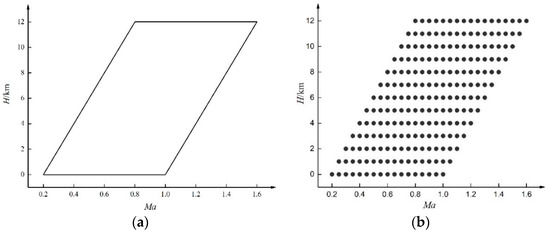
Figure 1. Selected operational range of aero-engine: (a) Selected flight envelope; (b) selected steady-state working points.

Initially, we evaluated the overall performance of the L-SHADE algorithm incorporating the hybrid strategy proposed in this paper. For this purpose, we selected the aero-engine at maximum power (non-afterburning) at $H=0 \mathrm{km}$, $Ma=0.2$ as our research object. We employed four representative algorithms: the multi-strategy improved L-SHADE algorithm (proposed in this paper), the genetic algorithm (GA), particle swarm optimization (PSO), and the basic L-SHADE algorithm, to solve the optimization problem Equation (6), and compared and analyzed the optimization results.

To ensure the fairness and accuracy of the experiments, we adopted a consistent hardware and software platform for all the algorithms tested and conducted simulations on a Windows 10 operating system with MATLAB R2021a as the test platform. The population size was set to 40 for each of the four algorithms, with a spatial dimension of 8 and a maximum iteration count of 400. Additionally, detailed specifications for each algorithm’s parameters can be found in Table 1. To evaluate the performance of the algorithms in solving the optimization problem (6), we conducted 15 independent runs for each algorithm, and the optimal and mean values obtained are presented in Table 2.

Table 1. Parameter settings of different algorithms.

Algorithm	Parameter	Value
GA	Mutation	Single-point (probability: 0.2)
	Crossover	Single-point (probability: 0.8)
PSO	Inertia weight	0.5
	learning factor	Individual factor: 1.5
		Group factor: 2
L-SHADE	Length of successful history	6
	Crossover	0.8
Multi-strategy improved L-SHADE	reduction margin	0.1

Table 2. Comparison of different algorithms.

Algorithm	Mean	Variance
GA	0.3991	0.1063
PSO	0.0505	0.0020
L-SHADE	0.0196	$9.9\times {10}^{-4}$
Multi-strategy improved L-SHADE	0.0063	$3.3\times {10}^{-5}$

Upon analyzing the optimization search results of the four algorithms presented in Table 2 for solving optimization problem (6), it is evident that the multi-strategy improved L-SHADE algorithm outperforms the other three algorithms in terms of mean and variance values. Overall, the result clearly demonstrates the superior performance of the proposed improved algorithm in solving the model parameter problem and provides compelling evidence of its efficacy over the other three comparison algorithms.

Next, the improved L-SHADE algorithm was utilized to obtain the SVM at the maximum state of the selected 221 working points. Due to space constraints, only one working point ($H=0 \mathrm{km}$, $Ma=0.2$) within the flight envelope was selected to validate the modeling methodology. In the modeling procedure, the potential ranges for unknown parameters were specified as $\left[-5,5\right]$ and the sample interval was set to $0.02 \mathrm{s}$. The resultant SVM matrix produced using these parameters is presented below:

$$A=\left[\begin{array}{cc}-1.2880& 1.0593\\ -0.1700& -1.2712\end{array}\right], B=\left[\begin{array}{cc}0.3599& 0.5493\\ 0.3617& 0.3269\end{array}\right], C=\left[\begin{array}{cc}1& 0\\ 0& 1\\ 0.2753& 1.4010\\ 0.2120& -0.5438\end{array}\right], D=\left[\begin{array}{cc}0& 0\\ 0& 0\\ 0.1738& -0.6792\\ 0.4538& 0.0945\end{array}\right]$$

To evaluate the effectiveness of the proposed SVM modeling methodology, we conducted model accuracy tests for SVM and NCLM using identical input data. The accuracy test comprised two parts. First, we applied a 1% $W_f$ step input to both SVM and NCLM while keeping $A_8$ constant, and compared the output responses of the two models. Second, we executed a 1% $A_8$ step input to both models while keeping $W_f$ constant and compared their output responses. Due to space constraints, we present only the response comparison results under a 1% $W_f$ step input, as shown in Figure 2.

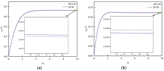
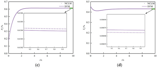
Figure 2. Response comparison under $H=0 \mathrm{km}$ and $Ma=0.2$: (a) $n_L$ responses; (b) $n_H$ responses; (c) $P_3$ responses; (d) $T_5$ responses.

As we can see from Figure 2, our proposed approach displayed outstanding performance in modeling aero-engine SVMs. The steady-state errors of SVM and NCLM were within $\pm \left(1\times {10}^{-4}\right)\%$, indicating the high modeling accuracy and efficiency of our methodology.

5.1.2. Flight Envelope Division

In accordance with the procedure outlined in Section 3.2, we divided the flight envelope using the AP clustering algorithm based on the gap measure of the linear model between the working points. For the AP clustering algorithm, we set the damping coefficient $\lambda$ to 0.5, the stable cluster center condition parameter $t_{\mathrm{conv}}$ to 50, and the maximum number of iterations $t_{\max }$ to 500. The bias parameter $p$ is responsible for determining the number of clustering centers, and a larger bias parameter results in a smaller number of clustering centers. In this paper, we set the bias parameter to twice the median of the similarity matrix to balance the trade-off between modeling accuracy and model complexity.

After iterative computation, the flight envelope, depicted in Figure 1, was divided into 10 classes, as shown in Figure 3, with the clustering centers listed in Table 3.

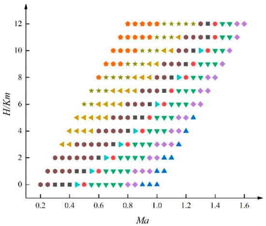
Figure 3. Flight envelope clustering results using gap metric.

Table 3. Cluster center locations.

Number	$\mathit{M}\mathit{a}$	$\mathit{H}$/$\mathbf{Km}$	Number	$\mathit{M}\mathit{a}$	$\mathit{H}$/$\mathbf{Km}$
1	0.7	3	6	0.95	7
2	0.7	6	7	1.0	4
3	0.8	3	8	1.0	6
4	0.85	9	9	1.15	3
5	0.9	11	10	1.20	5

The aforementioned clustering center serves as the nominal point for the T-S fuzzy model. After evaluating the SVMs at the nominal points, we derived ten fuzzy rules for the T-S fuzzy model, with the $1^{st}$ and ${10}^{th}$ rules illustrated below:

$$\begin{array}{l}{\mathrm{R}}^1:\mathrm{if}H=3\mathrm{km}\mathrm{and}Ma=0.7,\mathrm{then}\\ A=\left[\begin{array}{cc}-1.2171& 1.0220\\ -0.2198& -1.1797\end{array}\right],B=\left[\begin{array}{cc}0.3219& 0.5174\\ 0.3295& 0.2978\end{array}\right],C=\left[\begin{array}{cc}1& 0\\ 0& 1\\ 0.4390& 1.4342\\ 0.1129& -0.5674\end{array}\right],D=\left[\begin{array}{cc}0& 0\\ 0& 0\\ 0.1703& -0.6777\\ 0.4562& 0.0896\end{array}\right].\end{array}$$

$$\begin{array}{l}{\mathrm{R}}^{10}:\mathrm{if}H=5\mathrm{km}\mathrm{and}Ma=1.2,\mathrm{then}\\ A=\left[\begin{array}{cc}-2.6999& 1.0564\\ -0.4978& -1.3340\end{array}\right],B=\left[\begin{array}{cc}0.3818& 0.3818\\ 0.3454& 0.3269\end{array}\right],C=\left[\begin{array}{cc}1& 0\\ 0& 1\\ 1.2487& 1.4562\\ -0.1812& -0.5273\end{array}\right],D=\left[\begin{array}{cc}0& 0\\ 0& 0\\ 0.1622& -0.6831\\ 0.4446& 0.1081\end{array}\right].\end{array}$$

We regret that due to space limitations, we cannot provide the remaining rules in detail.

5.1.3. Fuzzy Membership Solving

Following the process outlined in Section 3.3, we generated the membership matrix as follows:

$$F={\left[\begin{array}{cccccccccc}0.4108& 0.0913& 0& 0& 0& 0.4979& 0& 0& 0& 0\\ 0.5739& 0& 0& 0& 0& 0.4261& 0& 0& 0& 0\\ ⋮& ⋮& ⋮& ⋮& ⋮& ⋮& ⋮& ⋮& ⋮& ⋮\end{array}\right]}_{221\times 10}$$

By utilizing the aforementioned membership matrix and the two-dimensional nearest neighbor interpolation method, it is possible to calculate the value of the membership function for a particular flight condition, enabling the derivation of the T-S fuzzy model at that point.

In the subsequent part of this section, we validate the accuracy of the developed T-S fuzzy model consisting of 10 fuzzy rules.

First, we validate the accuracy of the developed model on the training sample set, which comprises 221 steady-state points given in Figure 1. For validation, we choose the working point where $H=10 \mathrm{km}$ and $Ma=1.2$. As in Section 5.1.1, we compare the output responses of the T-S fuzzy model and NCLM using the same inputs. Due to space limitations, we present only the response comparison results for the 1% $W_f$ step input, as shown in Figure 4.

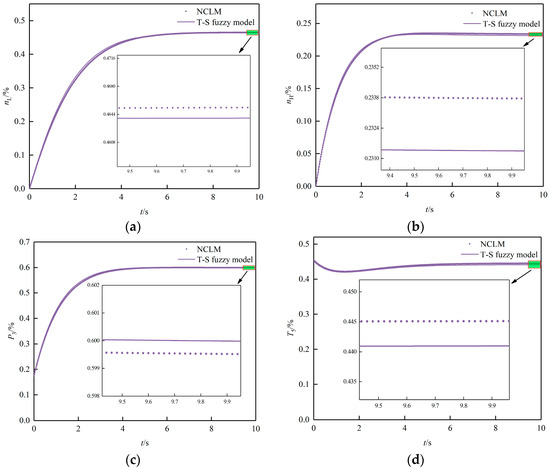
Figure 4. Response comparison under $H=10 \mathrm{km}$ and $Ma=1.2$: (a) $n_L$ responses; (b) $n_H$ responses; (c) $P_3$ responses; (d) $T_5$ responses.

As shown in Figure 4, the T-S fuzzy model outputs closely matched those of the NCLM, with steady-state errors between the two models being within $\pm \left(5\times {10}^{-3}\right)\%$. Obviously, the modeling error of the T-S fuzzy model is higher than that of the SVM. This can be attributed to the fact that the T-S fuzzy model is constructed based on the secondary modeling of the SVM, which inevitably generates additional errors.

Next, to validate the generalization capability of the developed model across the flight envelope, we conducted simulations at non-identified working points within it. Specifically, in addition to the 221 points previously used for model training, we randomly selected 10 points within the flight envelope for model accuracy verification. Due to space limitations, precise information about these operating points cannot be provided. Using the same simulation conditions as in Figure 4, we obtained the root mean square error (RMSE), denoted as $E_{\mathrm{rms}}$, between the output response of the T-S fuzzy model and NCLM at these working points for the same input. Figure 5 displays the RMSE at each simulation point.

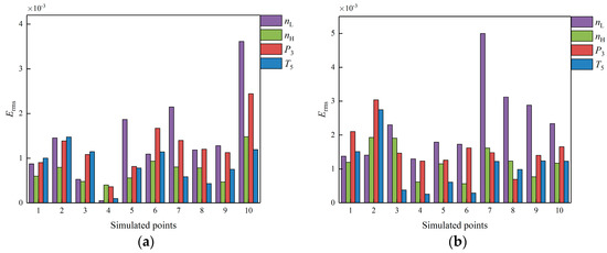
Figure 5. $E_{\mathrm{rms}}$ at different working points: (a) for 1% $W_f$ step input; (b) for 1% $A_8$ step input.

As illustrated in Figure 5, the RMSE of the T-S fuzzy model at non-identified working points was on the order of ${10}^{-3}$, which indicates that the T-S fuzzy model had good generalization ability. Although there is some error in the model, it is sufficient to meet the accuracy requirements of the controller design, which are verified in Section 5.2.

5.2. Controlled System Simulation

To further illustrate the effectiveness of the method proposed in this paper, simulation cases are given in this section to verify whether the established T-S fuzzy model is capable of replacing the original model for controller design.

Combined with the actual working of the aero-engine, we set the sampling period as $h=0.02 \mathrm{s}$, the delay upper bound as ${\tau }_M=0.1 \mathrm{s}$, the $H\infty$ performance level as $\gamma =2.4$, tuning parameter as $\rho =0.17$. By solving the LMIs of Theorem 1, the controller parameters can be obtained as follows:

$$K_1=\left[\begin{array}{cc}-1.4905& -2.0884\\ -0.3179& 0.0894\end{array}\right] K_{10}=\left[\begin{array}{cc}-0.7637& -1.7181\\ -0.0696& 0.1685\end{array}\right]$$

where $K_1$ and $K_{10}$ are the controller gains corresponding to the 1st and 10th rules, respectively. Due to space limitations, details of the remaining parameters are not provided.

We then choose the working point $H=3.9\mathrm{km}$, $Ma=1.15$ to evaluate the effectiveness of the controller designed using the T-S fuzzy model proposed in this paper. Assume that $n_L$ and $n_H$ have initial deviations of 1% and −1%, respectively, i.e., $x\left(0\right)={\left[\begin{array}{cc}1& -1\end{array}\right]}^T$. Additionally, we set the external perturbation $w\left(t\right)=x^T\left(t\right)N\zeta \left(t\right)$, where $\zeta \left(t\right)\in {ℝ}^2$ is Gaussian white noise with a zero mean and a noise intensity of $N=diag\left\{0.5,0.5\right\}$.

To assess the effectiveness of the T-S fuzzy model-based controller proposed in this paper, a comparison controller was introduced using the gain scheduling approach based on flight envelope division [24]. The design process of the comparison controller was as follows. The flight envelope was divided into nine subregions based on the generalized Euclidean distance, and the midpoint of each subregion was selected as its nominal point, as shown in Figure 6. Then, the corresponding controller was designed for each subregion and combined to obtain the gain scheduling controller for the full flight envelope. In actual operation, the controller corresponding to the flight conditions of the engine was selected according to the $H$ and $Ma$ of the engine.

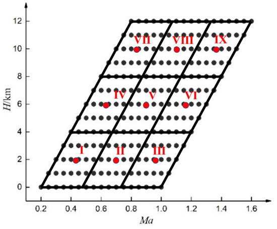
Figure 6. Flight envelope clustering results using generalized Euclidean distance metric.

Noting that the selected operating point is in subregion III, the controller parameters for the gain scheduling approach were obtained by solving LMI (19) in conjunction with the model of the nominal point in this region, as follows:

$$K_{\mathrm{sch}}=\left[\begin{array}{cc}-0.1301& -1.4793\\ 1.4625& 1.1370\end{array}\right]$$

Figure 7 depicts the system responses under the influence of both controllers. It is observed that both controllers can converge the system states far from the equilibrium point to the equilibrium point. However, it is apparent that the convergence rate of the system under the action of the proposed controller in this paper is significantly better than that of the comparison controller, and the overshoot is relatively small. The reason for this phenomenon lies in the difference in the design methods of the two controllers, specifically as follows. (1) Flight envelope division—our approach uses the gap metric between linear models, while the comparison method uses the generalized Euclidean distance metric, which is coarser in comparison. (2) Controller calculation—the T-S fuzzy controller in our approach is obtained by combining the models of all nominal points and membership values. In contrast, the comparison method uses corresponding nominal point controllers directly, which results in less information used and less accuracy in control.

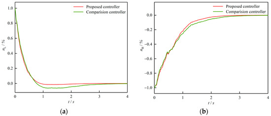
Figure 7. System responses under two different controllers: (a) $n_L$ responses; (b) $n_H$ responses.

After comparing the design process and the control effects of the two methods, it could be concluded that the gain scheduling controller is simpler to design compared to the fuzzy controller and easy to understand and implement. However, it has certain limitations in terms of control accuracy and robustness. In contrast, although the design process of the T-S fuzzy controller is more complex, it offers equally simple implementation and higher control accuracy.

To further validate the efficacy of the model and the proposed control method under varying external perturbations caused by environmental effects and noise during actual operation of the aero-engine, the following cases within the selected flight envelope were selected for further verification.

Condition 1: $H=3.9 \mathrm{km},Ma=1.1,N_1=diag\left\{1.5,1.5\right\}$;

Condition 2: $H=8.5 \mathrm{km},Ma=1.4,N_2=diag\left\{0.5,0.5\right\}$;

Condition 3: $H=10 \mathrm{km},Ma=1.5,N_3=diag\left\{1.5,1.5\right\}$.

Figure 8 shows the system’s state responses under different conditions while keeping each parameter setting constant. It is observed that the controller developed based on the T-S fuzzy model can guarantee the asymptotic convergence of the system under various disturbance conditions and working points. This further highlights the effectiveness of the model and control method proposed in this paper.

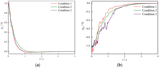
Figure 8. System responses under three different working conditions: (a) $n_L$ responses; (b) $n_H$ responses.

6. Conclusions

This paper presents a novel approach to model an aero-engine using the multi-strategy improved L-SHADE algorithm to establish a high-precision SVM, the AP clustering algorithm to divide the flight envelope, and the SVM as the subsequent part of the T-S fuzzy model to obtain the T-S fuzzy model of the aero-engine within the full flight envelope. The proposed T-S fuzzy control method based on distributed control architecture is then used to design the controller. The simulation results indicate that the proposed modeling method achieves high accuracy and meets the requirements of controller design accuracy. Furthermore, the proposed method outperforms the gain scheduling method based on flight envelope division in achieving a better control effect. This study contributes to the development of advanced control strategies for aero-engines and highlights the potential of the T-S fuzzy model for solving similar engineering applications. Future research could focus on improving the robustness and effectiveness of the proposed control method for possible real-world implementation.

References

- Zhou, B.; Xie, S.; Wang, F.; Hui, J. Multi-step predictive compensated intelligent control for aero-engine wireless networked system with random scheduling. J. Frankl. Inst. 2020, 357, 6154–6174. [Google Scholar] [CrossRef]
- Zhang, L.; Xie, S.; Yu, Z.; Ren, L.; Zhou, B.; Wang, H.; Peng, J.; Wang, L.; Li, Y. Aero-engine DCS fault-tolerant control with Markov time delay based on augmented adaptive sliding mode observer. Asian J. Control 2018, 22, 788–802. [Google Scholar] [CrossRef]
- Wang, W.; Xie, S.; Peng, J.; Zhang, Y.; Wang, H.; Zhou, B.; Wang, L. Dual-terminal event-triggered dynamic output feedback H∞ control for aero engine networked control systems with quantization. Int. J. Robust Nonlinear Control 2023, 33, 697–719. [Google Scholar] [CrossRef]
- Sugiyama, N. Derivation of system matrices from nonlinear dynamic simulation of jet engines. J. Guid. Control Dyn. 1994, 17, 1320–1326. [Google Scholar] [CrossRef]
- Lin, Y.H.; Zhang, H.B. Establishment of State Variable Model of Aeroengine with Improved Least Square Fitting. Appl. Mech. Mater. 2010, 40–41, 27–33. [Google Scholar]
- Wang, B.; Shi, Y.; Wang, X. Aeroengine State Variable Modeling based on the PSO Algorithm. In Proceedings of the IEEE 2013 Chinese Automation Congress, Changsha, China, 7–8 November 2013; pp. 177–180. [Google Scholar]
- Lu, F.; Qian, J.; Huang, J.; Qiu, X. In-flight adaptive modeling using polynomial LPV approach for turbofan engine dynamic behavior. Aerosp. Sci. Technol. 2017, 64, 223–236. [Google Scholar] [CrossRef]
- Sugeno, T.T.a.M. Fuzzy identification of systems and its applications to modeling and control. IEEE Trans. Syst. Man Cybern. 1985, 15, 116–132. [Google Scholar] [CrossRef]
- Zhou, B.; Xie, S.; Hui, J. H-infinity control for T-S aero-engine wireless networked system with scheduling. IEEE Access 2019, 7, 115662–115672. [Google Scholar] [CrossRef]
- Li, R.; Guo, Y.; Nguang, S.K.; Chen, Y. Takagi-Sugeno fuzzy model identification for turbofan aero-engines with guaranteed stability. Chin. J. Aeronaut. 2018, 31, 1206–1214. [Google Scholar] [CrossRef]
- Cai, K.; Xie, S.; Wu, Y. Identification of aero-engines model based on T-S fuzzy model. J. Propuls. Technol. 2007, 28, 194–198. [Google Scholar]
- Wang, L.; Xie, S.; Miao, Z.; Ren, L.; Zhang, Z. Identification of T-S fuzzy model for aero-engine based on flight envelop division. J. Aerosp. Power 2013, 28, 1159–1165. [Google Scholar]
- Xu, Y.; Pan, M.; Huang, J. Fuzzy modeling and robust control based on intelligent feature extraction method. J. Aerosp. Power 2021, 36, 1545–1555. [Google Scholar]
- Zames, G.; El-Sakkary, A.K. Unstable systems and feedback: The gap metric. In Proceedings of the Eighteenth Annual Allerton Conference on Communication, Control, and Computing, Urbana, IL, USA, 8–10 October 1980; pp. 380–385. [Google Scholar]
- El-Sakkary, A.K. The gap metric: Robustness of stabilization of feedback systems. IEEE Trans. Autom. Control 1985, 30, 240–247. [Google Scholar] [CrossRef]
- Jaw, L.C.; Mattingly, J. Aircraft Engine Controls: Design, System Analysis, and Health Monitoring; AIAA: Reston, NY, USA, 2009. [Google Scholar]
- Aranguren, I.; Valdivia, A.; Morales-Castañeda, B.; Oliva, D.; Abd Elaziz, M.; Perez-Cisneros, M. Improving the segmentation of magnetic resonance brain images using the LSHADE optimization algorithm. Biomed. Signal Process. Control 2021, 64, 102259. [Google Scholar] [CrossRef]
- Tanabe, R.; Fukunaga, A.S. Improving the search performance of SHADE using linear population size reduction. In Proceedings of the 2014 IEEE Congress on Evolutionary Computation, Beijing, China, 6–11 July 2014. [Google Scholar]
- Tizhoosh, H.R. Opposition-Based Learning: A New Scheme for Machine Intelligence. In Proceedings of the International Conference on International Conference on Computational Intelligence for Modelling, Control & Automation, Vienna, Austria, 28–30 November 2005. [Google Scholar]
- Frey, B.J.; Dueck, D. Clustering by passing messages between data points. Science 2007, 315, 972–976. [Google Scholar] [CrossRef] [PubMed]
- Belapurkar, R.K.; Yedavalli, R.K.; Behbahani, A. Study of model-based fault detection of distributed aircraft engine control systems with transmission delays. In Proceedings of the 47th AIAA/ASME/SAE/ASEE Joint Propulsion Conference, San Diego, CA, USA, 31 July–3 August 2011. [Google Scholar]
- Park, P.; Ko, J.W.; Jeong, C. Reciprocally convex approach to stability of systems with time-varying delays. Automatica 2011, 47, 235–238. [Google Scholar] [CrossRef]
- Qi, Y.; Tang, Y.; Ke, Z.; Liu, Y.; Xu, X.; Yuan, S. Dual-terminal decentralized event-triggered control for switched systems with cyber attacks and quantization. ISA Trans. 2021, 110, 15–27. [Google Scholar] [CrossRef] [PubMed]
- Wang, H.; Wang, D. Turbofan aero-engine full flight envelope control using H∞ loop-shaping control technique. Int. J. Adv. Mechatron. Syst. 2011, 3, 65–76. [Google Scholar] [CrossRef]
Disclaimer/Publisher’s Note: The statements, opinions and data contained in all publications are solely those of the individual author(s) and contributor(s) and not of MDPI and/or the editor(s). MDPI and/or the editor(s) disclaim responsibility for any injury to people or property resulting from any ideas, methods, instructions or products referred to in the content. |
© 2023 by the authors. Licensee MDPI, Basel, Switzerland. This article is an open access article distributed under the terms and conditions of the Creative Commons Attribution (CC BY) license (https://creativecommons.org/licenses/by/4.0/).