Article

Simulation-Based Prediction of Departure Aircraft Performance from Surveillance-like Data Using Neural Networks

ENVISA SAS, 62 Rue Montorgueil, F-75002 Paris, France
*
Author to whom correspondence should be addressed.
Aerospace 2023, 10(6), 513; https://doi.org/10.3390/aerospace10060513
Submission received: 14 April 2023 / Revised: 25 May 2023 / Accepted: 27 May 2023 / Published: 30 May 2023

Abstract

:
Estimating the environmental impact of aviation, in terms of noise and emissions, requires accurate knowledge of flight parameters such as departure/arrival procedure, aircraft mass, thrust and flap settings. However, these parameters are not available from radar/ADS-B data, which are the main sources of multiple flight-specific information including aircraft position over time. This paper introduces a novel approach to estimating these parameters from radar/ADS-B data using three neural network models trained on flight simulator data for the Boeing 747-400 airplane. The models are tested on 2204 simulated flights that are not used for training and that are transformed into radar/ADS-B data formats. The models are capable of predicting the unknown parameters for the ADS-B data format, with the weight prediction error being 2.63% of maximum takeoff weight, the average R2 score for the thrust profile prediction being 89.90% and the flap setting profile having an average R2 score of 84.68%, while for the radar-like data format, the values are 2.11%, 95.74% and 88.24%, respectively. The predicted parameters can be used to improve the environmental impact assessment of individual flights and to support policy-making and management decisions. This approach is a proof of concept based on simulation data that will need to be validated on real data before being applied in practice.

1. Introduction

Nowadays, monitoring of the environmental impact of aviation is gaining more and more attention given how critical this sector is, both at a local scale and a global scale. In order to quantify the impact in terms of noise and emissions, current mathematical models rely on supporting data that assume typical aircraft performance modeling as aircraft depart and arrive at an airport. In the case of noise, the database in use and suggested by ICAO in the document “Recommended Method for Computing Noise Contours Around Airports” [1] is the Aircraft Noise and Performance (ANP) database [2], while for engine emissions one of the publicly available sources to model the pollutant emissions is the ICAO Engine Emissions DataBank [3], which contains the emissions indices for the certified pollutants collected during the engine certification process for jet engines with a rated thrust higher than 26.7kN and assumes fixed thrust ratings for the four phases of the landing and takeoff (LTO) cycle. However, the information provided in these databases refers to very specific conditions, assuming full takeoff thrust, pre-defined thrust cut-back altitudes and flap settings, while in real operations these conditions vary according to several factors. While this approach could be a good way of representing the average impact for a fleet mix, it does not allow to take into account the impact on a flight-by-flight basis. The most accurate way to quantify the environmental impact of an aircraft would be through the use of data from real operations, that is to say to know the procedure followed by an aircraft during a departure or arrival including parameters such as the thrust, the aircraft mass and the flap used. While this information exists, through the Flight Data Recorder, it is not publicly available as it is the property of airlines. Nevertheless, data regarding the position of an aircraft during a flight can be available through the Automatic Dependent Surveillance-Broadcast (ADS-B) dataset. Similarly, data provided by the radar tower provide the same information, although the access to these data is generally not public. The main limitation of these data compared to FDR data is that they do not contain proprietary information such as aircraft mass, the thrust and the flap settings at each point, all parameters necessary to accurately estimate the environmental impact of a flight. However, these parameters could be estimated from these data with knowledge of the aircraft type and the meteorological conditions and by using physics equations. There have been some studies that have tried to estimate one or more of these unknown parameters. In [4], a method based on the aircraft total energy model is implemented that uses a reference mass for each aircraft type. Alligier and his team used the least squares method in [5] and a machine learning method in [6]. Schultz and others in [7] introduced an adaptive method to estimate the aircraft weight. J. Sun and others used the takeoff phase data in [8] for weight estimation, then in 2018 they used Bayesian inference to improve the accuracy by combining weight estimations from different flight phases [9] and later in [10] they used a recursive Bayesian method to minimize the effect of noise in the radar data. In 2020, a group of scientists used recurrent neural networks to predict the fuel flow and flap setting, based on Flight Data Recorder (FDR) data from two French airlines [11]. Their model took the last minute of data as input, to predict the next value in the time series.
In this paper, we propose a novel methodology that estimates the three unknown parameters altogether from radar/ADS-B data with an innovative approach using neural network models. The idea is to use generated radar-like data where aircraft mass, flap setting and the thrust are known and to train a model that is then able to predict the three parameters when it sees radar/ADS-B data when these are not known. As stated before, this kind of data for real flights is available from the FDR that it is generally not possible to obtain access to. To by-pass this issue, we used a flight simulator (X-Plane) to generate the data. More studies will be necessary to confirm that the neural network is trained with accurate data. The focus of this work was on departures only for one single aircraft type (Boeing 747-400).

2. Materials and Tools

In this study, the flight data for the B747-400 airliner is taken from the flight simulator X-Plane and is used to train a neural network for weight, thrust and flap setting. In order to collect a large amount of data, first the flight simulator is connected to Python using an open-source API, then an autopilot code is written for each flight phase (takeoff, climb, acceleration) and finally a code is written to generate flights using realistic noise abatement procedures specific to the aircraft type, including some variations to ensure the resulting model can generalize to a wide range of possibilities. The generated flights are then divided into two datasets, first is the training data which are used to train the neural network models, then these models are tested separately on the test dataset and when all the models are trained, the test dataset is then transformed into surveillance-like data, using the ADS-B and radar data formats to have a better assessment of the models’ performance and replicate the error they would have on real flight data.

2.1. X-Plane Flight Simulator

Although there are many options when it comes to flight simulators, X-Plane 11 was chosen because of its accuracy in simulation [12]. X-Plane uses a method called blade-element theory, which calculates these forces by breaking down the aircraft into many sections and then calculating the forces on each of them separately, to be summed up in the end over the entire aircraft body. This method is capable of providing a reliable accuracy outside of the transonic zone and is even comparable to methods far more complicated and time-consuming such as computational fluid dynamics [13].
Furthermore, X-Plane gives the user the ability to read and write data via the User Datagram Protocol (UDP) socket. Using this feature, it is possible to change the aircraft weight, control inputs, weather conditions, amount of fuel and many other variables through a third-party program including Python.
In order to communicate between X-Plane and Python, NASA’s open-source X-Plane Connect (XPC) plugin is used, which provides special functions to read and write data easily and communicate with X-Plane in real time.

2.2. Departure Procedures

In order to generate data using the flight simulator, research was carried out to understand what the typical departure procedures generally followed by aircraft are. The reference used is the ICAO Doc 9888 [14], which mentions 14 different departure procedures generally followed by Airlines, 6 of which can be used for the B747-400 aircraft chosen for this study. An example profile is shown here.
Profile 1:
  • Takeoff power and flaps, climbing at V2 plus to 243.8 m
  • At 243.8 m, set climb power
  • Constant speed climb to 457.2 m
  • At 457.2 m reduce pitch, accelerate and retract flaps on schedule
  • Constant speed climb to 914.4 m
  • At 914.4 m, accelerate to 128.6 m·s−1
  • Constant speed climb to 3048 m
During the data-generation process, the code will choose a procedure among the ones proposed in Doc 9888 for the 747-400 at random with equal distribution, then using the autopilot algorithms described later, it follows the procedure requirements with slight variations up to 3048 m altitude and then the flight is reset and the process is repeated. 12,798 flights were generated over 10 different airports to also account for different airport elevations and runway gradients.
The value of V2 mentioned here is a function of weight, weather and runway conditions and can be found in the B747-400 flight manual [15].
In what follows, first the flight simulator is introduced and then the essential methods in generating each flight are explained in detail.

2.3. ADS-B and Radar Data

When it comes to tracking flight data, there are two main technologies that are widely used: Automatic Dependent Surveillance-Broadcast (ADS-B) and radar.
Radar systems use radio waves to track an airplane’s position and velocity by sending a signal which then bounces back to the radar. The time intervals between data points depends on the period of rotation of the radar, which is usually around 4 s [16]. ADS-B, however, uses GPS to determine the altitude, position and velocity of the aircraft with respect to ground stations and other aircraft in the area using radio waves, and the time interval between data points may vary depending on the source and according to [17] which is used for acquiring the data the time intervals for a flight are in a wide range of 6 to around 60 s. As these two are the main sources of collecting flight data, in this article a method is introduced to replicate these data formats, using the X-Plane’s output data for each flight, to then be used for a more realistic testing of the models.
In this paper, two months of flights (January and July 2019) for the airports of Amsterdam Schiphol (AMS) and Paris Charles de Gaulle (CDG) purchased from FlightRadar24 [17] are used for comparison purposes.

3. Flight Generation

In order to generate flights with enough variety, each variable of the chosen profile is randomized, using arbitrarily chosen randomness for each variable, so that even two flights with the same weight and profile will look slightly different. This added variation to the variables serves to emulate the human factors and gives the models enough variety to ensure generalization. To be more precise, 2% variation is added to the end altitudes, 5% to the end calibrated airspeed values and the amount of climb angle reduction during the acceleration phase will have 20% variation. The reason for the disparity in these values is the order of importance of each variable; for example, it is important for the indicated airspeed not to exceed 128.6 m·s−1 below 3048 m above mean sea level, because this is part of the Standardized European Rules of the Air [1414]. The acceleration start altitude is also mentioned strictly in the departure procedures present in [14] and the only value that can be changed more freely is the climb angle reduction during the acceleration phase, since according to the noise abatement procedures mentioned before, there is no specific climb angle or climb rate to follow during acceleration.
After the randomization of the chosen profile, weather conditions are also given some variance through sea level temperature and pressure, wind speed and direction and the runway condition. For the current study, the sea level temperature is chosen randomly for every flight from a range of −5 °C to 30 °C and the sea level pressure is similarly chosen from a range of 0.97 atm to 1.03 atm.
In the X-Plane environment, it is also possible to set up to three layers of wind, each characterized by a specific velocity, direction and shear which determines the velocity change over time. For example, if the first layer is set up to 15.43 m·s−1 speed at 1000 m altitude above ground, then X-Plane automatically produces a wind velocity profile from 1000 m to the ground level, in a way that velocity increases with altitude. Second and third layers can also be given and X-Plane will interpolate the wind characteristics between layers. For this study, the wind speed is chosen with even distribution between 0 and 23.15 m·s−1 at 4000 m altitude. However, since the takeoff runway in reality is chosen in a way to reduce the crosswind affecting the aircraft [18], the wind direction during the data generation has a non-even distribution based on the runway direction. To be more specific, the wind direction is chosen from a list of numbers with the mean value equal to the runway heading, within the range of the runway heading plus and minus 45 degrees. For the Amsterdam airport runway, 36R is an example which has a heading of about 3 degrees taken from X-Plane; this method will yield the wind direction distribution shown in Figure 1.
The runway condition in X-Plane can be chosen between three options of dry, damp and wet and these control the runway friction factor. For this study, the runway condition is chosen to be dry with 50% probability, damp with 25% probability and wet with also 25% probability.
Finally the weight of the aircraft is set randomly with an even distribution in a range of 236,000 kg to 397,000 kg. This range according to [19] seems to be an appropriate weight range for the B747-400 to be closely related to real flights. To set the desired weight for the aircraft in X-Plane after resetting each flight, the payload weight is changed accordingly.

3.1. Takeoff

After the weight is chosen, the takeoff function will start by setting up the flap, then knowing the flap setting, the takeoff velocities, V2 and rotation velocity are determined according to [15] with slight variation added to increase the randomness of the flights. The most common flap settings for B747-400 takeoff are flaps 10 and 20 [19], so one of these was chosen randomly at the start of each takeoff.

3.1.1. Reduced Takeoff Thrust

Most of the time in real flights, in order to save fuel and reduce emissions, as well as increase the engine lifetime, pilots use a reduced thrust as opposed to max takeoff thrust [20] and they obtain the appropriate amount of thrust reduction from a built-in application made by the airline not available to the public [21] which uses a variety of parameters such as weather conditions, runway conditions and weight. In order to replicate this in X-Plane to some degree, for each flight a random reduction of thrust is considered which is in the range of 0 to 35% of the aircraft maximum takeoff thrust. According to [20], the takeoff thrust has to be more than 75% of the maximum thrust, but for this study lower thrust values are also considered for two main reasons, first to increase the variation of the flights and for the final model to be able to better generalize the relationship between different parameters and the thrust, and secondly because a nominal value is chosen for the maximum thrust and this can be lower due to the specific weather conditions for each flight.

3.1.2. Throttle Controller

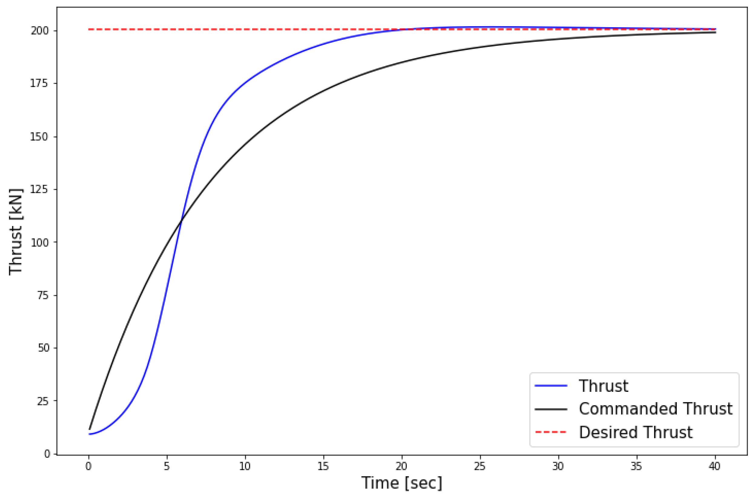
After the desired thrust value is set, this controller will try to achieve the commanded thrust. To this aim, a PID controller is designed which receives a filtered thrust command as input and then calculates the proper throttle handle position as follows.
T h r u s t c [ k ] = T h r u s t d d t T + 1 d t T T h r u s t c [ k 1 ] T h r u s t e [ k ] = T h r u s t c [ k ] T h r u s t [ k ] T h r u s t c [ k ] T h r o t t l e [ k ] = T h r o t t l e [ k 1 ] + k p T h r u s t e [ k ] + k d T h r u s t e [ k ] T h r u s t e [ k 1 ] d t + k i T h r u s t e d t T = 8 [ s e c ] k p = 0.02 k d = 0.015 k i = 0.0022
In the above equations, T h r u s t c is the command thrust, T h r u s t d is the desired thrust calculated from the reduced takeoff thrust section, T is the thrust command filter time constant, d t is the time step and [ k ] shows the k-th time step during the simulation. The controller parameters are of course chosen in a way for the actual thrust to follow closely the commanded thrust and this is achieved via trial and error. Figure 2 shows the thrust controller performance. Using this controller, after about 20 s from the start of takeoff, the thrust will reach the desired value.

3.1.3. Rudder Control

Since the aircraft might be facing strong cross winds during takeoff, a good rudder controller is needed to keep the aircraft heading straight on the runway. For this purpose, a PID controller is designed as follows.
ψ e = ψ d ψ R u d d e r = k p ψ e + k d d ( ψ e ) d t + k i ψ e d t k p = 0.8 k d = 0.6 k i = 0.2
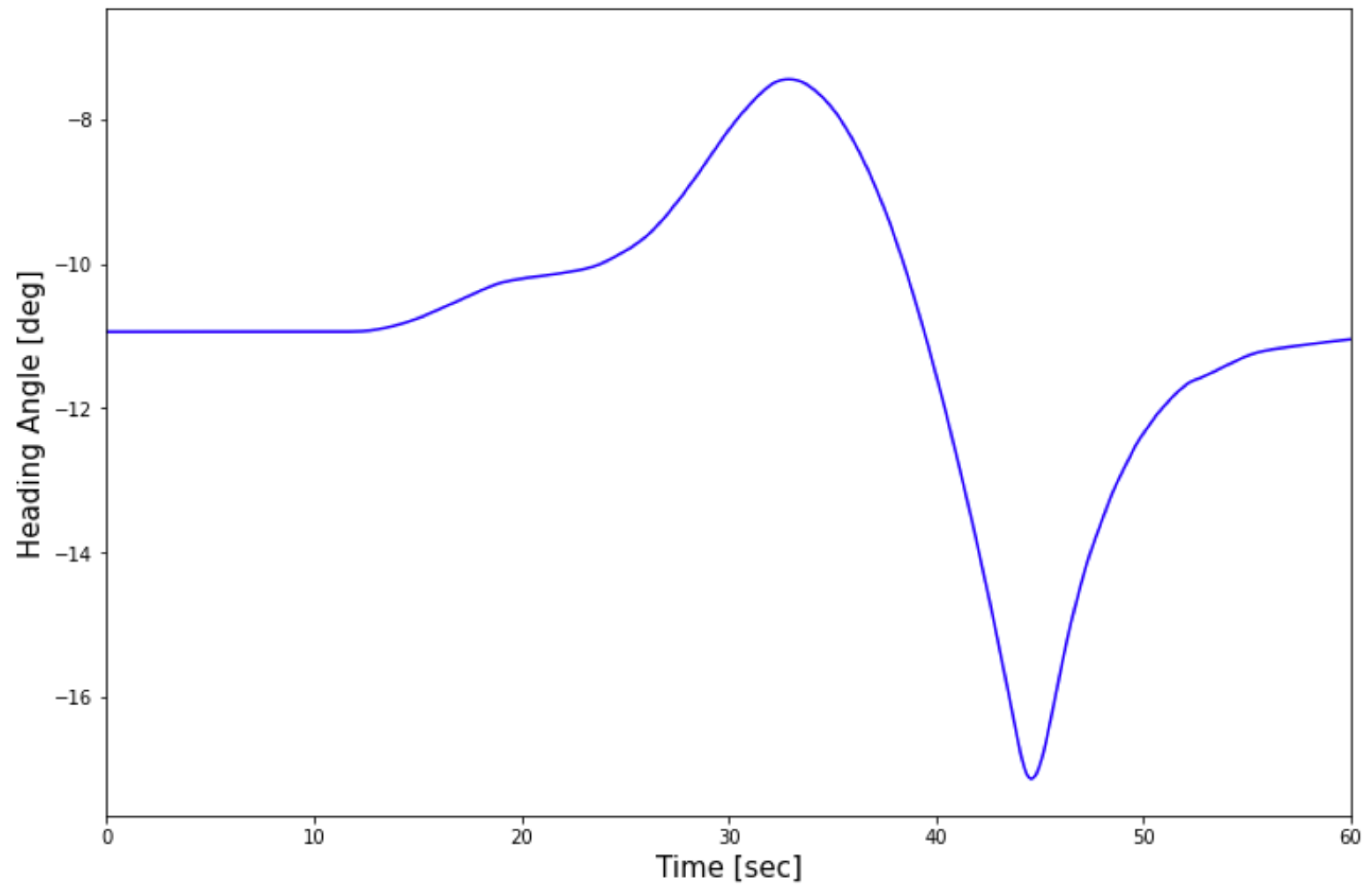
In this equation, ψ represents the true heading of the airplane and subscripts c, d and e denote the command, desired and error values, respectively. Testing the controller performance for the heaviest case of 397,000 kg takeoff weight, the fastest wind speed on the ground equal to 16.5 m·s−1 and facing a very strong crosswind by putting the wind direction at 45 degrees with respect to the runway heading, the result of heading control is as shown below. As is seen in Figure 3, even in the harshest weather conditions the controller manages to keep the aircraft on the correct path.

3.2. First Climb

The climb function in the code has the primary objective of controling the climb angle in a way to keep the calibrated airspeed constant, which is the same approach as real flights. The flap setting in this segment is the same as takeoff.

3.2.1. Elevator Control

The elevator control surface is used to control the climb angle. In order to calculate an appropriate elevator deflection, an estimate of the amount of climb angle error is needed and to this aim, first assuming the goal is to keep the ground speed constant, the following approximate equations can be written.
T c o s ( α ) D m g s i n ( γ ) = m a T c o s ( α ) D m g s i n ( γ + Δ γ ) = 0
In the above equation, T is the total thrust, a is the rate of change for the ground speed with respect to time, α is the angle between the thrust vector and the flight path, g is the constant of gravity, m is the aircraft mass, D is the aerodynamic drag and γ is the climb angle. The goal here is to find the value for the change of climb angle Δ γ which is needed for the ground speed to remain constant. Subtracting the two equations, the following is reached:
g s i n ( γ ) + a g s i n ( γ + Δ γ ) = 0 g s i n ( γ ) + a g s i n ( γ ) c o s ( Δ γ ) g c o s ( γ ) s i n ( Δ γ ) = 0
Since the value of Δ γ is small, it can be assumed that c o s ( Δ γ ) = 0 and s i n ( Δ γ ) = Δ γ and the value of Δ γ can be estimated as follows:
Δ γ = a g c o s ( γ )
So, when the ground speed is increasing, an increase in climb angle is needed to keep the ground speed constant and when the ground speed is decreasing, a decrease in climb angle is needed for the same effect. However, the goal of the climb function is to keep the calibrated air speed constant, but since the controller only needs an approximation of the climb angle change, the above equation can be used by changing the value of a, to make it the rate of change of the calibrated air speed, so the same as before, when the calibrated air speed is increasing the controller will try to decrease the climb angle to keep it constant.
Having an estimate of the desired climb angle at every time step, using a PID controller can yield the appropriate elevator deflection.
γ d [ k ] = γ [ k ] + Δ γ [ k ] γ c [ k ] = γ d [ k ] d t T γ + γ c [ k 1 ] 1 d t T γ γ e k = γ c [ k ] γ [ k ] E l e v a t o r [ k ] = k p γ e [ k ] + k d γ e [ k ] γ e [ k 1 ] d t + k i γ e d t T γ = 10 [ s e c ] k p = 0.11 k d = 0.05 k i = 0.01
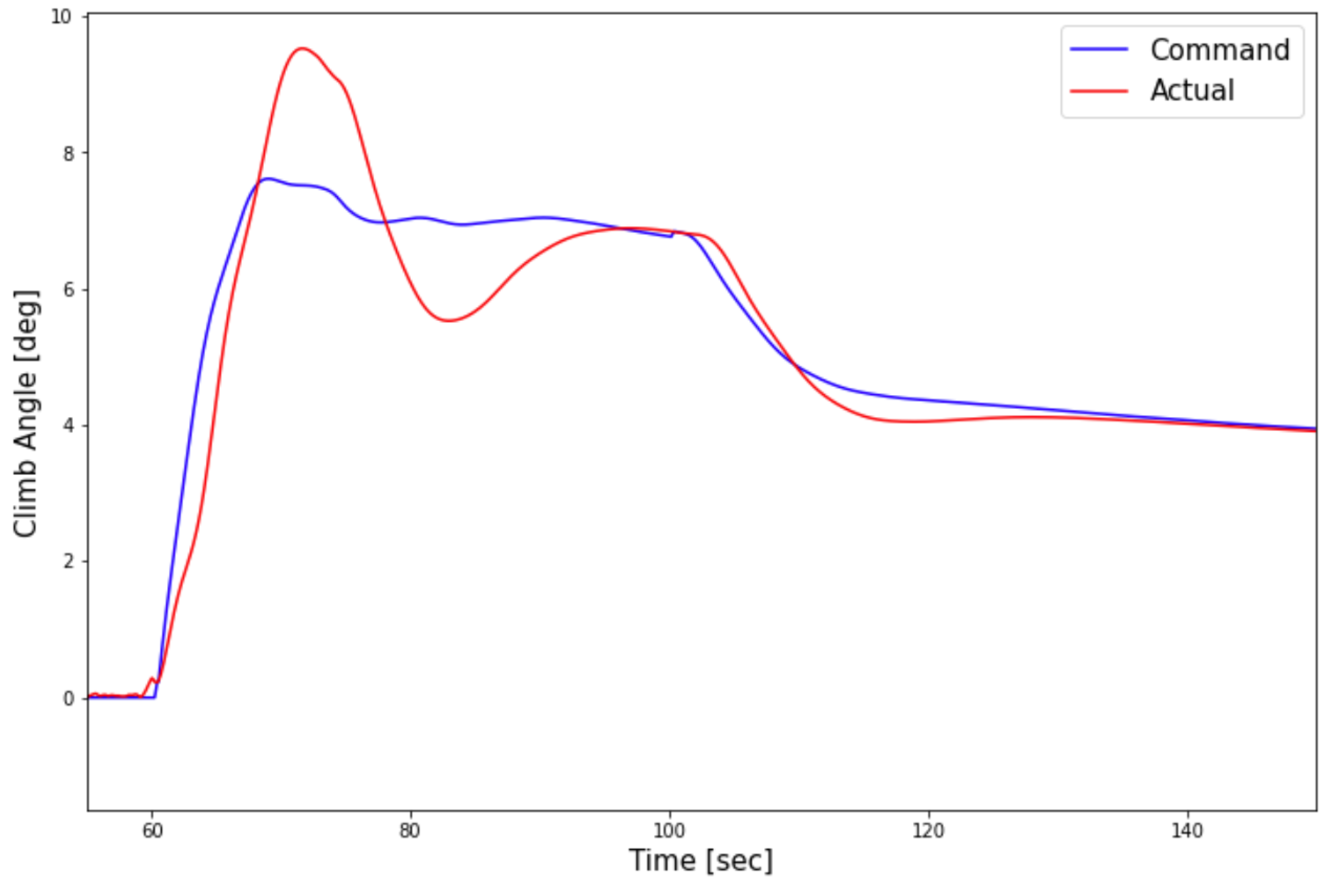
In these equations, γ d , γ c and γ e are the desired, commanded and error climb angle values, respectively, and T γ is the time constant for the filter applied. The filter that is being introduced here keeps the system from becoming unstable, since there exists an inherent delay of response in the output. To be more precise, after a change in the elevator command, first the aircraft pitch angle will change, which will result in a change in lift, which in turn will change the climb angle. The high time constant here is chosen because during the first climb the speed is quite low and the climb angle starts to increase from zero and these factors can cause the plane to crash if the filter is chosen to be too fast. Figure 4 shows the performance of the climb angle controller.
As can be seen, the controller is able to follow the commanded climb angle closely with reasonable response time and overshoot. The controller was designed to have high settling time to be more in line with real flights and not to have fast changes in the climb angle. Note that the controller is only designed to replicate real flights and the viability of the controller based on inputs is of no concern here.

3.2.2. Banking

For the climb segments, a random bank angle is chosen with a normal distribution around zero with 6.5 degrees standard deviation. The banking duration is chosen randomly from the range of 30 to 60 s with even distribution so there can be enough steady state data during banking for the model. For this purpose, another PID controller is designed which takes the bank angle error and calculates the appropriate aileron deflection command.
ϕ e = ϕ d ϕ A i l e r o n = k p ϕ e + k d d ( ϕ e ) d t + k i ϕ e d t k p = 0.1 k d = 0.15 k i = 0.007
Performance of this controller is tested by giving a command bank angle of 30 degrees and the result is shown below.
As can be seen in Figure 5, after about 20 s the controller stabilizes the airplane on the desired bank angle and after the bank duration ends it will revert back to the zero bank angle smoothly. It is worth mentioning that due to the Easy Access Rules for Standardised European Rules of the Air [1414], it is forbidden to bank more than 15 degrees below 122 m altitude and this rule has been considered in the code, for the flights to be as close as possible to their real counterpart.

3.3. Acceleration

In this segment, the airplane starts to lower the climb angle in order to accelerate. To achieve this, the desired climb angle calculated in the previous segment will be reduced by a certain percentage chosen randomly from a range of 45 to 75 percent. This segment is where most of the randomness in the generated flights comes from and the reason is that there are no specific rules to follow except the maximum allowed calibrated airspeed before 3048 m which is 128.6 m·s−1.

3.3.1. Elevator Control

In this segment, the desired climb angle is passed through a filter to obtain the command climb angle and then by using another PID controller the appropriate elevator command is calculated as follows.
γ c [ k ] = γ d [ k ] d t T γ + γ c [ k 1 ] 1 d t T γ E l e v a t o r [ k ] = k p γ e [ k ] + k d γ e [ k ] γ e [ k 1 ] d t + k i γ e d t T γ = 5 [ s e c ] k p = 0.15 k d = 0.12 k i = 0.08
Since the acceleration part is much shorter than the first climb segment, the time constant of the filter is chosen to be faster than the previous segment. The performance of this controller can be seen in Figure 4, where after the climb segment the commanded climb angle is reduced and it can be seen that the actual climb angle converges to the command after about 30 s which is much faster than the climb segment controller.

3.3.2. Flap Retraction

The flaps will be retracted on a specific schedule and this is where the V 2 parameter taken from the flight manual [15] is useful. Based on this value, upon reaching the speed limit for a certain flap setting, it will be reduced to the next flap handle position. The flap is communicated to X-Plane through a designated scalar value for each flap setting which is taken from X-Plane and is a value between 0 and 1, also shown in Table 1.
According to this table, whenever the plane reaches the speed of V 2 + 10.2 m·s−1, then the flaps will be retracted to 5 and then after each 10.2 m·s−1 acceleration, the flaps will be retracted further until they are fully up.

3.3.3. Throttle Setting

If in this segment a thrust reduction is requested by the noise abatement procedure, then the throttle will be randomly reduced by between 4 and 11 percent; otherwise, the throttle will remain constant in this segment.

3.4. Second Climb

Any climb segment that comes after an acceleration phase, will have a different function than the first climb, because the change in speed requires a different set of parameters in the controller. The banking and the climb angle controller algorithms are the same as the first climb segment and only the controller parameter values are changed. The main difference here is that after 5 s has passed from the start of this segment, the throttle controller will adjust the throttle in a way that the engine power remains constant over time. The following PID controller is used to achieve this.
P o w e r e [ k ] = P o w e r d [ k ] P o w e r [ k ] T h r o t t l e [ k ] = T h r o t t l e [ k 1 ] + k p P o w e r e [ k ] + k d P o w e r e [ k ] P o w e r e [ k 1 ] d t + k i P o w e r e d t k p = 0.02 k d = 0.015 k i = 0.0022
It is worth noting that since the error in this algorithm is a percentage of the desired value, the controller parameter values here are the same as the ones used during takeoff. The difference here is that since the change in thrust is gradual, there is no need for a filter to be applied.

3.5. Generated Flights

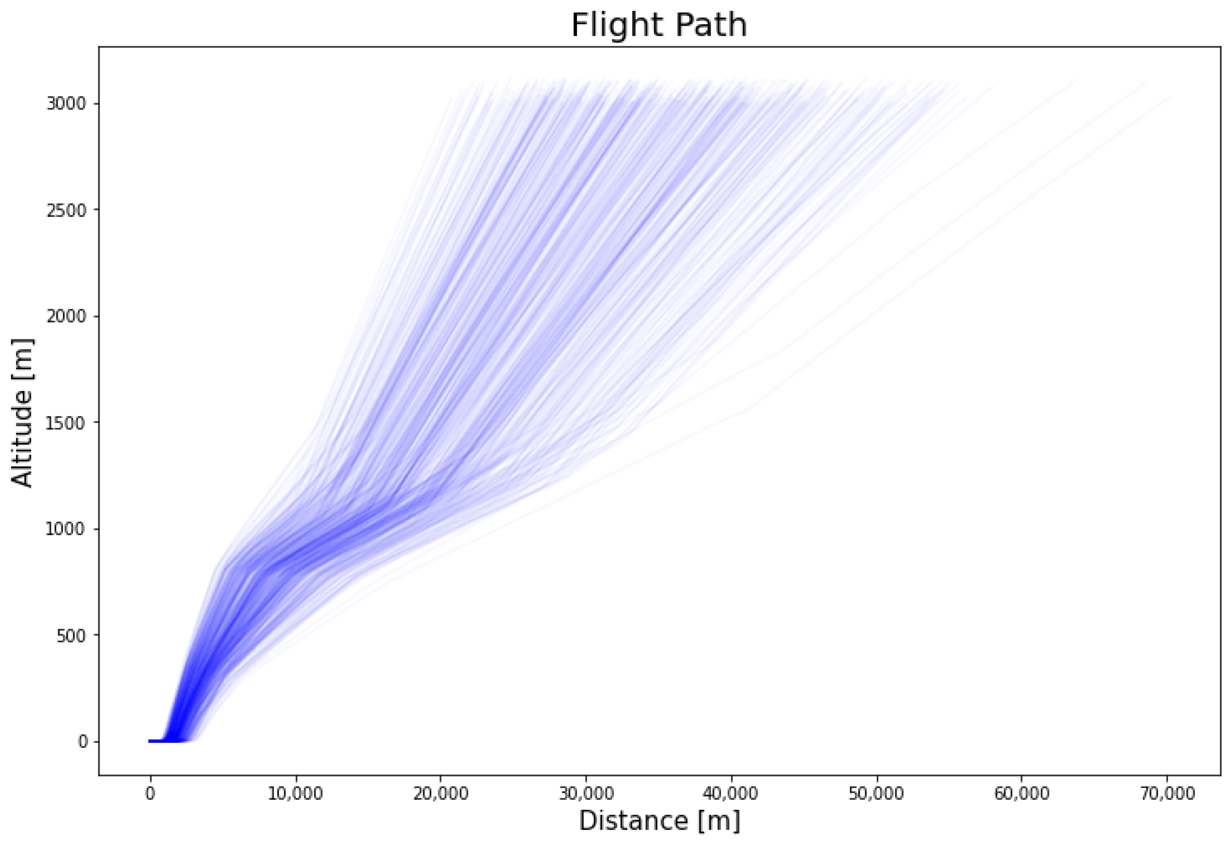
The flight process from takeoff, up to 3048 m altitude above ground level is repeated from 10 airports and 12,798 flights are generated overall. As an example, the flight paths of 500 flights generated in the AMS airport are shown in the Figure 6.
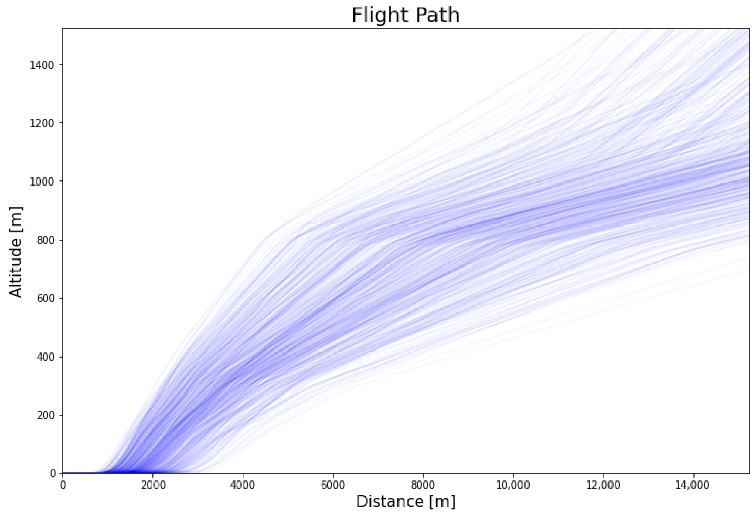
To illustrate more clearly the difference in flight paths in the beginning, the following figure shows the flights up to 1524 m above ground and presented in Figure 7.
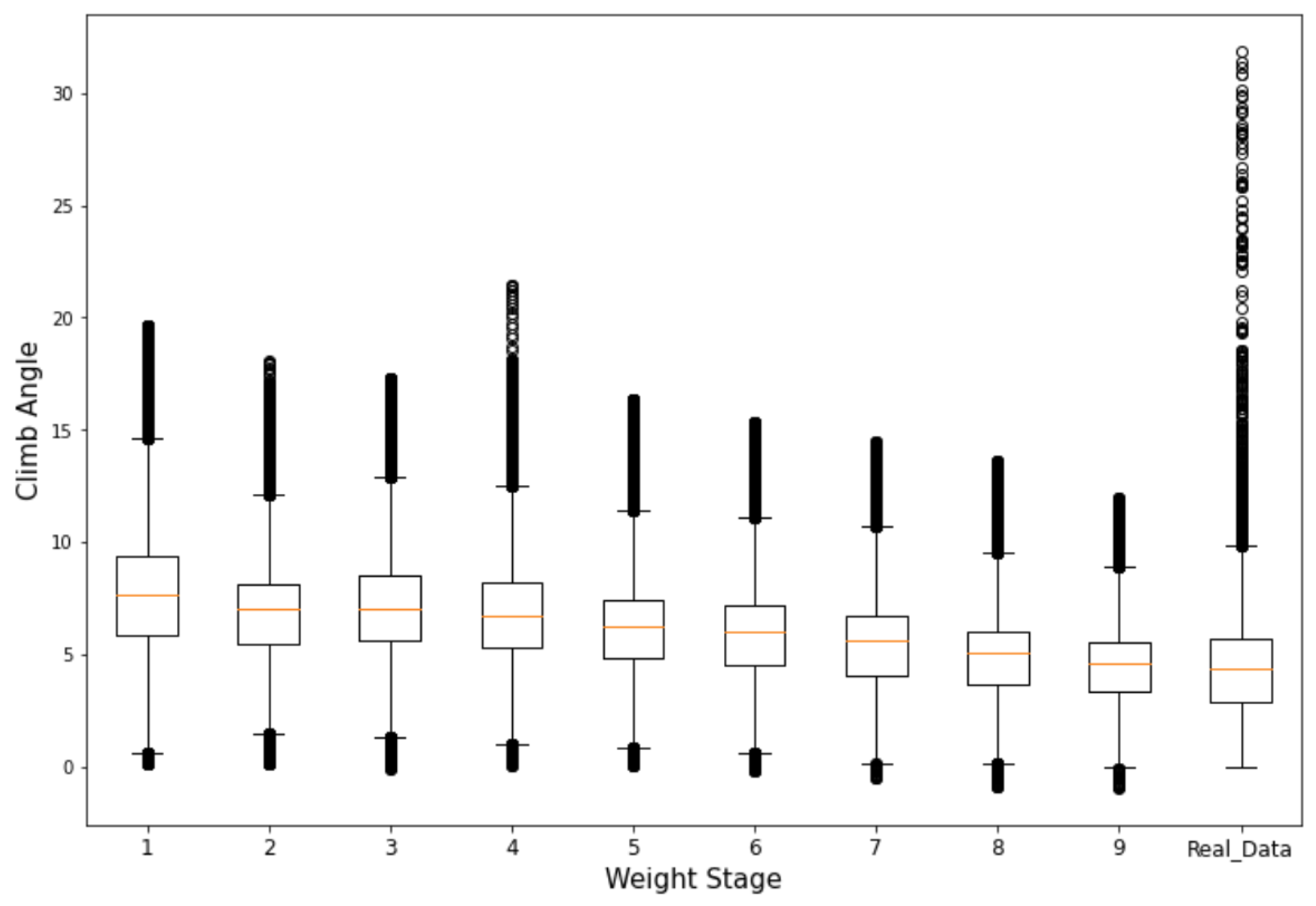
To ensure that the results are close to reality, and that there is good variety in the flights, a simple check is undertaken with the distribution of climb angles taken from the ADS-B data for the B747 flights from Amsterdam Schiphol airport [17], shown in Figure 8. In this figure, the higher stages have higher weights and as can be seen the distribution of the real flight climb angle is closer to the heavier weight stages of the generated flights. This of course is expected as most of the commercial flights are in the heavier range [19]. Overall, the data generation covers a significant variety in the flights while maintaining a similarity to real flights, which will be beneficial not only for the model to better generalize, but also for the model to be used on real flight data.

4. Neural Network Models

Using the collected data, three different neural network models with the architecture of multilayered perceptrons (MLP) are trained [22]. The first model using inputs from different segments of the flight estimates the airplane’s weight. Then the thrust model uses the output of the weight model along with several key features for each data point during the flight as input and estimates the thrust. The last model also uses the same inputs and at each point estimates the flap setting. The data for the training of the weight model are extracted from the generated flights, so that for each flight there is a single string of features extracted for the training and testing of the weight model. Then the features for the thrust and flap models are extracted, so that for each data point during each flight, there is a string of features to be used for these two models. Then the two data sets are normalized to be suited for training. In what follows, this will be explored in more detail.

4.1. Weight Model

The aim of this model is to try to estimate the total weight of the airplane, by using only the data available from the ADS-B data format. To estimate the weight, the takeoff phase is not included in the inputs, as in most cases of the analyzed ADS-B data, the takeoff phase has the least amount of data and is hard to distinguish from the taxi phase and can cause inaccuracies in the model output, so even though the data from this phase are available from X-Plane, they are excluded because of the final aim of the model. The key in choosing variables for inputs is to ensure these variables are accessible through surveillance data and the larger time increment between data points in surveillance data for the given variables is not going to negatively affect the output of the model. For these reasons, the average data from three different stages of flight are given to the model as inputs. Taking the average helps alleviate the fact that surveillance data come in larger time increments between data points and also negates the effect of noise in the data to some degree. The three stages mentioned are as follows:
  • Calibrated airspeed, climb angle, bank angle and weather conditions for the first climb;
  • Climb angle, bank angle, acceleration and weather conditions for the segment with the highest acceleration;
  • Calibrated airspeed, climb angle, bank angle and weather conditions for the last climb.
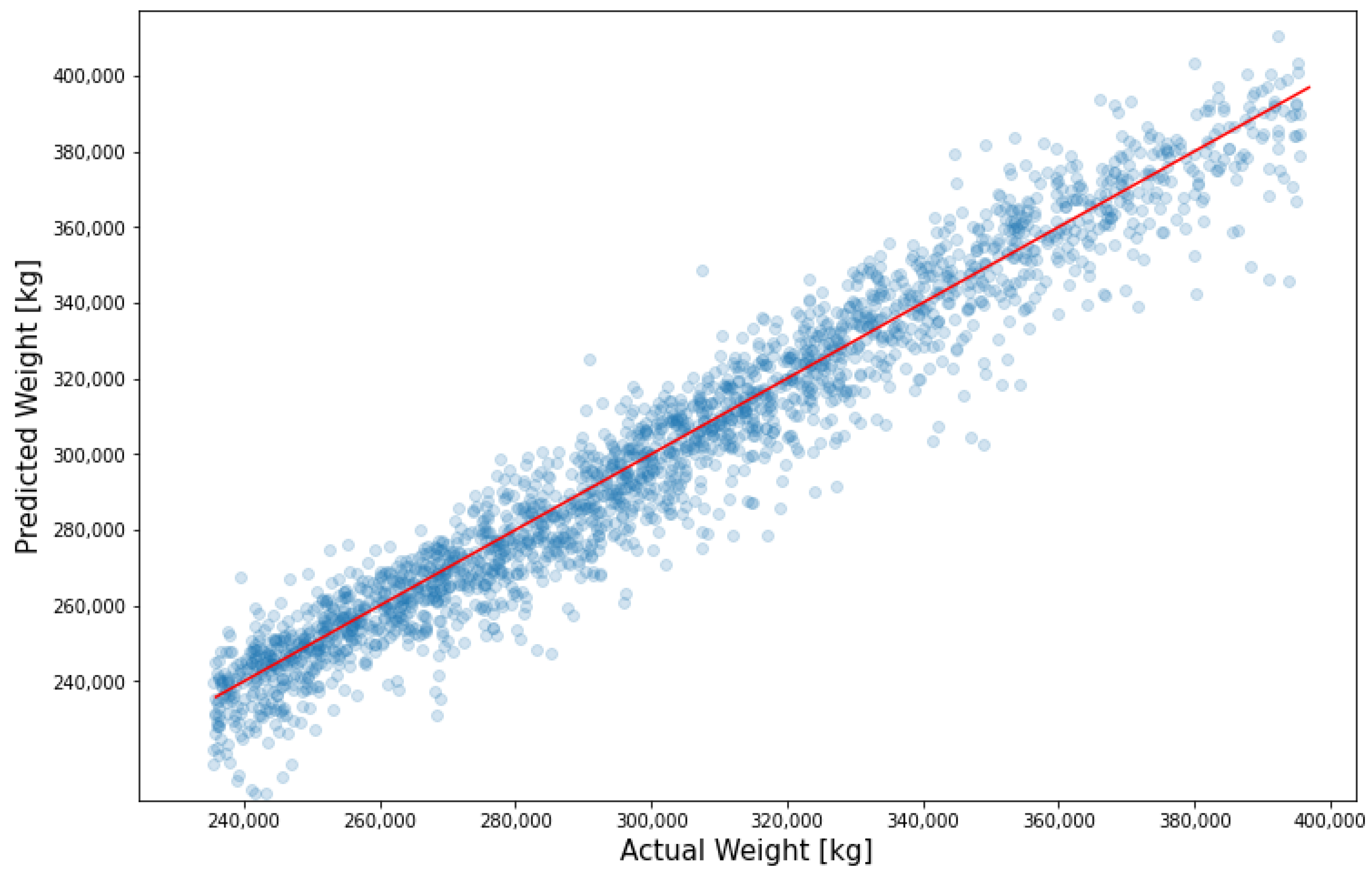
These give the model 27 inputs to work with. The model itself has an architecture containing 2 hidden layers with 32 nodes and the final output node which gives the estimated weight. Increasing the number of neurons in the hidden layers and number of layers was also tested, but this led to the model overfitting to the training data, which causes the accuracy to drop on the test data. The activation function used in each layer is ReLU [22] which yields better results compared to other activation functions and after each hidden layer, a dropout layer with 3% drop chance is added to prevent overfitting. Increasing the drop chance, does not increase the model’s performance on the test data and only decreases the accuracy on the training set. The model is then trained over three consecutive training sections with learning rates of 0.01, 0.001 and 0.0001, over 80% of the collected data, with a batch size of 32 samples. Figure 9 shows the result of the weight model predictions over the test sample which consists of 2667 flights in different airports than the training data with random weather conditions.
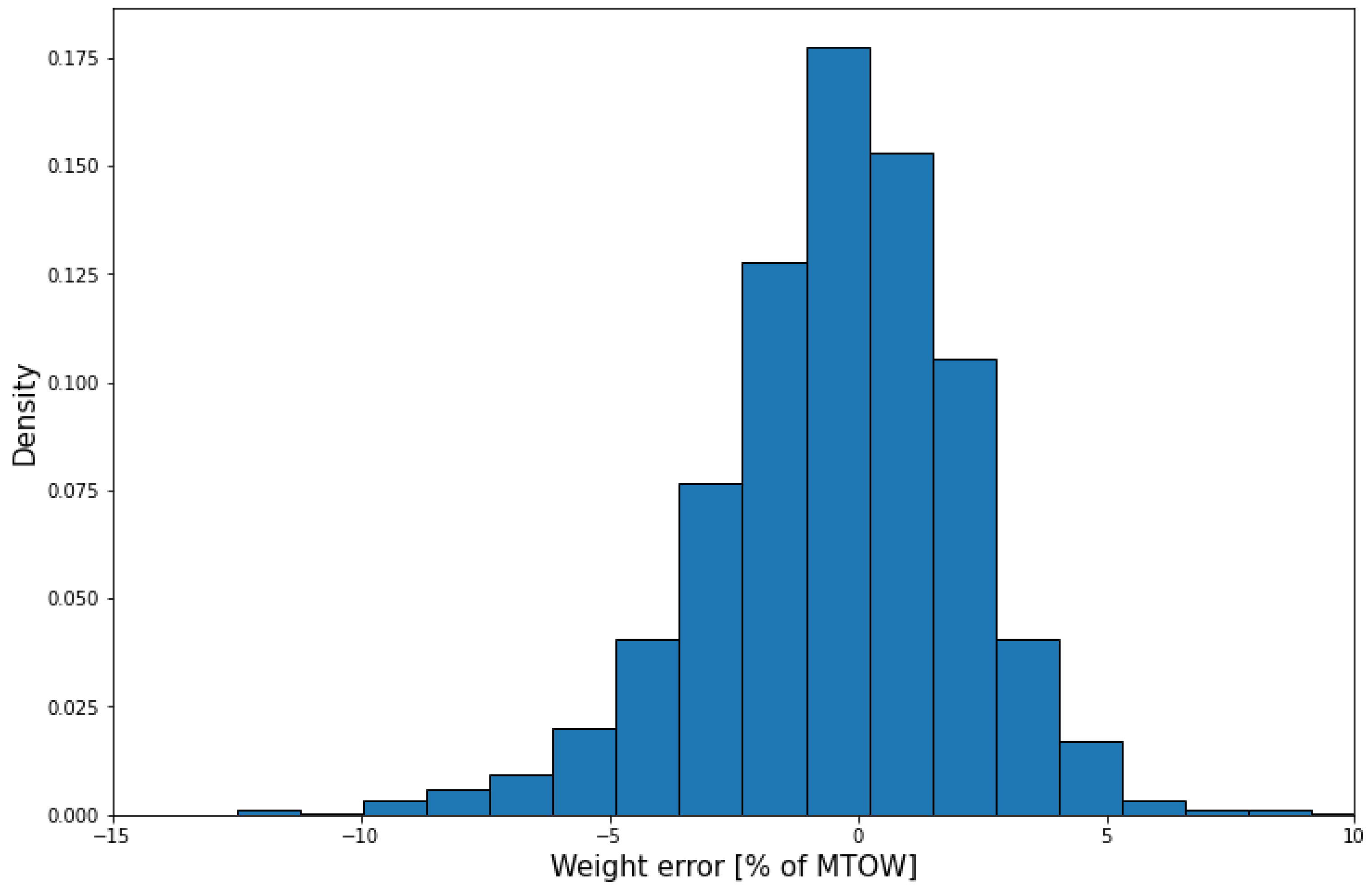
Distribution of the error is shown in Figure 10. The mean absolute error for the weight model is 1.97% of MTOW (maximum takeoff weight), with a standard deviation of 2.61% of MTOW.

4.2. Thrust Model

The real power of the method presented in this article is the ability to also predict the airplane’s thrust at each data point. The inputs used by this model are:
  • Total weight
  • Ground speed
  • Altitude above ground
  • Acceleration
  • Air temperature, pressure and density ratio
  • Climb angle
  • Bank angle
  • Wind speed
  • Cosine and sine of the angle between the wind direction and the aircraft heading
As observed, this model uses the total weight as an input which will be given from the output of the previous model when used on real flights, but for the purpose of training the model, the accurate weight at each point is given.
The architecture of the thrust model consists of an input layer with 12 inputs listed above, 4 hidden layers with 64, 64, 32 and 16 nodes and one final output node which will estimate the corrected thrust at each data point. The activation function used at each layer is sigmoid [22] and the training is carried out over three consecutive sessions with learning rates of 0.01, 0.001 and 0.0001, over 90% of the collected data, with a batch size of 256 samples. The increase in size of the thrust model compared to the weight model stems from the fact that this model is trained on each data point during the flight, while the weight model has only one data sample for each flight. So having access to a large set of data for training, the thrust model is designed to have more neurons and hidden layers to better be capable of generalizing. It also allowed the use of a larger portion of the collected data for training. The consecutive training sessions with different learning rates used for all the models is a well known method to fine tune the model with progressively more precision. Continuing the training with smaller learning rates seems to be ineffective in increasing the accuracy of the models.
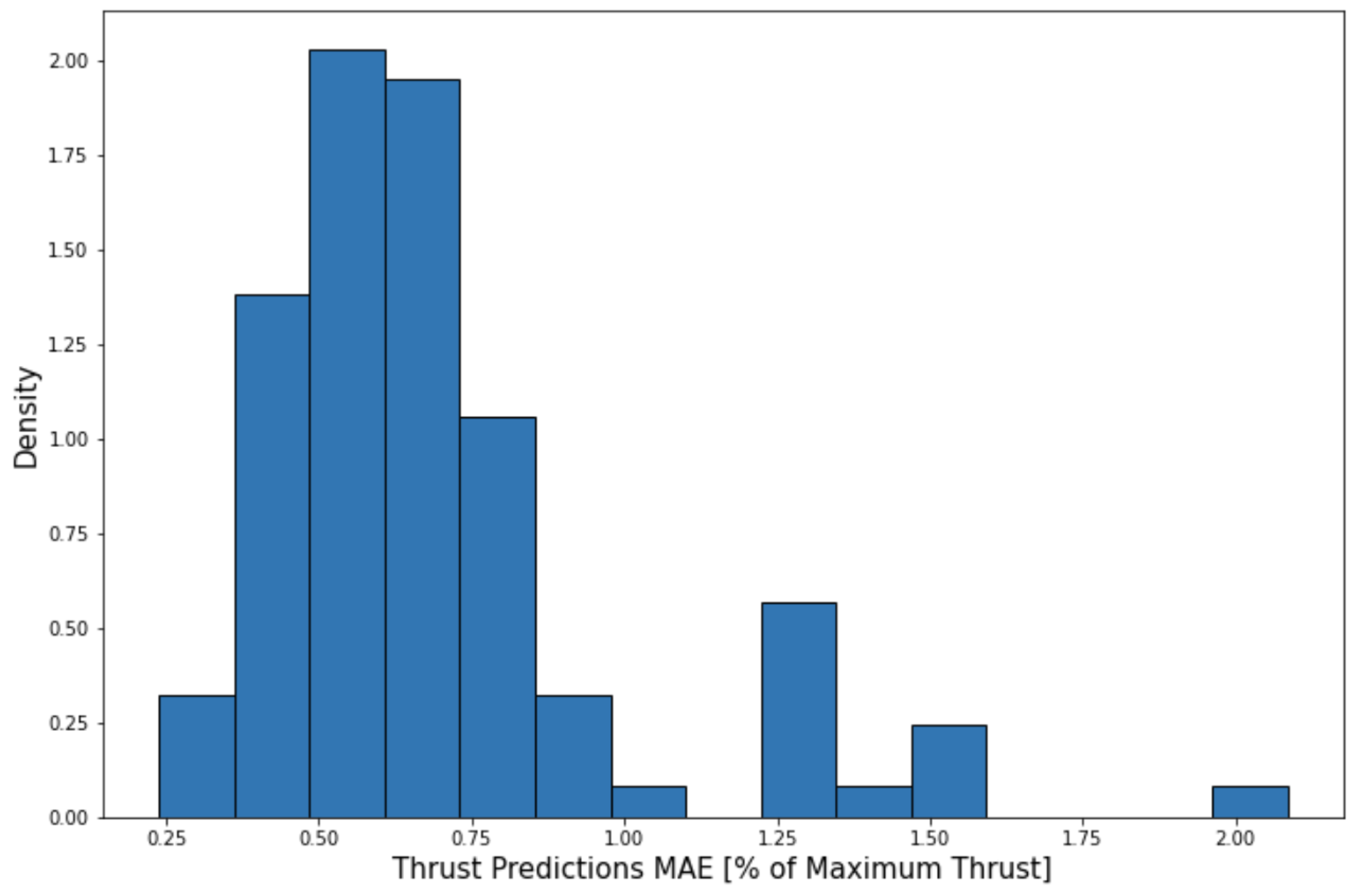
The resulting model is then tested on 1000 flights generated in new airports, with random weather conditions. For each flight, the thrust is estimated for each data point and then the mean absolute error of the predictions is calculated. The distribution of the error shown as a percentage of the maximum takeoff thrust is shown in Figure 11.
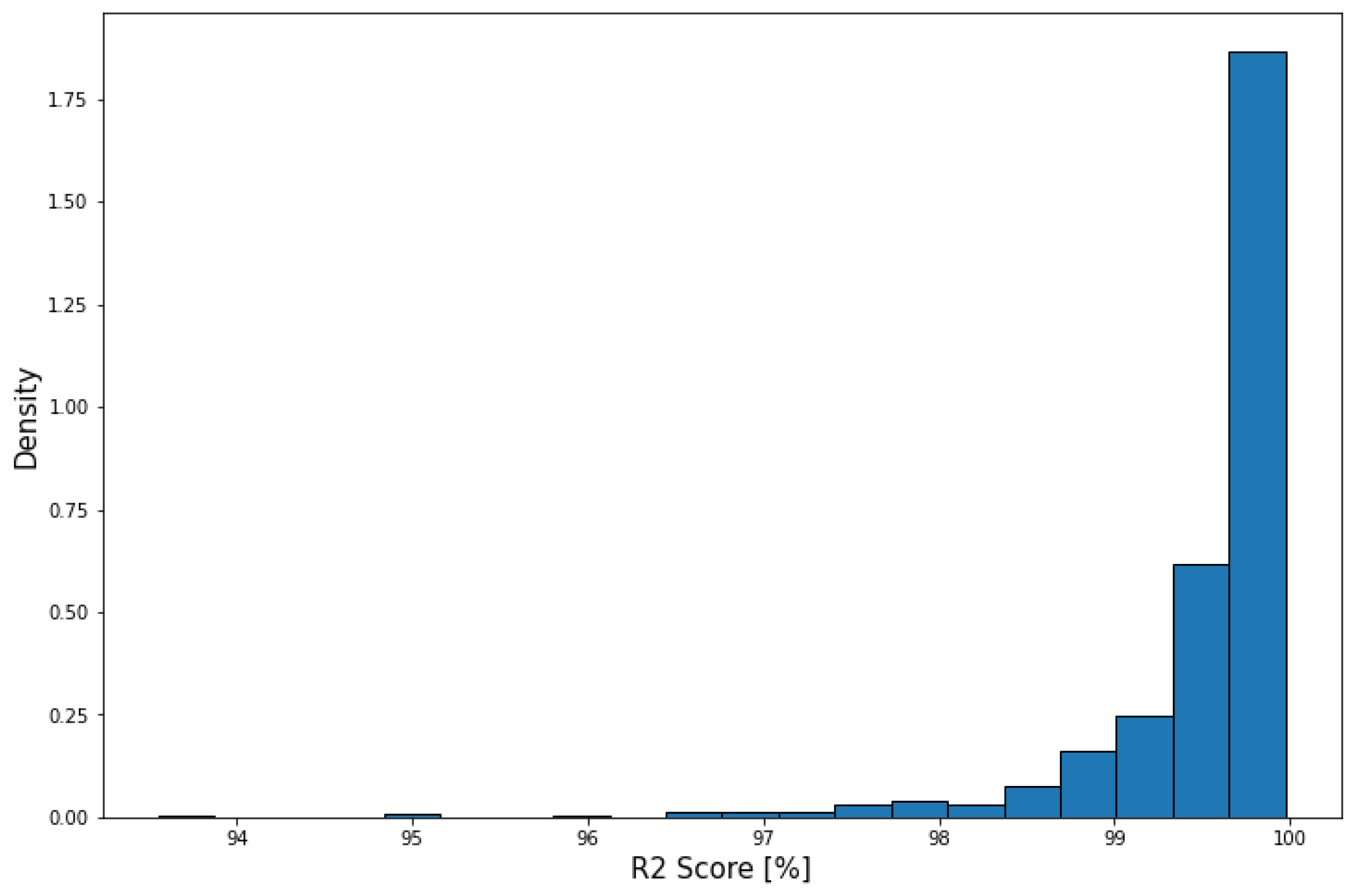
The average mean absolute error of thrust predictions for the 1000 flights is 0.70% of the maximum takeoff thrust with 0.31% standard deviation. Figure 12 shows the distribution of R2 score for these flights.
The predictions on average achieve a score of 98.62%, with a standard deviation of 1.27%.
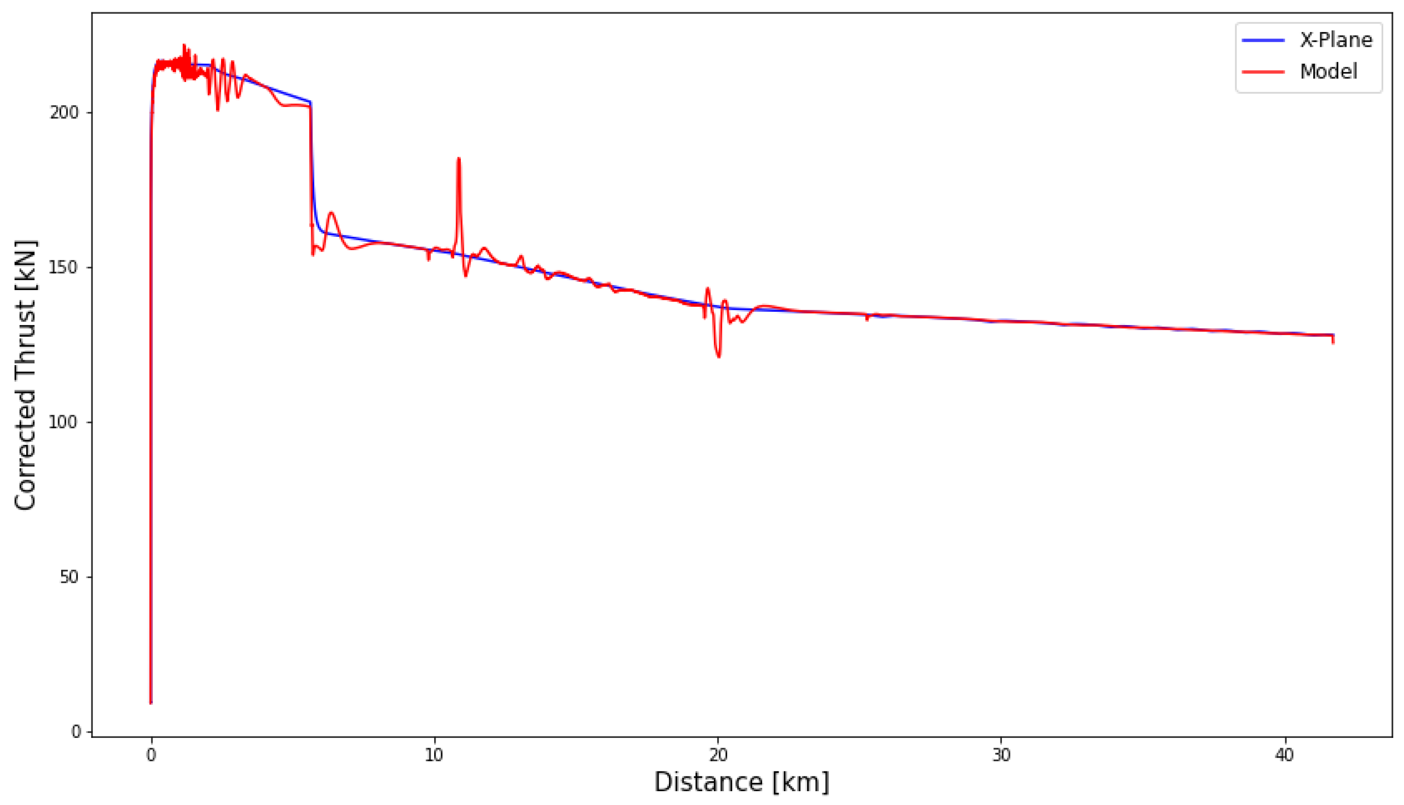
As an example, the corrected net thrust of one flight, estimated by the model at each data point is shown in Figure 13. The corrected net thrust is calculated by dividing the actual thrust over the square root of the air density ratio. As an example, the corrected thrust predictions for one of these flights is shown in the following plot.
The only parts containing some noise in the thrust predictions are in the beginning and where the flap settings are being changed during the acceleration segment.

4.3. Flap Model

The aim of this model is to predict the flap setting for each data point. For this purpose, unlike what is described before, because there is a limited number of flap settings available, a classification model is used. The inputs given to this model are identical to the thrust model, going through three hidden layers with 128, 64 and 32 nodes, with an output layer consisting of 6 nodes, each representing a different flap setting, from flap zero, to flap 20 and an extra option for the transient moments when the flaps are being retracted. The activation function used for the hidden layers is sigmoid which compared to the other activation functions slightly improves the performance, and a softmax [22] activation function is applied to the output layer. Every hidden layer also has a drop chance of 10% to avoid overfitting. The model is then trained over three consecutive training sessions with 0.1, 0.01 and 0.001 learning rates, over 90% of the collected data and with a batch size of 256 samples.
The trained flap model is used on flight data in a unique way in order to improve the accuracy of the predictions. First, the period in the middle of the flight, when the accelerations happen, is identified by considering a minimum acceleration value of 0.26 m·s−2. Since the flap setting is changed on a specific schedule based on calibrated air speed [14], which only changes during acceleration segments, during the first climb the flap setting is constant and therefore the predictions for this segment can be averaged to yield the final flap setting prediction. Then in the period between the start of the first acceleration and the end of last acceleration, the predictions are again averaged but over 12 s around the point. This value is chosen not randomly but by considering the average time lapse in ADS-B data, which allows the model to most likely average the predictions for three data points when used on ADS-B data. However, for the purpose of testing the models, all the predictions are done over the regular X-Plane data which on average have a time step of 0.1 s. At last, after the last acceleration, without using the model, the predictions are set to zero for the flap setting, since at the end of acceleration in reality and in the simulations the flaps are reduced to zero.
Table 2 shows the accuracy of the model used in the aforementioned fashion, over test flights not previously seen by the model. Each row shows the actual flap setting and each column represents the predicted flap setting. All the values are in percentage of total number of each flap setting.
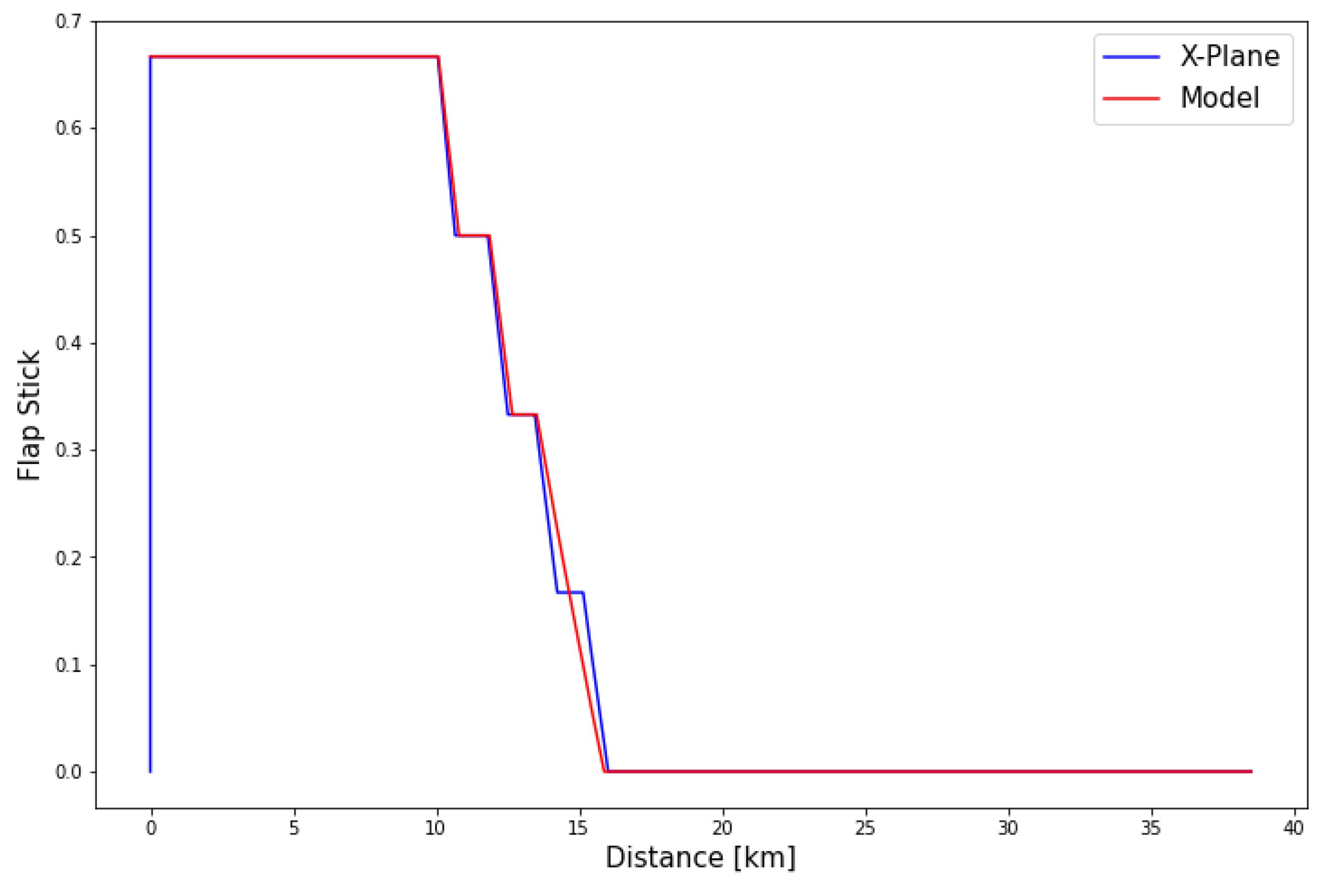
To show the progression of flap setting through time in a flight, the scalar value introduced in Table 1 is used. Consequently, the overall performance of the model in predicting flap settings for each flight can be assessed through the R2 score of predictions for each flight shown in Figure 14. The average R2 score is 99.52% with a standard deviation of 0.61%, which means the model accompanied by the algorithm explained above can almost predict the flap setting perfectly. It is worth mentioning that the takeoff flap setting for these flights was predicted with 100% accuracy. As an example, the flap predictions for a single flight are shown in Figure 15.

5. Results

While X-Plane gives the values for climb angle and bank angle directly, these values have to be estimated using the position and velocity from the given radar/ADS-B data. Furthermore, the time interval between data points is about 0.1 s in X-Plane, which gives much better precision in calculating the acceleration at each point, while the larger time increment available from the real data reduces the accuracy.
In order to have a more precise assessment of the models’ capability, in this section, first an approach to replicating the ADS-B data is explained, then for each flight the output of the weight model is given to the thrust and flap models to then estimate the corrected thrust and flap setting for each data point. Then the same procedure is repeated to assess the model capabilities on radar data which has 4 s intervals between data points.

5.1. X-Plane Data with ADS-B Format

For transforming the X-Plane data into a format closer to the ADS-B flight data 13,809 ADS-B departure data for a variety of aircraft types and at the airports of AMS and CDG are analyzed and the distribution of the time difference between data points in four different altitude ranges is shown in Figure 16.
Examining the collected data, there is a change in the time increment distribution above 1524 m altitude, which in Figure 17 is shown more clearly. The exact distributions in Figure 17 are used to generate random time increments.
The variables affected by this transformation are acceleration, climb angle and bank angle, because even though these values are known exactly from X-Plane, in reality the acceleration and climb angle at each point is calculated using the position and velocity at each data point and the bank angle is unknown. The formula used to have an estimate of the bank angle is taken from [16], which uses the ground speed V, the turn radius r and the gravitational acceleration g, as seen in the equation below.
ϵ = arctan ( 2.85 V 2 r g )
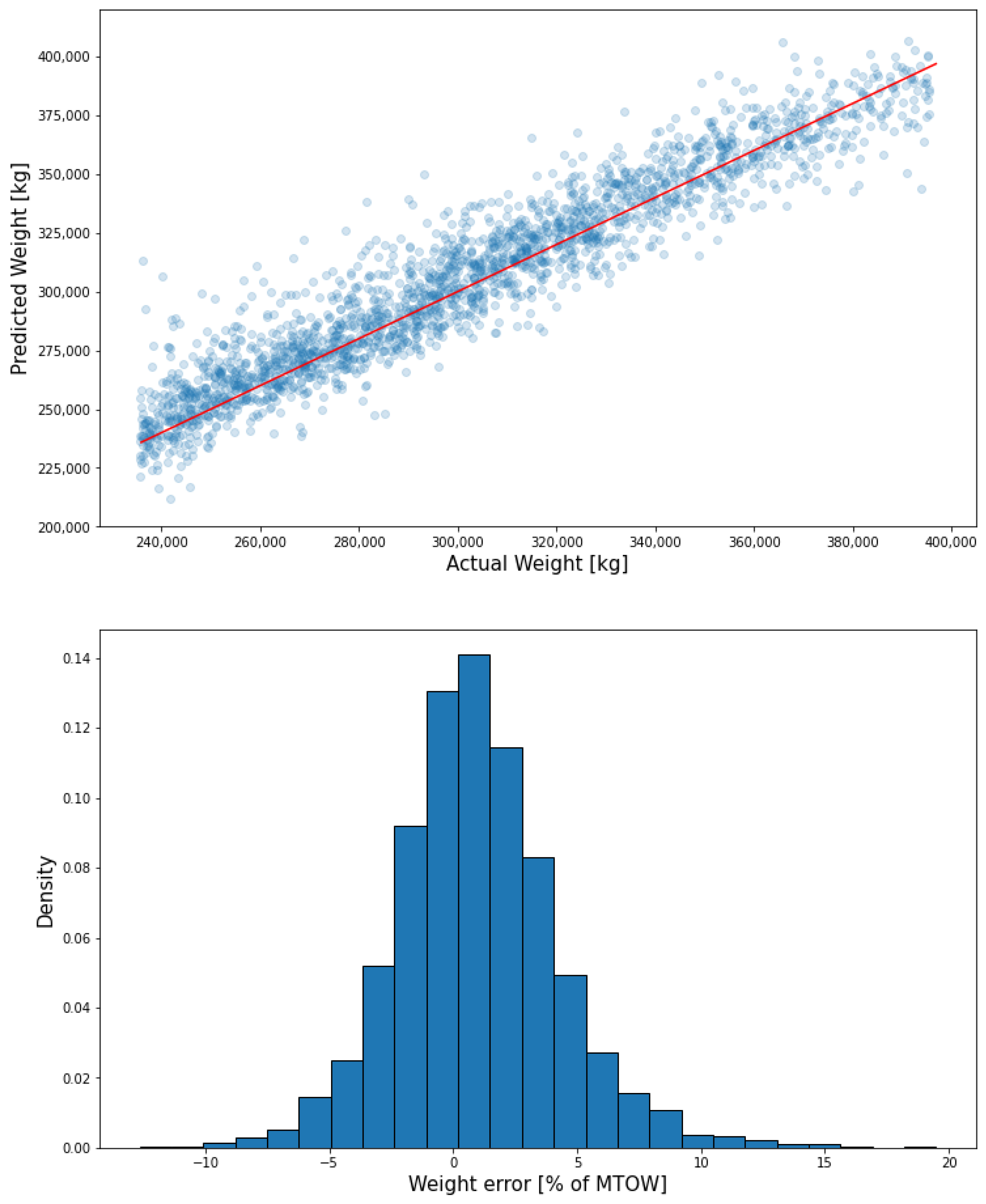
The models are then tested on 2204 flights not previously seen, which have been transformed into ADS-B format using the time interval distribution above. The average run-time per flight was 0.1330 s, on a device with AMD Ryzen 7 5800H CPU. Figure 18 shows the performance of the weight model on the data. The average weight error is 2.63% of MTOW, with standard deviation of 2.39%, which shows that even though with respect to the accurate data the accuracy is lower, it is still in a desirable range.
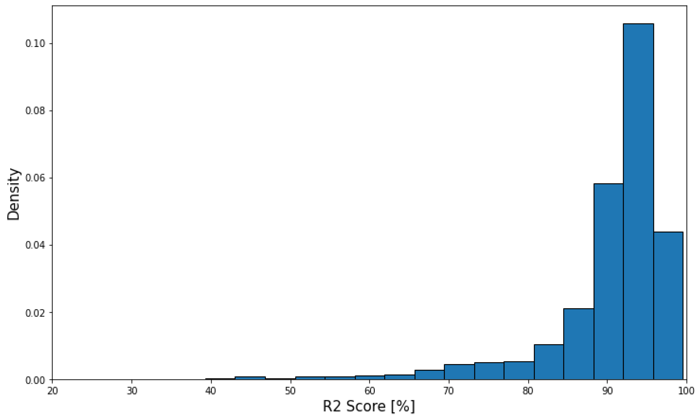
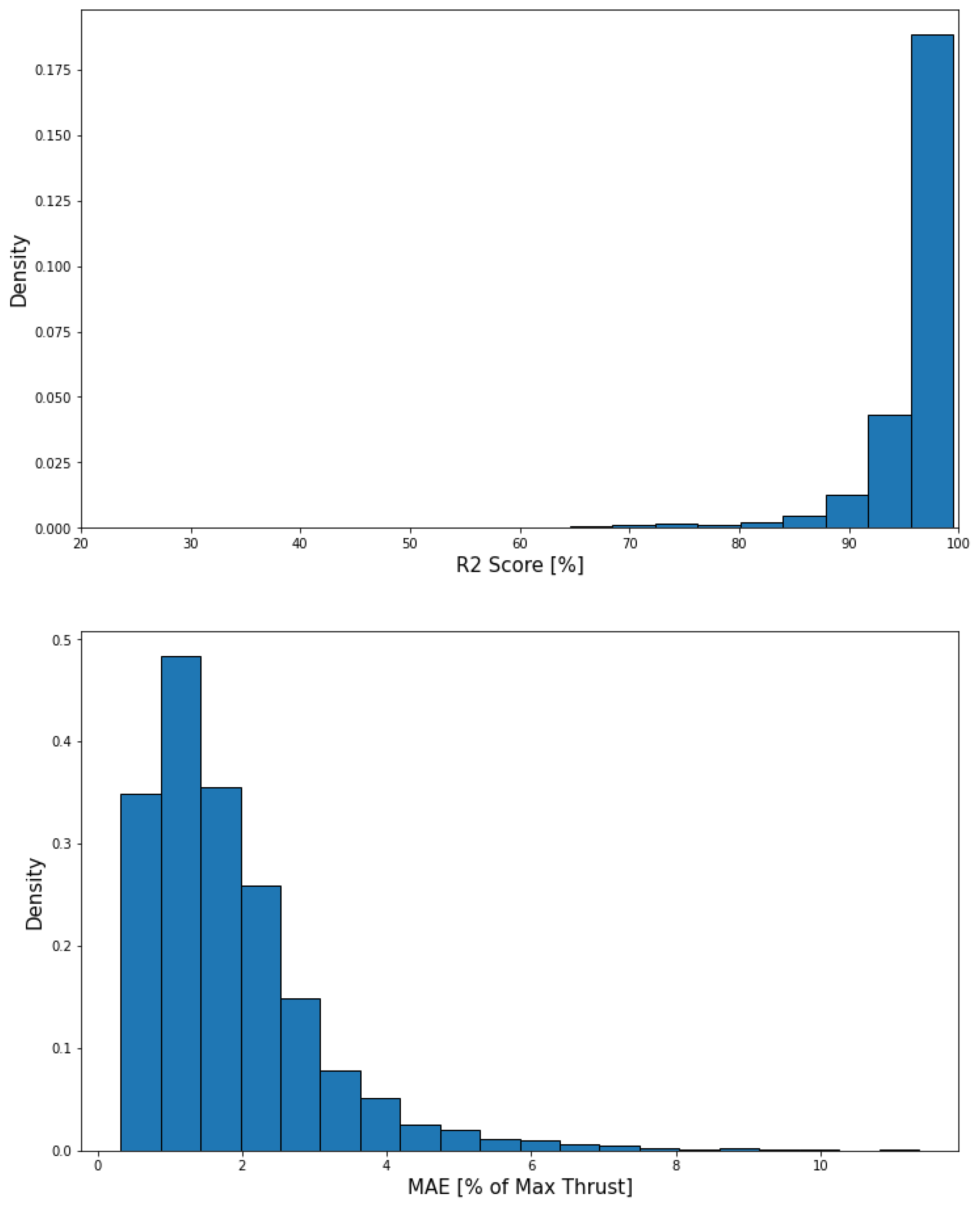
Figure 19 shows the performance of the thrust model. The average R2 score of thrust predictions is 89.90% and the average mean absolute error is 2.74% of maximum thrust. So understandably, since the thrust model had almost zero error with the accurate inputs, the error now closely follows the weight model error.
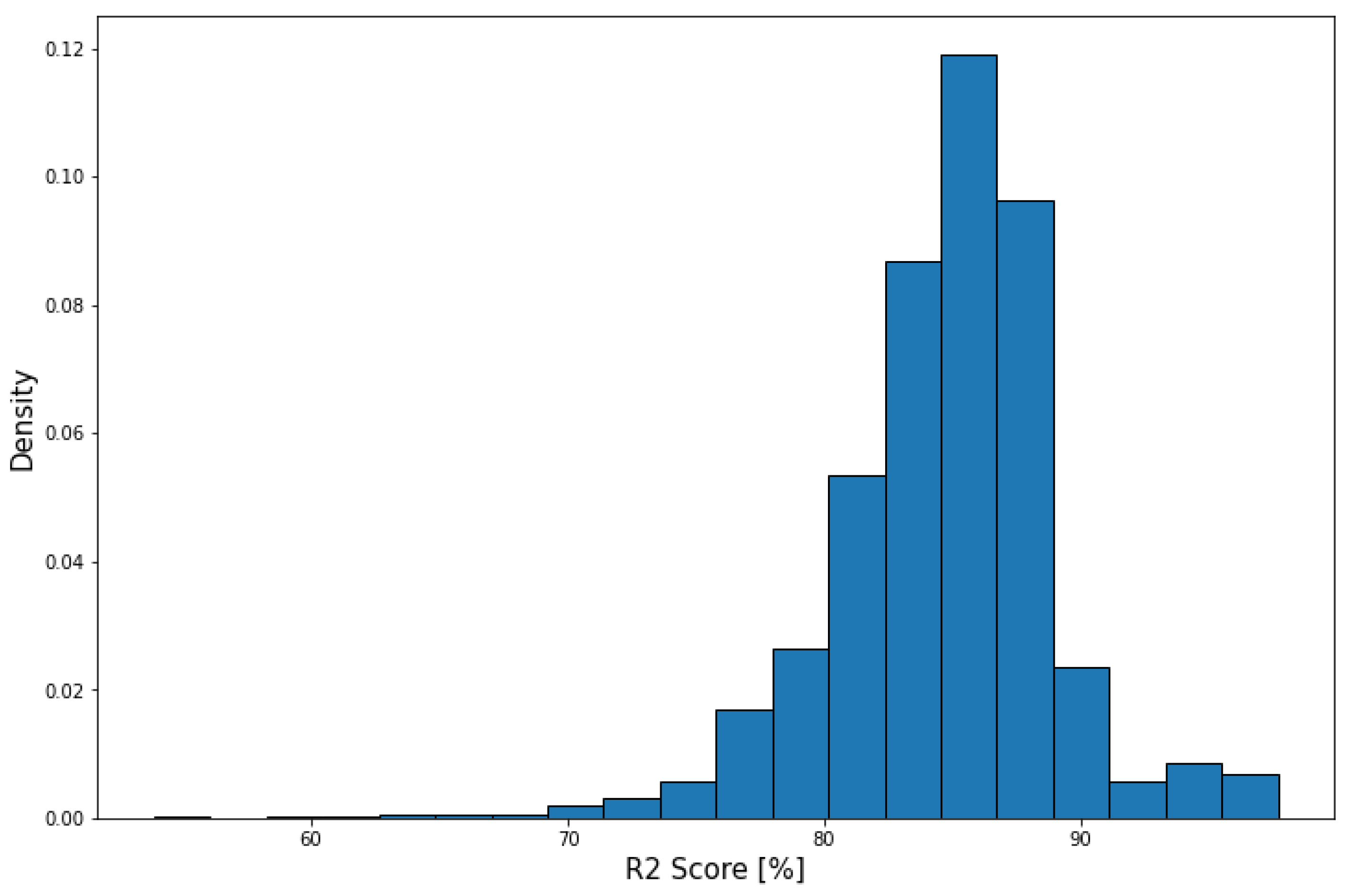
Finally, Figure 20 shows the performance of the flap model and the average R2 score for this model is 84.68%, with 99.95% accuracy on predicting the takeoff flap setting. Since the method used by the flap model is to average the outputs for a period of time around the desirable data point, the scarcity of data points in this format causes this model’s performance to have the biggest difference with respect to the tests carried out on accurate data.

5.2. X-Plane Data with Radar Format

Unlike the ADS-B format, which has a wide range of time increments, the radar format has a constant time interval between data points and for this purpose according to [16] a time interval of 4 s is considered between data points. Following the same procedure explained in the previous section, the models are tested again but this time on the test data modified according to the radar format. The average run-time per flight was 0.1534 s. The reason for this number being higher than the previous format is that the smaller time increments of radar data make it so that the number of data points on average for a flight is higher; hence, the average run-time for the radar data is higher than the ADS-B format.
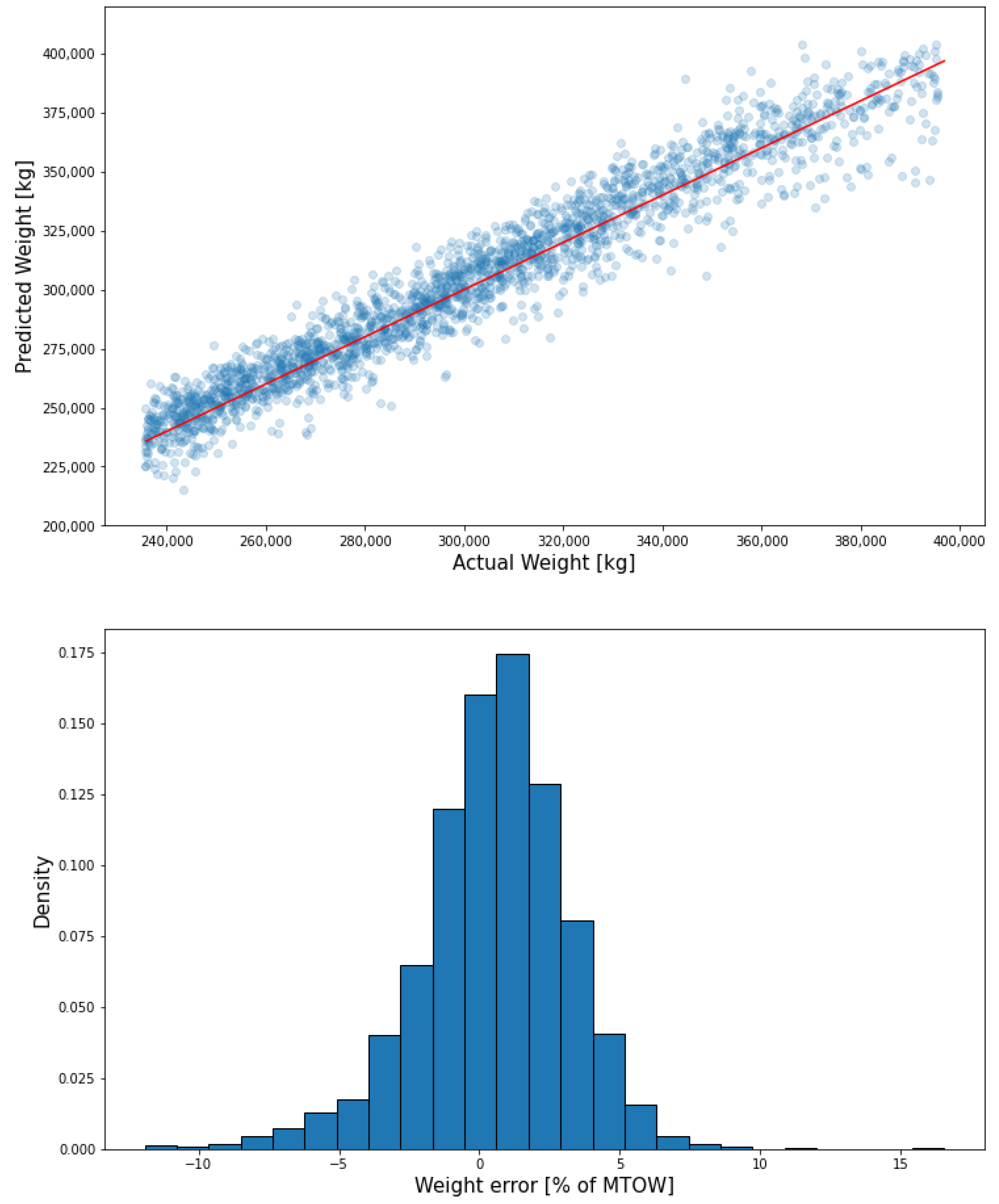
Figure 21 shows the performance of the weight model on the data. The mean absolute error for the weight predictions in this case is 2.07% of MTOW, with a standard deviation of 1.65%, which as expected is better than the performance on the data with ADS-B format, since the radar data have better quality due to the time increments being smaller.
Furthermore, the performance of the thrust model is shown in Figure 22 and the data show the mean absolute error to be 1.84% of maximum thrust on average with an R2 score of 95.56%, which are again higher than the previous format.
Lastly, Figure 23 shows the R2 score distribution of the flap setting predictions, which gives an average of 88.24%, with 99.96% takeoff flap setting prediction accuracy.
These results suggest that the methodology presented in this article is capable of predicting the weight, thrust profile and flap setting for a given flight, by only using available data from radar or ADS-B data formats, with good accuracy and in a reasonably short time. Furthermore, no excess information regarding the aerodynamic properties of the airplane such as coefficients of lift and drag is needed for the models to predict the desired outputs and the outputs are estimated only using weather data and the position and velocity of the airplane over time. However, further analysis and testing on real data taken from the Flight Data Recorder (FDR) is needed to fully validate the models.
In the future, the study could be extended to many other airplane models and there is also the possibility of adding arrival flights to develop models that predict the same outputs but by taking in the landing data from radar or ADS-B.

6. Conclusions

This paper presents a methodology to estimate an aircraft’s takeoff weight, thrust and flap settings using neural network models. First, the neural network models were trained on flights generated using a flight simulator. Then, the performance of the models was assessed on the test dataset transformed in a way to replicate ADS-B and radar data formats, to prove that it can estimate the three parameters with a reasonable degree of uncertainty, even on low quality data. The average run-time per flight for the ADS-B format was 0.1330 s and 0.1534 s for the radar format. Table 3 shows a summary of the results.
The first column shows the results when the accurate inputs have been given to the models with 0.1 s time intervals. For the other two, surveillance data are replicated using the X-Plane data, then they are first given to the weight model. Using the output of the weight model, then the thrust and flap models predict the outputs, which are then compared to the actual thrust level and flap setting. Hence, the accuracy of the thrust and flap models is affected by the error coming from the weight model. As expected, the flap model is affected the most by the drop in data quality, as the predictions are based on averaging the outputs in a 12 s time period around each point and when the time increment increases, as is the case for surveillance data, there are fewer data points in this period and the accuracy drops as well.
Overall, the results show a promising method for predicting the weight, thrust level and flap setting of a given flight, without having access to accurate FDR data and only using surveillance data.

Author Contributions

Conceptualization, K.A. and M.C.; formal analysis, K.A.; writing—original draft preparation, K.A.; writing—review and editing, K.A. and M.C.; visualization, K.A.; supervision, M.C. All authors have read and agreed to the published version of the manuscript.

Funding

This research received no external funding.

Institutional Review Board Statement

Not applicable.

Informed Consent Statement

Not applicable.

Data Availability Statement

The data presented in this study are available on request from the corresponding author. The data are not publicly available due to confidentiality.

Acknowledgments

The authors would like to express their sincere gratitude to Ben Romarowski for his contribution in conceiving the initial idea for this project.

Conflicts of Interest

The authors declare no conflict of interest.

References

  1. International Civil Aviation Organization. Recommended Method for Computing Noise Contours around Airports; Technical Report Doc. 9911; ICAO: Montreal, Canada, 2018. [Google Scholar]
  2. Aircraft Noise Model. The Aircraft Noise and Performance (ANP) Database. Available online: http://www.aircraftnoisemodel.org (accessed on 22 March 2022).
  3. International Civil Aviation Organization. ICAO Aircraft Engine Emissions Databank. 2022. Available online: https://www.easa.europa.eu/domains/environment/icao-aircraft-engine-emissions-databank (accessed on 25 March 2022).
  4. EUROCONTROL. User Manual for the Base of Aircraft Data (BADA), Rev 3.12. 2014. Available online: https://www.eurocontrol.int/publication/user-manual-base-aircraft-data-bada-revision-38 (accessed on 27 March 2022).
  5. Alligier, R.; Gianazza, D.; Durand, N. Learning the Aircraft Mass and Thrust to Improve the Ground-Speed Trajectory Prediction of Climbing Flights. Transp. Res. Part C Emerg. Technol. 2013, 36, 45–60. [Google Scholar] [CrossRef]
  6. Alligier, R.; Gianazza, D.; Durand, N. Machine Learning and Mass Estimation Methods for Ground Based Aircraft Climb Prediction. IEEE Trans. Intell. Transp. Syst. 2015, 16, 3138–3149. [Google Scholar] [CrossRef]
  7. Schultz, C.; Thipphavong, D.; Erzberger, H. Adaptive Trajectory Prediction Algorithm for Climbing Flights. In Proceedings of the AIAA Guidance Navigation and Control (GNC) Conference, Minneapolis, MN, USA, 13–16 August 2012; p. 2. [Google Scholar]
  8. Sun, J.; Ellerbroek, J.; Hoekstra, J. Modelling and inferring aircraft takeoff mass from runway ADS-B data. In Proceedings of the 7th International Conference on Research in Air Transportation, Philadelphia, PA, USA, 20–24 June 2016. [Google Scholar]
  9. Sun, J.; Ellerbroek, J.; Hoekstra, J. Aircraft initial mass estimation using Bayesian inference method. Transp. Res. Part C Emerg. Technol. 2018, 90, 59–73. [Google Scholar] [CrossRef]
  10. Sun, J.; Blom, H.; Ellerbroek, J.; Hoekstra, J. Aircraft mass and thrust estimation using recursive Bayesian method. In Proceedings of the 8th International Conference on Research in Air Transportation (ICRAT2018), Catalonia, Spain, 26–29 June 2018. [Google Scholar]
  11. Jarry, G.; Delahaye, D.; Feron, E. Approach and landing aircraft on-board parameters estimation with LSTM networks. In Proceedings of the 2020 International Conference on Artificial Intelligence and Data Analytics for Air Transportation (AIDA-AT), Singapore, 3–4 February 2020. [Google Scholar]
  12. Barros dos Santos, S.R.; Givigi, S.; Nascimento, C., Jr.; Bittar, A.; Oliveira, N. Modelling of a Hardware in the Loop Simulator for UAV Autopilot Controllers. In Proceedings of the 21st Brazilian Congress of Mechanical Engineering, Natal, Brazil, 24–28 October 2011; Voluem 6, pp. 1301–1315. [Google Scholar]
  13. Bangga, G. Comparison of Blade Element Method and CFD Simulations of a 10MW Wind Turbine. Fluids 2018, 3, 73. [Google Scholar] [CrossRef]
  14. International Civil Aviation Organization. Review of Noise Abatement Procedure Research and Development and Implementation Results; Discussion of Survey Results; ICAO: Montreal, Canada, 2007. [Google Scholar]
  15. PMDG. Boeing 747-400 Flight Manual, Revision 26th ed.; PMDG: Las Vegas, NV, USA, 2006. [Google Scholar]
  16. European Civil Aviation Conference. Volume 2: Technical Guide. In Methodology for Computing Noise Contours around Civil Airports; Technical Report CEAC Doc.29; ECAC: Neuilly-sur-Seine, France, 2016. [Google Scholar]
  17. FlightRadar24. Flight Tracking Data. Available online: https://www.flightradar24.com (accessed on 22 March 2022).
  18. Federal Aviation Administration. Pilot’s Handbook of Aeronautical Knowledge (FAA-H-8083-25B); U.S. Department of Transportation, Federal Aviation Administration: Washington, DC, USA, 2016; Chapter 14.
  19. Office of Aviation Research Washington DC. Statistical Data for the Boeing 747-400 Aircraft in Commercial Operations; Technical Report FAA-AR-05-3; Federal Aviation Administration: Washington, DC, USA, 2005.
  20. Advisory Circular AC 25-13; Technical Report; US Department of Transportation, Federal Aviation Administration: Washington, DC, USA, 1988.
  21. Boeing. Onboard Performance Tool (OPT) for 737, 747, 757, 767 and 777 Airplanes; Boeing: Arlington, VA, USA, 2013. [Google Scholar]
  22. Goodfellow, I.; Bengio, Y.; Courville, A. Deep Learning; MIT Press: Cambridge, MA, USA, 2016. [Google Scholar]
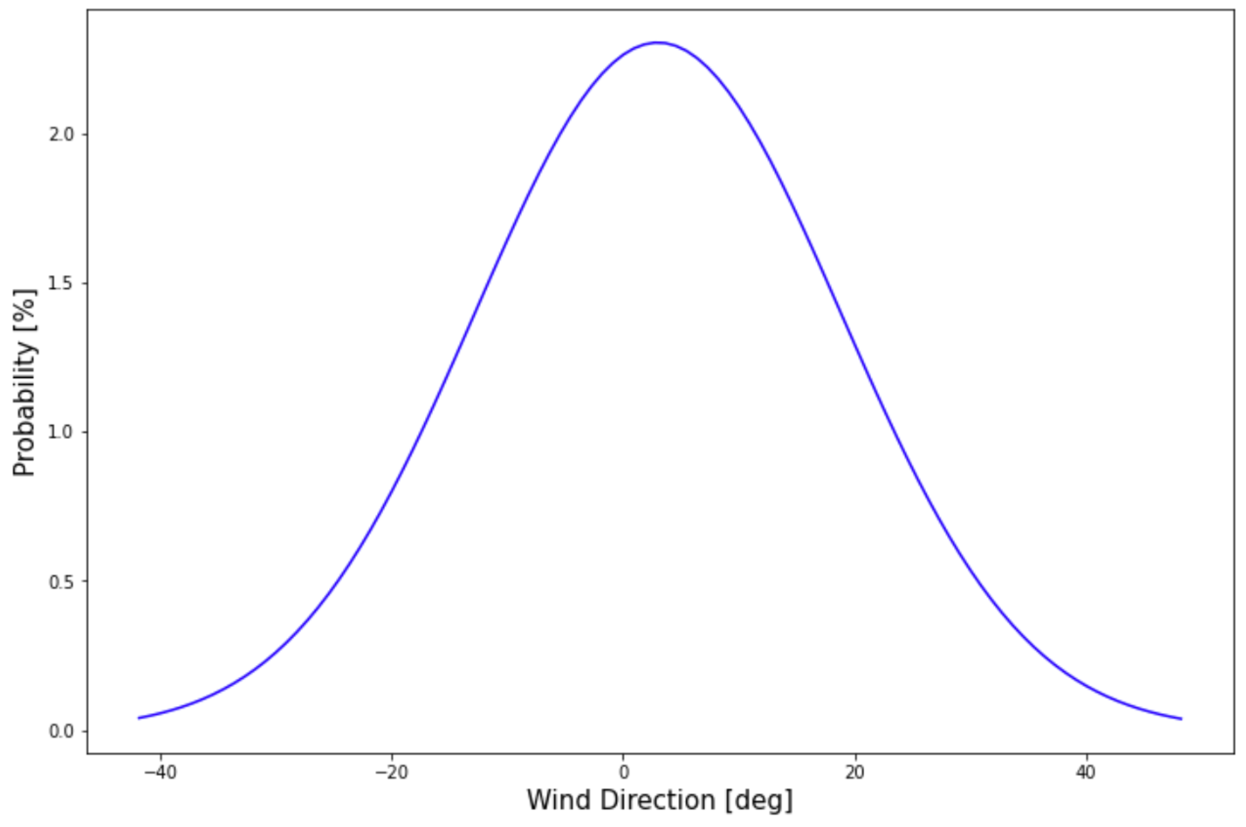
Figure 1. Generated wind direction distribution for Schiphol airport.
Aerospace 10 00513 g001
Figure 2. Throttle controller performance.
Aerospace 10 00513 g002
Figure 3. Rudder controller performance.
Aerospace 10 00513 g003
Figure 4. Climb angle controller performance.
Aerospace 10 00513 g004
Figure 5. Bank angle controller performance.
Aerospace 10 00513 g005
Figure 6. Generated flight paths up to 3048 m.
Aerospace 10 00513 g006
Figure 7. Generated flight paths up to 1524 m.
Aerospace 10 00513 g007
Figure 8. Climb angle distribution comparison.
Aerospace 10 00513 g008
Figure 9. Weight model predictions.
Aerospace 10 00513 g009
Figure 10. Weight prediction error distribution.
Aerospace 10 00513 g010
Figure 11. Thrust prediction error distribution.
Aerospace 10 00513 g011
Figure 12. Thrust prediction R2 score distribution.
Aerospace 10 00513 g012
Figure 13. Thrust predictions for a single flight.
Aerospace 10 00513 g013
Figure 14. Flap predictions, R2 score distribution.
Aerospace 10 00513 g014
Figure 15. Flap setting predictions, for a single flight.
Aerospace 10 00513 g015
Figure 16. Time increment box plot for different altitude ranges.
Aerospace 10 00513 g016
Figure 17. Time increment distribution for above and below 1524 m.
Aerospace 10 00513 g017
Figure 18. Weight model performance on X-Plane data with ADS-B format.
Aerospace 10 00513 g018
Figure 19. Thrust model performance on X-Plane data with ADS-B format.
Aerospace 10 00513 g019aAerospace 10 00513 g019b
Figure 20. Flap model performance on X-Plane data with ADS-B format.
Aerospace 10 00513 g020
Figure 21. Weight model performance on X-Plane data with radar format.
Aerospace 10 00513 g021
Figure 22. Thrust model performance on X-Plane data with radar format.
Aerospace 10 00513 g022
Figure 23. Flap model performance on X-Plane data with radar format.
Aerospace 10 00513 g023
Table 1. Flap retraction schedule.
Flap IDFlap ValueV2+
0080
10.16760
50.33340
100.50020
200.6670
Table 2. Flap prediction confusion matrix.
Actual/Predicted0151020Retract
092.561.090006.35
13.0570.110.590026.25
502.9377.041.23018.80
10000.5094.863.321.41
200009.2090.610.19
Retract11.4117.935.533.611.0060.52
Table 3. Summary of the models’ performance.
MetricAccurate InputsADS-B ReplicaRadar Replica
Weight MAE (% of MTOW)1.972.582.07
Thrust MAE (% of Max Thrust)0.702.721.84
Thrust Average R2 Score (%)98.6289.9095.56
Flap Average R2 Score (%)99.5184.7088.24
Takeoff Flap Prediction Accuracy (%)100.0099.9599.96
Disclaimer/Publisher’s Note: The statements, opinions and data contained in all publications are solely those of the individual author(s) and contributor(s) and not of MDPI and/or the editor(s). MDPI and/or the editor(s) disclaim responsibility for any injury to people or property resulting from any ideas, methods, instructions or products referred to in the content.