Article

NARX-Elman Based Mach Number Prediction and Model Migration of Wind Tunnel Conditions

College of Information Science and Engineering, Northeastern University, Shenyang 110819, China
*
Author to whom correspondence should be addressed.
Aerospace 2023, 10(6), 498; https://doi.org/10.3390/aerospace10060498
Submission received: 6 April 2023 / Revised: 12 May 2023 / Accepted: 21 May 2023 / Published: 25 May 2023
(This article belongs to the Section Aeronautics)

Abstract

:
Mach number, as an important index to judge the system performance in wind tunnel tests, its stability determines the quality of the flow field of this wind tunnel and needs to be controlled precisely. Due to the complex process in the wind tunnel test, it is difficult to ensure the smooth operation of the Mach number by the traditional control strategy, therefore, a Mach number prediction model based on a nonlinear autoregressive exogenous model (NARX)-Elman is proposed in this paper. Firstly, the NARX model is adopted as the basic framework of this model, the false nearest neighbor (FNN) is used for model order solving, and the Elman network is used for dynamic nonlinear fitting of the model. Secondly, considering the wind tunnel system with multiple conditions and the high cost of conducting complete data experiments, a new model migration method, the input-output slope/bias correction-genetic algorithm (IOSBC-GA), is proposed, which uses IOSBC method as the basic framework to construct the migration model based on the historical condition model and a small amount of data of the new condition, and uses GA to find the slope of deviation in the new model and correct the input-output relationship between the old and new conditions, so as to establish the model for the new condition. By comparing the model respectively with the traditional algorithm and the model built without migration, the root mean square error (RMSE) and the maximum deviation (MD) of this model are less than 0.001, indicating that the model has high prediction accuracy.

1. Introduction

Wind tunnel experiments have played a major role in exploring the nature of airflow, verifying the correctness of aerodynamic theoretical analysis and calculation results, and providing aerodynamic data for the development and modification of aircraft, missiles, and other vehicles. With the development of various new aerospace vehicles, the requirements for wind tunnel tests are increasing, and wind tunnels have become the most important experimental equipment indispensable for studying the aerodynamic characteristics of advanced vehicles [1]. Many important aerodynamic theories are inseparable from wind tunnel tests and also need to be verified by wind tunnel tests.
However, in wind tunnel experiments, due to the complexity of airflow, a variety of factors need to be considered, such as wind tunnel parameter settings, control strategies, sensor installation, etc., to ensure the accuracy and reliability of the experiments. For the control strategy in wind tunnel experiments, there are many alternative methods available. For example, traditional PID controllers, fuzzy controllers, neural network controllers, adaptive control, model predictive control, etc. For example, Shahrbabaki et al. designed a small low-speed wind tunnel system based on fuzzy control theory using artificial neural networks (ANN) to find the optimal membership function for a fuzzy logic controller (FLC) system [2]. Haley et al. designed a generalized predictive controller based on a linear predictor model, which successfully suppressed the drift of all testable Mach numbers and dynamic pressures across the speed of sound region [3]. Luo et al. proposed a new strategy of fuzzy and PID compounding for the high targets of capacity, pressure and Mach number in a 0.6 m wind tunnel and designed the corresponding controller, with a control accuracy of 0.2% [4].
During the wind tunnel operation, Mach number is an important performance index, of which stability and rapidity have an important influence on the wind tunnel flow field quality. In order to simulate the change of airflow in different directions during the operation of the vehicle, the angle of the vehicle needs to be changed after the Mach number reaches a preset stability point. The change in the angle of attack will have a great impact on the Mach number, and the system will be disturbed when the angle of attack is changed, making it difficult to maintain the Mach number within the required accuracy. This stage is the most important part of the whole blowing test and requires the controller to use a well-designed control system to adjust the Mach number to the required accuracy range. However, the change pattern of the wind tunnel flow field is rapid and complex, and improving the control accuracy of the Mach number has been a difficult problem for wind tunnel control [5].
In the early stage of Mach number control in wind tunnels, the most common control method is the traditional PID algorithm [6], but with the increasing requirements of control accuracy, the traditional PID control algorithm has been difficult to meet the basic requirements of control accuracy. At the same time, with the increasing demand of the system, the design structure has become more and more complex, and the nonlinearity, time lag, multiple conditions, multiple variables, and high accuracy requirements of the wind tunnel system make Mach number control more and more difficult [7]. Currently, for the above Mach number control difficulties and experimental analyses of a large amount of data, researchers have found that advanced control can solve the above problems [8]. The main principle of predictive control as one of the advanced control methods is to solve the control rate using an optimization method according to the dynamic change trend of the controlled object. This method is able to regulate the controlled process with time lags and to reduce or even avoid coupling between variables. In a predictive control system, the predictive model is crucial, and its prediction has an impact on the subsequent control solution and the final output change. The main function of the predictive model is to predict the future output of the object based on its historical information so that the direction of the controlled object can be known in advance to optimize the control and improve the control accuracy. For example, Jian Zhang, Ping Yuan et al. designed a flow field controller within the framework of predictive control without any offset model, using an augmented model approach to cope with other unknown disturbances and model mismatch to improve the control accuracy [9].
Wind tunnel research has developed to the point where there are two mainstream methods of predictive model building, one is mechanistic modeling [10], which focuses on establishing an aerodynamic model by analyzing the wind tunnel circulation structure, operational characteristics, etc., and can directly and explicitly describe the wind tunnel system. Another approach is data-driven modeling [11], which considers the whole system as a “black box” and uses the data collected in the field to determine the system parameters and the mapping relationships between the inputs and outputs. Nowadays, with the development of highly accurate electronic sensing element devices, real-time data collection and analysis of wind tunnel blowing processes have become easier. Wind tunnel systems can acquire large amounts of data based on experiments, allowing for data-driven modeling. For example, in 2007, Mark et al. used gamma neural networks for Mach number prediction at different operating conditions and also gave competing neural network methods for Mach number classification [12].
In addition, the wind-driven flow field is set with many parameters, and for different setting conditions, different working conditions will be formed. Due to the large variability of the flow field between different working conditions, a prediction model cannot be simply established to represent the whole wind tunnel system. In addition, the wind tunnel is equipped with expensive facilities and high testing costs, so it is difficult to test all conditions in advance to establish the corresponding prediction model. The above problems create great difficulties for model building, not only to establish an ac Mark curate prediction model but also to reduce the number of tests as much as possible. Therefore, the idea of wind tunnel model migration is necessary.
The method of model migration is to build and develop new models with similar processes based on similar process behaviors, using less experimental data based on the already established models [13]. In industry, it is inefficient and uneconomical to repeat a large number of experiments to build new predictive models in the face of many different operating conditions. Therefore, the study of model migration methods has become increasingly popular in recent years. However, research on Mach number model migration for wind tunnel systems is still relatively rare, and difficult to achieve precise and accurate control requirements.
Wind tunnel modeling has difficulties in mechanism modeling, such as frequent system perturbations, nonlinearity, time lag, high accuracy, many working conditions, and high energy cost, which lead to the Mach number control accuracy cannot be limited to 0.001 [8]. How to establish an accurate prediction model to improve the Mach number control accuracy and how to propose a better migration model to reduce the number of experiments is still an important problem that needs to be solved. Based on previous studies, in order to overcome the difficulties of wind tunnel modeling, a NARX-Elman-based Mach number prediction and model migration strategy of wind tunnel conditions is proposed in this paper to achieve Mach number prediction. Firstly, the NARX model structure, which can solve the dynamic time lag problem, is adopted as the Mach number prediction model. The phase space method is introduced, the FNN algorithm is used to determine the order of the input and output variables, and then the variables with determined orders are used as the input of the model. The Elman neural network with the powerful dynamic nonlinear processing capability is utilized as the nonlinear fitting function of the model, the NARX-Elman network model is therefore determined as the Mach number prediction model of the wind tunnel system to predict the Mach number of typical operating conditions. The prediction results of this model are compared with the prediction results of the previously established model to illustrate the superiority of the prediction accuracy of this model. Then, the NARX-Elman network model built based on the historical operating conditions is used as the base prediction model, and the IOSBC method is introduced to construct the prediction model for the new operating conditions. Using a small amount of operating data under the new conditions, a genetic algorithm is used to find the optimal parameters to obtain the optimal deviation slope parameters. This method combines the simple structure of IOSBC, which requires fewer data, and the global optimization of GA, proposes a model migration method based on IOSBC-GA, and validates the simulation using the experimental data of known operating conditions.
The rest of this paper includes the following sections: First, Section 2 focuses on the proposed methods: Mach number prediction based on the NARX-Elman network model and migration based on the IOSBC-GA model, including key parameters for continuous wind tunnel experiments, the establishment of the NARX-Elman model: The determination of the model order and nonlinear fitting function, and the establishment of the IOSBC-GA model: Similarity analysis among modes, the IOSBC migration strategy, and parameter optimization using GA. In Section 3, the method proposed in this paper is applied to the selected working conditions in a 0.6 m continuous wind tunnel. The results are compared with conventional methods and discussed based on the graphical results. Finally, a summary of this paper is presented.

2. Methodology

2.1. Key Parameters for Continuous Wind Tunnel Experiments

The continuous wind tunnel flow field is a multivariable complex system, and combined with expert experience, the main control variable of this wind tunnel is determined to be the compressor speed ( S ), with two disturbance quantities, which are the total pressure of the stable section ( P 0 ) and the model angle of attack ( A n ). The most important controlled variable of the flow field system is the Mach number ( M a ), which is mainly calculated from  P 0  and the static pressure of the test section ( P s ).

2.2. Wind Tunnel Flow Field Model Structure Selection

In order to accurately control the Mach number, higher requirements are created for the selection of the prediction model. The prediction model not only needs to accurately reflect the relationship between inputs and outputs but also needs to consider the characteristics of nonlinearity and time lag of the wind tunnel system.
The wind tunnel system contains several control subsystems, and the action of each subsystem on the airflow is strongly coupled, resulting in the wind tunnel system being a very complex nonlinear system. Combined with the research carried out by previous authors, the models available for data-based modeling are PLS model, BP neural network model, Elman neural network model, NARX model, etc., and several models are compared below.
The partial least squares (PLS) model is a combination of traditional regression methods, principal component analysis, and typical correlation analysis, which can effectively deal with data covariance and small sample problems and is widely used in process modeling and prediction. PLS models have a simple structure and limited applicability, and can only describe static nonlinear and dynamic linear systems, such as quality prediction in chemical industry processes. In recent years, PLS models have also gained relevant research in the field of wind tunnel modeling [14], but the integration with the predictive control of wind tunnel systems has not been considered, so their application in wind tunnel systems with strong nonlinear characteristics has been limited.
BP neural network was proposed by the American scientist Rumelhart in 1986 [15]. The network is a model with a self-supervised learning process with feedback that achieves a mapping relationship between input and output by forward propagation and error backpropagation and corrects the weights and thresholds of the network. The model has powerful nonlinear processing capability and is used in various industries. In 2021, Huang et al. used BP neural network to predict the shear strength of granite knots and achieved reliable estimation [16]. However, the network lacks memory and feedback functions, and for predicting systems with time lags, the error accumulation phenomenon occurs, and the prediction accuracy decreases. Large errors still exist in predicting systems with strong time lags, such as wind tunnel flow fields.
Elman neural network is a typical recurrent neural network containing state feedback based on a very strong computational power, proposed by Elman in 1990 [17]. Compared with BP neural networks, Elman neural networks have a more outstanding performance in dealing with time series data and can effectively handle continuous data and signals, while BP neural networks are suitable for non-time series problems.
The NARX model with global feedback characteristics, which was proposed by Billings et al. in 1985 [18,19], has memory feedback characteristics, enhances dynamic learning capability, avoids the problem of accumulation of multi-step prediction errors, and enables over-prediction. NARX modeling has been used extensively in modeling systems with nonlinearities and time lags. In 2016, Noraini et al. applied the NARX prediction model with global feedback characteristics to model predictive control and used it for the evaluation of biodigestion processes. By comparing with linear model predictive control and proportional-integral differential controller, the NARX predictive control scheme was found to achieve better set value tracking and perturbation suppression and to exhibit higher performance and greater robustness [20].

2.3. NARX-Elman Mach Number Prediction Model Establishment

For the analysis of the continuous wind tunnel structure and key variables,  P 0 S , and  A n  listed in Section 2.1, which have important effects on the Mach number, are selected as inputs, and  M a , which needs to be predicted, is taken as the output. Due to the large data gaps between the above variables, the data need to be normalized, obtaining  P 0 n o r S n o r A n n o r  and  M a n o r , respectively.
Due to the time-lagged nature of the wind tunnel system modeling process, the NARX model with global feedback characteristics is used as the basic framework of the model. Compared with other models, it has the advantages of fewer identification parameters, high approximation accuracy, and generalizability. To build the NARX model, first, the historical input-output data need to be determined and then the predicted output is generated by a nonlinear function. The basic equation at moment k can be expressed as
M a p , n o r ( k ) = f ( P 0 n o r ( k 1 ) , , P 0 n o r ( k n P 0 ) , S n o r ( k 1 ) , , S n o r ( k n s ) , A n n o r ( k 1 ) , , A n n o r ( k n A n ) , M a n o r ( k 1 ) , , M a n o r ( k n M a ) )
where  M a n o r ( k 1 ) , , M a n o r ( k n M a )  denote the historical Mach number outputs of the wind tunnel system,  P 0 n o r ( k 1 ) ,     , P 0 n o r ( k n P 0 ) S n o r ( k 1 ) ,     , S n o r ( k n s ) A n n o r ( k 1 ) ,   , A n n o r ( k n A n )  denote the input sequences, respectively.  M a p , n o r ( k )  denotes the predicted output.  n P 0 , n s , n A n , and  n M a  denote the orders of the input variables, respectively.  f  denotes the nonlinear function.
The key to the establishment of a NARX model is to determine the order of variables in the model and the nonlinear fitting function. Since the improper selection of variable order will lead to difficulties in algorithm storage and the fitting function will affect the model accuracy, the following solutions are proposed to address these two difficulties.

2.3.1. Variable Order Selection Using FNN Method

For a wind tunnel system, the current state of a variable in the system is determined by itself as well as by other variables, not only in relation to the current state of those variables but also in relation to the previous states of those variables. It is the orders of the variables that represent how the present state is related to the previous variables in question at previous moments.
In contrast to common methods for determining orders, such as the correlation integral (CI) method [21] and the singular value decomposition (SVD) method [22], the false nearest neighbor (FNN) method [23] calculates the distance correlation before and after the original feature selection for each variable and measures the ability of the original feature to explain the category variables. The method is based on the idea of spatial unfolding, which causes the neighbors which squeeze together to separate as the spatial dimension increases. Until the neighboring points disappear, the corresponding minimum spatial dimension is the best variable order. The specific algorithm is as follows.
For the known sample data  x k :
x k = [ P 0 n o r ( k 1 ) , , P 0 n o r ( k n P 0 ) , S n o r ( k 1 ) , , S n o r ( k n s ) ,   A n n o r ( k 1 ) , , A n n o r ( k n A n ) , M a n o r ( k 1 ) , , M a n o r ( k n M a ) ] T
Find the nearest neighbor point  x j n  in the n-dimensional space such that  d n  is minimized:
d n = x k n x j n 2
Increase the dimensionality of phase points  x k n  and  x j n  in n dimensions by one dimension, respectively, and calculate  d n + 1 .
Determine if the following descriptions are true or false:
d n + 1 d n R
If the above formula is judged to be false, the point is the pseudo-nearest neighbor point. Where R is defined as the critical value, set between 10 and 50, and generally taken as 10. In this paper, the four input variables are substituted into the above method, and the judgment is made for each moment k. The percentage of all moments with pseudo nearest neighbor points is calculated, and the judgment is continued by changing the value of n until the inflection point where the percentage decreases is found, at which time n is the best variable order, and thus  n P 0 n s n A n  and  n M a  can be found.

2.3.2. Determination of Non-Linear Fitting Function Using Elman Network

The nonlinear fitting function is chosen so that it best reflects the nonlinear mapping relationship between inputs and outputs, requiring strong nonlinearity and generalizability.
The Elman neural network model adds a succession layer to the implicit layer of the feedforward network as a one-step delay operator, and by storing and learning the intermediate states, the network is equipped with nonlinear mapping properties and good dynamic memory capability and thus can well describe the dynamic model of the original system.
In this paper, the input vector of the Mach number prediction model at moment k is denoted as  r ( k ) :
r ( k ) = x k T
The Elman neural network is used as a nonlinear fitting function, with the number of input layers denoted as n, the number of intermediate and succession layers denoted as l, and the number of output layers denoted as q. The model input vector  r ( k )  at moment k is nonlinearly mapped by the Elman neural network, and the predicted Mach number output  M a p , n o r ( k )  at the current moment is calculated as follows:
M a p , n o r ( k ) = f o ( W m o x ( k ) B o )
x ( k ) = f m ( W m m x C ( k ) + W i m r ( k 1 ) B m )
x C ( k ) = x ( k 1 )
W i m ( l × n ) = w 11 w 1 n w l 1 w l n
B m ( l × 1 ) = b 1 b l T
W m m ( l × l ) = w 11 w 1 l w l 1 w l l
W m o ( q × l ) = w 11 w 1 l w q 1 w q l
B o ( q × 1 ) = b 1 b q T
where at moment k x ( k )  is an l dimensional intermediate layer node vector,  x C ( k )  is an l dimensional feedback state vector,  W i m  is the link weight matrix of the input layer and the intermediate layer,  B m  is the threshold matrix of each neuron in the intermediate layer,  W m m  is the link weight matrix of the intermediate layer and the takeover layer,  f m  is the mapping function selected by the input layer to the intermediate layer, and the S-type function is used in this paper,  W m o  is the link weight matrix of the intermediate layer and the output layer,  B o  is the threshold matrix of each neuron in the output layer.  f o  is the mapping function selected by the intermediate layer to the output layer, and the linear function is used in this paper.
For data with K samples used to train the model, the global error E is calculated:
E = 1 2 K k = 1 K ( M a ( k ) M a p ( k ) ) 2
where  M a ( k )  is the actual output of the Mach number at the current moment.  M a p ( k )  is the predicted output of the Mach number model at the current moment after inverse normalization. According to the calculated global error, the training function is used to correct the network parameters when the error does not meet the set accuracy requirements and the set number of iterations is not reached. In this paper, in order to meet the requirements of fast Mach number prediction, the weights and thresholds of each neuron of the network are corrected by using the momentum batch gradient descent method (traingdm) with fast convergence as follows:
Q t + 1 = Q t + α ( Q t Q t 1 ) η E Q t
where  Q = [ w i m , w m m , w m o , b m , b o ] , where  w i m w m m w m o b m , and  b o  represent the weight and threshold parameters in the Elman neural network.  E = [ E , E , E , E , E ] , E represents global error.  α  is the momentum vector,  η  is the learning rate vector.
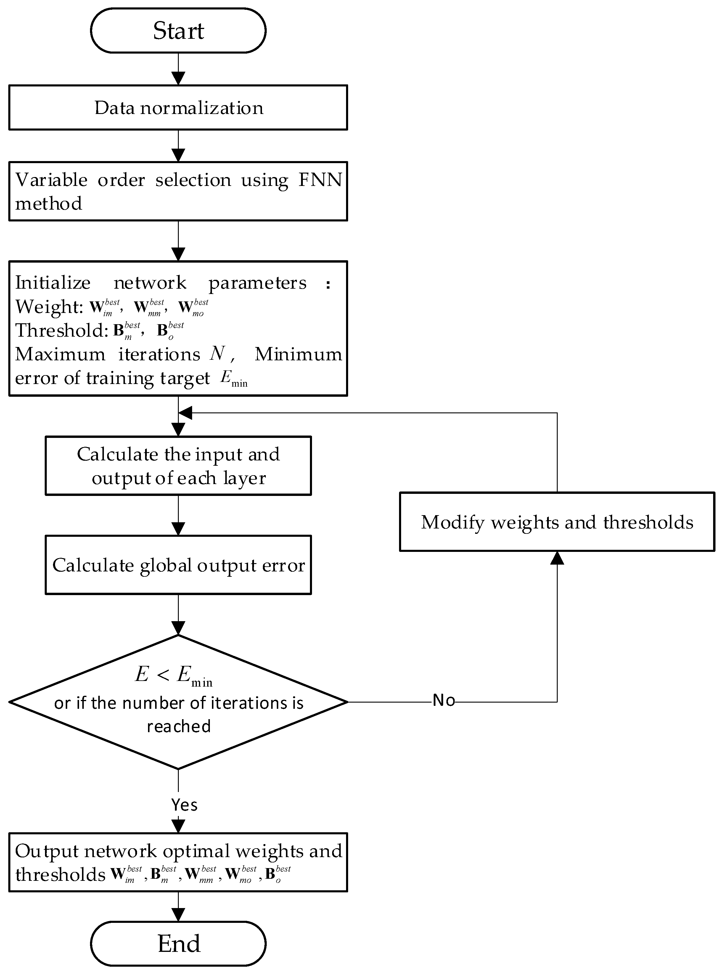
According to the above-mentioned continuous correction of the weight threshold, the global error is calculated, and the training stops when the set error accuracy or the maximum number of iterations is reached. The optimal weight and threshold matrix of the Mach number prediction model are obtained at this time, noted as  W i m b e s t ,   B m b e s t ,   W m m b e s t ,   W m o b e s t ,   B o b e s t . Finally, the output of the prediction model is inversely normalized to obtain the Mach number prediction value  M a p ( k )  for a single operating condition.
In summary, the Mach number NARX-Elman prediction model is established, as shown in Figure 1. The specific establishment process is shown in Figure 2.

2.4. IOSBC-GA Mach Number Migration

Wind tunnel tests are costly and have long construction cycles, and a large number of pretest modeling is required for different conditions, which would be more costly if each condition is first tested completely before building the corresponding model. Therefore, model migration can be achieved if a small amount of new data is used to correct the base model parameters.
Based on the known historical prediction model and a small amount of experimental data for the new condition, the prediction model can be built by migration for the new condition. However, because of the different wind tunnel flow field characteristics in the wind tunnel system according to the set values, the similarity between the historical and new conditions needs to be evaluated before the migration process.

2.4.1. Similarity Analysis among Different Modes

First, the similarity between the old and new working conditions needs to be calculated based on their data characteristics. In this paper, the Euclidean distance method is adopted to assess the similarity between the two sets of working conditions, and the distances between the old and new working condition samples are as follows:
d i C i , C n e w = C i C n e w 2 = k = 1 n c i k c n e w k 2 1 2
where  C i  is the ith historical feature,  C n e w  is the new feature, and n is the number of features set.
For better comparison, this distance is normalized to between 0 and 1 to obtain the similarity:
s i m i C i , C n e w = 1 1 + d i C i , C n e w
The historical working condition with the greatest similarity to the new working condition will be found among all the historical working conditions, and the model based on this historical working condition is used as the base model. Then, a small amount of the new working condition data is used to carry out model migration by the IOSBC method, and the optimal deviation slope correction parameter will be found by the GA optimization algorithm.

2.4.2. Mode Migration Using IOSBC Model

The IOSBC method was first proposed by Gao for the injection molding process [24]. The method treats the new process as a shift and scaling of the historical process, and model migration can be performed under the new process by deviation slope correction, and the relationship between the input and output of two similar working conditions can be corrected using a small amount of data. The method requires a small number of samples, has a low computational effort, and is suitable for model migration for a wide range of operating modes.
In 2012, Jiesheng Wang proposed an adaptive soft sensor modeling method based on wavelet neural network (WNN) in order to predict the key technical indicators of the grinding process (grinding granularity and mill discharge speed), and used a model migration strategy and input-output spatial bias correction (IOSBC) method to achieve online adaptive correction of the soft sensor model, showing the adaptive correction of the process [25]. In 2019, Tao et al. developed a data-driven base model for a superranger engine combustion chamber to complete the prediction of the total pressure of the new combustion chamber by the IOSBC method. The feasibility of the combustion chamber migration strategy was verified by comparing it with the actual process mechanical properties [26]. The principle of the IOSBC model migration method is shown in Figure 3.
The input of the base model represented in Figure 3 is  X 1 , the output is  Y 1 , the base model established is  Y 1 = f ( X 1 ) , and the new model can be obtained by migrating the input and output respectively, where  X 2  is the input of the new model,  Y 2  is the output of the new model.
In this paper, IOSBC method is applied to achieve the following steps:
First, the known input and output data of the new working condition are normalized, and the input data are migrated so that the input variable in the base model after migration is:
r ( k ) = S I r n e w ( k ) + B I
where  S I = [ s 1 , , s n ] T B I = [ b 1 , , b n ] T  are the slope and bias migration coefficient matrices of the model inputs, and n is the number of model input variables.
Then, the optimal weights and threshold matrices of the established model are migrated, and the weights matrix of the input layer to the intermediate layer for the new working condition is defined as  V i m , and the threshold matrix is  C m . The weights matrix of the intermediate layer to the undertaking layer is  V m m , the weights matrix of the intermediate layer to the output layer is  V m o , and the threshold matrix is  C o . Then, the weights and threshold matrices of the new working condition are:
V i m = s 11 × w 11 + b 11 s 1 n × w 1 n + b 1 n s l 1 × w l 1 + b l 1 s l n × w l n + b l n
C m = s 1 × b 1 + b 1 s l × b l + b l T
V m m = s 11 × w 11 + b 11 s l 1 × w l 1 + b l 1 s l 1 × w l 1 + b l 1 s l l × w l l + b l l
V m o = s 11 × w 11 + b 11 s l 1 × w l 1 + b l 1 s q 1 × w q 1 + b q 1 s q l × w q l + b q l
C o = s 1 × b 1 + b 1 s q × b q + b q T
where  s i j , b i j , s i , b i   ( i = 1 l ; j = 1 n )  are the slopes of the weight threshold and the deviation migration coefficients of the input layer to each neuron in the middle layer.  s i i , b i i  are the slopes of the weight threshold and the deviation migration coefficients of the middle layer to each neuron in the succession layer.  s p i , b p i , s p , b p   ( i = 1 l ; p = 1 q )  are the weight threshold slopes and deviation migration coefficients of the intermediate layer to each neuron in the output layer.
The new model after migration can be obtained as:
M a p , n o r ( k ) = f o ( V m o x ( k ) C o )
x ( k ) = f m ( V m m x C ( k ) + V i m ( S I r n e w ( k 1 ) + B I ) C m )
x C ( k ) = x ( k 1 )
The output of the new model prediction is back-normalized to obtain the new model Mach number prediction  M a p n e w .
The optimization parameters in the new model are obtained by optimizing the following equations by bringing in a small amount of known data of the new operating conditions:
arg min J S I , B I , V i m , C m , V m m , V m o , C o = ε ε T ε = M a n e w M a p n e w
where  M a n e w  is the actual output value for the new operating conditions,  J  is the new model after migration.
For solving the optimization equations, most traditional optimization algorithms require the selection of initial values, which, if not chosen properly, can lead to a local optimum, making iterations impossible. Therefore, in this paper, a genetic algorithm independent of the initial value is chosen to optimize the equation and find the global optimal solution. The algorithm has strong robustness and can be independent of the solution domain.

2.4.3. Parameter Optimization Using Genetic Algorithm

Genetic algorithms are also known as evolutionary algorithms [27], and the main idea is borrowed from Darwin’s model of evolution under natural selection. By drawing on evolutionary theory, genetic algorithms model the problem to be solved as a biological evolutionary process, finding the optimal solution to the task through continuous evolution. The main processes include population individual setting, population coding, decoding, crossover, variation, selection algorithms, and fitness functions. It can be summarized as a random selection of individuals in a limited range, selection based on the fitness of each individual, retention of individuals with high fitness, elimination of individuals with low fitness, and updating until the optimal result is approached.
In this paper, the reciprocal of the sum of squared errors between the true value of Mach number,  M a n e w , known for the new working condition, and the predicted value of Mach number  M a p n e w  for the new model is chosen as the fitness function of the genetic algorithm:
F i t = 1 ( M a n e w M a p n e w )
When the evolutionary algebra meets the termination evolutionary algebra or reaches the minimum set error, the calculation is stopped, and the optimal solution of the model migration coefficients are obtained at this time, which are denoted as  S I b e s t ,   B I b e s t ,   V i m b e s t ,   V m m b e s t ,   C m b e s t ,   V m o b e s t ,   C o b e s t , respectively. Finally, the output of the prediction model will be processed by inverse normalization to obtain the predicted Mach number for the new working condition.

3. Illustration and Discussion

3.1. Experimental Conditions and Settings

3.1.1. Continuous Wind Tunnel Blowing System Pneumatic Structure

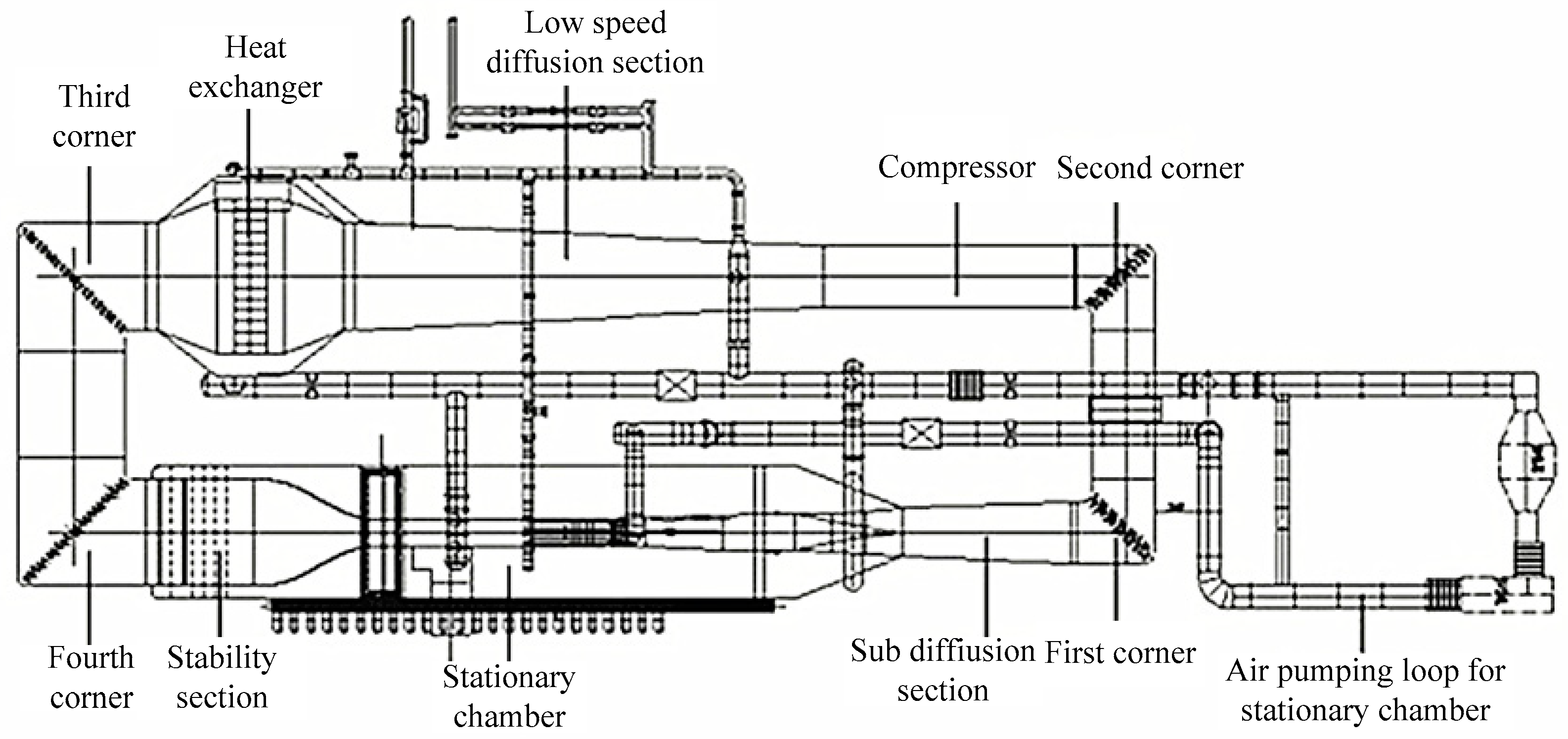
The wind tunnel shown in Figure 4 is a typical continuous transonic wind tunnel, using dry air as the test medium and adopting a new technical solution of high-performance heat exchanger and adjustable central body to improve the wind tunnel’s smooth quality and operation efficiency. The total length of the wind tunnel is 26.42 m, and the test section size reaches 0.6 m × 0.6 m × 2.7 m (height × width × length), the wind tunnel temperature range is 233~333 K, the total design pressure range is 0.02~0.4 MPa, the test section Mach number range is 0.3~1.5, the rated power of the main compressor can reach 5000 KW, the rated power of the auxiliary compressor reaches 1500 KW. The body of the wind tunnel is made entirely of steel, mainly consisting of four corners, cooling section, compressor, and test section.
The design of the tunnel in the figure uses many technical elements to improve the flow field quality and operational efficiency. When the wind tunnel is ready, all main exhaust valves are closed, and the main regulator is opened to quickly create the wind tunnel flow field.
As the wind tunnel runs over time, the total air pressure in the stabilization section reaches its target value through the action of the controller. At this moment, high-pressure gas enters the tunnel from a storage tank all the time. In order to better stabilize the flow field, the main venting valve starts to work and, through the action of the controller, the gas is evacuated over time so that the total gas pressure in the stabilized section is stabilized around the target value. After a period, the static pressure in the test section also reached the target value. Then the Mach number is stabilized at the experimentally specified value. Finally, the experimental data were obtained after the attitude of the vehicle model changed according to the predetermined rules and the wind tunnel flow field returned to the set conditions.

3.1.2. Continuous Wind Tunnel Blowing Test Process

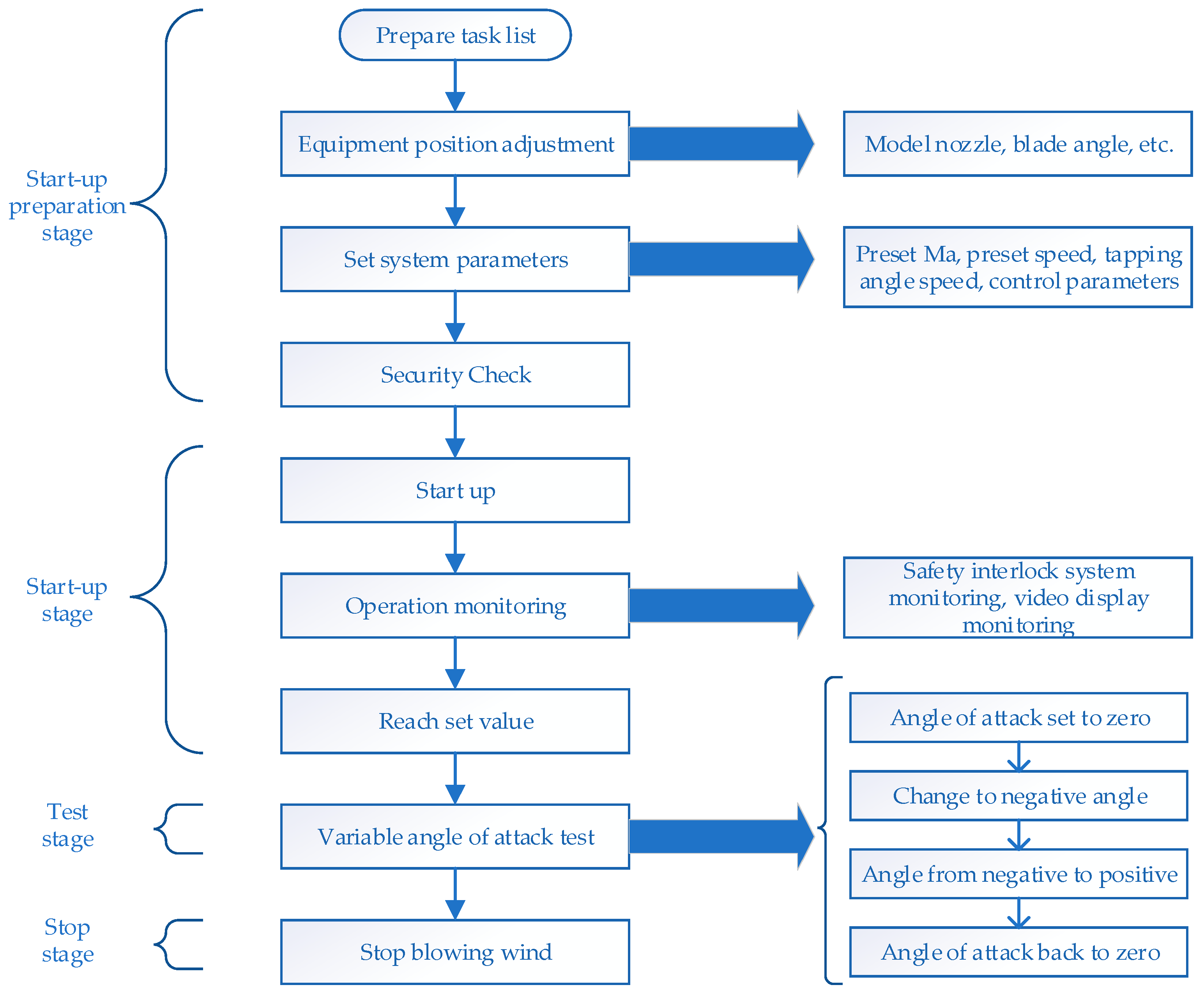
In continuous wind tunnel, there is also a serious coupling phenomenon between the total pressure and Mach number. If the total pressure needs to be changed, the medium-pressure air supply system needs to be used to replenish the gas or pump out the gas inside the wind tunnel, and the pressure perturbation will adversely affect the Mach number control during the inflation or pumping process. Likewise, the total pressure is constantly changing during the Mach number control with the rotational speed. After the wind tunnel test is started, the system is first brought up to the preset Mach number through the total pressure regulation and the control of compressor speed, and then the variable angle of attack test is started, which is changed according to the set speed and change range. The change of the angle will lead to a huge disturbance of the wind-driven flow field and make the Mach number exceed the control accuracy requirement. In this case, it is necessary to adjust the compressor speed while changing the angle of attack to make the Mach number stable within a certain accuracy range. By running the above process, the data acquisition work is carried out. After completion, the angle of attack is returned to zero, and the vehicle is shut down, leaving the wind tunnel in its initial state and ready for the next test. The overall blowing process can be divided into the start-up preparation stage, start-up operation stage, test stage, and stop stage. The detailed flow chart of the wind tunnel blowing process is shown in Figure 5.

3.1.3. Analysis of Variables and Selection of Working Conditions for the Modeling Process

Before the test of the wind tunnel, many parameters need to be set. First, the Mach number needs to be set for the current operating conditions. Different Mach number settings lead to different gas flow rates in the wind tunnel so changes in the angle of attack of the model have different effects on the Mach number, and the system characteristics change. For the selection of total pressure, atmospheric pressure is the most common operating pressure, and its total pressure setting value is 100 Kpa which is also the pressure state in which the most number of tests are conducted in the wind tunnel system. In addition, the wind tunnel is also equipped with conditions such as the blade angle, pilot slit, and opening/closing ratio, and the difference of these conditions will also lead to the change of flow field characteristics and generate new working conditions. Moreover, the different change rates of the angle of attack have different effects on the Mach number. In the continuous variable angle of attack test, the greater the change speed of the angle of attack, the greater the perturbation on the Mach number.
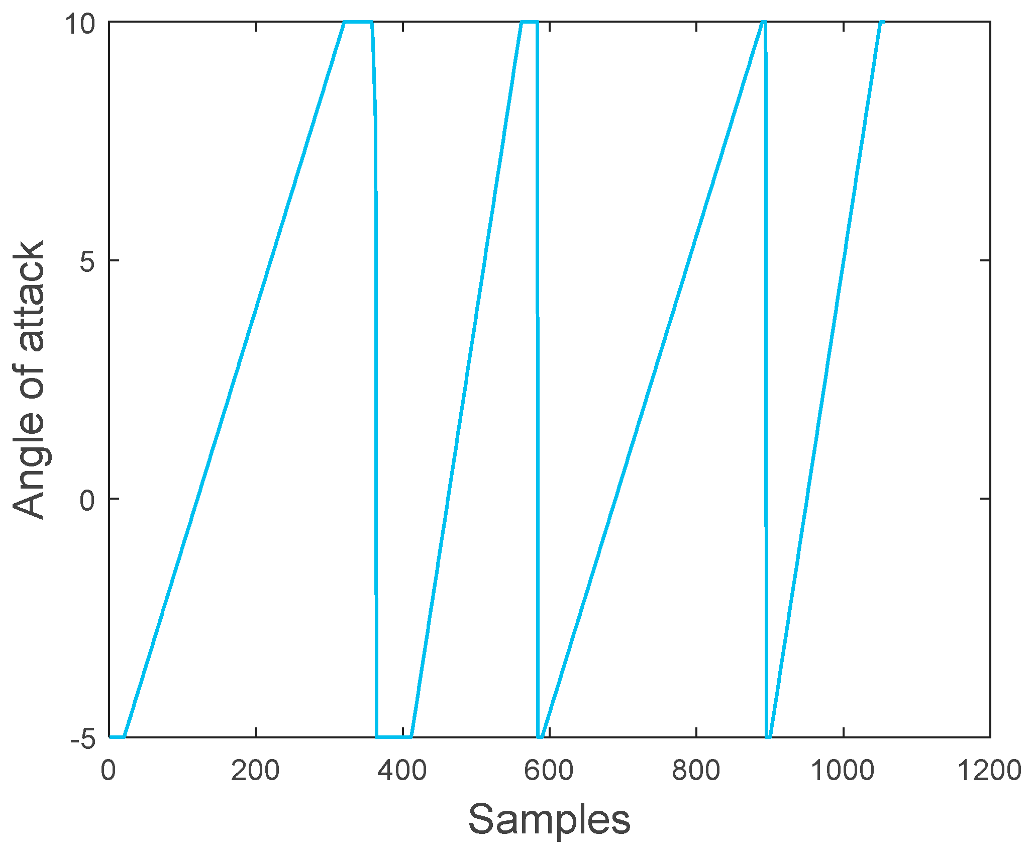
In this paper, three working conditions with sufficient data accumulation are selected as typical working conditions, and the real-time Mach numbers of the working conditions are between 0.8 and 0.9 in the transonic velocity range, in which the lead slit is set to 24 mm. The opening/closing ratio is set to 1.5%, the total pressure is set to 100 Kpa at atmospheric pressure, the blade angle is 76.5° and 56.3°, and the angle of attack change speed is 0.1°/s and 0.2°/s. The continuous variable angle of attack can change the angle of attack in a wide range, and at the same time, the speed of the angle of attack change can be changed, which is fast in operation, efficient, and cost-saving. The work in this paper focuses on the continuous variable angle of attack case, and the angle of attack change curve from −5° to −10° is shown in Figure 6.
The working conditions are set as shown in Table 1.

3.2. Mach Number Prediction for a Single Mode

In this paper, two conditions are selected, working condition 1 (Mach number 0.85) and working condition 2 (Mach number 0.9). Firstly, the order of each variable is determined by FNN, and order analysis for all the variables is carried out in all the test conditions. It is found that the order of each variable is slightly different in different conditions. In order to better select the order to show its applicability, and avoid the instability of single test results, and make the test closer to the real situation, the average value of each variable in the order analysis under different working conditions is selected as the order of the final model, i.e., the best variable order, as shown in Table 2.
In summary, the FNN algorithm is used to determine the variable orders  n P 0 n s n A n , and  n M a , which can be 4, 5, 6, and 5, respectively, so that the variable information can be included comprehensively and without redundancy.
Make the sum of the best order of variables found above as the number of neurons in the input layer of NARX-Elman model, denoted as n = 20. Since only the Mach number is used as the output, the number of neurons in the output layer is recorded as q = 1. The number of neurons in the middle layer is calculated according to the common empirical Formula (29), and in this paper  α  is taken as 5 to obtain the number of middle neurons l = 10.
l = n + q + α
The initial weights and thresholds in the model work are randomly given, and the rest parameters are adjusted after many experimental runs and parameters. Finally, the model setting parameters are selected: the maximum training number is 1000, the minimum error of the training target is 0.001, In the wind tunnel flow field control, the momentum factor is in the range of 0.5~0.99, and the learning rate is in the range of 0.001~0.8. For the model developed in this paper, the momentum factor is 0.9, and the learning rate is 0.005. 70% of the data of each test condition are selected for training, and 30% of the data are tested.
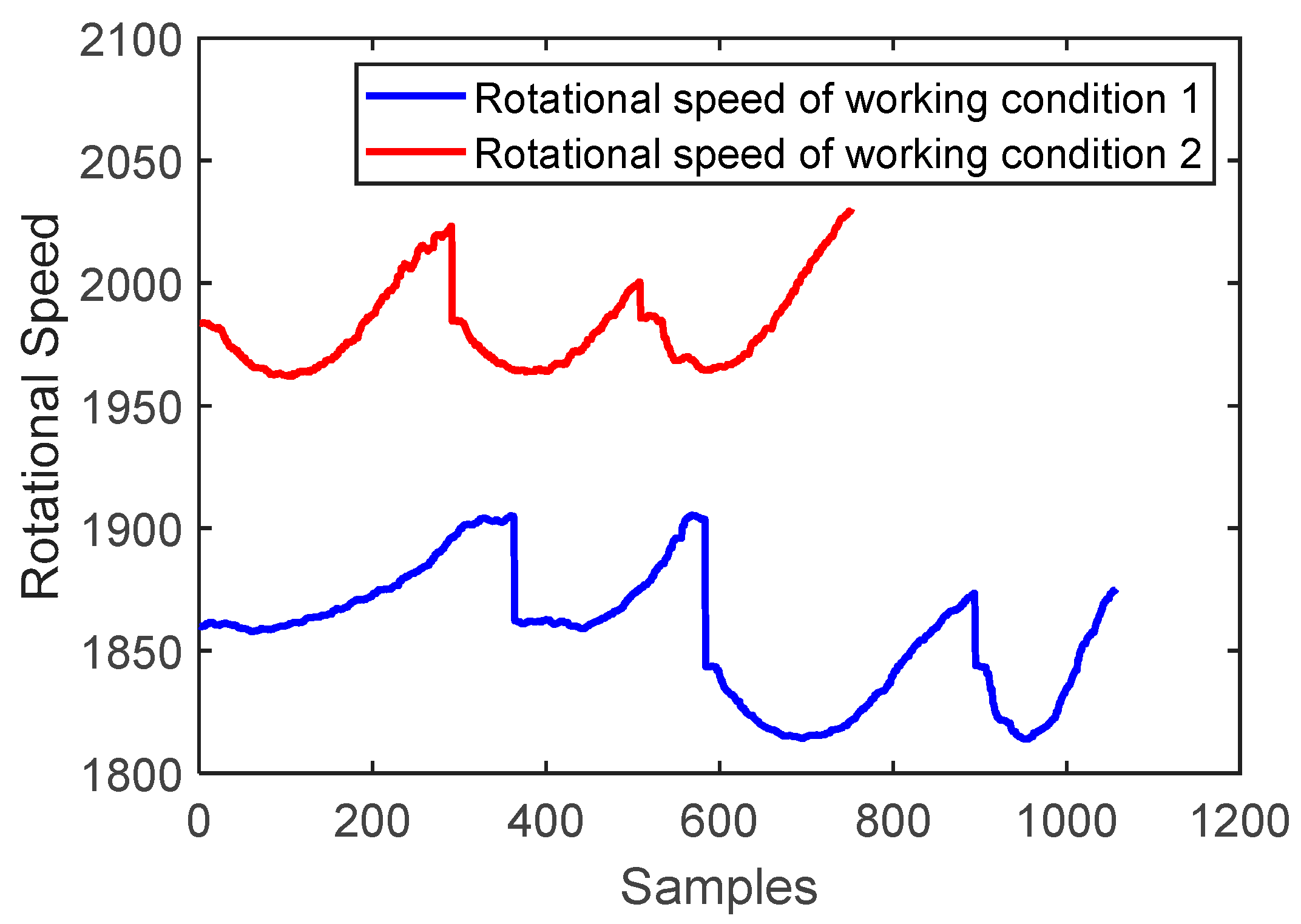
Analysis of the input control variables for working condition 1 and working condition 2, the controlled Mach number angle of attack variation for this test varies continuously between −5° and 10°, as shown in Figure 6, and the total pressure variation and speed variation at different Mach numbers for the two tests are shown in Figure 7 and Figure 8.
The continuous variable angle of attack variation in working condition 1 and working condition 2 are similar, as shown in Figure 6, and the variation of the angle of attack in the test is discussed in this paper with working condition 1 as an example. There are 1057 data points in working condition 1, of which 143 data points are in the region of constant angle of attack, −5° to 10°, and the remaining 914 data points are in the region of the transient mode of the angle of attack, as shown in Figure 9.
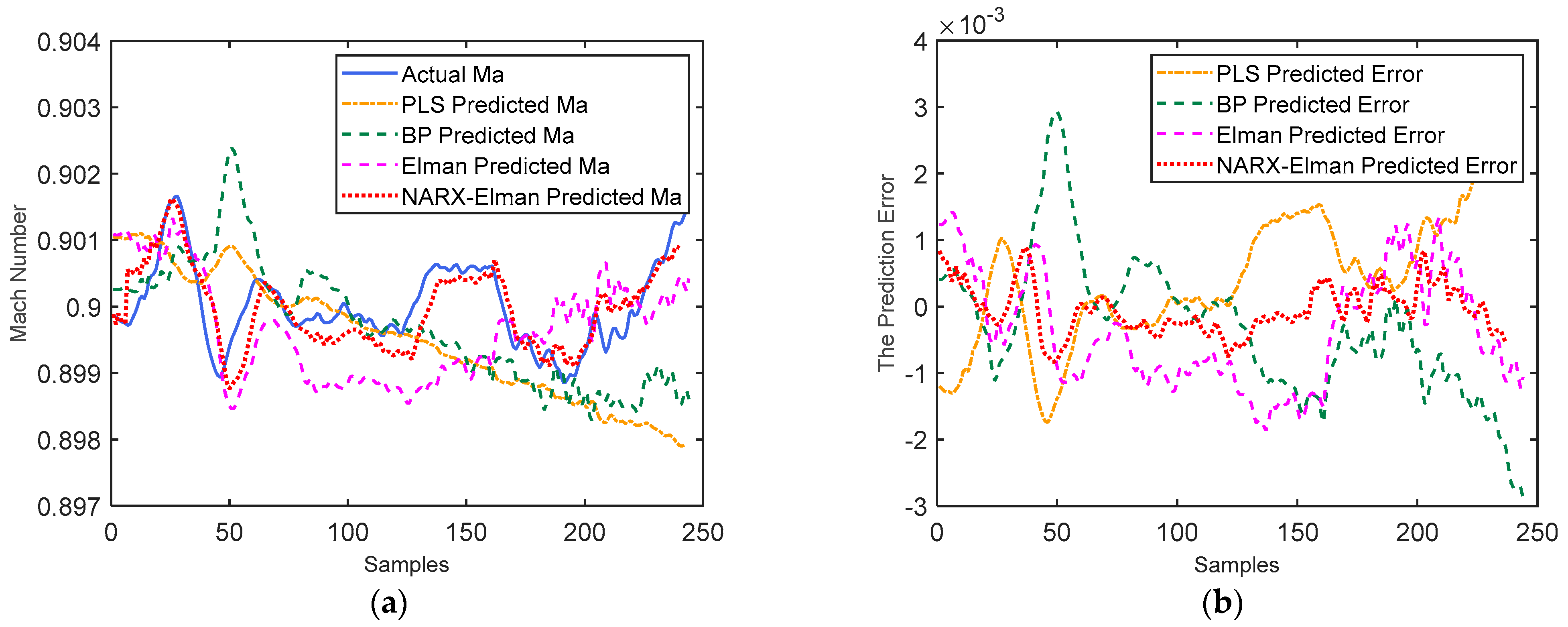
Mach number prediction is performed using the NARX-Elman model, and the results are compared with those of the traditional model PLS regression prediction model, BP neural network model, and Elman neural network model, as shown in Figure 10 and Figure 11.
The data in Figure 10 and Figure 11 each show the continuous variation of Mach number predictions in one test, corresponding to a sequence of measurements, respectively. According to the graphs of Mach number prediction results and Mach number prediction errors of the three models mentioned above, the trend of Mach number variation predicted by using the NARX-Elman model is closer to the actual Mach number, compared to the PLS method, BP neural network prediction method, and Elman neural network prediction method, which predict the trends of Mach number variation that are more different from the actual Mach number. The established prediction models are evaluated with three model evaluation indexes to further illustrate the superiority of the NARX-Elman model, as shown in Table 3 and Table 4 for working condition 1 and working condition 2, respectively.
First, the root mean square error (RMSE) is selected to evaluate the four models built for two separate operating conditions. The RMSE value is a measure of the deviation between the predicted and true values, and its smaller value indicates that the predicted value is closer to the true value. The RMSE value is required to be less than 0.001 in practice, and the formula is shown below:
RMSE = 1 K k = 1 K M a ( k ) M a p ( k ) 2
The RMSE values of the Elman model and the NARX-Elman model are less than 0.001, and the RMSE values predicted by the NARX-Elman model are 0.00016 and 0.00037, respectively, which are much smaller than the accuracy of the other three models, indicating that the model proposed in this paper can achieve high prediction accuracy.
Secondly, considering that the evaluation of the model should consider not only the accuracy of the prediction but also the impact on the control effect, two indexes, Mach number accuracy (A) and maximum deviation (MD), are selected in this paper to evaluate the control effect of the model. A is the deviation between the set value and the average predicted value in the prediction process. The smaller the Mach number accuracy, the better the model reflects the overall change of the Mach number.
A = M a s e t 1 K k = 1 K M a p ( k )
where  M a s e t  is the Mach number setting value.
From the model prediction results under working condition 1 and working condition 2, it can be obtained that the A values of PLS, BP, and Elman models are close to each other, while NARX-Elman yields A of 0.00001 and 0.00002, respectively, which is one order of magnitude smaller than the remaining three models. The results show that the overall value of the Mach number predicted by the model proposed in this paper has a minimal deviation from the preset value and a small deviation from the overall change case.
The maximum deviation (MD) is the maximum prediction deviation between the actual value and the predicted value throughout the prediction process. It reflects whether the stability of the Mach number can meet the requirements, and the project requires that the maximum deviation of the Mach number does not exceed 0.001.
M D = max M a ( k ) M a p ( k )
Comparing the maximum deviations obtained from the predictions of the four models, the MD values of the remaining three models are greater than 0.001, while the MD value of the NARX-Elman model proposed in this paper is 0.00089 under both operating conditions, which is less than 0.001 and meets the control accuracy requirements.
In summary, the error between the predicted Mach number and the actual Mach number of the NARX-Elman model proposed in this paper is closer to 0. The Mach number prediction accuracy and control effect are better than those of the PLS method, BP neural network method, and Elman method.
After obtaining the high-performance and high-precision NARX-Elman model, the Mach number prediction model established by the single working condition is applied to the control simulation system to analyze the feasibility of the model as a controller for predictive control so as to accurately control the Mach number of the wind tunnel flow field. In the simulation control system, the accuracy of the model can be obtained at less than 0.001, which has validity and effectiveness, and further control and next theoretical research can be carried out under the real wind tunnel test.

3.3. Mach Number Prediction for Multiple Modes

According to the similarity analysis and migration method, working condition 3 is selected as the new working condition for migration, and according to the results calculated by the similarity, the similarity between working condition 1 and the new working condition is obtained as 0.7011, and the similarity between working condition 2 and the new working condition is 0.7110, so the first 10% of the test data of the new working condition are selected as known data, and the rest of the data are used as test data for migration of the two base models. To illustrate the superiority of the migration model, a separate NARX-Elman model is built as a non-migration model using the 10% of data known for the new working condition, and the prediction results are compared with those of the migration model. The set parameters in the genetic algorithm are adjusted through several experiments, and the final selected parameters are shown in Table 5.
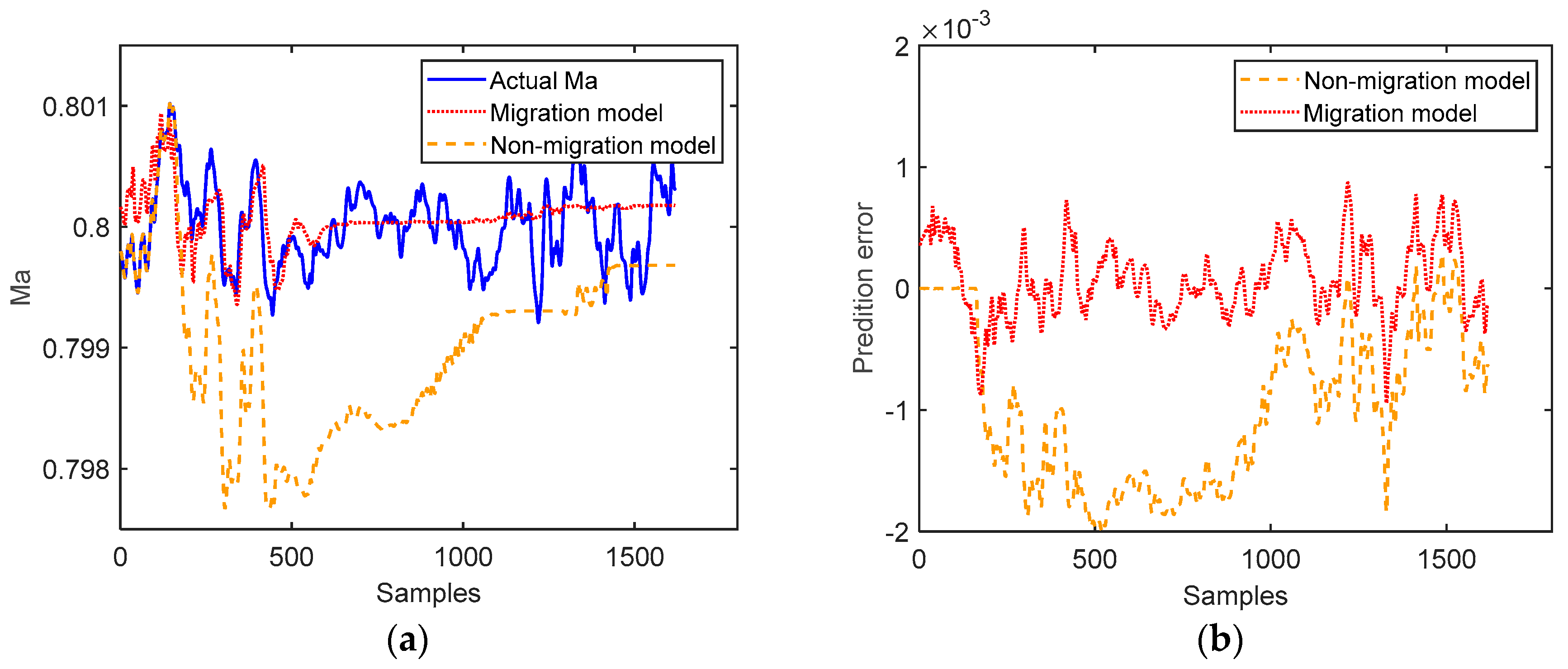
When working condition 1 is selected as the base model and 10% of the data before the new working condition are modeled and migrated for optimization, the resulting fitness curves are shown in Figure 12, and the Mach number prediction results and prediction errors for the non-migrated and migrated models are shown in Figure 13.
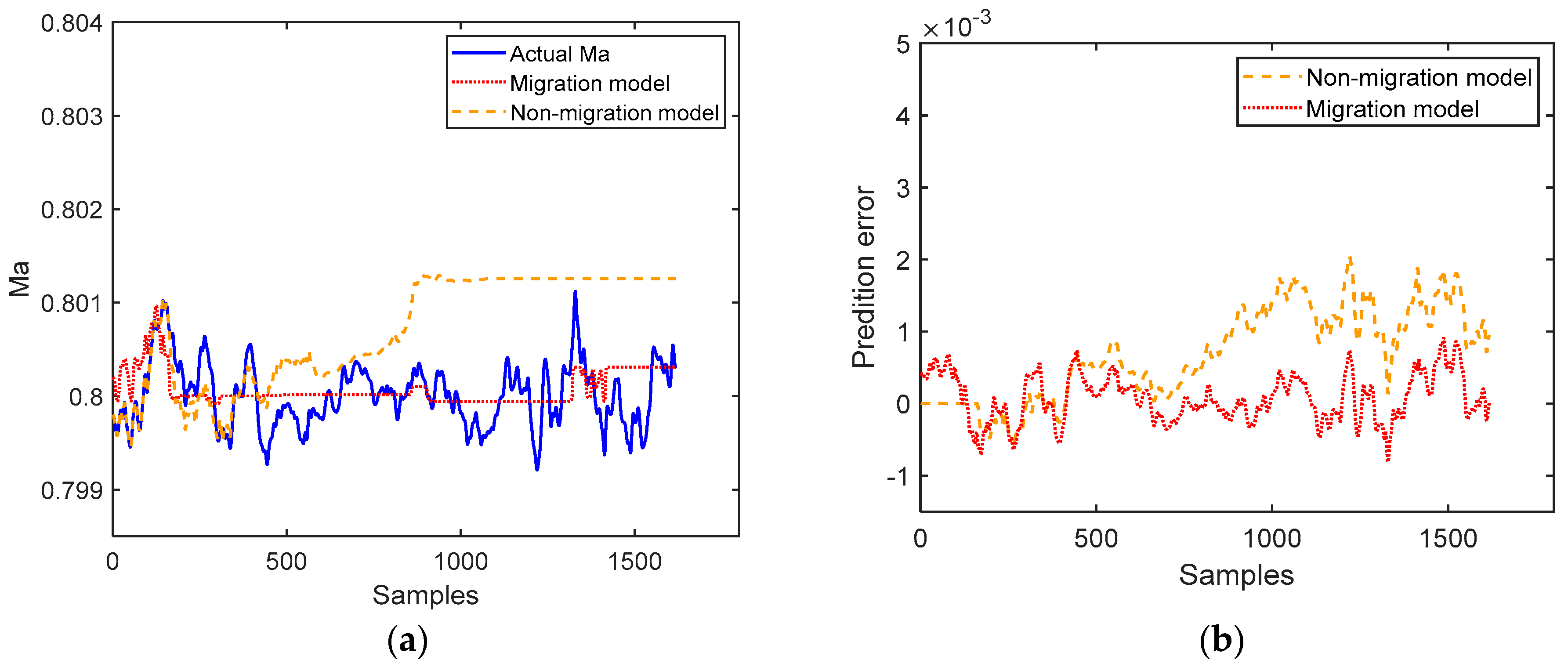
When working condition 2 is selected as the base model and 10% of the data before the new working condition are modeled and migrated for optimization, the resulting adaptation curves are shown in Figure 14, and the prediction results and prediction errors of Mach number for the non-migrated and migrated models are shown in Figure 15.
From Figure 13 and Figure 15, it can be concluded that the Mach number predicted by the migration model is closer to the actual Mach number when the amount of new modal data is small. According to the Mach number prediction error analysis, the error of the Mach number predicted by the migration model is closer to 0, and the prediction error is smaller than the prediction error of the non-migration model.
The model evaluation indexes of the above non-migration model and migration model are compared, and the specific data indexes are shown in Table 6.
The analysis of Table 6 shows that the non-migration model predicts the Mach number with RMSE greater than 0.001 under the base model with working conditions of 1 and 2. For the migration model, the Mach number prediction RMSE is within 0.001 under the base model with working conditions of 1 and 2. Meanwhile, the maximum deviation MD and A of Mach number prediction for the migration model prediction are much smaller than those of the non-migration model under both models, and the RMSE and MD values are both less than 0.001, which meets the required prediction accuracy. Therefore, the results show that the migration model approach has better prediction effects with fewer data.

4. Conclusions

In this paper, firstly, a NARX-Elman Mach number prediction model is proposed, where the NARX model is adopted as the model structure, using the FNN algorithm to determine the order of the input variables and using the dynamic Elman neural network as the nonlinear fitting function of the NARX model. Secondly, a migration model based on the IOSBC-GA method is proposed, using the IOSBC method with the characteristic of low requirements for data as the mapping relationship between the base model and the new model. Then combining a small amount of data from the new working condition, the GA algorithm is used to find the slope of deviation in the new model so as to correct the relationship of the input and output in the base model and establish a Mach number prediction model for the new working conditions. Finally, when the prediction models established with the NARX-Elman method are used to predict the Mach number of two operating conditions online, the proposed method resulted in a higher prediction accuracy compared with the four conventional methods. Comparing the migrated model with the model established without migration, the evaluation results of the migrated model are much smaller than those of the non-migrated model, which verifies the effectiveness of the proposed method.
The NARX-Elman model proposed in this paper is a novel modeling method based on a dynamic neural network model for predictive control. It has higher control accuracy and stability compared with traditional control methods and can have wider applicability in practical applications. The ideas proposed in the model in this paper are based on a stable and reliable mathematical theory, with certain theoretical support and reliability guarantee, which can be used as an extension and improvement of other predictive control methods and lead the technological innovation and development of related fields.

Author Contributions

Conceptualization, L.Z.; methodology, L.Z., Y.S. and W.J.; software, Y.S.; validation, Y.S. and W.J.; formal analysis, Y.S.; investigation, L.Z.; resources, L.Z.; data curation, L.Z.; writing–original draft preparation, Y.S.; writing—review and editing, Y.S.; visualization, Y.S.; supervision, L.Z.; project administration, L.Z.; funding acquisition, L.Z. All authors have read and agreed to the published version of the manuscript.

Funding

This research was funded by the National Natural Science Foundation of China (No. 61503069) and the Fundamental Research Funds for the Central Universities (N150404020).

Data Availability Statement

All data used during the study were provided by a third party. Direct requests for data may be made to the provider as indicated in the Acknowledgements.

Acknowledgments

All data were provided by Aviation Technology Key Laboratory of Aerodynamics Research in High-Speed and High Reynolds.

Conflicts of Interest

The authors declare no conflict of interest.

References

  1. Desai, S.S. Relative roles of computational fluid dynamics and wind tunnel testing in the development of aircraft. Curr. Sci. 2003, 84, 49–64. [Google Scholar]
  2. Haley, P.; Soloway, D. Generalized predictive control for active flutter suppression. IEEE Control Syst. Mag. 1997, 17, 64–70. [Google Scholar] [CrossRef]
  3. Shahrbabaki, A.N.; Bazazzadeh, M.; Manshadi, M.D.; Shahriari, A. Designing a fuzzy logic controller for the Reynolds number in a blowdown supersonic wind tunnel. In Proceedings of the 2014 IEEE Aerospace Conference, Big Sky, MT, USA, 3–10 March 2014. [Google Scholar]
  4. Luo, Y.; Xing, S.; Song, W.; Chen, T.; Gao, Q. Fuzzy and PID compound control of Mach number for 0.6 meters supersonic wind tunnel. In Proceedings of the 2011 2nd International Conference on Artificial Intelligence, Management Science and Electronic Commerce (AIMSEC), Dengleng, China, 8–10 August 2011. [Google Scholar]
  5. Guo, J.; Zhang, R.; Cui, X.; Huang, X.; Zhao, L. Mach number prediction and analysis of multi-mode wind tunnel system. In Proceedings of the 2020 Chinese Automation Congress (CAC), Shanghai, China, 6–8 November 2020; pp. 6895–6900. [Google Scholar]
  6. Zhang, T.; Mao, Z.; Yuan, P. Decoupled PID controller for wind tunnel system. In Proceedings of the 26th Chinese Control and Decision Conference (2014 CCDC), Changsha, China, 31 May–2 June 2014; pp. 3547–3550. [Google Scholar]
  7. Ng, W.F.; Popernack, T.G. Combination probe for hi-frequency unsteady aerodynamic measurements. IEEE Trans. Aerosp. Electron. Syst. 1988, 24, 76–84. [Google Scholar] [CrossRef]
  8. Tang, Y.; Li, H.; Cai, Y. State space description based predictive control for normal temperature continuous transonic wind tunnel. In Proceedings of the 2016 Chinese Control and Decision Conference (CCDC), Yinchuan, China, 28–30 May 2016. [Google Scholar]
  9. Zhang, J.; Yuan, P.; Chin, K. Model predictive control for the flow field in an intermittent transonic wind tunnel. IEEE Trans. Aerosp. Electron. Syst. 2017, 54, 324–338. [Google Scholar] [CrossRef]
  10. Triplett, W.E. Wind tunnel correlation study of aerodynamic modeling for F/A-18 wing-store tip-missile flutter. J. Aircr. 1984, 21, 329–334. [Google Scholar] [CrossRef]
  11. Müller, D.; Reichert, M.; Herbst, J. Data-driven modeling and coordination of large process structures. In Proceedings of the Move to Meaningful Internet Systems 2007: CoopIS, DOA, ODBASE, GADA, and IS: OTM Confederated International Conferences CoopIS, DOA, ODBASE, GADA, and IS 2007, Vilamoura, Portugal, 25–30 November 2007; Proceedings, Part I. Springer: Berlin/Heidelberg, Germany, 2007; pp. 131–149. [Google Scholar]
  12. Mark, A.; Jose, C.P. Classification and prediction of wind tunnel Mach number responses using both competitive and gamma neural networks. Assoc. Comput. Mach. 2007, 1, 252–260. [Google Scholar]
  13. Tang, X.; Liu, K.; Wang, X.; Gao, F.; Macro, J.; Widanage, W.D. Model migration neural network for predicting battery aging trajectories. IEEE Trans. Transp. Electrif. 2020, 6, 363–374. [Google Scholar] [CrossRef]
  14. Park, J.; Lee, S.Y.; Choi, L.Y.; Jeong, H.; Noh, H.H.; Yu, S.H.; Song, H.; Hong, S.W. Analyzing drift patterns of spray booms with different nozzle types and working pressures in wind tunnel. J. Korean Soc. Agric. Eng. 2021, 63, 39–47. [Google Scholar]
  15. Li, Z.; Qin, Y.; Hou, S.; Zhang, R.; Sun, H. Renewable energy system based on IFOA-BP neural network load forecast. Energy Rep. 2020, 6, 1585–1590. [Google Scholar] [CrossRef]
  16. Huang, M.; Hong, C.; Chen, J.; Ma, C.; Li, C.; Huang, Y. Prediction of peak shear strength of rock joints based on back-propagation neural network. Int. J. Geomech. 2021, 21, 04021085. [Google Scholar] [CrossRef]
  17. Elman, J.L. Finding structure in time. Cogn. Sci. 1990, 14, 179–211. [Google Scholar] [CrossRef]
  18. Leontaritis, I.; Billings, S. Input-output parametric models for non-linear systems part I: Deterministic non-linear systems. Int. J. Control 1985, 41, 303–328. [Google Scholar] [CrossRef]
  19. Leontaritis, I.; Billings, S. Input-output parametric models for non-linear systems part II: Stochastic non-linear systems. Int. J. Control 1985, 41, 329–344. [Google Scholar] [CrossRef]
  20. Mohd, N.; Aziz, N. Performance and robustness evaluation of Nonlinear Autoregressive with Exogenous input model predictive control in controlling industrial fermentation process. J. Clean. Prod. 2016, 136, 42–50. [Google Scholar] [CrossRef]
  21. Broomhead, D.; King, P. Extracting qualitative dynamics from experimental data. Phys. D Nonlinear Phenom. 1986, 20, 217–236. [Google Scholar] [CrossRef]
  22. Mathew, B.K.; Brown, R. Determing embedding dimension for phase-space reconstruction using a geometrical construction. Phys. Rev. A 1992, 45, 3403–3411. [Google Scholar]
  23. Aksamit, N.; Whitfield, P. Examining the pluvial to nival river regime spectrum using nonlinear methods: Minimum delay embedding dimension. J. Hydrol. 2019, 572, 851–868. [Google Scholar] [CrossRef]
  24. Lu, J.; Gao, F. Process modeling based on process similarity. Ind. Eng. Chem. Res. 2008, 47, 1967–1974. [Google Scholar] [CrossRef]
  25. Wang, J.; Yang, Y.; Sun, S. SFLA-WNN Soft-Sensor Modeling and Reconfiguration of Grinding Process Based on Model Migration. J. Shanghai Jiaotong Univ. 2012, 46, 1951–1955. [Google Scholar]
  26. Tang, C.; Yang, O. Modeling of scramjet combustors based on model migration and process similarity. Energies 2019, 12, 2516. [Google Scholar]
  27. Holland, J. Genetic algorithms. Sci. Am. 1992, 267, 66–73. [Google Scholar] [CrossRef]
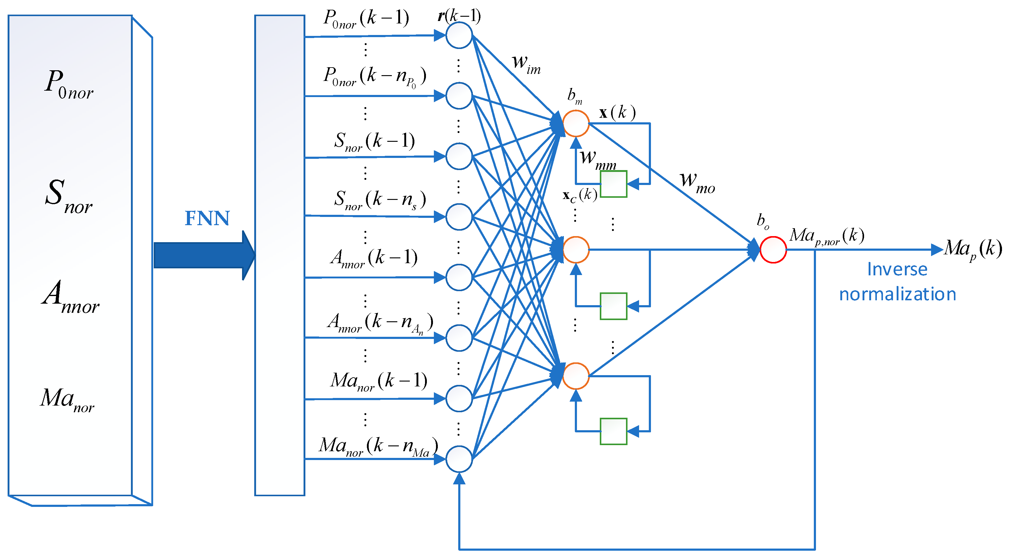
Figure 1. NARX-Elman prediction model of the Mach number.
Aerospace 10 00498 g001
Figure 2. Flow chart of the Mach number NARX-Elman model design.
Aerospace 10 00498 g002
Figure 3. Schematic diagram of IOSBC model migration.
Aerospace 10 00498 g003
Figure 4. Structural diagram of a continuous transonic wind tunnel.
Aerospace 10 00498 g004
Figure 5. Blowing process of the wind tunnel.
Aerospace 10 00498 g005
Figure 6. Continuous change curve of the angle of attack.
Aerospace 10 00498 g006
Figure 7. Rotational speed of working condition 1 and 2.
Aerospace 10 00498 g007
Figure 8. Total pressure of working condition 1 and 2.
Aerospace 10 00498 g008
Figure 9. Variation of the angle of attack in the test of working condition 1.
Aerospace 10 00498 g009
Figure 10. (a) Prediction curves and (b) error curves of Mach number under working condition 1.
Aerospace 10 00498 g010
Figure 11. (a) Prediction curves and (b) error curves of Mach number under working condition 2.
Aerospace 10 00498 g011
Figure 12. Genetic algorithm adaptation curve with working condition 1 as the base model.
Aerospace 10 00498 g012
Figure 13. (a) Prediction curves and (b) error curves of Mach number for the new working condition, with working condition 1 as the base model.
Aerospace 10 00498 g013
Figure 14. Genetic algorithm adaptation curve with working condition 2 as the base model.
Aerospace 10 00498 g014
Figure 15. (a) Prediction curves and (b) error curves of Mach number for the new working condition, with working condition 2 as the base model.
Aerospace 10 00498 g015
Table 1. Working conditions of the wind tunnel flow field.
Test
Conditions
Ma   P 0 Blade Angle (°)   A n Total Sample
10.8510056.30.11057
20.9010076.50.2752
30.8010076.50.11626
Table 2. Optimal order of variables.
VariablesTotal PressureRotational SpeedAngle of AttackMach Number
Best Order4565
Table 3. Evaluation indexes of Mach number prediction for the model built in working condition 1.
PLSBP
RMSEAMDRMSEAMD
0.00130.00110.00270.00080.00030.0027
ElmanNARX-Elman
RMSEAMDRMSEAMD
0.00060.00020.00240.000160.000010.00089
Table 4. Evaluation indexes of Mach number prediction for the model built in working condition 2.
PLSBP
RMSEAMDRMSEAMD
0.00120.00040.00360.00110.00030.0029
ElmanNARX-Elman
RMSEAMDRMSEAMD
0.00090.00030.00190.000370.000020.00089
Table 5. Setting of GA algorithm parameters.
ParameterValue
Number of groups80
Termination of evolutionary algebra100
Crossover probability0.6
Mutation probability0.01
Table 6. Mach number prediction evaluation indexes of non-migration model and migration model.
Base Working
Condition
Non-Migration ModelMigration Model
RMSEAMDRMSEAMD
10.001200.000980.002000.000320.000080.00094
20.001300.000410.002700.000340.000080.00092
Disclaimer/Publisher’s Note: The statements, opinions and data contained in all publications are solely those of the individual author(s) and contributor(s) and not of MDPI and/or the editor(s). MDPI and/or the editor(s) disclaim responsibility for any injury to people or property resulting from any ideas, methods, instructions or products referred to in the content.