Thrust Prediction of Aircraft Engine Enabled by Fusing Domain Knowledge and Neural Network Model

Abstract

Accurate prediction of aircraft engine thrust is crucial for engine health management (EHM), which seeks to improve the safety and reliability of aircraft propulsion. Thrust prediction is implemented using an on-board adaptive model for EHM. However, the conventional methods for building such a model are often tedious or overly data-dependent. To improve the accuracy of thrust prediction, domain knowledge can be leveraged. Hence, this study presents a strategy for building an on-board adaptive model that can predict aircraft engine thrust in real-time. The strategy combines engine knowledge and neural network architecture to construct a prediction model. The whole-model architecture is divided into separate modules that are mapped in a one-to-one form using a domain decomposition approach. The engine domain knowledge is used to guide feature selection and the neural network architecture design in the method. Furthermore, this study explains the relationships between aircraft engine features and how the model can predict engine thrust in flight condition. To demonstrate the effectiveness and robustness of the architecture, four different testing datasets were used for validation. The results show that the thrust prediction model created by the given architecture has maximum relative deviations below 4.0% and average relative deviations below 2.0% on all testing datasets. In comparison to the performance of the models created by conventional neural network architecture on the four testing datasets, the model created by the presented architecture proves more suitable for aircraft propulsion.

1. Introduction

As a complex system with high-reliability requirements, aircraft engines are developed with engine health management (EHM) to increase reliability [1]. With the advancements in avionics, research focused on EHM is developing from off-board to on-board [2]. Compared to the off-board EHM, on-board EHM enables real-time continuous engine performance monitoring [3]. One important task in on-board EHM is building an on-board adaptive model to predict the engine performance, specifically thrust [4].

In general, an on-board adaptive model consists of an on-board real-time model and a modifier [5]. The on-board real-time model is typically a linearized model based on an aerothermodynamics-based component-level model of engine [6]. Currently, the Kalman filter [7] is commonly used, and effective methods for correcting the results are predicted by an on-board real-time model. Many improvements to the Kalman filter were given [8,9,10] to increase the accuracy of parameter prediction. Further, the e-storm model for parameter estimation was presented based on the Kalman filter method by NASA [11]. A novel linear parameter-varying approach was made for thrust estimation [12], and developing an on-board adaptive model is still attractive. It is remarkable that on-board real-time model accuracy is crucial for the on-board adaptive model. However, complex objecting modeling such as aircraft engines require conditional assumption and can suffer from errors caused by modeling methods and model solving, decreasing the model accuracy [13,14]. For aircraft engines, the strong coupling in the engine systems and the degradation of engine performance is difficult to be represented by the high-precision physical model.

On the other hand, data-driven methods have been developed for an on-board adaptive model for predicting engine parameters [15,16]. Data-driven methods discard physical equations and obtain information from data. Through sufficient representative data, data-driven methods use mathematics to find a model or a combination of models that approximate the exact physical model. Four typical data-driven methods, including Random Forest (RF), Generalized Regression Neural Network (GRNN), Support Vector Regression (SVR), and Radial Basis Neural Network (RBNs) have been used to develop a temperature baseline model for aircraft engine performance health management [17]. Zhao et al. performed much research on support vector machines (SVMs) and used SVMs for aircraft engine parameter estimation [18]. Zhao studied other methods for thrust prediction, such as radial basis networks [19]. An extreme learning machine is also used in aircraft engine parameter estimation [20]. However, the quality and quantity of data greatly affect the final result in a data-driven method. Relying solely on the data without physical constraints may produce an unreasonable result in data-driven methods [21].

To address the issue that the accuracy of the data-driven method model is limited by the training dataset, hybrid methods that incorporate physical information have been developed [22,23]. Reference [24] describes three methods for adding physical information to neural networks (a kind of data-driven method), namely observational biases, inductive biases, and learning biases. Observational biases add data that reflect underlying physical principles to the neural network. For example, data augmentation techniques [25] such as rotating, zooming, flipping, and shifting an image can create additional data that reflect physical invariance. Inductive bias is how to tailor a neural network architecture to satisfy a set of physical functions; for example, a node in a neural network can represents a physical symbol, and the connection between the nodes can satisfy the operator in a physical function [26,27]. Learning biases can be introduced by the intervening training phase of a data-driven model, and the training of a model converges towards a solution that adheres to underlying physical constraints. One way to introduce learning biases is by imposing physical equations or principles to penalize the loss function of conventional neural networks [28,29]. The above-mentioned methods for the hybrid model relate to differential or algebraic equations. However, due to the complexity of the physical equations related to aircraft engine systems, these methods for an on-board model may be challenging to implement in the short term.

To avoid the complexity of dealing with mathematical physical equations, the focus of this study was to explore the combination of aircraft engine knowledge and the neural network models. In this study, an on-board adaptive model for predicting engine thrust is given by blending engine domain knowledge and the neural network models. In Section 2, the architecture of the hybrid model is presented in detail, which fuses networks for predicting engine parameters. The section also provides a brief introduction to the traditional neural network model. Additionally, the relationships between aircraft engine features are described to explain why the model trained with ground measurable data can be used in the flight condition. Next, a model for predicting engine thrust based on the architecture is discussed. In Section 3, the models are verified using simulation data and compared with conventional neural network models. Finally, Section 4 concludes the study.

2. On-Board Adaptive Model

2.1. Architecture by Fusing Physical Structure and Neural Network

Inspired by the integration of coupling relationships between engine components (such as Figure 1a), the domain decomposition approach is used to deconstruct the neural network structure. In the digital space, a large neural network is divided into multiple independent neural networks, corresponding to engine components in the physical space. The coupling relationships guide the interconnection of independent neural networks in the digital space. The architecture integrates neural networks and aircraft engine domain knowledge using the following points:

• Based on domain decomposition, a neural network is divided into multiple subnetworks and the number of which corresponds to the number of engine components.
• A subnetwork represents an engine component, and the input features of the subnetwork are related to the corresponding engine component.
• The subnetworks are interconnected based on the interconnection between the engine components. The order of data flowing through the subnetwork is based on the order in which air flows through the engine component. For example, the air flows sequentially through an inlet, a fan, and then a compressor. Correspondingly, the data flow sequentially through an inlet subnetwork, a fan subnetwork, and then a compressor subnetwork.
• The physical constraint on the networks is that the rotation speed of the components on the same axial is equal. For example, the same rotation speed is used as input to a fan subnetwork and a low-pressure turbine subnetwork.

Specifically, the architecture consists of three layers that make up the neural networks. The first layer is the component/system learning layer, the second layer is referred to as the coupling layer, and the last layer is the mapping layer, as shown in Figure 1b. Each layer performs its function. The component/system learning layer processes the input features based on the coupling relationships of the engine components. The coupling layer integrates features according to the operation order of the engine components. The mapping layer is a regressive analysis that connects abstract features with target parameters.

The component/system learning layer comprises multiple independent neural networks, each of which represents an engine component or system and is referred to as a component/system learning network. A sequence of component learning networks forms the main body of the component/system learning layer. The networks are arranged in the order of components located in the engine main flow. A component network reads features from two parts: sensor parameters that measure the corresponding component and the feature from a component network in the same shaft. For example, the inlet network reads the total pressure at the inlet entry, and the high-pressure turbine network reads the corresponding component feature and the feature from the compressor network. The combustor network receives the fuel flow rate as input, and the turbine network reads the temperature and pressure measured at the component section. Thus, the physical constraint that components working on the same shaft have an equal rotation speed is mapped to the digital space. A system learning network, such as an oil system network or a control system network, also reads the corresponding parameters to learn the system characteristics. The position of a system network is determined by the role of the corresponding system in the engine. Therefore, the number of component/system learning networks equals the number of engine components/systems. After processing the measured variables, the component/system learning layer outputs the abstract features as input to the coupling layer. The role of the coupling layer is to learn the relation between components/systems and extract a coupling feature from the discrete features of component/system networks. Like the sequence in which air flows through engine components, the data transmission in the coupling layer follows this order. Finally, the mapping layer associates the feature from the coupling layer with the aircraft engine performance parameter.

From the above description, it can be seen that the presented architecture serves as a designing framework for a predicting model and it is not limited to a particular engine type. Compared to conventional neural networks, incorporating coupling relationships of engine components into neural networks simplifies feature selection. The input features are filtered and clustered based on the requirements of the component/system networks. Moreover, the presented architecture does not mandate all input features to be input at once. Instead, a component/system learning network only reads relevant sensor parameters, thereby reducing the need for network nodes and avoiding direct processing of unrelated input features.

2.2. Component Network

The component networks play a crucial role in the training of presented architecture. One of the simplest methods for component network is to use the mature artificial neural network (ANN) [30], such as a fully connected neural network (FNN), recurrent neural networks (RNNs), convolutional neural networks (CNNs), etc. The neural network model consists of stacked neural networks, where the network is made up of nodes that store information. Nodes receive input data and distribute independent weights for each output. Figure 2 illustrates the standard mode of node connection. In a fully connected neural network, the connections between nodes are unidirectional and only exist from one layer to the next layer. As such, a fully connected neural network focuses on extracting features from single data but ignores the relationship between the data in space or time. To address this issue, recurrent neural networks were introduced. RNN is an ANN with a self-circulating structure composed of nodes participating in recursive computations, which is called a cell in terminology. The cell transfers information from the previous calculation to the following calculation, thereby improving the performance on sequence data. However, long-term dependence issues such as information morphing and vanishing may occur when vanilla RNN processes overtime sequences. Long short-term memory (LSTM) neural network was introduced to handle long-term dependence [31].

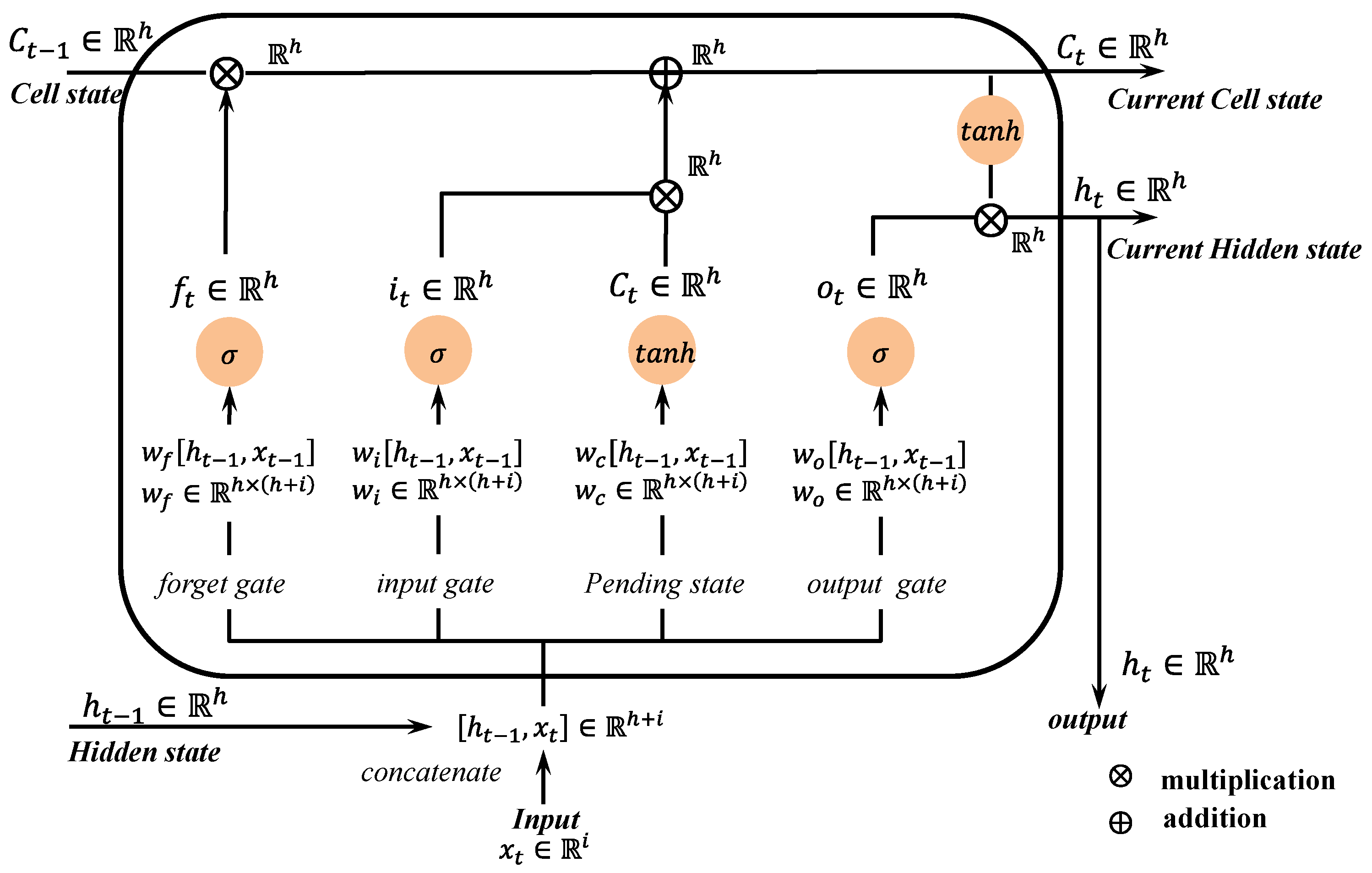
An LSTM network is a kind of RNN with a gate function. There are three gate functions in an LSTM cell: input gates, forget gates, and output gates. The input gate controls how much input information is transmitted. The forget gate selects a part of the information in the previous sequence to be discarded according to the input data. Selecting appropriate information for the following sequence is the output gate function. The three gate formulas are as follows:

$$f_t=\sigma \left(W_f\left[h_{t-1}, x_t\right]+b_f\right)$$

(1)

$$i_t=\sigma \left(W_i\left[h_{t-1}, x_t\right]+b_i\right)$$

(2)

$${\overline{C}}_t=\tanh \left(W_{{}_c}\left[h_{t-1}, x_t\right]+b_c\right)$$

(3)

$$C_t=f_t\otimes C_{t-1}+i_t\otimes {\overline{C}}_t$$

(4)

$$O_t=\sigma \left(W_o\left[h_{t-1}, x_t\right]+b_o\right)$$

(5)

$$h_t=O_t\otimes \tanh \left(C_t\right)$$

(6)

where b represents the bias; W represents the learnable weights of the nodes; x represents the input features; h represents the hidden state of the LSTM cell that is the cell output features; subscript t represents the number of cells; subscript f represents the forget gate parameters; subscript i represents the input gate parameters, and subscript o represents the output gate parameters. $\otimes$ represents the tensor product. $\sigma$ is a sigmoid function that produces a result range of 0 to 1. The information flow process of an LSTM cell is shown in Figure 3. Generally, gradient descent algorithms are the common methods used for training artificial neural networks. More details about training algorithms are available in references [32,33,34] and are not included in detail.

In some cases, it may be useful to analyze the input features in the reverse order of the input sequence. In such cases, a bidirectional LSTM (Bi-LSTM) can be employed. A bidirectional LSTM network is a composite structure of two LSTM networks with the same cell, where one LSTM network processes the input data in the original order of the input sequence, and the other processes the same input data in the reverse order of the input sequence. The outputs of the two LSTM networks are combined into one as the final network output.

2.3. Model for Predicting Thrust

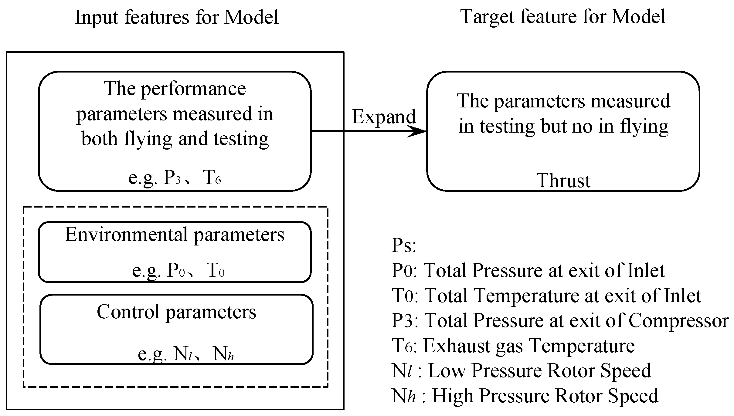
Based on the presented architecture, a model for predicting thrust was built. Firstly, the parameters for model training were discussed. The model training is supervised learning where the input data and the corresponding output data are provided to the model during the training phase. For the on-board model, the training phase of the model is typically completed in a ground system, while the usage of the model takes place on the airborne system. Thus, the selection of input features for the model is limited, as both the ground system and airborne system must be capable of measuring the selected features. Thrust is associated with the aircraft engine status, control law, and engine operating environment. Consequently, the parameters related to the condition are selected as input features. The relationship between the component performance parameters and the aircraft engine performance parameters reflects the physical matching of components and the entire engine. The model represents the physical matching when these parameters are used to train the model as input and target features. Thus, the thrust data collected from engine testing, including ground and high-altitude tests, can be training data for a thrust prediction model. In this way, it is equivalent to expand the number of measurable parameters on the airborne system. The relationship between the parameters is shown in Figure 4.

Next, the specific neural network used in the architecture layer for the prediction model is discussed. For example, the independent component/system networks and the mapping layer use a fully connected neural network in the prediction model, while the coupling layer uses a bidirectional LSTM. Since the order of engine components is sequenced in space, LSTM is prioritized to complete the coupling layer. An LSTM reads and analyses the input features in the forward order of the sequence. For an aircraft engine, the rear component affects the front component when an adverse pressure gradient occurs in the engine. Therefore, a bidirectional LSTM is selected for the coupling layer.

According to the above description, Algorithm 1 outlines the steps involved in developing a thrust prediction model based on the presented architecture.

Algorithm 1 The hybrid architecture-based thrust prediction model
1	Determine the number of component networks according to the aircraft engine type.
2	Connect the component network to build the component learning layer.
3	The component networks are arranged in the order in which air flows through the components in the engine.
4	The output of component networks points to the coupling layer;
	The output of the coupling layer points to the mapping layer;
	The output of the mapping layer is a target parameter.
5	Determine the neural network type for each layer:
	Component learning layer (component network): FNN;
	Coupling layer: Bi-LSTM;
	Mapping layer: FNN.
6	Measurable parameters are classified by component correlation;
	Measurable parameters are the input for component network, thrust as the target.
7	Preprocess data with the Min–Max normalization method.
8	Set the batch size and the node number of the network; choose MSE as the loss
	function and RMSE for optimization.
9	Training model:
	For i = 1 to iter:
	Tune the weight value of the model to minimize the loss function.
	End

3. Verification and Discussion

3.1. Case Settings

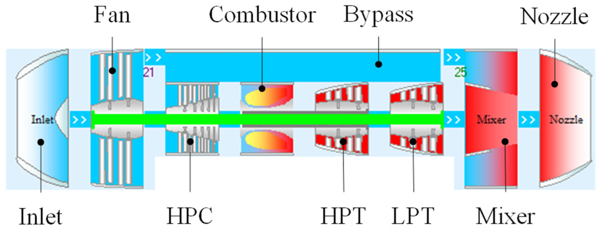
The dataset used to verify the given method was collected from the performance simulation of a two-spool mixing exhaust turbofan. The engine performance simulation utilized component-level modeling where the thermodynamic cycle in each component is simulated using a given component characteristic map. Figure 5 shows a sketch of the component-level model of the engine, which includes an inlet, a fan, a high-pressure compressor (HPC), a combustor, a high-pressure turbine (HPT), a low-pressure turbine (LPT), a mixing chamber, a bypass, and a nozzle.

The engine performance simulation generated five datasets; one is the training dataset and four are testing datasets. The component characteristic maps used to generate these datasets are different. High-pressure components work in harsh environments and have a faster decay rate than other engine components. Thus, different combinations of component characteristic maps were created to account for varying degrees of degradation in high-pressure components. The four testing datasets are named Testing 1, 2-1, 2-2, and 2-3. There are four combinations of the component characteristic maps: Maps A, Maps B, Maps C, and Maps D. Maps B, C, and D were generated by multiplying the correction factor based on Maps A, where the correction coefficient ranged from 0.7 to 0.99. Maps A were used to generate the training dataset and Testing 1, while Maps B, C, D were used to generate Testing 2-1, Testing 2-2, and Testing 2-3, respectively. Therefore, the training dataset and Testing 1 simulate an aircraft engine state without performance degradation, while Testing 2 simulates aircraft engine states with varying degrees of performance degradation.

The training dataset characterizes the entire operation of an engine from start to stop. To include as many engine states as possible, the training dataset has 10,001 samples. Testing 1 has 40,044 samples and characterizes engine operation under four different control laws, compared to the training dataset. Testing 2 has 10,001 samples and is used to verify model accuracy under engine degradation state.

The features for model training are clustered based on Section 2.3, as presented in

Table 1. The input features for the predicting model.

Type of Parameter	Cross-Section of Component/ Acronym	Component Network
Total temperature/K	Outlet of inlet/T0	Inlet network
	Outlet of fan/T25	Fan network
	Exhaust gas temperature/T6	LP turbine network
Total pressure/kPa	Outlet of inlet/P0	Inlet network
	Outlet of fan/P25	Fan network
	Outlet of compressor/P3	Compressor network
Control/controlled parameter	Low-pressure rotor speed/Nl	Fan network
		LP turbine network
	High-pressure rotor speed/Nh	Compressor network
		HP turbine network
	Fuel flow rate/Wf	Combustor network
Aircraft engine performance parameter	Thrust/Fn	Target parameter

. Since the selected features have difference magnitudes, they are normalized using Min–Max normalization. To evaluate the effectiveness of the presented architecture, multiple thrust predicting models are developed based on the conventional neural network architecture (Figure 6a), simplified block neural network architecture (Figure 6b), and hybrid neural network architecture (Figure 6c). The number of nodes in the predicting models is close to the training sample size. To prevent overfitting, a dropout layer with a 0.3 drop rate is added before the mapping layer in every predicting model based on the number of training samples.

Table 2. The configuration of the thrust predicting model.

Model Name	Architecture	First Layer	Second Layer	Other Layers	The Total Number of Nodes
AN-1	Conventional	FC (100)	FC (100)	\	11,201
AN-2	Conventional	FC (100)	FC (60)	FC (60)	10,781
AN-3	Conventional	FC (100)	FC (50)	FC (50)-FC (40)	10,681
Str-1	Simple block	BiL (4)	BiL (32)	\	11,713
Str-2	Simple block	FC (50)-FC (4)	BiL (32)	\	11,513
Str-3	Simple block	FC (100)	BiL (30)	Lambda	10,101
Str-4	Simple block	BiL (2)	BiL (32)	\	9821
Str-5	Hybrid	FC (4)	BiL (32)	\	10,149
Str-6	Hybrid	FC (8)	BiL (32)	\	10,313
Str-7	Hybrid	FC (4)	BiL (48)	\	13,857
LS-1	Conventional	BiL (12)	BiL (24)	Sequence Length (9)	11,569

presents the configuration of the predicting models. The models AN-1, AN-2, AN-3, and LS-1 are developed based on the conventional neural network architecture. The models Str-1, Str-2, Str-3, and Str-4 are developed based on the simple block architecture. The models Str-5, Str-6, and Str-7 are developed based on the hybrid neural network architecture.

For a model developed with conventional architecture, all input features are combined into a vector and fed into the model. In contrast, a model developed using the other two architectures, input features are grouped into multiple vectors. The input and output layers for each model are shown in Figure 7. In Table 2, FC represents the fully connected neural network layer, while BiL represents the bidirectional long short-term memory network layer. The value in parentheses indicates the hyperparameter of the network layer. For example, AN-3 model has four fully connected neural network layers stacked, and the output nodes of each layer are 100, 50, 50, and 40, respectively. For models developed using the simple block architecture or hybrid neural network architecture, the configuration of the first layer network column in Table 2 pertains to each substructure in the first layer of the model, i.e., the network block structure or component network. For instance, in the Str-5 model, all component networks (the inlet network, the fan network, the compressor network, etc.) are fully connected neural network layers with five output nodes.

3.2. Performance Metric

A scoring indicator, namely the root mean squared error (RMSE), was used to measure the loss in a training process and is denoted e_rms(i). The RMSE is defined as follows:

$$e_{rms}(i)=\frac{1}{N}{{\displaystyle \sum _{i=1}^N(Y_{\mathrm{i}}-{\widehat{Y}}_i)}}^2$$

(7)

The maximum relative deviation (MRD) and the average relative deviation (ARD) were chosen as the evaluation indices to evaluate the performance of the presented model:

$$R{D}_i=\left|\frac{V_p-V_t}{V_t}\right|, i=1, 2,\dots , N$$

(8)

$$MRD=\max (R{D}_i, i=1, 2,\dots , N)$$

(9)

$$ARD=\frac{1}{N}{\displaystyle \sum _{i=1}^N(R{D}_i)}$$

(10)

where N represents the number of instances in the testing dataset, V_p and V_t denote the predictive value and the test data, respectively, and the values are divided by the maximum value of the dataset. RD_j is the relative deviation of the instance of the jth testing dataset, MRD denotes the maximum relative deviation of the testing dataset, and ARD denotes the average relative deviation of the testing dataset.

3.3. Results and Discussion

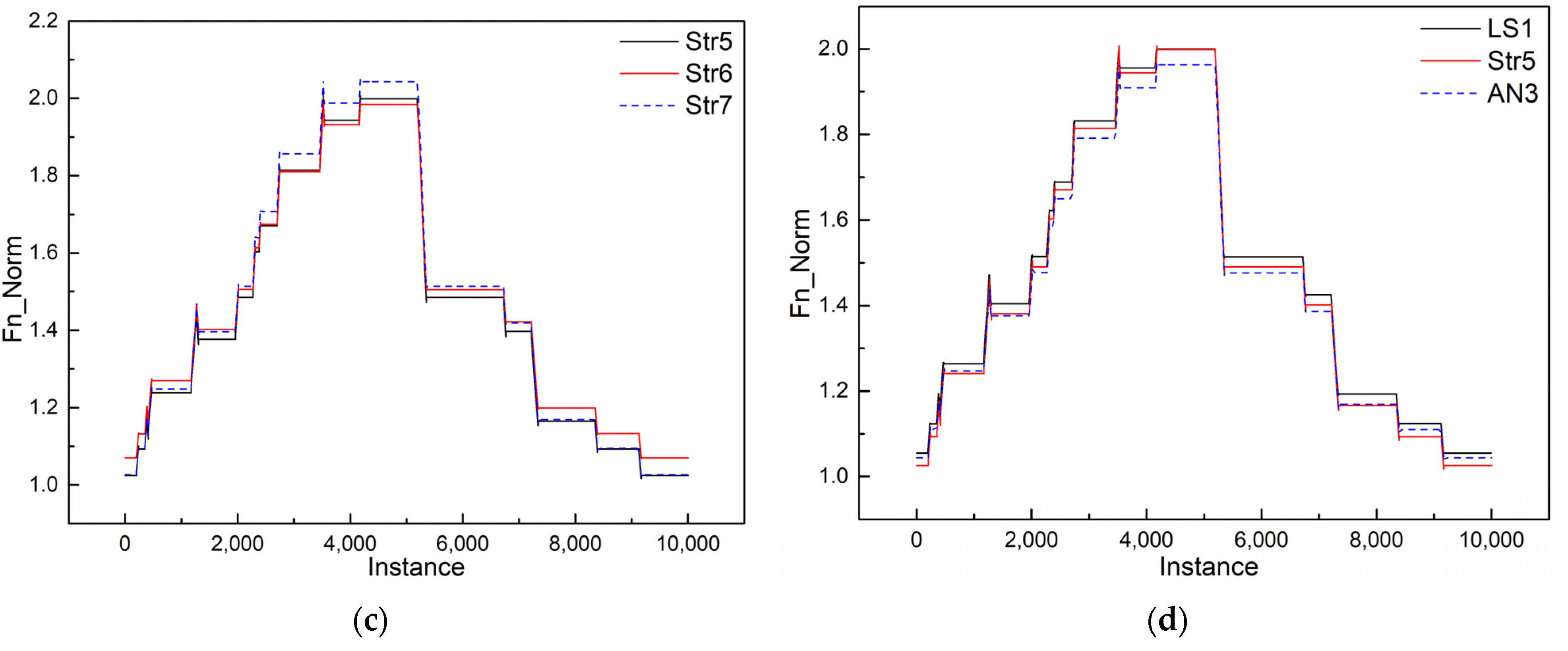
Each model is trained five times using a training dataset to reduce the randomness of the training process. The maximum value, minimum value, mean value, and standard deviation of ARD and MRD for the five results are computed and rounded up to four decimal places. The results of the models on the four testing datasets are presented in

Table 3. Results of the thrust predicting models on the testing datasets 1.

Model	ARD				MRD
	Max %	Min %	Std.	Mean %	Max %	Min %	Std.	Mean %
Testing Dataset 1
AN-1	1.3633	0.3610	0.0048	0.7324	2.3970	1.0077	0.0065	1.5453
AN-2	1.332	0.2609	0.0045	0.8602	3.3842	0.7831	0.0101	2.1747
AN-3	2.3639	0.8563	0.0068	1.534	6.0953	2.0993	0.0166	3.3400
Str-1	2.0158	0.2241	0.0070	1.3764	3.8817	0.5153	0.0149	2.7367
Str-2	2.9108	0.4683	0.0098	1.2643	4.0064	1.2529	0.0117	2.4521
Str-3	1.2415	0.3763	0.0035	0.6599	2.0010	1.0146	0.0037	1.4305
Str-4	2.5134	0.2215	0.0101	1.4086	4.0629	0.7235	0.0133	2.6834
Str-5	1.6190	0.2531	0.0053	0.8957	2.8639	0.7364	0.0092	2.0084
Str-6	2.6263	0.5867	0.0081	1.9309	5.0158	1.2956	0.0139	3.3564
Str-7	2.0936	0.0780	0.0054	1.3602	3.4931	1.7716	0.0067	2.6448
LS-1	1.2987	0.3633	0.0042	0.9355	31.642	29.221	0.0117	30.407
Testing Dataset 2-1
AN-1	3.7842	2.6882	0.0045	3.3160	7.7096	6.0131	0.0071	6.9651
AN-2	2.9477	1.0322	0.0078	2.3805	6.9304	2.7426	0.0164	5.3353
AN-3	4.2153	2.1237	0.0095	3.1021	10.203	5.1283	0.1871	7.1988
Str-1	5.4999	1.2474	0.0168	2.6325	7.8605	2.2850	0.0223	4.9320
Str-2	4.5492	0.2893	0.0172	2.5289	7.2269	1.3958	0.0250	4.6247
Str-3	3.1393	1.2299	0.0076	2.0684	6.9090	2.7207	0.0157	4.9956
Str-4	2.5373	0.6163	0.0090	1.5616	6.0721	1.6456	0.0183	3.9637
Str-5	2.2245	0.8123	0.0055	1.3605	5.4286	1.8546	0.0137	3.3643
Str-6	3.6926	0.6533	0.0154	2.0156	8.0805	1.8475	0.0305	4.7318
Str-7	3.6972	1.4409	0.0101	2.3213	4.8455	3.2047	0.0071	4.1794
LS-1	4.0474	1.6943	0.00916	2.8629	8.0474	4.1085	0.0145	6.1554

and

Table 4. Results of the thrust predicting models on the testing datasets 2.

Model	ARD				MRD
	Max %	Min %	Std.	Mean %	Max %	Min %	Std.	Mean %
Testing Dataset 2-2
AN-1	3.8091	2.7000	0.0044	3.3428	7.6944	6.0316	0.0070	6.9876
AN-2	3.0014	1.0153	0.0081	2.4119	6.9846	2.8165	0.0162	5.5582
AN-3	4.2774	2.1498	0.0096	3.1463	10.229	5.1809	0.0186	7.2430
Str-1	5.5318	1.2685	0.0168	2.6604	7.8891	2.3098	0.0224	4.9705
Str-2	4.6903	0.3445	0.0171	2.6489	7.2254	1.2766	0.0252	4.7164
Str-3	3.1902	1.3591	0.0075	2.1474	6.9461	2.8543	0.0154	5.0725
Str-4	2.8107	0.5281	0.0130	1.6001	6.3564	1.5174	0.0196	4.0076
Str-5	2.4076	0.8850	0.0063	1.4650	5.6173	1.9695	0.0143	3.4874
Str-6	3.7327	0.6196	0.0154	2.0597	8.1307	1.9709	0.0301	4.8170
Str-7	3.7408	1.3976	0.0103	2.3859	4.9623	3.1957	0.0075	4.2571
LS-1	4.0642	1.7461	0.0090	2.8997	8.0599	4.1571	0.0143	6.1853
Testing Dataset 2-3
AN-1	3.9344	2.8795	0.0042	3.5255	7.8176	6.1732	0.0069	7.1332
AN-2	3.1761	1.0413	0.0087	2.5571	7.1321	2.9314	0.0163	5.7190
AN-3	4.4586	2.3525	0.0095	3.3026	10.287	5.2857	0.0183	7.3590
Str-1	5.7983	1.4903	0.0172	2.8747	8.1181	2.4377	0.0229	5.1395
Str-2	4.8208	0.0449	0.0171	2.7945	7.2504	1.4033	0.0246	4.8515
Str-3	3.4819	1.5350	0.0079	2.3974	7.1504	2.9540	0.0158	5.2498
Str-4	3.1511	0.3398	0.0118	1.7532	6.5569	1.4514	0.0194	4.2091
Str-5	2.5754	0.8158	0.0072	1.5926	5.7334	2.0804	0.0146	3.5879
Str-6	3.8069	0.6172	0.0155	2.1314	8.1673	2.0353	0.0301	4.8812
Str-7	3.8111	1.3497	0.0106	2.4564	5.0550	3.1940	0.0078	4.3224
LS-1	4.3430	1.9969	0.0091	3.1685	8.2561	4.3434	0.0144	6.3692

. The trends of the model prediction results on the four testing datasets are depicted in Figure 8. Figure 9 displays a histogram of the average MRD of the predicting models on the four testing datasets. Notably, the performance of LS-1 model on Testing 1 differs greatly from the other models, and its result is not shown in Figure 9a. For ease of discussion, the models generated with the conventional architecture are collectively referred to as the conventional models, while the other models are collectively referred to as the structural models.

Table 3 shows that all models have small ARDs. Furthermore, the maximum and minimum values of MRD are mostly below 5% for Testing 1. Not all the structural models perform better than the conventional models on Testing 1. Since the component characteristic maps used in the performance simulation to generate Testing 1 are identical to the training dataset, a model performing well on Testing 1 may rely on the training data. Thus, it is more important to evaluate the performance of the models on the testing dataset that differs from the training data if the model accuracy is met. Additionally, the results of conventional models indicate that increasing the depth or complexity of the model layer does not necessarily improve the model performance.

Engine degradation is a common phenomenon during the lifetime of its use, which leads to a decrease in thrust. When a model predicts thrust in real-time, the engine state represented by the input data typically differs from the engine state represented by the training data. To evaluate the model performance in such situations, it is further tested with testing datasets representing the engine in the degraded state. Thus, the model performance in Testing 2 reflects their robustness. The results presented in Table 3 and Table 4 show that the structural models exhibit better robustness than the conventional models. This can be attributed to the fact that the structural models integrate the domain knowledge, reducing the reliance on data. Consequently, the performance degradation of the structural models is lower than that of the conventional models when the testing data significantly differ from the training data. Figure 8 and Figure 9 indicate that the performance of the models on each subset of Testing 2 is similar.

The model performance on Testing 2 shows that the average statistics for ARD and MRD of the structural models are mostly less than 5%. By comparing the Str-1 model, Str-2 model, Str-3 model, Str-4 model, and Str-5 model, it can be observed that although the structures of networks used in the first layer affect the accuracy of the models, they cannot play a decisive role in model accuracy. For model accuracy, the architectural design of a model is more important than which structure of a network is used in a model. In general, the Str-5 model, a structural model with the hybrid architecture, is superior to other models in terms of robustness and stability. The Str-6 model adjusts the node number of component networks to change the model sizing, while the Str-7 model adjusts the model sizing by changing the node number of the second layer network. Compared to the model performance of Str-5 and Str-6 on Testing 2, the model size varies by 1.6% but the MRD increases by more than 1%. However, in the case of the Str-7 model, which increased the model sizing by 36.53% compared to the Str-5 model, it showed an MRD increase of less than 1%. From the results of the Str-6 model and Str-7 model, it can be inferred that the increase in the model sizing by adjusting the node number of the first layer increases the instability of the model.

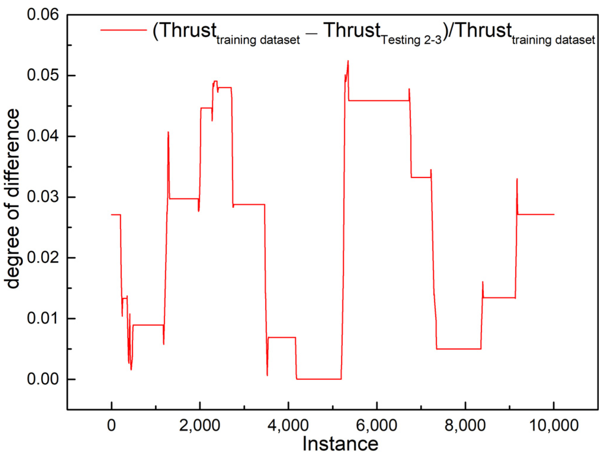
Additionally, it can be observed that the performance of the models on Testing 2-3 is the least favorable when compared to the other testing datasets, suggesting that the disparity between Testing 2-3 and the training dataset is the greatest. Figure 10 shows the thrust value difference between Testing 2-3 and the training dataset. Based on Figure 10 and the outcomes of models Str-5 to Str-7 on Testing 2-3, it can be concluded that a 5% variation between the training and testing datasets is acceptable. Despite a significant reduction in its MRD compared to Testing 1, the LS-1 model performance on Testing 2 remains subpar, with an MRD still above 5%. This could be attributed to the use of distinct component characteristic map in engine performance simulation, resulting in a lower thrust value for Testing 2 than for Testing 1. However, when the predicted thrust value of the LS-1 model is lower than the test data, the model performs better on Testing 2 than on Testing 1.

4. Conclusions

On-board engine health management (EHM) is developed for ensuring aircraft engine reliability. One key component of the on-board EHM is an on-board adaptive model that is responsible for monitoring and predicting engine performance. In this study, we present an on-board adaptive model for predicting engine thrust. The model is built based on a hybrid architecture that combines domain knowledge of the engine with neural network structure. By fusing the aeroengine domain knowledge and neural network structure, the hyperparameters of neural networks are restricted, the interconnections between neural networks are tailored, and the data processing workload is reduced.

To evaluate the effectiveness and robustness of our hybrid architecture, we verified predicting models with different architectures using four simulation datasets. As expected, the hybrid architecture reduces the dependence of the neural network on training data, which is important because engine performance deteriorates over time, leading to differences between the engine state used for model training. In order to be used on an airborne system, the robustness of the on-board model is crucial. Thus, the thrust predicting model built by the hybrid architecture is more suitable for EHM.

References

1. Litt, J.S.; Simon, D.L.; Garg, S.; Guo, T.H.; Mercer, C.; Millar, R.; Behbahani, A.; Bajwa, A.; Jensen, D.T. A Survey of Intelligent Control and Health Management Technologies for Aircraft Propulsion Systems. J. Aerosp. Comput. Inf. Commun. 2004, 1, 543–563. [Google Scholar] [CrossRef]
2. Kobayashi, T.; Simon, D.L. Integration of On-Line and Off-Line Diagnostic Algorithms for Aircraft Engine Health Management. J. Eng. Gas Turbines Power 2007, 129, 986–993. [Google Scholar] [CrossRef]
3. Simon, D.L. An Integrated Architecture for On-board Aircraft Engine Performance Trend Monitoring and Gas Path Fault Diagnostics. In Proceedings of the 57th JANNAF Joint Propulsion Meeting, Colorado Springs, CO, USA, 3–7 May 2010. [Google Scholar]
4. Armstrong, J.B.; Simon, D.L. Implementation of an Integrated On-Board Aircraft Engine Diagnostic Architecture. In Proceedings of the 47th AIAA/ASME/SAE/ASEE Joint Propulsion Conference & Exhibit, San Diego, SA, USA, 31 July–3 August 2011. NASA/TM-2012-217279, AIAA-2011-5859, 2012.. [Google Scholar]
5. Brunell, B.J.; Viassolo, D.E.; Prasanth, R. Model adaptation and nonlinear model predictive control of an aircraft engine. In Proceedings of the ASME Turbo Expo 2004: Power for Land, Sea and Air, Vienna, Austria, 14–17 June 2004; Volume 41677, pp. 673–682. [Google Scholar]
6. Jaw, L.C.; Mattingly, J.D. Aircraft Engine Controls: Design, System Analysis, and Health Monitoring; Schetz, J.A., Ed.; American Institute of Aeronautics and Astronautics: Reston, VA, USA, 2009; pp. 37–61. [Google Scholar]
7. Alag, G.; Gilyard, G. A proposed Kalman filter algorithm for estimation of unmeasured output variables for an F100 turbofan engine. In Proceedings of the 26th Joint Propulsion Conference, Orlando, FL, USA, 16–18 July 1990. [Google Scholar]
8. Csank, J.T.; Connolly, J.W. Enhanced Engine Performance During Emergency Operation Using a Model-Based Engine Control Architecture. In Proceedings of the AIAA/SAE/ASEE Joint Propulsion Conference, Orlando, FL, USA, 27–29 July 2015. [Google Scholar]
9. Simon, D.L.; Litt, J.S. Application of a constant gain extended Kalman filter for in-flight estimation of aircraft engine performance parameters. In Proceedings of the ASME Turbo Expo 2005: Power for Land, Sea, and Air, Reno, NV, USA, 6–9 June 2005. [Google Scholar]
10. Litt, J.S. An optimal orthogonal decomposition method for Kalman filter-based turbofan engine thrust estimation. J. Eng. Gas Turbines Power 2007, 130, 745–756. [Google Scholar]
11. Csank, J.; Ryan, M.; Litt, J.S.; Guo, T. Control Design for a Generic Commercial Aircraft Engine. In Proceedings of the 46th AIAA/SAE/ASEE Joint Propulsion Conference, Nashville, TN, USA, 25–28 July 2010. [Google Scholar]
12. Zhu, Y.Y.; Huang, J.Q.; Pan, M.X.; Zhou, W.X. Direct thrust control for multivariable turbofan engine based on affine linear parameter varying approach. Chin. J. Aeronaut. 2022, 35, 125–136. [Google Scholar] [CrossRef]
13. Simon, D.L.; Borguet, S.; Léonard, O.; Zhang, X. Aircraft engine gas path diagnostic methods: Public benchmarking results. J. Eng. Gas Turbines Power 2013, 136, 041201–041210. [Google Scholar] [CrossRef]
14. Chati, Y.S.; Balakrishnan, H. Aircraft engine performance study using flight data recorder archives. In Proceedings of the 2013 Aviation Technology, Integration, and Operations Conference, Los Angeles, CA, USA, 12–14 August 2013. [Google Scholar]
15. Kobayashi, T.; Simon, D.L. Hybrid neural network genetic-algorithm technique for aircraft engine performance diagnostics. J. Propuls. Power 2005, 21, 751–758. [Google Scholar] [CrossRef]
16. Kim, S.; Kim, K.; Son, C. Transient system simulation for an aircraft engine using a data-driven model. Energy 2020, 196, 117046. [Google Scholar] [CrossRef]
17. Wang, Z.; Zhao, Y. Data-Driven Exhaust Gas Temperature Baseline Predictions for Aeroengine Based on Machine Learning Algorithms. Aerospace 2023, 10, 17. [Google Scholar] [CrossRef]
18. Zhao, Y.P.; Sun, J. Fast Online Approximation for Hard Support Vector Regression and Its Application to Analytical Redundancy for Aeroengines. Chin. J. Aeronaut. 2010, 23, 145–152. [Google Scholar]
19. Zhao, Y.P.; Li, Z.Q.; Hu, Q.K. A size-transferring radial basis function network for aero-engine thrust estimation. Eng. Appl. Artif. Intell. 2020, 87, 103253. [Google Scholar] [CrossRef]
20. Huang, G.B.; Zhu, Q.Y.; Siew, C.K. Extreme learning machine: Theory and applications. Neurocomputing 2006, 70, 489–501. [Google Scholar] [CrossRef]
21. Dong, Y.; Liao, F.; Pang, T.; Su, H.; Zhu, J.; Hu, X.; Li, J. Boosting Adversarial Attacks with Momentum. In Proceedings of the 2018 IEEE/CVF Conference on Computer Vision and Pattern Recognition (CVPR) IEEE, Salt Lake City, UT, USA, 18–23 June 2018. [Google Scholar]
22. Tartakovsky, A.M.; Marrero, C.O.; Perdikaris, P. Physics-Informed Deep Neural Networks for Learning Parameters and Constitutive Relationships in Subsurface Flow Problems. Water Resour. Res. 2020, 56, e2019WR026731. [Google Scholar] [CrossRef]
23. Yang, L.; Zhang, D.; Karniadakis, G.E. Physics-informed generative adversarial networks for stochastic differential equations. SIAM J. Sci. Comput. 2020, 42, 292–317. [Google Scholar] [CrossRef]
24. Karniadakis, G.E.; Kevrekidis, I.G.; Lu, L.; Perdikaris, P.; Wang, S.; Yang, L. Physics-informed machine learning. Nat. Rev. Phys. 2021, 3, 422–440. [Google Scholar] [CrossRef]
25. Van Dyk, D.A.; Meng, X.L. The art of data augmentation. J. Comput. Graph. Stat. 2001, 10, 1–50. [Google Scholar] [CrossRef]
26. Bronstein, M.M.; Bruna, J.; LeCun, Y.; Szlam, A.; Vandergheynst, P. Geometric deep learning: Going beyond Euclidean data. IEEE Signal Process. Mag. 2017, 34, 18–42. [Google Scholar] [CrossRef]
27. Cohen, T.; Weiler, M.; Kicanaoglu, B.; Welling, M. Gauge equivariant convolutional networks and the icosahedral cnn. Proc. Mach. Learn. Res 2019, 97, 1321–1330. [Google Scholar]
28. Raissi, M.; Perdikaris, P.; Karniadakis, G.E. Physics-informed neural network: A deep learning framework for solving forward and inverse problems involving nonlinear partial differential equations. J. Comput. Phys. 2019, 378, 686–707. [Google Scholar] [CrossRef]
29. Robinson, H.; Pawar, S.; Rasheed, A.; San, O. Physics guided neural networks for modelling of non-linear dynamics. Neural Netw. 2022, 154, 333–345. [Google Scholar] [CrossRef]
30. Goodfellow, I.; Bengio, Y.; Courville, A. Deep Learning—Adaptive Computation and Machine Learning Series; The MIT Press: Cambridge, MA, USA, 2016. [Google Scholar]
31. Gers, F.A.; Schmidhuber, J.; Cummins, F. Learning to Forget: Continual prediction with LSTM. Neural Comput. 2000, 12, 2451–2471. [Google Scholar] [CrossRef]
32. Jacobs, R.A. Increased Rates of Convergence Through Learning Rate Adaptation. Neural Netw. 1988, 1, 295–307. [Google Scholar] [CrossRef]
33. Duchi, J.C.; Hazan, E.; Singer, Y. Adaptive Subgradient Methods for Online Learning and Stochastic Optimization. J. Mach. Learn. Res. 2011, 12, 2121–2159. [Google Scholar]
34. Kingma, D.P.; Ba, J. Adam: A Method for Stochastic Optimization. In Proceedings of the 2014 International Conference on Learning Representations, Banff, AB, Canada, 14–16 April 2014. [Google Scholar]
Figure 1. Aircraft engine structure and neural network architecture. (a) A constructure sketch of an aircraft propulsion. (b) A sketch of the architecture enabled by fusing engine structure and neural network.
Aerospace 10 00493 g001
Figure 2. The standard modes of node connection in artificial neural networks.
Aerospace 10 00493 g002
Figure 3. A sketch of an LSTM cell. The arrows in the figure indicate the direction of data transmission.
Aerospace 10 00493 g003
Figure 4. The relationship between the parameters in the predicting model.
Aerospace 10 00493 g004
Figure 5. A sketch of the component-level model of the two-spool mixing exhaust turbofan.
Aerospace 10 00493 g005
Figure 6. The architectures for thrust predicting model. (a) Conventional network architecture. (b) Simple block architecture. (c) Hybrid neural network architecture.
Aerospace 10 00493 g006
Figure 7. The input layers and output layers for each model. (a) AN-1, AN-2, AN-3. (b) Str-5, Str-6, Str-7. (c) LS-1. (d) Str-1, Str-2, Str-3, Str-4. The arrows in the figure indicate the direction of data transmission.
Aerospace 10 00493 g007
Figure 8. The trend of model thrust prediction on testing datasets. (a) Testing 1. (b) Testing 2-1. (c) Testing 2-2. (d) Testing 2-3.
Aerospace 10 00493 g008aAerospace 10 00493 g008b
Figure 9. Histogram on the MRD of the thrust predicting models on testing datasets. (a) Testing 1. (b) Testing 2-1. (c) Testing 2-2. (d) Testing 2-3.
Aerospace 10 00493 g009
Figure 10. The thrust value difference between Testing 2-3 and the training dataset.
Aerospace 10 00493 g010