Article

Deep Reinforcement Learning-Based Failure-Safe Motion Planning for a 4-Wheeled 2-Steering Lunar Rover

1
Korea Institute of Robotics and Technology Convergence, Seoul 06372, Republic of Korea
2
Korea Institute of Robotics and Technology Convergence, Pohang 37666, Republic of Korea
*
Author to whom correspondence should be addressed.
Aerospace 2023, 10(3), 219; https://doi.org/10.3390/aerospace10030219
Submission received: 28 December 2022 / Revised: 18 February 2023 / Accepted: 23 February 2023 / Published: 25 February 2023
(This article belongs to the Section Astronautics & Space Science)

Abstract

:
The growing trend of onboard computational autonomy has increased the need for self-reliant rovers (SRRs) with high efficiency for unmanned rover activities. Mobility is directly associated with a successful execution mission, thus fault response for actuator failures is highly crucial for planetary exploration rovers in such a trend. However, most of the existing mobility health management systems for rovers have focused on fault diagnosis and protection sequences that are determined by human operators through ground-in-the-loop solutions. This paper presents a special four-wheeled two-steering lunar rover with a modified explicit steering mechanism, where each left and right wheel is controlled by only two actuators. Under these constraints, a new motion planning method that combines reinforcement learning with the rover’s kinematic model without the need for dynamics modeling is devised. A failure-safe algorithm is proposed to address the critical loss of mobility in the case of steering motor failure, by expanding the devised motion planning method, which is designed to ensure mobility for mission execution in a four-wheeled rover. The algorithm’s performance and applicability are validated through simulations on high-slip terrain scenarios caused by steering motor failure and compared with a conventional control method in terms of reliability. This simulation validation serves as a preliminary study toward future works on deformable terrain such as rough or soft areas and optimization of the deep neural network’s weight factor for fine-tuning in real experiments. The failure-safe motion planning provides valuable insights as a first-step approach toward developing autonomous recovery strategies for rover mobility.

1. Introduction

In recent years, there has been increasing demand for lunar rovers for Moon exploration missions, with special designs suitable for the extreme environmental conditions of the Moon, and economically feasible hardware. Four-wheeled platforms have received significant attention as promising candidates because they are compact enough to fit the limited space available in launch vehicles while satisfying critical physical requirements [1,2,3].
Lunar rovers are designed as four-wheeled two-steering mobile robots with a shielded body to allow them to tolerate the extreme environmental conditions experienced on Moon exploration missions, including the absence of air and microgravity [4]. They must also meet the physical requirements of the Korean launch vehicles and landing modules in which they are loaded. The rover’s mechanical parts must also ensure the safety of their integrated electrical components, protecting them from the extreme environmental conditions of the Moon. For these reasons, a unique mechanism called modified explicit steering is used for the rover’s steering system. When all of the steering motors work properly, steering control can be achieved by approximating a kinematic model of the target rover, considering its slow-moving speed, and the speed of telecommunication between the Moon and the Earth.
This method, however, has a critical limitation; a failure in even a single steering motor would make it impossible to establish a mathematical dynamics model that is precise enough to be used for robot control due to the resultant recursive effects, which are difficult to mathematically formulate. More specifically, such a failure leads to slipping between the wheel and the ground, which results in the robot body slipping. This then leads to further slipping of the other wheels and the ground.
In addition, existing four-wheeled mobile robots with non-holonomic characteristics exhibit low mobility on the Moon’s surface, where wheel slip is maximized due to microgravity and soft soil [5]. Furthermore, a failure in the steering motor of a rover may affect its wheel alignment. Even when only one of the four wheels becomes misaligned, the overall locomotion of the rover will be significantly affected by slippage [3]. However, most studies on mathematical dynamics models concerning the interaction between the Moon’s surface and the rovers’ wheels have been based on a single wheel–terrain interaction and, thus, the results do not necessarily guarantee that the same degree of controllability would be achieved in four-wheeled systems.
Meanwhile, there has been a sustained interest in the field of fault tolerance and mobility health for planetary exploration rovers. However, many of the studies mainly focus on diagnosis to detect and classify mobility faults or sense errors [6]. Otherwise, most research subjects are close to the implementation of the fault protection sequences through the human decision from a ground-in-the-loop solution [7]. Recently, attention to self-reliant rovers (SRR) is on the rise as well due to the efficiency of unmanned rover activities as onboard computational autonomy becomes advanced [8,9,10,11]. According to a NASA report, multiple hardware failures have been recorded during the first seven years since the landing of the Mars Science Laboratory (MSL) exploration rover on Mars in 2012. The report highlights that one or more failures of steering or driving actuators are classified as primary risks to the rover’s mobility [12]. Another report chooses the increased scope of fault response as one of the remained outstanding challenges in the field. The report emphasizes the importance of autonomous recovery from mobility failures for planetary rovers [13]. In response to these challenges, some works study the development of hardware design toolkits for fault-tolerant systems [14], while others have focused on software architecture based on control allocation to address actuator failures [15]. However, these compensation strategies for actuator failure may not fully address the degree of the rover’s motion planning.
In recent studies, the focus on safety in motion planning of planetary rovers has been explored from various perspectives. Some researchers consider reliable motion planning to be an energy-efficiency issue [16,17,18,19,20,21,22], while others focus on the development of classification and navigation technologies for avoiding hazardous terrain such as deformable or high-slip areas {Egan, #54;Blacker, 2021 #61;Ugur, 2021 #62;Tang, 2022 #65;Endo, 2022 #74;Blacker, 2021 #61}. Additionally, some works concentrate on the rover’s path planning itself, employing classical or learning-based methods [23,24,25]. Simply put, these studies have primarily centered around traversability analysis and the prediction of slippage on rough terrain in the motion planning of rovers.
As part of these efforts, various studies aimed at predicting slippage on rough terrain have been undertaken. Some previous studies focused on estimating the exact degree of slippage [26,27,28,29]. Recent works aim to model wheel–terrain dynamics and calculate traction forces [30,31,32,33]. Additionally, some studies utilize machine learning or reinforcement learning to model the dynamics through the neural networks [34,35,36,37]. However, the common factor among these studies is to develop a more sophisticated wheel–terrain contact model for rough or soft terrain where slippage is likely to occur, with the aim of increasing the controllability of the planetary rover during normal operation without any failure. In addition, it is worth noting that predicting rover slippage accurately is a challenging task, especially on sandy slopes, and the accuracy of the resulting wheel–terrain modeling is uncertain.
The uncertainty associated with actuator failures presents a critical challenge for wheeled rovers, as mobility loss can result in a mission end. Given the inaccessibility of planetary rovers once they are sent into space, it is essential to have a contingency plan in order to address failure scenarios to ensure the successful completion of the mission without loss of mobility. Despite its importance, there is a limited amount of research on developing safe motion planning strategies for potential mobility failures of planetary rovers.
Therefore, we propose a method for failure-safe motion planning that maintains mobility even in events of motor failure. As previously mentioned, machine learning and reinforcement learning methods have been increasingly applied in various technology fields relevant to planetary rovers [38,39]. Thus, in this paper, we present a new reinforcement-learning-based approach for safe motion planning in the presence of actuator failure. This method utilizes only the kinematic model when all motors are functioning correctly, without incorporating any dynamic model such as the wheel–terrain model, even if the robot’s kinematic model cannot be accurately formulated due to unavoidable slip in the event of steering motor failure.
In this paper, a model-free learning approach is proposed for the failure-safe motion planning of a lunar rover. The lunar rover is a four-wheeled, two-steered mobile robot that is subject to loss of mobility in the case of steering motor failure due to the limitation of design and steering mechanism. Reinforcement learning is used to compensate for the unmodeled dynamics effects in the kinematic model in local motion planning by fitting parameters to environments for motor failure. As will be mentioned again later in the paper, the applicability of various model-free learning methods was evaluated and compared with respect to detailed classification criteria (including the state transition probability, the presence of target networks, the capability of calculating high degrees of freedom, and the required time for learning) [40,41,42,43,44,45], while also considering the control inputs of rovers performing as mobile robots with non-holonomic characteristics [46]. As a result, the Deep Q-learning Network (DQN) was selected as the final approach.
The performance of failure-safe motion planning using DQN was verified for Moon exploration missions, which is associated with path planning. The ultimate purpose of a rover is to move from a starting point to a target point. Thus, the primary performance criterion for any rover controller is the success rate of reaching the target point. Because the reference path is linear, the robot can move along the optimal, shortest trajectory if it can approach the reference path as fast as possible, and follow the path until it reaches the target point. Thus, a secondary performance criterion is defined as the ability to approach the optimum path. The next performance criterion is the path-tracking ability, which verifies whether the actual path of the rover generated by the controller matches the given reference path. Two sets of experiments were performed. In the first experiment, the applicability and performance of the failure-safe algorithm were tested not only in a normal state, in which all motors were properly working, but also in a failure state, in which one of the steering motors was out of order. In the second experiment, the reliability of the reinforcement learning-based motion planning method was evaluated, and the results were compared with those obtained from a conventional control method.
The contributions of this paper are:
  • A kinematic model for controlling a four-wheeled Lunar Rover using a modified explicit steering mechanism is presented.
  • A new method for motion planning is proposed by combining the reinforcement learning approach with the robot’s kinematic model without the requirement for dynamics modeling such as a wheel–terrain interaction model.
  • A failure-safe algorithm is proposed as a safe motion planning strategy to address critical mobility limitations in four-wheeled rovers in case of steering motor failure. The algorithm is designed to ensure the execution of the rover’s mission even in the event of motor failure by scaling the above motion planning method.
  • The proposed failure-safe algorithm is validated through simulations on high-slip flat terrain resulting from steering motor failure, serving as a preliminary study prior to testing on rough or soft terrain in future work. Additionally, these works have practical value as the weight values of the deep neural network are pre-optimized through simulation and can be utilized for fine-tuning in subsequent physical experiments.
  • This work represents a meaningful prior study on an autonomous recovery mission execution strategy for SRR with mobility health management and maintenance issues.
This paper is composed as follows. Section 2 provides a description of a four-wheeled two-steering lunar rover equipped with the modified explicit-steering mechanism. Section 3 describes the failure-safe motion planning of the rover using DQN. Section 4 presents experimental results obtained from two different sets of experiments. In the first experiment, the applicability of the failure-safe algorithm was evaluated when there was a failure in the rover’s steering motor, especially with respect to the success rate of reaching the target point, the ability to approach the optimum path, and the path-tracking ability. In the second experiment, the reliability of the proposed motion planning method was compared to that of a conventional control method. Section 5 presents the conclusions of this paper, along with directions for future studies.

2. Hardware Development for a 4-Wheeled 2-Steering Lunar Rover

This section describes the rover that was designed in this paper. It was designed to fulfill the conditions required for moon exploration missions, while meeting the minimum operating requirements, as well as difficult-to-overcome limitations in its steering mechanism, where a failure in one of the two steering motors might result in the complete loss of steering control.

2.1. Development Requirements

Developing lunar rover hardware is generally limited by the physical constraints imposed by the requirements of Moon exploration missions. The maximum weight of a rover is 20 kg because of the limited loading capacity of Korean launch vehicles. The limited space available in lunar landing modules and the extreme environmental conditions of the Moon also critically affect the design of rovers. On Moon exploration missions, objects can be directly exposed to radically changing temperatures, from −153 °C to −170 °C [47], as well as radiation, fine dust, etc., and thus the reliability of the rover’s actuation system should be considered the primary concern in its design.

2.2. Design and Mechanisms

All of the actuators and electronic components of rovers are installed inside a warm box to ensure actuation reliability. Only the mechanical components are exposed to the external environment. The torque generated by actuators inside the box is transmitted to the external wheels via a power transmission mechanism. This actuator-shielded body design not only ensures the overall safety and reliability of the system but also helps reduce its weight and volume.
In lunar rover design, the number of wheels must be as small as possible due to the limited space available in lunar landing modules. Given this constraint, a 4-wheeled system was proposed in this paper. Figure 1 presents the steering mechanisms that are generally used in 4-wheeled systems. Ackermann steering [48,49] and skid steering [50] have been widely used as steering mechanisms for 4-wheeled mobile platforms. While the number of active actuators is small, which is an advantage, these two methods are considered less suitable for the Moon’s environment, where actuation dynamics are more pronounced due to microgravity and the soft soil on the surface. In contrast, general explicit steering requires having the same number of actuators as wheels, and thus explicit steering-based robots tend to be large and heavy, which is not consistent with the ultimate direction of lunar rover hardware development.
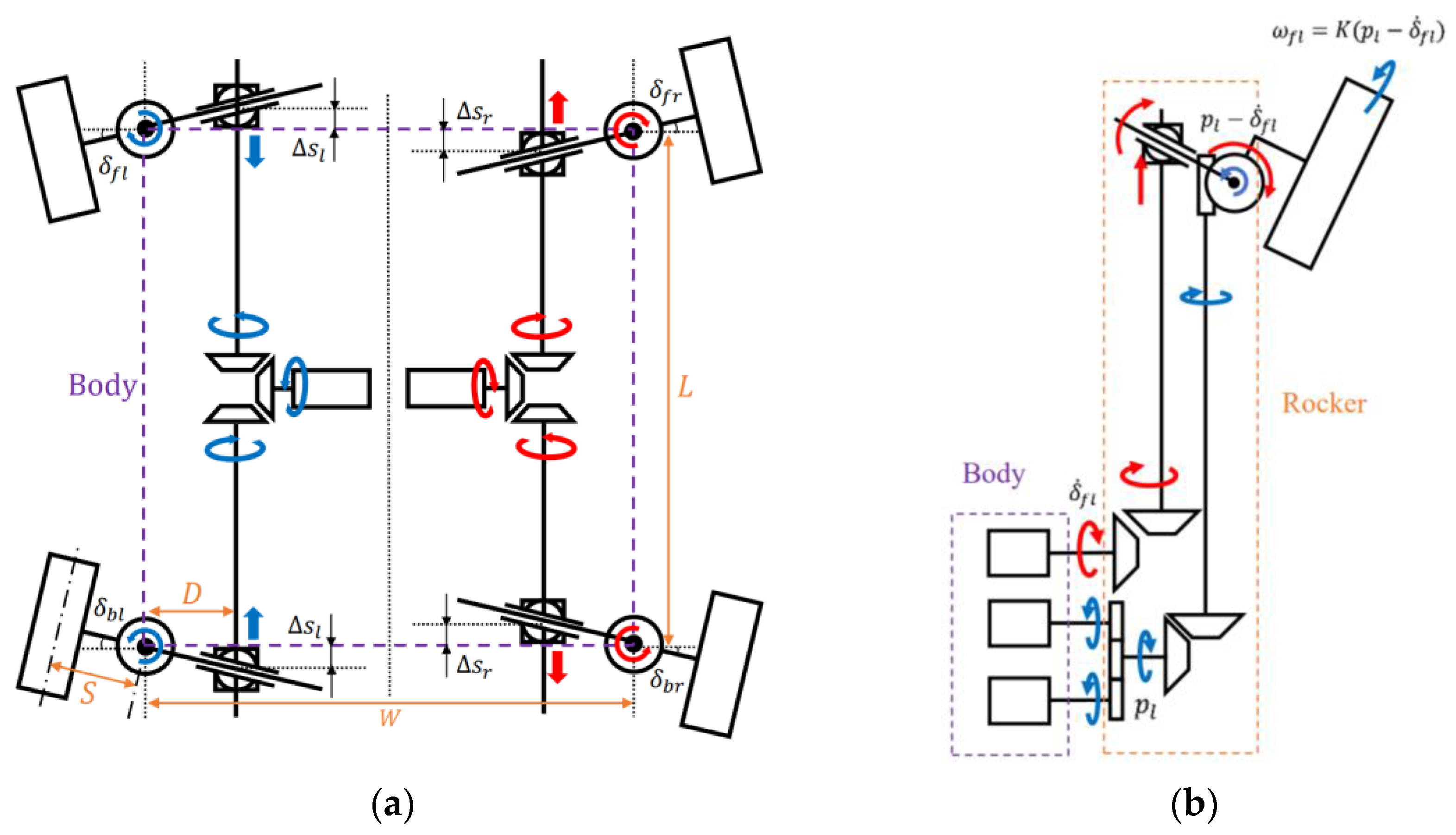
As an alternative, a modified explicit-steering system was devised. This system is relatively less affected by slippage, while still satisfying all the requirements of Moon exploration missions. In this system, a single actuator is coupled to the front and rear wheels on one side through gears and two rockers. As a result, the alignment of the four wheels can be controlled using the internal torque generated by only two steering motors, and these motors are located inside the shielded body of the rover. This configuration is suitable for an actuator-shielded structure.
This modified explicit steering design was finally selected as the steering mechanism for the 4-wheeled lunar rover because it was suitable for the Moon’s extreme environmental conditions while satisfying all physical constraints [4].
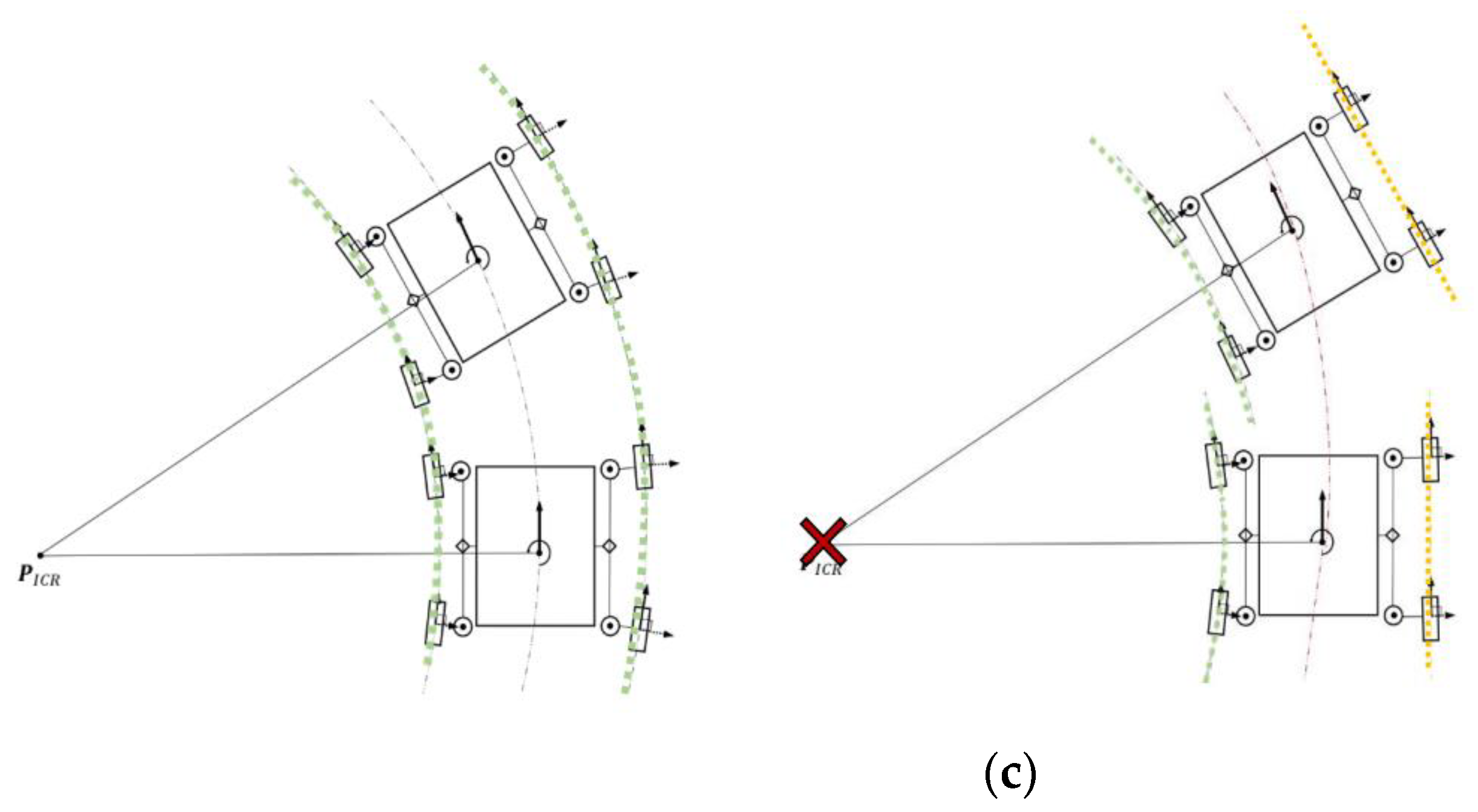
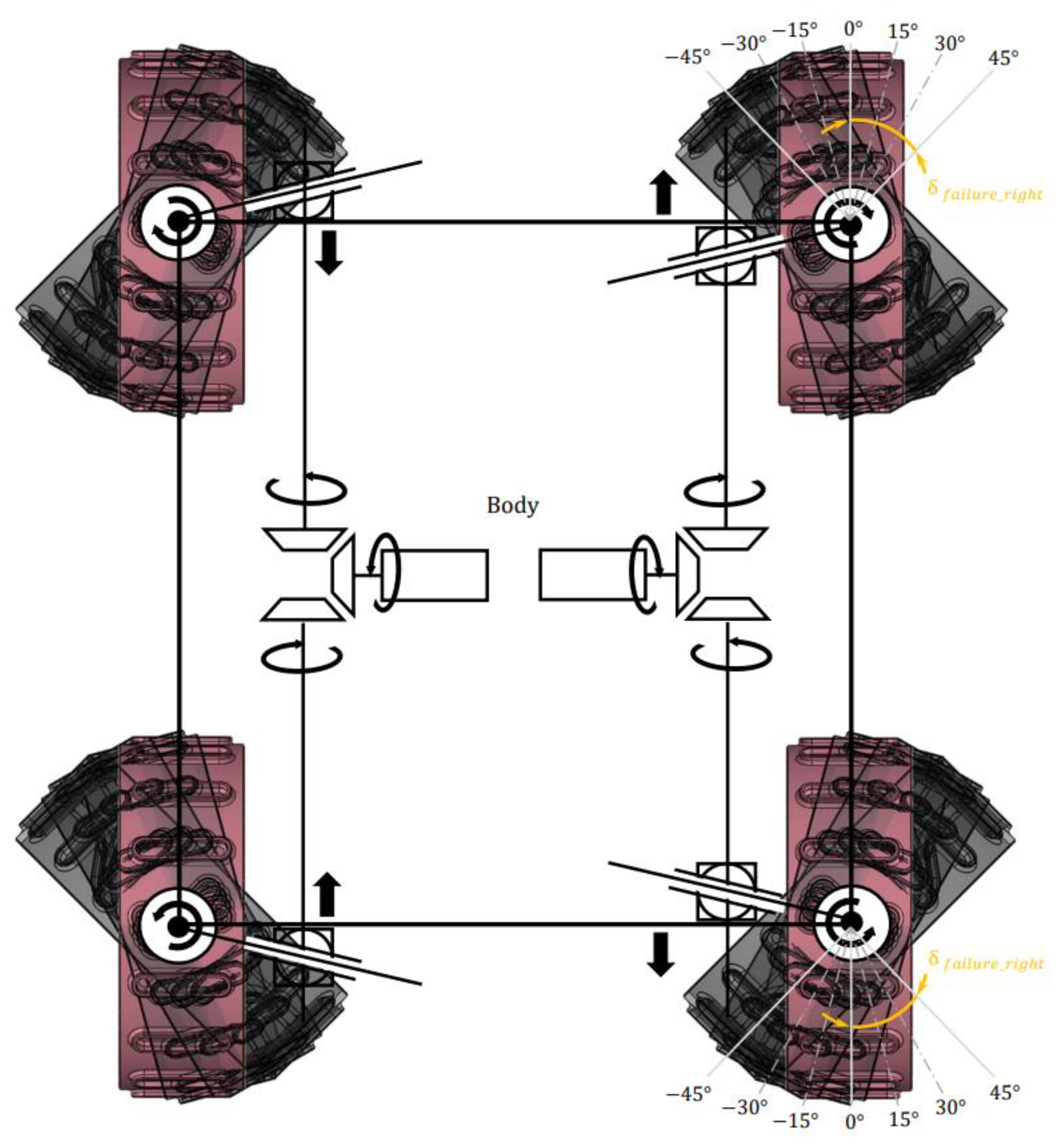
At the same time, a failure-safe design is needed to ensure that the rover can still move, even in case of failure. If the driving motor fails, the rover can end up losing mobility in the forward direction and, thus, will be unable to complete its mission. Therefore, although there is a trade-off relationship between the number of actuators and the weight and volume limits, additional redundancy must be built into the hardware design, especially the driving motors [51]. Accordingly, a dual-motor system was employed in the design of the driving mechanism of the rover [4]. In this system, each coupled set of front and rear wheels on both sides are controlled using two motors, and a total of four actuators were used. As shown in Figure 2a, even if one driving motor of the robot breaks down, the other motor will continue to rotate while also bearing the additional load resulting from the failed motor, i.e., in a hardware backup scenario.
However, despite its various advantages (lighter weight and less affected by wheel slip), the modified explicit-steering system has the disadvantage of increased uncertainty in steering operations even when only one of the steering motors malfunctions.
Figure 2b presents two situations, one in which the right steering motor works properly and one where it breaks down, respectively. Figure 2c illustrates the situation where the steering control of the rover is lost due to the failure of the right steering motor. Due to the addition of actuators in the driving system, there is a physical limit to the degree of hardware redundancy in the steering system. Therefore, a software-level solution must be prepared to respond to a failure in the steering motor, and this will be described in more detail in Section 3.

2.3. Kinematic Modeling

It is very difficult to formulate precise kinematic models for non-holonomic mobile robots with special structural designs, such as lunar rovers [52]. Therefore, the kinematics of lunar rovers need to be approximated, and this requires the following three assumptions [53]. First, from a control perspective, given that explicit steering can minimize slip between the wheels and the terrain, it is assumed that the effect of both lateral and longitudinal slips is insignificant.
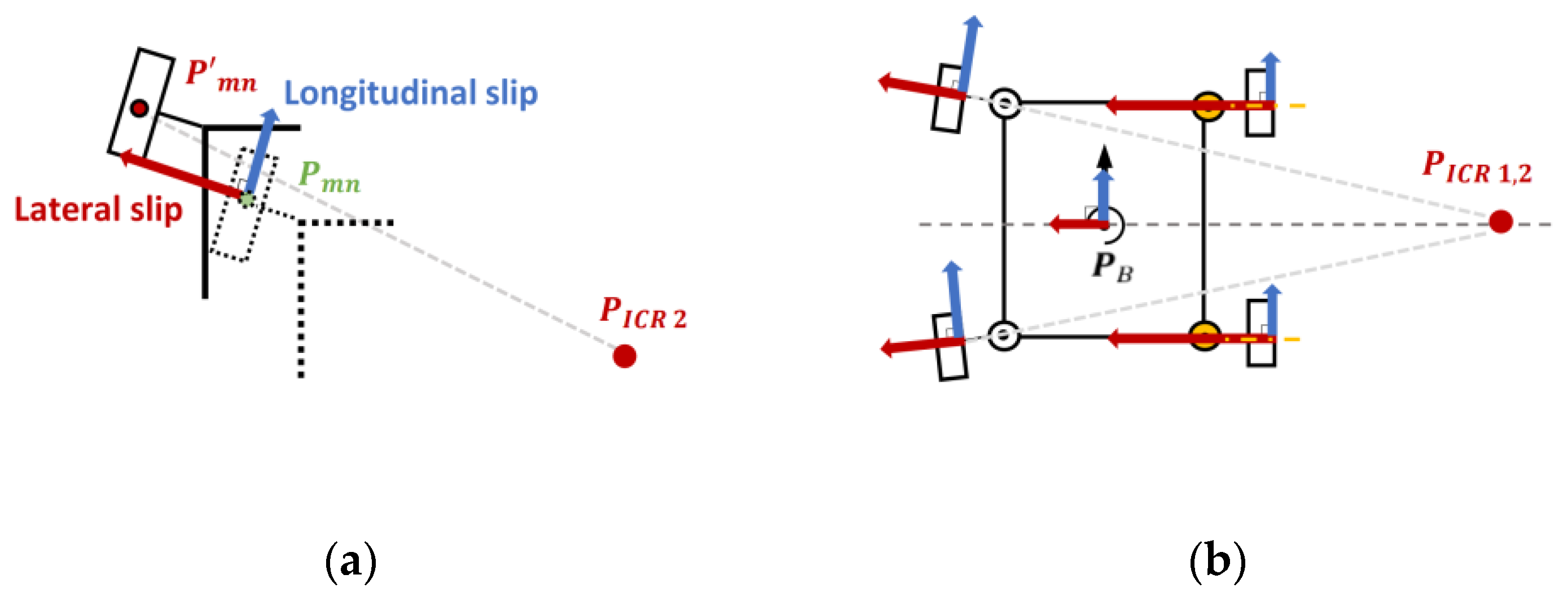
Second, given that the rover moves at a very low speed of about 1 cm/s, lateral slip can be considered insignificant compared to the longitudinal rolling of each wheel. Accordingly, a non-lateral slip condition can be assumed, as shown in Figure 3b. Under this condition, the alignment of each wheel corresponds to the tangential direction of the gyration trajectory of the robot, and thus the rotation center point P m n of each wheel ends up being aligned with the instant center of gyration P I C R .
Therefore, as shown in Figure 4, the distance between this point and the center point of the rover body corresponds to the radius of gyration r of the rover, and thus the alignment of each wheel δ m n can be expressed as in Equations (1) and (2), where L and W refer to the length and width of the robot body, respectively.
tan δ m n = ± L 2 r ± W 2   , δ m n ( π 2   ,   π 2   )
[ δ f l δ f r δ b l δ b r ] = [ arctan L 2 r W arctan L 2 r + W arctan L 2 r W arctan L 2 r + W ]   , δ f l δ b l = δ f r δ b r = 1
As can be seen in Figure 5a, each wheel’s alignment δ m n is controlled by both the lever’s displacement Δ s l and Δ s r and, therefore, the relationship can be expressed as a proportional expression with respect to the revolution of the bevel gear ratio D . Simply put, in the 2D Cartesian frame, the relationship between the steering motor input Δ s l , r and the radius of gyration r of the robot can be expressed as in Equation (3).
Δ s l = D tan δ f l = D tan ( δ b l ) = D L 2 r W Δ s r = D tan δ f r = D tan ( δ b r ) = D L 2 r + W
The last assumption for the approximation of the kinematic model is the pure-rolling condition. This assumption is made based on the fact that the effect of the longitudinal slip of each wheel is also very small due to the slow movement of the rover. If this assumption holds, the relationship v = R ω m n is satisfied, as shown in Figure 3c. Accordingly, in the 2D Cartesian frame, the relationship between the linear velocity v and the dual-motor system’s output rotation speed p n can be determined.
As shown in Figure 4, the radius of gyration l m n of each wheel can be defined as in Equation (4), given its symmetric steering structure, where the constant S refers to the steering offset due to the physical limit of wheel alignment.
l f l = l b l = 1 2 s g n ( 2 r W ) ( 2 r W ) 2 + L 2 S l f r = l b r = 1 2 s g n ( 2 r + W ) ( 2 r + W ) 2 + L 2 + S
By substituting these relationships into Equation (2), the following equation can be obtained:
[ ω f l ω f r ω b l ω b r ] = 1 R ( w [ 1 0 0 1 1 0 0 1 ] [ l f l l f r ] + S [ 1   0   0   1     1   0     0 1 ] [ δ ˙ f l δ ˙ f r ] )
Each wheel’s rolling speed ω m n in Equation (5) can be expressed as a relationship between the radius l m n connecting each wheel and the rotation center point P m n and the angular velocity w of the entire robot trajectory. In addition, ω m n is also associated with the steering velocity of wheel alignment δ ˙ m n , where R refers to the radius of each wheel.
As shown in Figure 5b, ω m n can be expressed as ω m n = K ( p n δ ˙ m n ) , a proportional expression with respect to the composite gear ratio K , and thus Equation (6) can be obtained as follows.
[ ω f l ω f r ω b l ω b r ] = K ( [ 1 0 0 1 1 0 0 1 ] [ p l p r ] + [ 1   0   0   1   1   0     0 1 ] [ δ ˙ f l δ ˙ f r ] )
Finally, given the identical relationship between Equations (5) and (6), a simplified expression, can be obtained as follows.
p l = w K R l f l p r = w K R l f r
Overall, in the 2D Cartesian frame, the angular velocity w of the robot is proportional to the dual motor system’s output rotation speed p n , and accordingly, the linear velocity of the robot can also be controlled by the relationship v = r w .
These results indicate that the kinematic model of the rover can be mathematically approximated in the condition where all motors are working properly [4]. Rover control can be implemented using this approach. More specifically, the forward kinematics can be calculated with respect to motor control inputs Δ s l , r ,   p l , r using the relationships defined in Equations (3) and (7). As a result, the radius of gyration r , and angular velocity w of the rover can be obtained in the 2D Cartesian frame, and the rover’s status x ,   y ,   θ can, accordingly, be controlled, as shown in Figure 3a.
However, a failure in even one of the steering motors leads to a situation in which the locomotion of the rover is inevitably affected by the slip of each wheel, and this means that all the assumptions made above no longer hold, and accordingly, the approximated kinematic model cannot be used. Therefore, for rover control, a new dynamic model that considers the resulting force generated by the slip of each wheel must be developed. As shown in Figure 6 and Figure 7, however, any slip occurring between one wheel of a 4-wheeled mobile robot and the terrain changes the position of the center point of the robot, and this, in turn, affects the slip between each of the other wheels and the terrain.
A wide range of studies have been performed to derive mathematical models that represent the contact dynamics between a single wheel and the terrain, but more complex dynamics between the four wheels as a whole and the terrain have not been sufficiently studied [54]. Going forward, further research is also needed in the area of whole dynamics modeling, which focuses on the slip between the body of 4-wheeled mobile robots and the terrain [55].
It is also very difficult to formulate contact dynamics with respect to the slip between each wheel and the terrain in an environment where the terrain conditions are constantly changing over time. Furthermore, even if such modeling was possible, the calculation drawn from the process would not be suitable for the real-time control of robots in unconstructed terrains, as on the Moon’s surface.

3. Failure-Safe Motion Planning

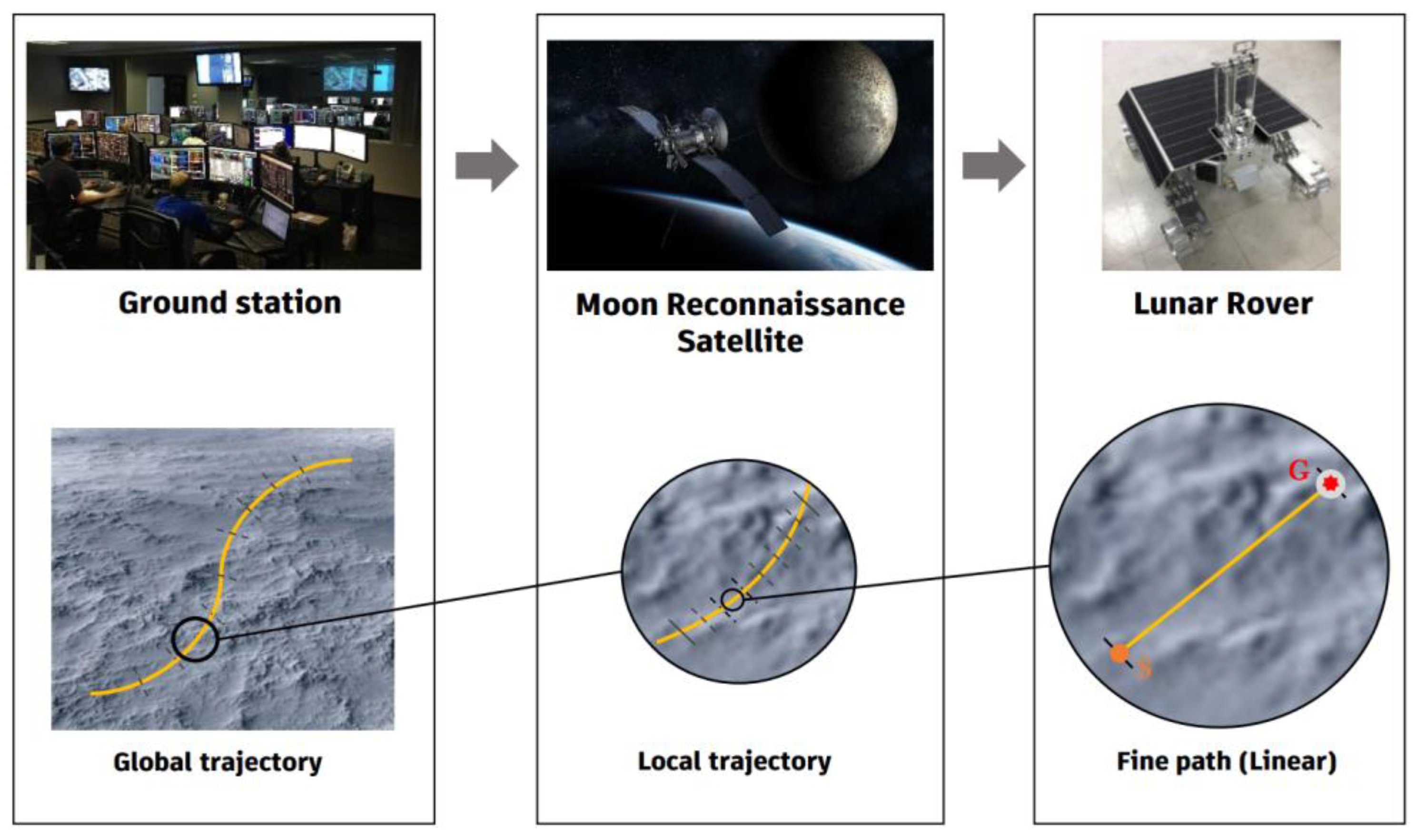
For a Moon exploration mission, the global trajectory of the rover generated by the ground station is segmented into sets of local trajectories before being delivered, due to time delays and the rover’s slow-moving speed. Each local trajectory is further subdivided into sets of fine paths at the sequence level before being transmitted to the rover.
Accordingly, in this process, the actual path that the rover is supposed to follow within each command cycle becomes optimized as a linear path that connects the starting point and the target point. Figure 8 presents the whole procedure for segmenting the global trajectory of the rover generated by the ground station, transmitting the segmented trajectory data to the lunar reconnaissance orbiter, and finally transmitting a fine path data at the sequence level to the rover.
From the rover’s point of view, if it is able to closely follow the given linear path for each sequence in a repeated manner, it will ultimately reach the target point not only through the local trajectory, but also the global trajectory. Simply put, on a Moon exploration mission, the rover is required to follow given sets of linear paths while minimizing the spatial error between the given trajectory and the center point of its main body.

3.1. Reinforcement Learning-Based Motion Planning

As earlier discussed in Section 2, no kinematic or dynamic models are available to simulate lunar rover control of a rover that experiences a failure in its steering motor. Thus, a model-free control approach is required to address this issue. Reinforcement learning (RL) has been proposed as a solution to rover motion control in such a situation, because it avoids the limitations of conventional control methods, which require well-formulated models. As shown in Figure 9, model-free learning can be used for the whole dynamics of the system, and is effective to not only address locked-wheel issues caused by motor malfunctions, but also to maintain controllability, even in free-wheeling conditions resulting from encoder malfunction.
As shown in Figure 10, RL can be largely divided into model-based learning and model-free learning according to the probability of state transition [41]. In lunar rover control, state transition probabilities, which correspond to kinematic or dynamic models, cannot be mathematically formulated in the event of a failure in the steering motor [45]. Alternatively, model-free learning is employed as a solution for failure-free motion planning. Off-policy learning is a type of model-free learning where updating a current policy requires a target policy [56,57]. In rover motion planning, the target policy is defined as a policy that minimizes the distance from the optimal path.
Meanwhile, among off-policy learning methods, the policy-search approach is more advantageous than the value-search approach, in that fewer calculations are required to solve high-DOF problems [43]. Robot control algorithms are implemented in high dimensions because many variables are involved, and thus the policy-search approach is considered more suitable for rover motion planning applications [58]. Q-learning, one of the most widely used policy-search algorithms, is suitable for use in robot control, but requires a long learning time [40,42]. Therefore, Deep Q-Learning Network (DQN), with excellent scalability for high DOF motions and reduced learning time, is proposed as the final solution to failure-safe motion planning for the lunar rover [44,59].

3.2. Failure-Safe Algorithm Using Deep Q-Learning Network (DQN)

3.2.1. Architecture of DQN

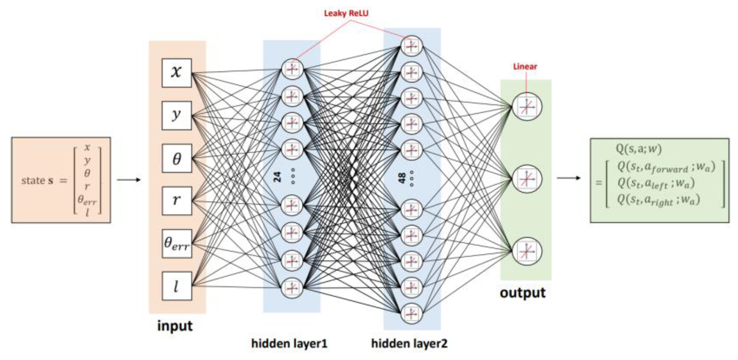
The overall structure of the DQN is presented in Figure 11. This neural network receives six inputs related to the current state of the robot and produces three types of actions as outputs. The network contains two hidden layers that use Leaky-ReLU as an activation function, as well as a mean squared error (MSE)-type loss function. Its optimizer is composed of Adam [60].
First, six inputs concerning the observed current state of the rover, i.e., x , y , θ , r , θ e r r , and l , are entered into the input layer. Subsequently, each observation state value is allowed to pass through two hidden layers that have a non-linear activation function. The first hidden layer is composed of 24 nodes, while the second one is composed of 48 nodes. The yaw θ and yaw error θ e r r , among the observation values, may have negative values, and, therefore, the two hidden layers are designed to have Leaky-ReLu as an activation function. In general, the ReLu function is favored as an activation function because of its high speed, but in this DQN model, both the yaw of the rover body and the yaw error in the target point direction serve as the criteria for reward distribution and, thus, ignoring these factors may lead to biased learning. Accordingly, the Leaky-ReLu function was employed to influence a given policy even with negative values while still providing the same advantages as the ReLu function [61].
Since this model aims to solve regression problems rather than perform classification, a linear function is used as the final output layer. The output function of the final layer is the action-value function Q ( s , a ; w a ) , in which an output is obtained by allowing a given agent to take each action a in the state s [62]. The difference between Q and the optimal Q * is expressed as L ( w a ) , a mean squared error-type loss function. At each iteration, the weight w a is updated to minimize the loss function. Simply put, in this process, the model learns to take actions to allow Q to become closer to the target Q * in Equation (8) [59].
Q ( s , a ; w a ) = x ( s ) T w a
Q * ( s ,   a ; w a ) = E [ r e w a r d + γ max a Q ( s , a ) ]
L ( w a ) = 1 2 [ Q * ( s ,   a ; w a ) Q ( s , a ; w a ) ] 2

3.2.2. State

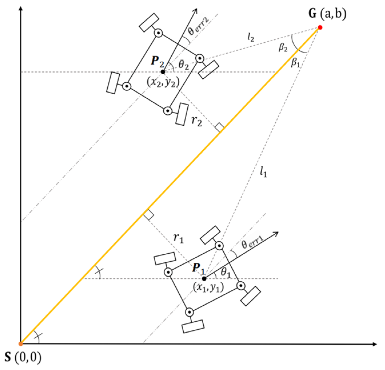
A lunar reconnaissance orbiter orbits around the Moon while observing the rover from a direction perpendicular to it at all times. Thus, the position of the rover can be expressed on a 2D Cartesian coordinate system, as shown in Figure 12. The current position of the rover ( x and y ) and the target point of a given linear path ( a and b ) are observed in the environment. In addition, the remaining distance between the current position of the rover and the target point ( l t ), the azimuth error between the target point direction and the rover moving direction ( θ e r r t ), and the vertical distance between the current position of the rover and the linear path ( r t ) can be accordingly calculated. As a result, a total of five variables are selected as a state group. Equations (11) and (12) present the definition of the state group s t and equations used to calculate the variables l t , θ e r r t , and r t are included in the state group.
{ s s t a r t ,   , s t 1 , s t , s t + 1 , , s g o a l } S s t = ( x t ,   y t ,   θ t ,   r t ,   θ e r r t , l t )
l t = | P t G | = a x t ,   b y t 2 θ e r r t = tan 1 b a + β t θ t = tan 1 b a + cos 1 x t , y t · a , b x t , y t × a , b θ t r t = | P t G | cos β t = l t sin β t = l t sin ( cos 1 x t , y t · a , b x t , y t × a , b )

3.2.3. Action

The dual-motor system’s output rotation speeds p l , r have continuous values. Because the rover is controlled by a signal sampled during the data processing process, these values need to be discretized. When continuous action values are available to select, a very long learning time and high computing power are required.
Accordingly, in this paper, the action group was set to have only three different options by fixing the control inputs of the forward kinematics used in the situation where the steering system worked properly. The approximated kinematic model cannot be used in the case of a failure, but in a normal state, motion planning is performed through learning. The robot can be controlled as desired using only three different steering motions, which are implemented when each set of specific inputs is entered. Simply put, the linear velocity v , angular velocity w , and gyration radius r g were fixed at specific values, and accordingly, the action group was set to have only three moving directions a f o r w a r d , a l e f t , and a r i g h t , as shown in Equation (13).
{ a f o r w a r d , a l e f t , a r i g h t } A a f o r w a r d   :   p l , r = 1 K R v     a l e f t ,     r i g h t   :   p l = ± r g l K R w ,     p r = ± r g r K R w

3.2.4. Reward

The reward can be determined by the amount of variation per unit action in the variables r t , θ e r r t , and l t described above. Basically, in a reward strategy, the smaller the three criteria values are, the larger the reward the agent receives. Rewards are provided differently based on the threshold for each criterion. Reward discrimination thresholds should be set to appropriate constants, considering the sophistication of the desired motion control. Rover motion planning aims to allow the robot to approach the optimal reference path as quickly as possible and follow the path, thereby allowing it to reach as close as possible to the target point. Three reward discrimination thresholds are set to train the robot to perform such desired motions.
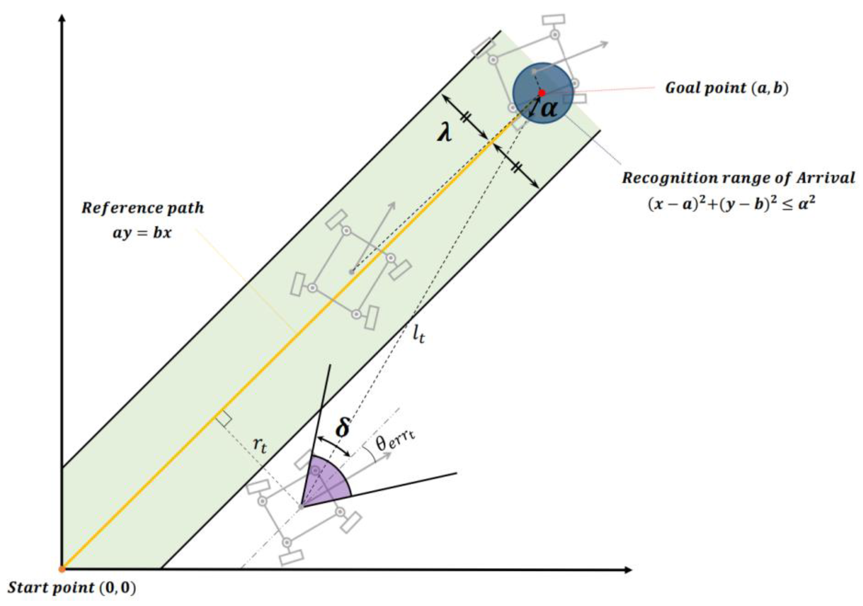
Threshold values, including the distance λ , angle δ , and area α , refer to margin ranges for r t , θ e r r t , and l t , respectively. Learning intensity can be controlled by adjusting these constants. More specifically, the smaller the set margin value is, the more rigorous the reward strategy becomes; this means that the robot can be trained to perform more detailed motions. Accordingly, the λ value should be set smaller to allow the robot to approach the reference path faster and stay closer to the path while driving. If one intends to reduce the possibility that the robot will deviate from the reference path and improve its ability to stay close to the path, the δ value must be reduced.
In addition, a smaller α value is necessary to increase the success rate of reaching the target point with improved spatial accuracy. However, the size of these threshold values is in a trade-off relationship with the required learning time. Smaller threshold values are advantageous for implementing more sophisticated motions, but at the same time, require longer training time. Therefore, appropriate threshold values must be set considering all relevant factors together.
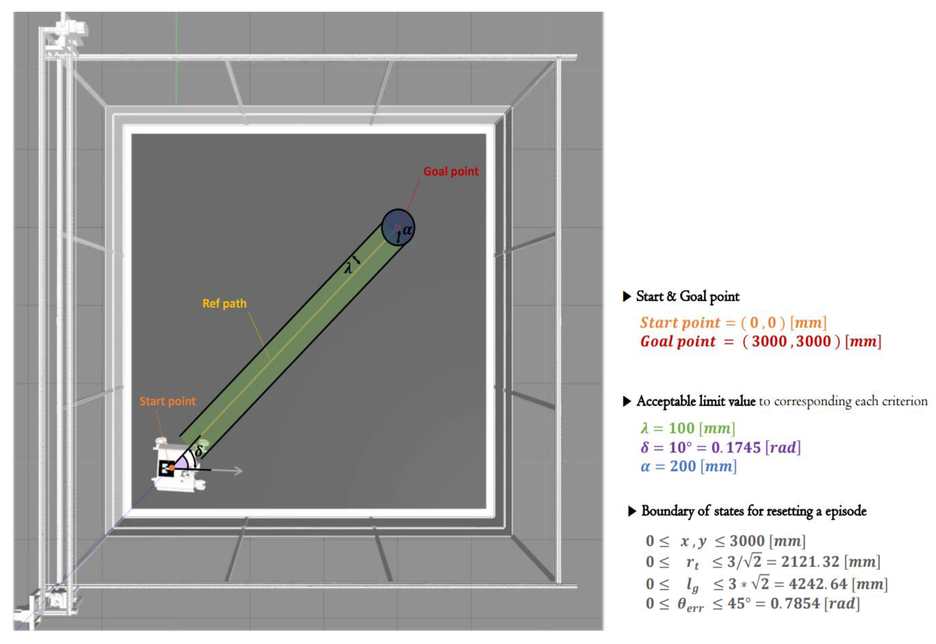
It is also necessary to ensure that each criterion has the same scale so that they have the same degree of effect on the reward during the learning process. Normalization is also performed to maximize the effect of learning with respect to changes in the criteria values. As a result, each normalized reward r e w a r d N ends up between 10 and 100 in an exponential function. These criteria and thresholds can be expressed on a 2D Cartesian Coordinate system, as shown in Figure 13.
The overall reward strategy is presented in Algorithm 1. In motion planning for lunar rovers, the primary motion required for rovers is to approach the reference path as fast as possible. Three reward discrimination thresholds are used in strategy development to train the robot to perform the motion. First, the distance threshold λ determines the margin range. If the distance between the reference path and the robot is within the margin range, the robot is considered to have approached the reference path. Reward strategies are usually divided into two, according to the distance threshold λ .
Algorithm 1 Reward strategy algorithm
1 :   Select   reward   discrimination   thresholds   ( λ ,   δ ,   α )
2 :   Set   the   constant   reward   that   is   given   when   a   sin gle   episode   is   done   to   r e w a r d D = P
3 :   Initialize   the   reward   per   unit   step   r e w a r d S = 0
4 :   Get   old   state   values   ( r t 1 ,   θ e r r 1 , l t 1 )
5 :   Get   new   state   values     ( r t ,   θ e r r , l t )
6 :   Calculate   the   gradient   of   observation   values   ( r t ,   θ e r r , l t )
7 :   Normalize   new   state   values   ( r t ^ ,   θ ^ e r r , l t ^ )
8 :   Calculate   the   normalized   reward ,   r e w a r d N = [ ( 1 100 ) 1 2 r t ^ 1 , ( 1 100 ) 1 2   θ ^ e r r t 1 , ( 1 100 ) 1 2 l t ^ 1 ] T
9 :   Calculate   the   episode   success   coefficient   S c = ( 1 10 ) θ ^ e r r t
10 :   Calculate   the   episode   failure   coefficient   F c = 10 l t ^ 1
11 :   if   the   episode   is   done   and   ( 0 l t α )   then
12 :       r e w a r d T = r e w a r d T + r e w a r d D · S c   ( SUCCESS )
13:   else
14:          if the episode is not done then
15 :                   r e w a r d T = r e w a r d T + r e w a r d S from the Reward discrimination table in Figure 14.
16 :           else   r e w a r d T = r e w a r d T r e w a r d D · F c   ( FAILURE )
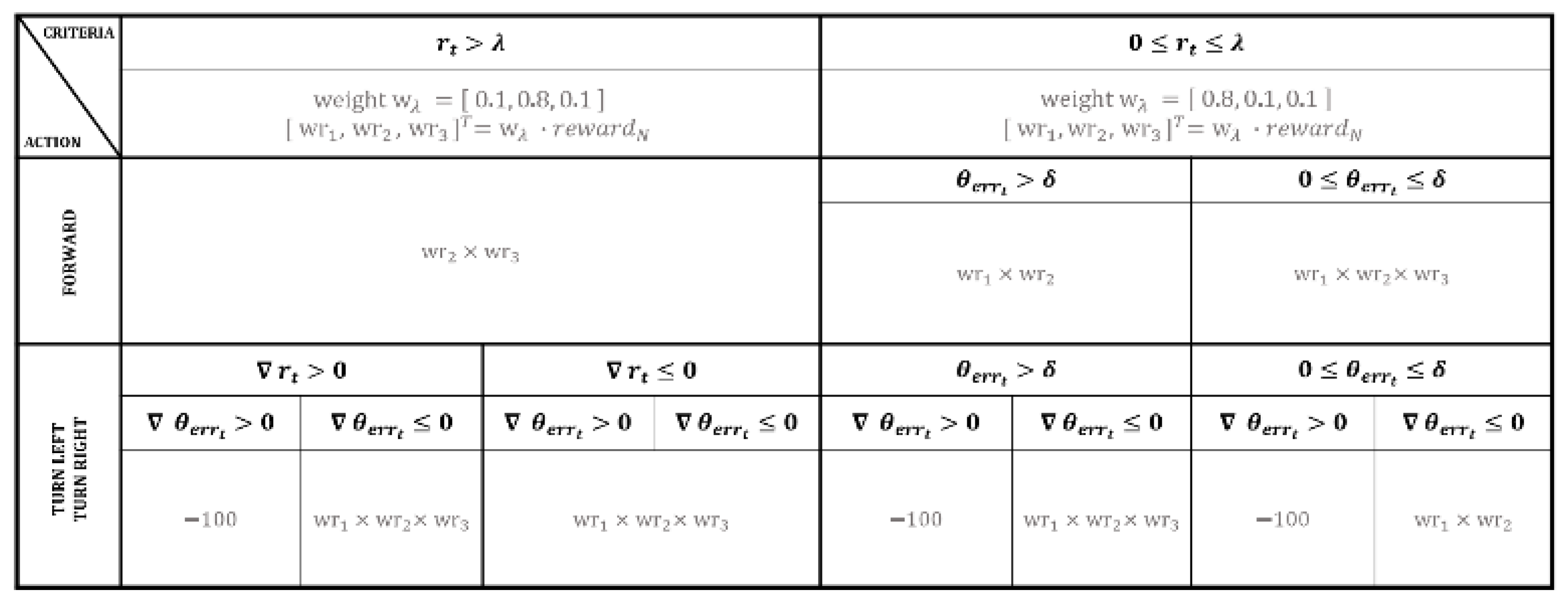
If r t > λ holds, the reward granted by r t , among the three observation variables used to induce the robot to perform the motion, is given the highest weight factor ( wr 2 = 0.8 ). In this case, turning actions are more effective than forward-moving actions to help the robot approach the reference path as fast as possible. Therefore, the highest reward is provided when the robot makes a turn to come closer to the reference path. These conditions are presented in the left column of Figure 14. When r t 0 and r t > 0 & 0 θ e r r t hold, the highest weight factor wr 1 × wr 2 × wr 3 is given. However, if the robot makes a turn to become more distant from the reference path ( r t > 0 & θ e r r t 0 ), a negative reward of 100 is given, which is large enough for the weight factor to be ignored.
In contrast, if 0 r t λ holds, where the robot is considered to have approached the reference path, different weight factors are given to the three observation variables. Once the robot approaches the reference path, the next motion required for the robot is to continue to faithfully follow the path. Accordingly, the highest weight factor ( wr 1 = 0.8 ) is given to the orientation error θ e r r to increase its effect on the overall reward. As can be seen in the right column of Figure 14, the angle threshold δ serves as a critical factor that determines the overall weight factor. In this process, the robot is induced to follow the reference path while maintaining the yaw value toward the target point. If 0 θ e r r t δ holds, the yaw of the robot is considered to be aligned with the direction of the target point within the allowable error limit. Therefore, the current orientation of the robot must remain the same.
Forward-moving actions are given the highest weight factor ( wr 1 × wr 2 × wr 3 ) because they lead to the smallest change in the orientation of the robot. In contrast, if θ e r r t > δ holds, the yaw of the robot is significantly misaligned with the direction of the target point. Therefore, it is necessary to adjust the orientation of the robot, thereby reducing the orientation error. Since turning actions result in a larger change in the robot’s orientation than forward-moving actions, the highest reward is given when θ e r r t 0 holds. However, turning actions in a direction that increases the orientation error (e.g., θ e r r t > 0 ) instead lead to an increase in the azimuth error from the direction of the target point. Therefore, in this case, a negative reward is given. Overall, once the robot is deemed to have approached the reference path closely enough, the top-priory motion required for the robot is to reduce the orientation error from the direction of the target point.
The final reward discrimination threshold is the success radius α . If the robot is within the radius α of the target point, the corresponding episode is considered to be a success. As mentioned in Lines 11 and 12 of Algorithm 1, the remaining distance between the final position of the robot and the target point in a given episode is calculated, and if the calculated value is within the range of 0 l t α , an episode success reward is additionally given. However, if l t > α holds at the end of the episode, the episode failure reward with a negative value is given, thereby deducting the final cumulative reward.
In summary, this reward strategy trains the robot to perform actions in a way that maximizes the final cumulative reward; therefore, once the robot is deemed to have approached the reference path closely enough, it continues to move toward the target point while staying as close to the path as possible and finally reaches as close as possible to the target point. In the proposed method, the robot can be trained to perform desired motions by appropriately adjusting the reward strategy based on changes in the state variables. Therefore, this method is suitable for use in rover motion planning, even when a steering motor fails, and when changes in the position of the rover caused by each action are difficult to expect.

3.2.5. Learning Procedure for the Failure-Safe Algorithm

The learning procedure for the rover’s failure-safe algorithm is represented in Algorithm 2. This algorithm is divided into a training episode, in which the neural network is optimized, and a test episode, where the performance of the trained neural network is verified. Once the rover as an agent completes a random action in a single training episode, the corresponding step is finished. Subsequently, changes in the state variables are observed from the environment, and then used to calculate the r e w a r d N value. This value is then used together with the specific thresholds λ , δ , and α set to improve motion planning performance and provide the reward per unit step r e w a r d S in accordance with the reward discrimination table.
As these steps are repeated in a single episode, rewards tend to cumulate. Once the rover reaches the target point, or the deviation criterion is exceeded by a specific amount, the corresponding episode comes to an end. If the episode is finished before the rover reaches the target point, the corresponding episode is considered to be a failure, deducting the reward by the amount of r e w a r d D · F c . In contrast, if the rover reaches within a certain radius of the target point, the corresponding episode is considered to be a success, and the additional reward r e w a r d D · S c is provided. Once every single episode is finished, the final cumulative reward r e w a r d T is calculated based on the results. By doing so, the loss function L ( w a ) is calculated, and the weight factor w a of the neural network is accordingly updated via backpropagation in a way that minimizes the loss. A group of random actions to be performed in the next learning episode is determined from this updated neural network.
Once the next episode begins, the multiple-step sequence proceeds in the same way as previous episodes. Similarly, once the episode is completed, the final cumulative reward r e w a r d T is calculated, and w a that fulfills a r g m i n w a L ( w a ) is determined to train the neural network. Subsequently, as the number of learning episodes increases, w a is optimized to determine a group of actions that can maximize the cumulative reward.
To select an action per step during learning progress, the ε –greedy policy is employed [63]. Line 11 of Algorithm 2 shows how to determine the robot’s action value in accordance with the random variable p. if p < ε does not hold, the optimal action is selected to maximize the value of the action-value function Q among the three options. In contrast, one of the action groups is randomly selected for the diversity of learning sample data when p < ε holds. In this paper, parameters associated with ε—greedy policy was determined from repeated experiments to guarantee the performance of the policy and that learning time is not too long. The probability values were set as follows: ε m i n = 0.10 , ε = 0.99 , and ε d = 0.99 . The probability of selection ε is updated until ε ε m i n holds at each iteration per action as shown in Line 25 of Algorithm 2.
Algorithm 2 Failure-safe algorithm using Deep Q-learning Network
1 :   Initialize   the   replay   memory   D to the capacity N
2 :   Initialize   the   action - value   function   Q   with   random   weight   factor   w a
3 :   Initialize   the   target   of   action - value   function   Q *   with   the   above   weight   factor   w a
4 :   Initialize   the   batch   size   B ,   the   minimum   of   probability   ε m i n ,       the   probability   of   selection   ε ,   and   the   decaying   factor   of   probability   ε d
5 :     for   e = 0 ,   t h e   n u m b e r   o f   t r a i n i n g   e p i s o d e s   do
6 :     Initialize   the   final   cumulative   reward ,   r e w a r d T = 0
7 :     Initialize   the   initial   state   value   s 0 = ( x 0 ,   y 0 ,   θ 0 ,   r 0 ,   θ e r r 0 , l 0 )
8 :     Initialize   the   preprocessed   state   ϕ 0 = ϕ ( s 0 )
9 :     Initialize   the   flag   of   the   episode s   termination ,   d o n e = F a l s e
10 :         while   d o n e T r u e   do
11 :         Select   an   action   a t = {   r a n d o m ( a f o r w a r d , a l e f t , a r i g h t )     if   random   p < ε a r g m a x w a Q ( ϕ ( s t ) , a t ; w a )             otherwise          
12 :         Get   new   state   values   s t = ( x t ,   y t ,   θ t ,   r t ,   θ e r r t , l t )
13:      Change the flag of the episode’s termination,
        d o n e = {   F a l s e     if   all   observation   values   are   under   the   boundary   condition   T r u e     otherwise                                                                                            
14 :         The   reward   is   given   in   accordance   with   Algorithm   1 .
15                 Get   the   final   cumulative   reward   and   save   it ,   r e w a r d = r e w a r d T
16 :             Put   the   next   state   s t + 1 = ϕ ( s t )
17 :             Start   the   Experience   replay :
18 :                     Store   the   state   value   s t in the replay memory D
19 :                     Select   the   size   of   mini   batch ,   m i n i b a t c h = min ( D ,   B )
20 :                     for   t = 0 ,   m i n i b a t c h   do
21 :                         Q = Q ( ϕ ( s t ) , a t ; w a )
22 :                         Q * = {   r e w a r d                                           if   d o n e = T r u e   r e w a r d + γ max a t + 1 Q ( s t + 1 , a t + 1 )     otherwise          
23 :                     Compute   the   loss   function   L ( w a ) = 1 2 [ Q * Q ] 2
24 :                     Update   the   weight   factor   w a   in   which   a r g m i n w a L ( w a )   is   satisfied
25 :                     if   ε > ε m i n   then   ε = ε · ε d
Meanwhile, as presented in Line 17 of Algorithm 2, the Experience replay method is used to ensure data usage efficiency and address the high correlation issue between state values during the learning process. The replay memory D and batch size B were set to 100 , 000 and 512 , respectively, considering the size of the state group and the learning time as well. During the memory replay process in which t < m i n i b a t c h holds, action-value function Q and target function Q * are calculated. In Line 22 of Algorithm 2, reward decaying factor γ is associated with how fast the agent learns biased policy and how fewer trials for the exploration are; this means that the closer this factor value to 1 is selected, the future reward is regarded as more significant than the current reward. Simply put, a reward is effectively provided when the robot takes action for exploration rather than exploitation. Therefore, this factor was set to γ = 0.95 , in which the trade-off relationship between learning time and learning performance was considered in the rover’s motion planning problem. After all replay, the optimal next action value is determined by computing the loss function L(wa) as shown in Line 23 of Algorithm 2. The last line of Algorithm 2 shows that the weight factor of Deep Neural Net, w a , in which the loss function is minimized, is updated.
The w a values of the neural network optimized for each steering motor failure case are stored as parameters in the onboard controller of the rover.
As shown in Figure 15, the steering angle range of a single wheel is limited to 45 ° to 45 ° due to design constraints. Failure angle analysis is discretized into specific ranges, as a failure-safe solution cannot be achievable for all continuous angles in the event of failure. In this paper, the failure cases of a single steering motor are categorized into seven discrete failure angles. Subdividing this failure angle further would increase the required learning time, but it could enhance control performance and failure safety in motion planning. The failure angle is estimated using the positional errors of the encoders when the motor is locked in a position due to malfunction. If the angle falls between categorized discrete angles, the nearest discrete boundary angle within the range is selected as the failure angle. There are 49 possible cases for steering motor failure in a 4-wheeled, 2-steering lunar rover, considering both left and right steering motor failures. Thus, prior experiments are performed to obtain the w a values for each case, which are then stored as parameters. These parameters would be later utilized in the motion planning of the rover in the event of each actual failure case.
In summary, this method is used for rover motion planning not only in a normal state but also in the case of a failure in the steering motor, when controllability cannot be guaranteed. This failure-safe algorithm is of greater significance for that reason. Once the number of training episodes exceeds a certain level, the neural network with optimized weight factors is used to repeat test episodes. Based on the results, the motion planning performance of the DQN as a failure-safe solution is verified.

4. Experiments

4.1. System Setup

The deep neural network model DQN was implemented using Keras [64], a deep learning library. The failure-safe algorithm was developed using OpenAI Gym [65], an algorithm development library for reinforcement learning. The entire learning process for motion planning was performed based on an interaction with a test environment established via ROS Gazebo simulations [66].
A 3D model of the full-scale lunar rover built in this paper was employed, and the model was designed to have the same mechanical properties as the actual rover, especially with respect to the mass, inertia, gear ratio, etc., as shown in Figure 16, to closely simulate the experimental results obtained in the Gazebo simulation environment. In addition, the static and kinetic friction coefficients of the actual testbed floor on which rover moving experiments were performed were measured and applied to the simulation environmental variables, to faithfully replicate the real-life slip between the rover’s wheels and the ground, ensuring that the approximated physical interactions were implemented in the simulation environment as well in order to obtain closer results for applying to the actual rover. The wheel–terrain interaction model is simplified to the point contact model because the single tip of the wheel’s grouser contacts the surface sequentially while the wheel is rolling due to the slow movement of the rover. Uncertainty about this wheel–terrain interaction model is compensated by the reinforcement learning method while interacting the robot’s wheel model with the testbed environment through the dynamic engine of simulation.
Future works will be conducted on physical robots and test beds to achieve the sim-to-real goal. The nature of reinforcement learning algorithms requires preceded numerous trial-and-errors. However, it is challenging to consistently repeat them under the same conditions in physical experiments. To address this issue, we first optimize the weight value of the deep neural network through simulation. The pre-optimized weight value is then utilized for fine-tuning in physical experiments.
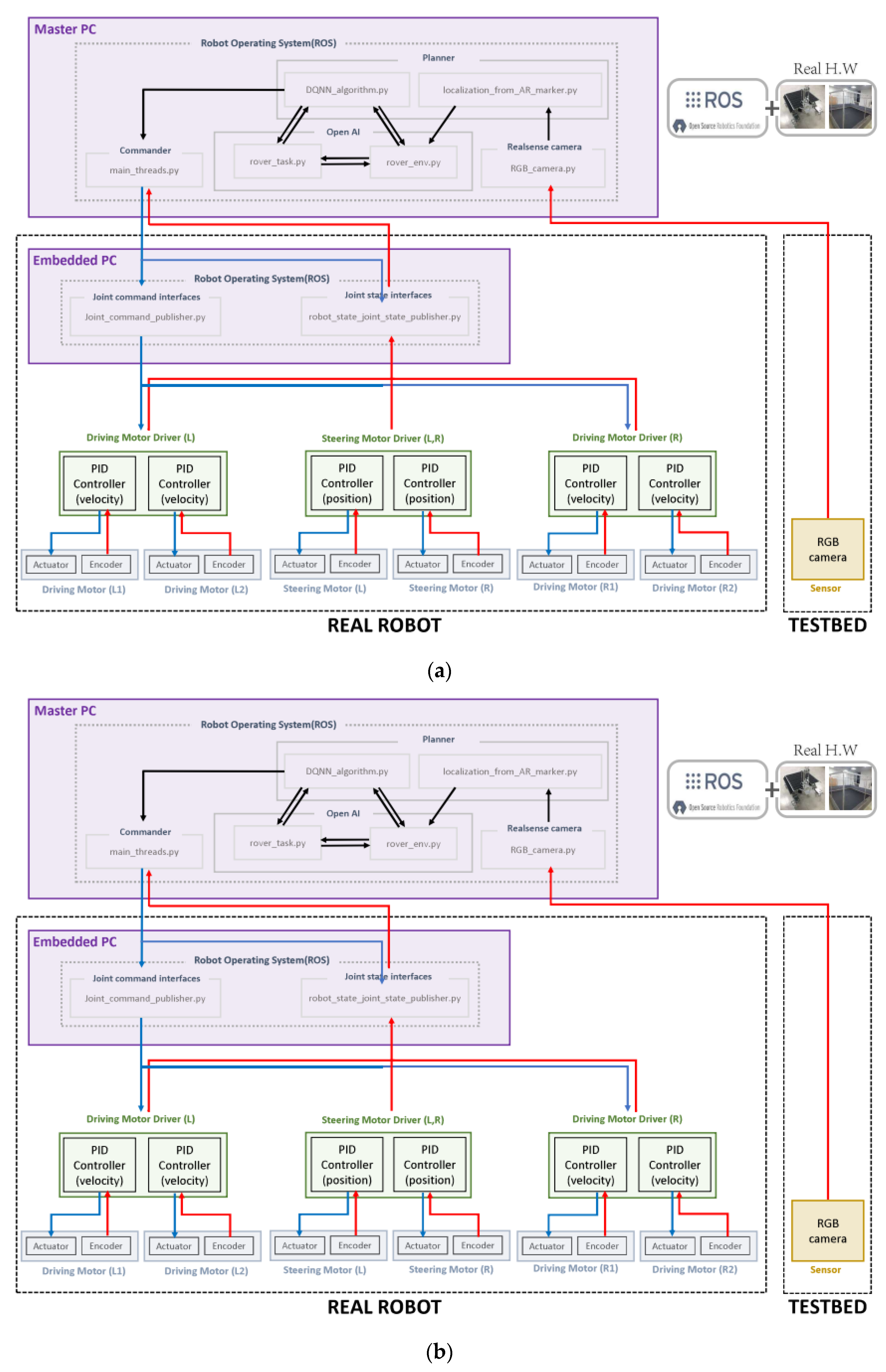
The control system of the actual robot was developed in the ROS Melodic [67], and Ubuntu 16.04 environment, as shown in Figure 17a. In this environment, detailed features, including motor control, data communication between the hardware interface and the embedded PC, and localization using RGB cameras (RealSense D435) and AR Marker, were implemented. The control system of the simulated robot model is presented in Figure 17b. The actual full-scale robot and the testbed were simulated as 3D models using Gazebo simulations [68]. A joint controller package with the same gear ratio as that of the actual robot was employed in the simulation model, replacing the encoder and motor driver. The robot’s localization data were obtained from the simulated testbed environment instead of using RGB cameras and an AR Marker. Here, the noise was intentionally included in the data.

4.2. Parameter Setup

In this paper, S ( 0 ,   0 ) and G ( 3000 ,   3000 ) were selected as the starting point and the target point, respectively, considering the actual dimensions of the testbed for the rover moving experiments. Meanwhile, boundary conditions were needed to determine whether each training episode was a success or a failure. If the agent took a certain action, and the resultant values of the five observation variables regarding the state of the rover were within these boundaries, the corresponding episode was considered to be still ongoing. Accordingly, rewards were given based on the three criteria, and the next action was then executed. In the meantime, when the state values affected by any actions of the agent were no longer within the boundaries, the corresponding episode was immediately terminated and then evaluated to be either a success or failure based on the final state values and boundary conditions. If even just one of the five observation variables was out of the boundary limit, the episode was considered to be a failure, and the corresponding cumulative reward was deducted. Then, the state of the robot was reset, and a new episode begun.
Finally, the thresholds λ , δ , and α needed to be adjusted. These parameters are directly related to the applied reward strategy, and critically affect the motion planning of the agent. The smaller these thresholds are, the longer the training takes, but it makes it possible to train the robot to perform more sophisticated motions. Figure 18 presents the setting margins for each criterion and the boundary conditions as the reset criterion. As discussed in 3.2.2 above, λ determines how closely the agent will approach the reference path. If r t is within this range, an even greater reward is given, and the size of the reward depends on the degree of closeness. Given that the width of the rover body is 300 mm, the threshold λ was set to 100 mm. δ represents how faithfully the agent follows the reference path. If θ e r r t is within this range, a greater reward is given. In this paper, this margin angle was set to ±10° to allow the robot to learn to perform motions while staying within the reference path. α is the threshold based on which the agent is considered to have reached the target point. If the final l t value of the agent is less than this threshold, the corresponding episode is finished. In this case, the episode is considered to be a success. The success radius α was set to 200 mm, about half of the total width of the robot, including the wheels.
As described in 3.2.2, the robot actions in the first experiment were composed of three discretized locomotion options. Figure 19a illustrates how the three inputs of the forward kinematics that are fixed at r g = 1001.6845   mm , w = 0.1531   rad / s , and v = 2.8571   cm / s are translated into a f o r w a r d , a l e f t , and a r i g h t , respectively, i.e., output actions in a normal state. Figure 19b shows how these three output motions differ in the case of a failure in the right steering motor of the robot, even though the same inputs as before are entered. The figure demonstrates how the red paths deviate from the original routes observed in a normal state when the robot makes turning actions. This is because the wheel slippage caused by the malfunction of the steering motor significantly affects the moving performance of the robot.
In the second experiment, the same test conditions were applied to compare the two different methodologies. Thus, the robot’s actions were constrained. Figure 20a shows that numerous action options may be produced as outputs of the forward kinematics depending on the angular velocity w . Only three output motions were allowed, as in the previous experiment, but the w value was continuous in the PID Path Follower, and this led to a difference in the moving speed of the rover when making turning actions. In order to ensure the same test conditions as in the first experiment, the radius of gyration r g was fixed at 1001.6845   mm , and the time per action step was set to 5   s . As can be seen in Figure 20b, the gyration radius of the rover was the same in all experiments.
Thus, although in the second experiment only three discretized steering motions were allowed in gyration, there can be numerous action options as outputs depending on the angular velocity. The yellow path is the trajectory of the rover in the case of a failure in the right steering motor, which differs from that in a normal state. When the control cycle is the same, this approach is more advantageous than the DQN in motion planning, thanks to its higher DOF with respect to the angular velocity. Except for that, all other test conditions were the same as in the first experiment.

4.3. Experimental Details and Results

The applicability of the DQN as a failure-safe motion planner for lunar rover control was verified by performing two sets of experiments in a virtual environment.
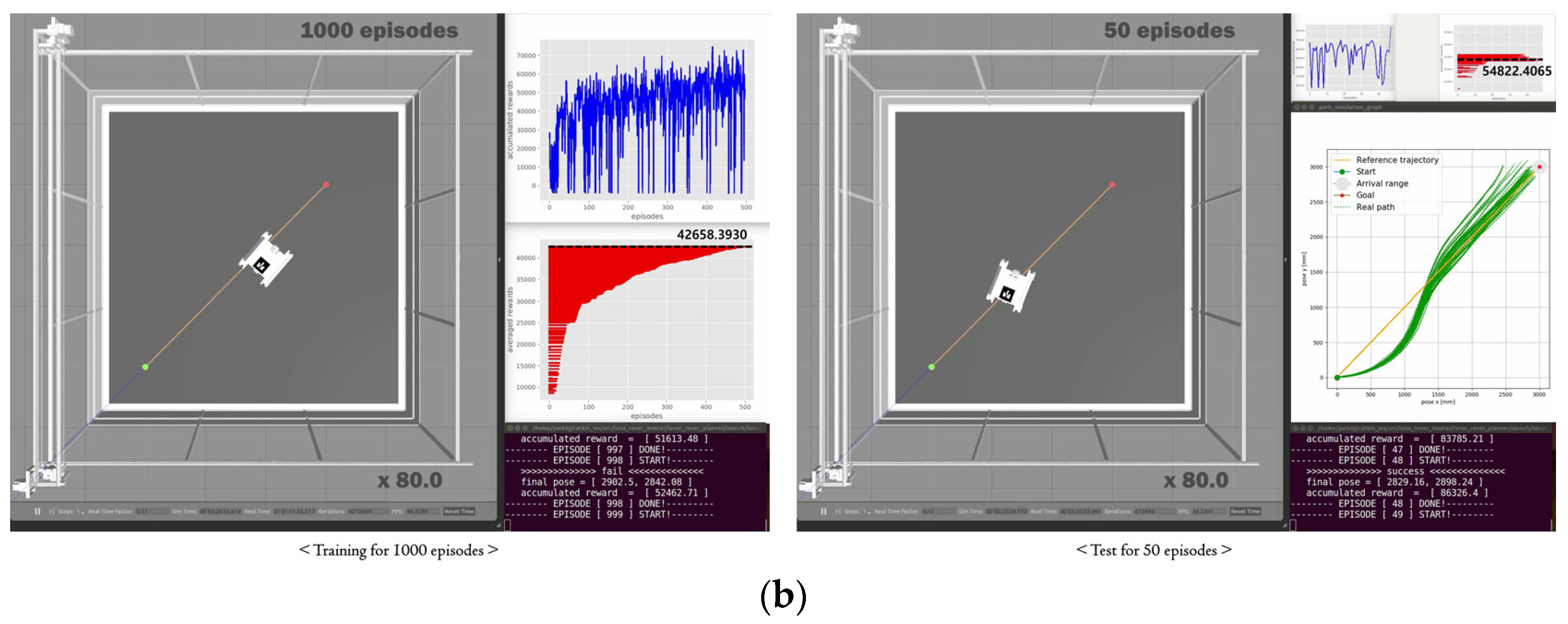
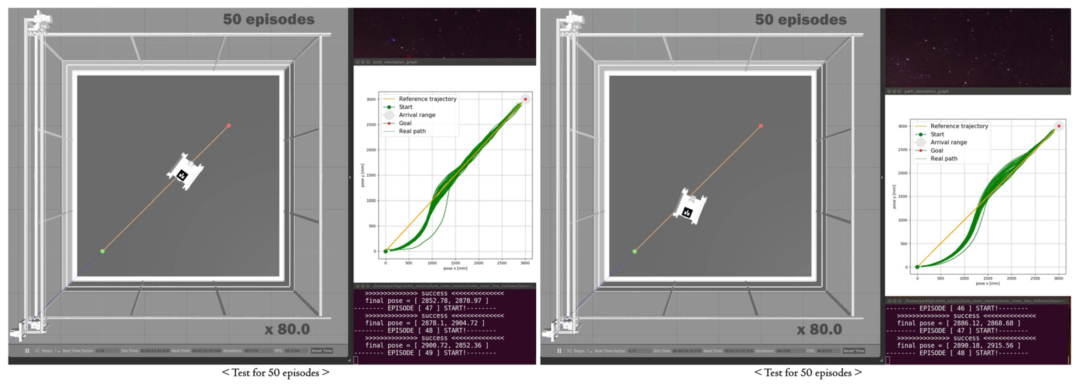
In the first experiment, the applicability of the failure-safe algorithm was evaluated, especially with respect to the mechanical unit of the lunar rover equipped with special steering mechanisms. The mission execution performance of the rover was evaluated based on three performance criteria, the success rate of reaching the target point, the ability to approach the optimum path, and the path-tracking ability, both in a normal state and when there was a failure in the right steering motor. In the normal state 500 training episodes were performed, and 1000 were performed for the steering motor, failure case, as shown in Figure 21a. A total of 50 test episodes were performed for normal and failure conditions, respectively, as shown in Figure 21b. The actual paths of the rover and the perpendicular position error from the optimum reference trajectory were repeatedly measured, and the averaged results were obtained, as shown in Figure 22.
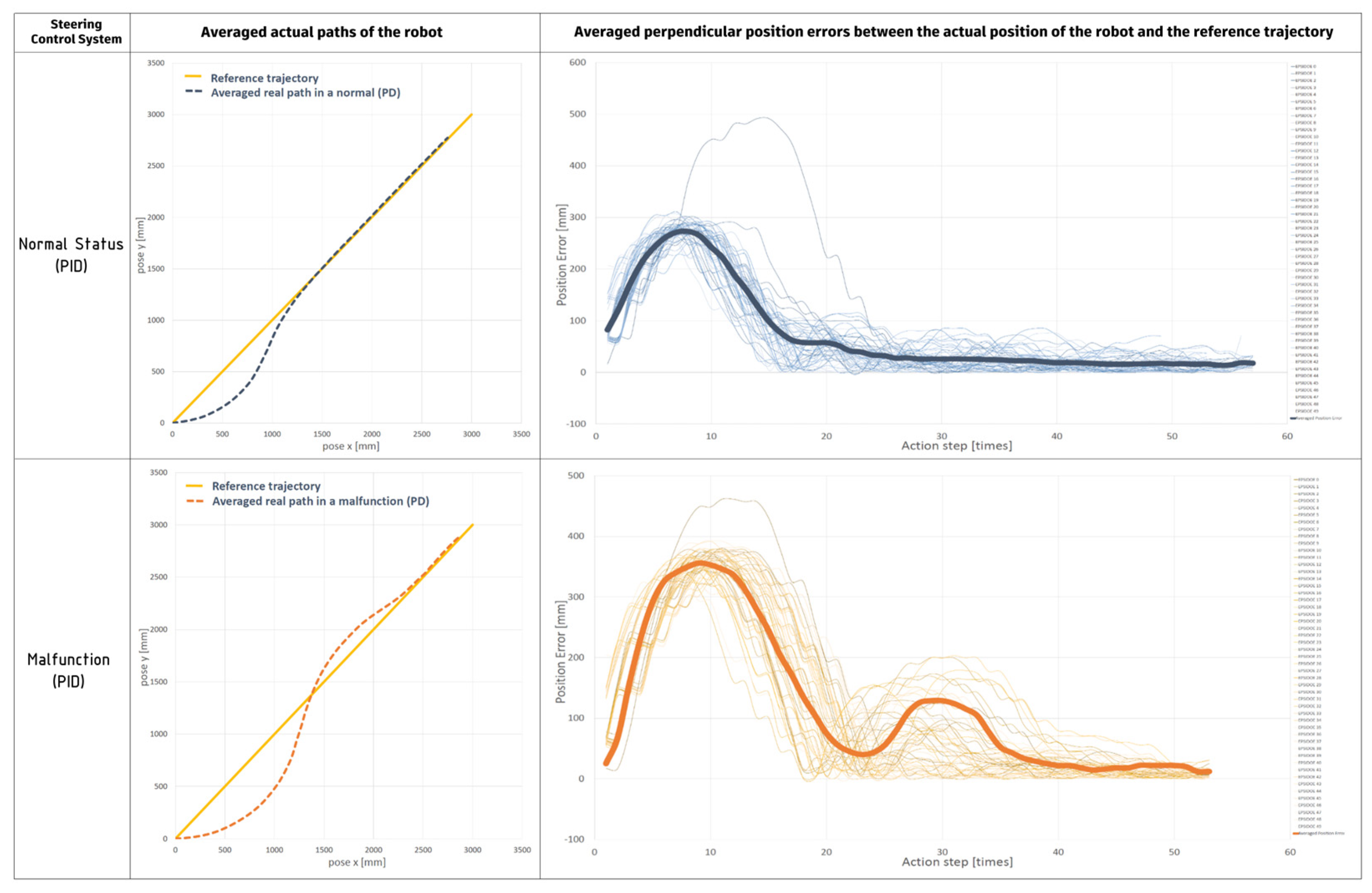
In the second experiment, the reliability of the failure-safe motion planning algorithm using the DQN was verified, especially with respect to linear paths given for each sequence of the Moon exploration missions. A PID controller-based tracking approach, among various conventional control methodologies, was employed as a comparison group, and their performance was assessed and compared based on three performance criteria. A PID controller tuned with optimal values was used, and 50 test episodes were performed in a normal state, while 50 test episodes were performed in the case of a failure in the steering motor in the same way as in the first experiment, as shown in Figure 23. Similarly, the averaged actual paths of the rover and the averaged perpendicular position errors between the actual position of the rover and the optimum reference trajectory were repeatedly measured, and the averaged results were obtained, as shown in Figure 24.

4.4. Applicability of the Failure-Safe Algorithm

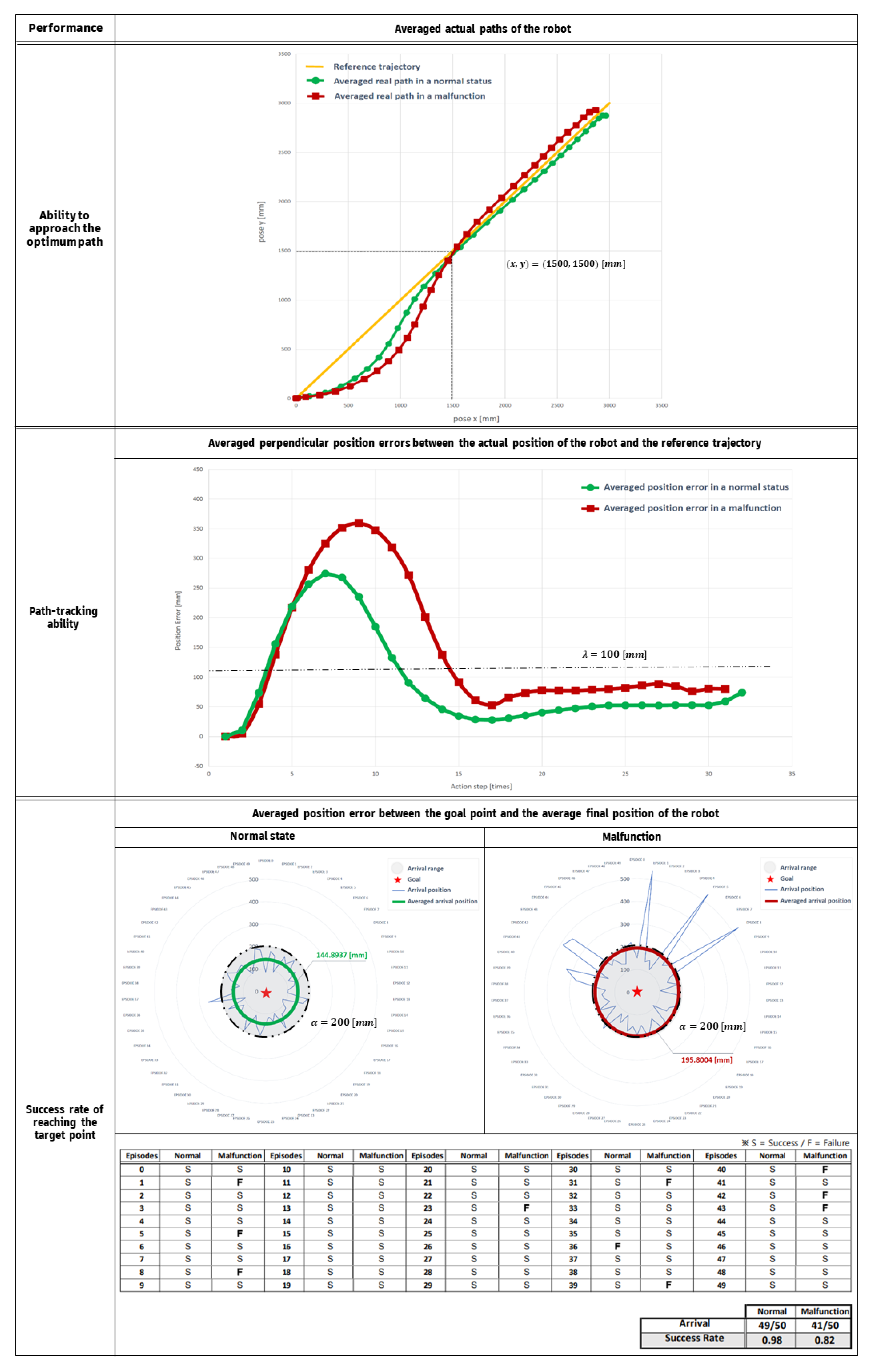
The results demonstrated that the DQN-based motion planning algorithm developed in this paper was applicable as a failure-safe solution for rover control in case of a failure in the steering motor. The detailed results are presented in Figure 25.
The averaged actual paths of the rover in the first experiment proved that there was no significant difference in its ability to approach the optimum path, between the normal and failure states. In both cases, when the rover approached the linear path, their initial coordinates were found to be similar to each other ( x = 1500.00   mm , y = 1500.00   mm ) .
The averaged perpendicular position errors between the actual position of the rover and the optimum reference trajectory were 50.00   mm in the normal state and 75.00   mm in the failure state, respectively. Despite the steering motor malfunction, the position error was less than 100.00   mm , the threshold λ . These results confirmed that its path-tracking performance was sufficiently high for the given mission.
Finally, the test for the success rate of reaching the target point was conducted 50 times in the normal and failure states, respectively. The last row of Figure 25 shows the detail. The success rate in a failure state was about 11.8279 % lower than that in a normal state relatively. However, although the total number of cases in which the rover arrived was lower due to the failure of the steering motor, the overall success rate still remained high, at 82.00 % . In addition, the position error between the target point and the average final position of the rover was 195.8004   mm in the failure state, but that figure was less than 200.00   mm , the threshold α , when the rover was considered to have reached the target point. These results also showed that the success rate of reaching the target point was also within the allowable range.

4.5. Reliability Comparison with a Conventional Control Method

The second experiment was performed to verify the reliability of the motion planner using the DQN, and the results were compared with those obtained from a conventional control method. In this paper, among various linear path-tracking methods, the PID Path Follower was employed as a comparison group thanks to its reliable control performance for a linear function, such as constant inputs.
The control loop of the PID Path Follower used in the experiment is presented in Figure 26. The controller receives data on the position error ( r t ) between the robot’s current position and the reference trajectory as a control input from the robot state calibrator. Subsequently, the controller adjusts the robot’s steering angular velocity w d on a 2D Cartesian coordinate system to minimize this position error. The PID Gain was set as follows: P = 0.2 , I = 0.0 , and D = 1.0 . These values were determined from repeated parameter tuning, which ensured that the 4-wheeled 2-steering lunar rover would exhibit its best performance as a mobile platform in a normal state.
The results of the second experiment showed that, in a normal state, the Path Follower based on the PID controller with optimized turning parameters was superior to the DQN-based motion planning method in terms of the ability to approach the optimum path and the path-tracking ability. However, when the steering motor failed, the robot approached the reference path at a later step ( x = 2500.00   mm , y = 2500.00   mm ) when the PID controller was used with the same parameters applied, as shown in the averaged actual paths of the robot. Furthermore, the position error between the current position of the rover and the reference trajectory exceeded the threshold λ , indicating that the path tracking had not been effectively performed in a reliable manner.
An overall comparison of the two methods is presented in Figure 27. The averaged actual paths of the robot in a failure state showed that the DQN-based motion planner allowed the robot to approach the reference trajectory relatively faster than the path follower using the PID controller. The perpendicular position errors between the current position of the rover and the optimum reference trajectory also verified the superiority of the DQN-based motion planner in path-tracking performance.
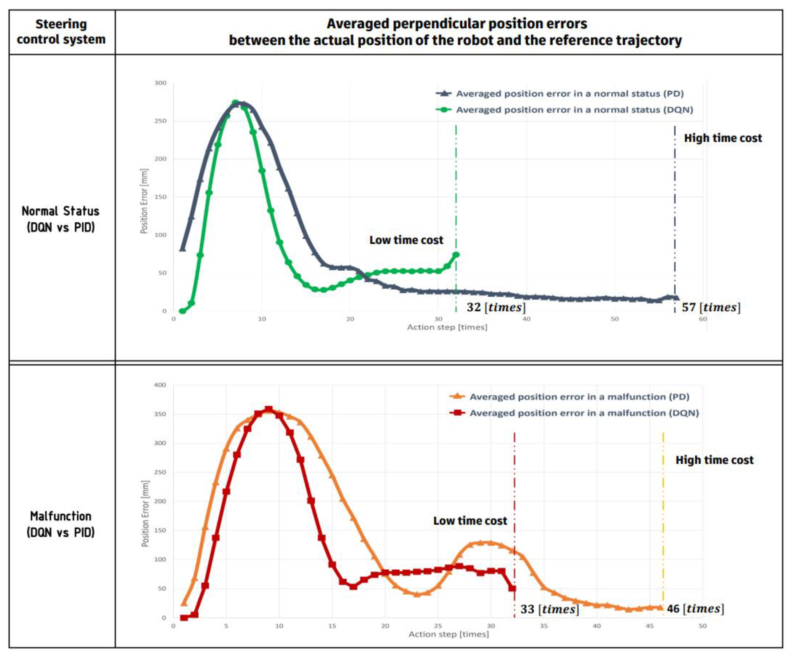
Further result analyses are presented in Figure 28. In the normal state, the number of steps required for the rover to reach the target point was 57   times for the PID controller and 32   times for the DQN-based motion planner, respectively. In the failure state, the figure was 46   times for the PID controller and 33   times for the DQN-based motion planner, respectively. Regardless of the steering motor failure, the DQN-based motion planner was found to be more efficient, requiring less time for the rover to arrive and, thus, reduced costs.
In summary, as previously discussed in Section 4.2, the path follower using the PID controller is considered to be more flexible for motion planning because it can produce numerous motion options with the steering angular velocity w . However, the DQN-based motion planner generally requires less time cost and is also superior, especially in a failure state, in terms of the ability to approach the optimum path and path-tracking ability.

5. Conclusions

In this paper, for a four-wheeled two-steering lunar rover, a deep reinforcement-learning-based failure-safe motion planning method has been studied. One of the characteristics of this mobile robot platform is that it is equipped with a modified explicit-steering mechanism. Four-wheeled lunar rovers have advantages in terms of compactness because they have fewer wheels, and better fit the limited space available in launch vehicles. The modified explicit-steering mechanism in this paper minimizes the number of actuators required, reducing the overall weight of the system. Furthermore, this mechanism allows rovers to have the robust structure for the Moon’s environmental conditions, with steering motors located inside the rover body. This paper proposed a reinforcement learning-based failure-safe motion planning algorithm to solve the critical mobility limitations issue in the non-holonomic four-wheeled rovers and uncertainty in rover control due to various environmental factors at play on the Moon’s surface. The proposed motion planning method combines the reinforcement learning approach with the robot’s kinematic model without the requirement for dynamics modeling such as a wheel–terrain interaction model. In addition, the failure-safe algorithm provides a safe motion planning strategy to ensure the execution of the rover’s mission even in the event of steering motor failure. To validate this method, simulations on high-slip flat terrain resulting from steering motor failure were demonstrated.
The experimental results obtained in this study confirmed that the proposed failure-safe algorithm exhibited comparable mission execution performance in a normal state and in the case of a failure in the steering motor. In the first experiment, the applicability of the failure-safe algorithm was validated. Especially, in the failure state, the overall success rate of reaching the target point was found to be high, at 82.00 % , and the position error between the target point and the average final position of the rover was 195.8004   mm while satisfying the threshold α of less than 200.00   mm . In addition, the ability to approach the optimum path was evaluated to be sufficiently high because the initial coordinates that the rover approached the reference path were comparable to that of the normal state ( x = 1500.00   mm , y = 1500.00   mm ) . The path-tracking ability was also suitable for the given mission, as the averaged perpendicular position errors were 75.00   mm and less than the threshold λ of 100.00   mm .
Meanwhile, it was also found that, in the case of a hardware failure, i.e., a steering motor malfunction, the Deep Q-learning Network was more reliable than a conventional control method for motion planning for the four-wheeled two-steering lunar rover. The second experiment was demonstrated to verify the reliability of the proposed motion planner, where the performance of the conventional path follower and the DQN-based motion planner was compared. The result showed that the DQN method’s performance was high in the case of a steering motor failure compared to the conventional control method. The ability to approach the optimum path was also relatively high in the proposed method, with a convergence point of ( x = 1500.00   mm , y = 1500.00   mm ) , while the conventional path follower’s point was at ( x = 2500.00   mm , y = 2500.00   mm ). The path-tracking ability of the conventional path follower was not enough to satisfy the condition as the position error between the current position of the rover and the reference trajectory exceed the threshold. Furthermore, it was additionally founded that the DQN-based motion planner required fewer steps for mission success in both normal and failure states than the conventional path follower. More specifically, the number of steps required for the rover to reach the target point was respectively 32   times in the normal state and 33   times in the failure state, which was less than the number of steps required by the conventional path follower. These results indicate that the proposed method reduced the time and cost required for the rover to arrive at its destination.
The reinforce learning-based failure-safe algorithm proposed as a motion planning solution for the four-wheeled two-steering lunar rover can be effectively employed in a failure state, but also used as a control system in a normal state by extending its applicability to include various ground types, such as rough or deformable terrains. A slippage-robust algorithm, a subject for future studies, can be applied to various ground conditions when it is difficult to predict the wheels’ slip behavior. With this level of scalability, the developed algorithm can be adopted as a flexible motion planning solution that effectively suits the unique conditions of each planet. In addition, this algorithm is valuable as a failure-safe solution for planetary exploration rovers, given the nature of this type of rover, i.e., difficult to maintain.

Author Contributions

B.-J.P. developed the methodology and implementations of the method and performed validations and obtained the results, and also contributed to the writing of the manuscript. H.-J.C. reviewed the manuscript. All authors have read and agreed to the published version of the manuscript.

Funding

This research was funded by the Ministry of Science, ICT and Future Planning (MSIP) under the space technology development program NRF-2016M1A3A9005563, supervised by the National Research Foundation of Korea (NRF). Also, this research was funded by the Korea Evaluation Institute of Industrial Technology (KEIT) funded by the Korea Government (MOTIE, Grant No. 20018216), Development of mobile intelligence SW for autonomous navigation of legged robots in dynamic and atypical environments for real application.

Institutional Review Board Statement

Not applicable.

Informed Consent Statement

Not applicable.

Data Availability Statement

Not applicable.

Acknowledgments

This work was supported in part by the Korea Evaluation Institute of Industrial Technology (KEIT) funded by the Korea Government (MOTIE) under Grant No. 20018216, Development of mobile intelligence SW for autonomous navigation of legged robots in dynamic and atypical environments for real application. The authors would also like to thank the Korea Institute of Science and Technology (KIST) for providing facilities and equipment.

Conflicts of Interest

The authors declare no conflict of interest.

References

  1. Schweitzer, L.; Jamal, H.; Jones, H.; Wettergreen, D.; Whittaker, W.L.R. Micro Rover Mission for Measuring Lunar Polar Ice. In Proceedings of the 2021 IEEE Aerospace Conference (50100), Online, 15 May 2021; pp. 1–13. [Google Scholar]
  2. Webster, C.; Reid, W. A Comparative Rover Mobility Evaluation for Traversing Permanently Shadowed Regions on the Moon. In Proceedings of the 2022 IEEE Aerospace Conference (AERO), Big Sky, MT, USA, 5–12 March 2022; pp. 1–15. [Google Scholar]
  3. Pavlov, C.A.; Rogg, A.; Johnson, A.M. Assessing Impact of Joint Actuator Failure on Lunar Rover Mobility. In Proceedings of the Lunar Surface Innovation Consortium (LSIC), El Paso, TX, USA, 2–3 November 2022. [Google Scholar]
  4. Seo, M.; Lee, W. Study on Mobility of Planetary Rovers and the Development of a Lunar Rover Prototype with Minimized Redundancy of Actuators. J. Korean Soc. Precis. Eng. 2019, 36, 339–348. [Google Scholar] [CrossRef]
  5. Niksirat, P.; Daca, A.; Skonieczny, K. The effects of reduced-gravity on planetary rover mobility. Int. J. Robot. Res. 2020, 39, 797–811. [Google Scholar] [CrossRef]
  6. Swinton, S.; McGookin, E. Fault Diagnosis for a Team of Planetary Rovers. In Proceedings of the 2022 UKACC 13th International Conference on Control (CONTROL), Plymouth, UK, 20–22 April 2022; pp. 94–99. [Google Scholar]
  7. Ono, M.; Rothrock, B.; Iwashita, Y.; Higa, S.; Timmaraju, V.; Sahnoune, S.; Qiu, D.; Islam, T.; Didier, A.; Laporte, C. Machine learning for planetary rovers. In Machine Learning for Planetary Science; Elsevier: Geneva, Switzerland, 2022; pp. 169–191. [Google Scholar]
  8. Gaines, D.; Doran, G.; Paton, M.; Rothrock, B.; Russino, J.; Mackey, R.; Anderson, R.; Francis, R.; Joswig, C.; Justice, H. Self-reliant rovers for increased mission productivity. J. Field Robot. 2020, 37, 1171–1196. [Google Scholar] [CrossRef]
  9. Ono, M.; Rothrock, B.; Otsu, K.; Higa, S.; Iwashita, Y.; Didier, A.; Islam, T.; Laporte, C.; Sun, V.; Stack, K. Maars: Machine learning-based analytics for automated rover systems. In Proceedings of the 2020 IEEE Aerospace Conference, Big Sky, MT, USA, 7–14 March 2020; pp. 1–17. [Google Scholar]
  10. Lätt, S.; Pajusalu, M.; Islam, Q.S.; Kägo, R.; Vellak, P.; Noorma, M. Converting an Industrial Autonomous Robot System into a Lunar Rover. 2020. Available online: https://www.researchgate.net/profile/Riho-Kaego/publication/351372661_Converting_an_Industrial_Autonomous_Robot_System_into_A_Lunar_Rover/links/609a397f92851c490fcee220/Converting-an-Industrial-Autonomous-Robot-System-into-A-Lunar-Rover.pdf (accessed on 18 December 2022).
  11. Blum, T.; Yoshida, K. PPMC RL training algorithm: Rough terrain intelligent robots through reinforcement learning. arXiv 2020, arXiv:2003.02655. [Google Scholar] [CrossRef]
  12. Rankin, A.; Maimone, M.; Biesiadecki, J.; Patel, N.; Levine, D.; Toupet, O. Driving curiosity: Mars rover mobility trends during the first seven years. In Proceedings of the 2020 IEEE Aerospace Conference, Big Sky, MT, USA, 7–14 March 2020; pp. 1–19. [Google Scholar]
  13. Gaines, D. Autonomy Challenges & Solutions for Planetary Rovers. 2021. Available online: https://trs.jpl.nasa.gov/bitstream/handle/2014/55511/CL%2321-3139.pdf?sequence=1 (accessed on 18 December 2022).
  14. Lojda, J.; Panek, R.; Kotasek, Z. Automatically-Designed Fault-Tolerant Systems: Failed Partitions Recovery. In Proceedings of the 2021 IEEE East-West Design & Test Symposium (EWDTS), Batumi, GE, USA, 10–13 September 2021; pp. 1–8. [Google Scholar]
  15. Vera, S.; Basset, M.; Khelladi, F. Fault tolerant longitudinal control of an over-actuated off-road vehicle. IFAC-Pap. Online 2022, 55, 813–818. [Google Scholar] [CrossRef]
  16. Sánchez-Ibáñez, J.R.; Pérez-Del-Pulgar, C.J.; Serón, J.; García-Cerezo, A. Optimal path planning using a continuous anisotropic model for navigation on irregular terrains. Intell. Serv. Robot. 2022, 1–14. [Google Scholar] [CrossRef]
  17. Hu, R.; Zhang, Y. Fast path planning for long-range planetary roving based on a hierarchical framework and deep reinforcement learning. Aerospace 2022, 9, 101. [Google Scholar] [CrossRef]
  18. Egan, R.; Göktogan, A.H. Deep Learning Based Terrain Classification for Traversability Analysis, Path Planning and Control of a Mars Rover. Available online: https://www.researchgate.net/profile/Ali-Goektogan/publication/356833048_Deep_Learning_based_Terrain_Classification_for_Traversability_Analysis_Path_Planning_and_Control_of_a_Mars_Rover/links/61af2bfdd3c8ae3fe3ed373c/Deep-Learning-based-Terrain-Classification-for-Traversability-Analysis-Path-Planning-and-Control-of-a-Mars-Rover.pdf (accessed on 18 December 2022).
  19. Blacker, P.C. Optimal Use of Machine Learning for Planetary Terrain Navigation. Ph.D. Thesis, University of Surrey, Guildford, UK, 2021. [Google Scholar] [CrossRef]
  20. Ugur, D.; Bebek, O. Fast and Efficient Terrain-Aware Motion Planning for Exploration Rovers. In Proceedings of the 2021 IEEE 17th International Conference on Automation Science and Engineering (CASE), Lyon, France, 23–27 August 2021; pp. 1561–1567. [Google Scholar]
  21. Tang, H.; Bai, C.; Guo, J. Optimal Path Planning of Planetary Rovers with Safety Considerable. In Proceedings of the 2021 International Conference on Autonomous Unmanned Systems (ICAUS 2021), Athens, Greece, 15–18 June 2021; pp. 3308–3320. [Google Scholar]
  22. Endo, M.; Ishigami, G. Active Traversability Learning via Risk-Aware Information Gathering for Planetary Exploration Rovers. IEEE Robot. Autom. Lett. 2022, 7, 11855–11862. [Google Scholar] [CrossRef]
  23. Zhang, J.; Xia, Y.; Shen, G. A novel learning-based global path planning algorithm for planetary rovers. Neurocomputing 2019, 361, 69–76. [Google Scholar] [CrossRef] [Green Version]
  24. Josef, S.; Degani, A. Deep reinforcement learning for safe local planning of a ground vehicle in unknown rough terrain. IEEE Robot. Autom. Lett. 2020, 5, 6748–6755. [Google Scholar] [CrossRef]
  25. Abcouwer, N.; Daftry, S.; del Sesto, T.; Toupet, O.; Ono, M.; Venkatraman, S.; Lanka, R.; Song, J.; Yue, Y. Machine learning based path planning for improved rover navigation. In Proceedings of the 2021 IEEE Aerospace Conference (50100), Online, 6–13 March 2021; pp. 1–9. [Google Scholar]
  26. Ding, L.; Gao, H.; Deng, Z.; Liu, Z. Slip-ratio-coordinated control of planetary exploration robots traversing over deformable rough terrain. In Proceedings of the 2010 IEEE/RSJ International Conference on Intelligent Robots and Systems, Taipei, Taiwan, 18–22 October 2010; pp. 4958–4963. [Google Scholar]
  27. Burke, M. Path-following control of a velocity constrained tracked vehicle incorporating adaptive slip estimation. In Proceedings of the 2012 IEEE International Conference on Robotics and Automation, St. Paul, MI, USA, 14–18 May 2012; pp. 97–102. [Google Scholar]
  28. Kim, J.; Lee, J. A kinematic-based rough terrain control for traction and energy saving of an exploration rover. In Proceedings of the 2016 IEEE/RSJ International Conference on Intelligent Robots and Systems (IROS), Daejeon, Korea, 9–14 October 2016; pp. 3595–3600. [Google Scholar]
  29. Inotsume, H.; Kubota, T.; Wettergreen, D. Robust path planning for slope traversing under uncertainty in slip prediction. IEEE Robot. Autom. Lett. 2020, 5, 3390–3397. [Google Scholar] [CrossRef]
  30. Sidek, N.; Sarkar, N. Dynamic modeling and control of nonholonomic mobile robot with lateral slip. In Proceedings of the Third International Conference on Systems (Icons 2008), Cancun, Mexico, 13–18 April 2008; pp. 35–40. [Google Scholar]
  31. Tian, Y.; Sidek, N.; Sarkar, N. Modeling and control of a nonholonomic wheeled mobile robot with wheel slip dynamics. In Proceedings of the 2009 IEEE Symposium on Computational Intelligence in Control and Automation, Nashville, TN, USA, 30 March–2 April 2009; pp. 7–14. [Google Scholar]
  32. Guo, J.; Li, W.; Ding, L.; Guo, T.; Gao, H.; Huang, B.; Deng, Z. High–slip wheel–terrain contact modelling for grouser–wheeled planetary rovers traversing on sandy terrains. Mech. Mach. Theory 2020, 153, 104032. [Google Scholar] [CrossRef]
  33. Zhang, W.; Lyu, S.; Xue, F.; Yao, C.; Zhu, Z.; Jia, Z. Predict the Rover Mobility Over Soft Terrain Using Articulated Wheeled Bevameter. IEEE Robot. Autom. Lett. 2022, 7, 12062–12069. [Google Scholar] [CrossRef]
  34. Li, S.; Ding, L.; Gao, H.; Chen, C.; Liu, Z.; Deng, Z. Adaptive neural network tracking control-based reinforcement learning for wheeled mobile robots with skidding and slipping. Neurocomputing 2018, 283, 20–30. [Google Scholar] [CrossRef]
  35. Farias, G.; Garcia, G.; Montenegro, G.; Fabregas, E.; Dormido-Canto, S.; Dormido, S. Reinforcement learning for position control problem of a mobile robot. IEEE Access 2020, 8, 152941–152951. [Google Scholar] [CrossRef]
  36. Gao, H.; Zhou, R.; Tomizuka, M.; Xu, Z. Reinforcement Learning Based Online Parameter Adaptation for Model Predictive Tracking Control Under Slippery Condition. In Proceedings of the 2022 American Control Conference (ACC), Atlanta, GE, USA, 8–10 June 2022; pp. 2675–2682. [Google Scholar]
  37. Basri, M.; Karapetyan, A.; Hassan, B.; Khonji, M.; Dias, J. A Hybrid Deep Learning Approach for Vehicle Wheel Slip Prediction in Off-Road Environments. In Proceedings of the 2022 IEEE International Symposium on Robotic and Sensors Environments (ROSE), Abu Dhabi, United Arab Emirates, 14–15 November 2022; pp. 1–7. [Google Scholar]
  38. Lopez-Arreguin, A.J.R.; Montenegro, S. Machine learning in planetary rovers: A survey of learning versus classical estimation methods in terramechanics for in situ exploration. J. Terramech. 2021, 97, 1–17. [Google Scholar] [CrossRef]
  39. Yu, X.; Wang, P.; Zhang, Z. Learning-based end-to-end path planning for lunar rovers with safety constraints. Sensors 2021, 21, 796. [Google Scholar] [CrossRef] [PubMed]
  40. Watkins, C.J.; Dayan, P. Q-learning. Mach. Learn. 1992, 8, 279–292. [Google Scholar] [CrossRef]
  41. Kober, J.; Bagnell, J.A.; Peters, J. Reinforcement learning in robotics: A survey. Int. J. Robot. Res. 2013, 32, 1238–1274. [Google Scholar] [CrossRef] [Green Version]
  42. Deisenroth, M.P.; Neumann, G.; Peters, J. A survey on policy search for robotics. Found. Trends Robot. 2013, 2, 1–142. [Google Scholar] [CrossRef] [Green Version]
  43. Ng, A.Y.; Jordan, M.I. PEGASUS: A policy search method for large MDPs and POMDPs. arXiv 2013, arXiv:1301.3878. [Google Scholar] [CrossRef]
  44. Van Hasselt, H.; Guez, A.; Silver, D. Deep reinforcement learning with double q-learning. In Proceedings of the AAAI Conference on Artificial Intelligence, Phoenix, AZ, USA, 12–17 February 2016. [Google Scholar]
  45. Polydoros, A.S.; Nalpantidis, L. Survey of model-based reinforcement learning: Applications on robotics. J. Intell. Robot. Syst. 2017, 86, 153–173. [Google Scholar] [CrossRef]
  46. Sun, H.; Zhang, W.; Yu, R.; Zhang, Y. Motion planning for mobile robots—Focusing on deep reinforcement learning: A systematic review. IEEE Access 2021, 9, 69061–69081. [Google Scholar] [CrossRef]
  47. Nishida, S.-I.; Wakabayashi, S. Analyses for mobility and control system of lunar rover. In Proceedings of the SICE Annual Conference 2010, Taipei, Taiwan, 18–21 August 2010; pp. 799–803. [Google Scholar]
  48. Luca, A.D.; Oriolo, G.; Samson, C. Feedback control of a nonholonomic car-like robot. In Robot Motion Planning and Control; Lecture Notes in Control and Information Sciences; 1998; Volume 229, pp. 171–253. Available online: https://link.springer.com/chapter/10.1007/BFb0036073 (accessed on 18 December 2022).
  49. Pepy, R.; Lambert, A.; Mounier, H. Path planning using a dynamic vehicle model. In Proceedings of the 2006 2nd International Conference on Information & Communication Technologies, Damascus, Syria, 24–28 April 2006; pp. 781–786. [Google Scholar]
  50. Kozłowski, K.; Pazderski, D. Modeling and control of a 4-wheel skid-steering mobile robot. Int. J. Appl. Math. Comput. Sci. 2004, 14, 477–496. [Google Scholar]
  51. Wang, D.; Qi, F. Trajectory planning for a four-wheel-steering vehicle. In Proceedings of the Proceedings 2001 ICRA. IEEE International Conference on Robotics and Automation (Cat. No. 01CH37164), Seoul, Korea, 21–26 May 2001; pp. 3320–3325. [Google Scholar]
  52. Laumond, J.P.; Sekhavat, S.; Lamiraux, F. Guidelines in nonholonomic motion planning for mobile robots. In Robot Motion Planning and Control; Laumond, J.P., Ed.; Springer: Berlin/Heidelberg, Germany, 1998; pp. 1–53. [Google Scholar]
  53. Tzafestas, S.G. Introduction to Mobile Robot Control; Elsevier: Geneva, Switzerland, 2013. [Google Scholar]
  54. Gonzalez, R.; Iagnemma, K. Slippage estimation and compensation for planetary exploration rovers. State of the art and future challenges. J. Field Robot. 2018, 35, 564–577. [Google Scholar] [CrossRef]
  55. Ishigami, G.; Nagatani, K.; Yoshida, K. Path planning for planetary exploration rovers and its evaluation based on wheel slip dynamics. In Proceedings of the Proceedings 2007 IEEE International Conference on Robotics and Automation, Rome, Italy, 10–14 April 2007; pp. 2361–2366. [Google Scholar]
  56. Bellman, R. Dynamic programming. Science 1966, 153, 34–37. [Google Scholar] [CrossRef]
  57. Mnih, V.; Badia, A.P.; Mirza, M.; Graves, A.; Lillicrap, T.; Harley, T.; Silver, D.; Kavukcuoglu, K. Asynchronous methods for deep reinforcement learning. In Proceedings of the International Conference on Machine Learning, New York, NY, USA, 19–24 June 2016; pp. 1928–1937. [Google Scholar]
  58. Theodorou, E.; Buchli, J.; Schaal, S. Reinforcement learning of motor skills in high dimensions: A path integral approach. In Proceedings of the 2010 IEEE International Conference on Robotics and Automation, Anchorage, AK, USA, 3–7 May 2010; pp. 2397–2403. [Google Scholar]
  59. Mnih, V.; Kavukcuoglu, K.; Silver, D.; Graves, A.; Antonoglou, I.; Wierstra, D.; Riedmiller, M. Playing atari with deep reinforcement learning. arXiv 2013, arXiv:1312.5602. [Google Scholar] [CrossRef]
  60. Kingma, D.P.; Ba, J. Adam: A method for stochastic optimization. arXiv 2014, arXiv:1412.6980. [Google Scholar] [CrossRef]
  61. Sutton, R.S.; Barto, A.G. Reinforcement Learning: An Introduction; MIT Press: Cambridge, MA, USA, 2018. [Google Scholar]
  62. Kormushev, P.; Calinon, S.; Caldwell, D.G. Reinforcement learning in robotics: Applications and real-world challenges. Robotics 2013, 2, 122–148. [Google Scholar] [CrossRef] [Green Version]
  63. March, J.G. Exploration and exploitation in organizational learning. Organ. Sci. 1991, 2, 71–87. [Google Scholar] [CrossRef]
  64. Chollet, F. Keras: The Python Deep Learning Library. Astrophysics Source Code Library, 2018. ascl: 1806.1022. Available online: https://keras.io/ (accessed on 18 December 2022).
  65. Brockman, G.; Cheung, V.; Pettersson, L.; Schneider, J.; Schulman, J.; Tang, J.; Zaremba, W. Openai gym. arXiv 2016, arXiv:1606.01540. [Google Scholar]
  66. Zamora, I.; Lopez, N.G.; Vilches, V.M.; Cordero, A.H. Extending the openai gym for robotics: A toolkit for reinforcement learning using ros and gazebo. arXiv 2016, arXiv:1608.05742. [Google Scholar]
  67. Quigley, M.; Conley, K.; Gerkey, B.; Faust, J.; Foote, T.; Leibs, J.; Wheeler, R.; Ng, A.Y. ROS: An open-source Robot Operating System. In Proceedings of the ICRA Workshop on Open Source Software, Kobe, Japan, 12–17 May 2009; p. 5. [Google Scholar]
  68. Koenig, N.; Howard, A. Design and use paradigms for gazebo, an open-source multi-robot simulator. In Proceedings of the 2004 IEEE/RSJ International Conference on Intelligent Robots and Systems (IROS) (IEEE Cat. No. 04CH37566), Sendai, Japan, 28 September–2 October 2004; pp. 2149–2154. [Google Scholar]
Figure 1. Steering mechanisms used for 4-wheeled mobile robots. (a) General explicit steering. (b) Car-like Ackermann steering. (c) Modified explicit steering. (d) Skid steering.
Aerospace 10 00219 g001
Figure 2. Driving and steering mechanisms of the 4-wheeled 2-steering lunar rover. (a) The dual-motor driving system with hardware redundancy. (b) The modified explicit-steering system, which requires software-level backup solutions. (c) Moving pattern of the rover with increased uncertainty in steering control due to a failure in the right steering motor.
Aerospace 10 00219 g002aAerospace 10 00219 g002b
Figure 3. Illustrations of 2D kinematic analysis when all motors work properly. (a) Pose of the robot in a 2D Cartesian coordinate system. (b) ICR of each wheel under the non-lateral slip condition. (c) Side view under the pure-rolling condition.
Aerospace 10 00219 g003
Figure 4. An illustration of the kinematic model ( r < 0 ) under the non-slip condition.
Aerospace 10 00219 g004
Figure 5. Illustrations of approximated kinematics modeling under the non-slip condition. (a) Modified explicit-steering mechanism. (b) Dual-motor driving mechanism.
Aerospace 10 00219 g005
Figure 6. Illustrations of 2D kinematic analysis when the right steering motor malfunctions. (a) Pose of the robot on a 2D Cartesian coordinate system. (b) ICR of each wheel under the lateral slip condition. (c) Side view under the longitudinal slip condition.
Aerospace 10 00219 g006
Figure 7. Slip dynamics when the right steering motor malfunctions. (a) Changes in the rotation center point position of each wheel due to slippage. (b) Change in the center point position of the robot body due to the slip of each wheel, and its recursive effect, causing further slip to occur in the four wheels.
Aerospace 10 00219 g007
Figure 8. Rover motions required by sequence-based commands for a Moon exploration mission.
Aerospace 10 00219 g008
Figure 9. Controllability achieved by model-free learning during whole dynamics model-free control.
Aerospace 10 00219 g009
Figure 10. Classification of reinforcement learning approaches.
Aerospace 10 00219 g010
Figure 11. An illustration of the Deep Q-learning Network (DQN).
Aerospace 10 00219 g011
Figure 12. A view of the rover projected on a 2D Cartesian coordinate system as observed from the Moon’s orbit.
Aerospace 10 00219 g012
Figure 13. Reference path, along with the state values and constant thresholds used for reward discrimination.
Aerospace 10 00219 g013
Figure 14. Reward discrimination table describing step rewards per action r e w a r d S .
Aerospace 10 00219 g014
Figure 15. Failure case categorization of the seven discrete angle ranges in the rover’s right steering motor failure.
Aerospace 10 00219 g015
Figure 16. Images of the full-scale robot and testbed environment, and simulated models reflecting their actual physical characteristics.
Aerospace 10 00219 g016
Figure 17. A schematic of the control system of the 4-wheeled 2-steering lunar rover. (a) Simulated robot system implemented based on the actual hardware interface. (b) Robot system implemented in a simulation environment.
Aerospace 10 00219 g017
Figure 18. Experimental parameter setting for training and test episodes.
Aerospace 10 00219 g018
Figure 19. Approximated forward kinematics used for rover locomotion control in the DQN. (a) Parameter setting input to define three fixed actions. (b) Gyration paths for the rover’s three actions in a normal state (upper) and in steering motor malfunction (lower).
Aerospace 10 00219 g019
Figure 20. Approximated forward kinematics used for rover locomotion control in the PID. (a) Input parameter setting to define actions. (b) Gyration paths for the rover’s three steering motions in a normal state (upper) and in steering motor malfunction (lower).
Aerospace 10 00219 g020
Figure 21. Training episodes (left) and test episodes (right) performed in the respective environments. (a) 500 training episodes and 50 test episodes performed in a normal state. (b) 1000 training episodes and 50 test episodes performed for the right steering motor failure case.
Aerospace 10 00219 g021aAerospace 10 00219 g021b
Figure 22. Averaged actual paths and perpendicular position error from the optimum reference trajectory obtained through repeated experiments on motion planning with the DQN.
Aerospace 10 00219 g022
Figure 23. 50 test episodes performed in a normal state (left) and 50 test episodes performed in the case of a failure in the right steering motor (right).
Aerospace 10 00219 g023
Figure 24. Averaged actual paths and perpendicular position error from the optimum reference trajectory obtained through repeated experiments in motion planning with the PID controller.
Aerospace 10 00219 g024
Figure 25. Quantitative analyses based on three performance criteria (thresholds) in motion planning with the DQN.
Aerospace 10 00219 g025
Figure 26. Control loop of the path follower based on the PID controller.
Aerospace 10 00219 g026
Figure 27. Reliability analysis of the two motion planning methods (PID and DQN), both in a normal state and in the case of a failure in the steering motor.
Aerospace 10 00219 g027
Figure 28. Time cost analysis of the two motion planning methods (PID and DQN) with respect to the average number of action steps required for the rover to reach the target point.
Aerospace 10 00219 g028
Disclaimer/Publisher’s Note: The statements, opinions and data contained in all publications are solely those of the individual author(s) and contributor(s) and not of MDPI and/or the editor(s). MDPI and/or the editor(s) disclaim responsibility for any injury to people or property resulting from any ideas, methods, instructions or products referred to in the content.