Abstract
Using the unsteady vortex lattice method based on the potential flow theory, a rapid modeling approach is developed for the aerodynamic computation of multi-lifting surfaces. Multiple lifting surfaces with different geometric parameters and grid divisions can be quickly integrated and meshed with the object-oriented data structure. The physical influence between different lifting surfaces was modeled, and the wake–surface interaction was also considered by using different built-in vortex core models. The trajectory data were used to replace the pre-calculated downwash superposition for boundary condition integration, and the instantaneous boundary condition was generated directly from the kinematic states and mesh messages of the model concerned. Considering the direct coupling effect between aerodynamics and rigid body dynamics, the function for free flight was built for medium-fidelity dynamic simulations and aerodynamic data identifications. The proposed high-efficiency modeling and simulation process can be easily applied to models with any number of different lifting surfaces and arbitrary motion modes.
1. Introduction
With the development of the aviation industry, various unmanned aerial vehicles (UAVs) are widely used in different fields, and their designs are constantly updated. The estimation of aerodynamic forces is very important in the preliminary design process of UAVs. Based on the aerodynamic loads at different flight conditions, it is possible to evaluate the driving force required for a wing morphing mechanism [1], predict the stress of the wing’s internal structure [2], and analyze the aeroelastic response of the wing [3]. In addition, in order to evaluate the aircraft stability and performance and design flight controllers, it is required to develop a high-fidelity flight dynamics model, for which aerodynamic data are an essential part. Aerodynamic parameters can generally be obtained through wind tunnel tests, flight tests, or computational fluid dynamic (CFD) simulations. Among them, the wind-tunnel-based method is widely used to measure the aerodynamic characteristics, but it is limited by the costs. Flight tests are usually conducted to verify and update the aerodynamic model obtained by wind tunnel tests and numerical calculations, but they are seldom performed at the aircraft design stage. With the development of software and hardware for numerical simulations, the CFD-based method has attracted greater attention. However, it is not computationally efficient to obtain the complete aerodynamic data when applied to models with a large number of cells in the flow field grid [4].
To improve the computational efficiency of numerical methods at the stage of aircraft conceptual and preliminary design, the potential flow theory has been thoroughly studied, which involves the solution of Laplace’s equation satisfied by the velocity potential [5]. The differential equation is discretized into algebraic equations by using different singularity elements. As a steady-state aerodynamic computation method established early in the 1970s, the vortex lattice method (VLM) has been verified and further developed in engineering applications [6,7,8]. It plays an important role in the calculation of the aerodynamic characteristics of fixed-wing aircraft. For the unsteady field, the doublet lattice method (DLM) has been developed, in which the doublet lattice can replace the original vortex grid in the VLM to calculate the unsteady aerodynamic forces under simple harmonic vibrations [9]. It has also become a powerful tool for aeroelastic analysis of subsonic aircraft [10]. However, as a linear method that is limited to simple motions with small deformations along the normal direction of each wing panel, the DLM cannot deal with the aircraft with complex geometric shapes, large deformations, or irregular motion states. There have been other unsteady-state aerodynamic computation methods developed, for instance the strip theory [11], which also has similar limitations due to the simplification of the modeling.
The unsteady vortex lattice method (UVLM) is a direct extension of the VLM from the steady to unsteady conditions. It inherits the characteristics that the VLM is suitable for aerodynamic modeling of aircraft with complex geometries, and thus, it can be used to model nonlinear effects, such as the shedding of the wake. Since the pioneering works on the methodology’s development [12,13], the UVLM has been broadly applied to various problems, including the aerodynamic calculation of rotary wings [14,15], flutter suppression of flexible wings [16,17], gust mitigation of high altitude long-endurance wings [18], and multidisciplinary optimization of the overall design [19]. Because the interaction among wing components can be considered, the UVLM can achieve a quite good fidelity, which makes it a preferred method in the aerodynamic calculation of morphing aircraft. For the morphing UAV, when the deformation of the wing is so slow that the resulting unsteady effects contribute little to the total aerodynamic force, it is considered acceptable not to use the unsteady wake model [20]. Under the assumption of a large deformation rate, the accuracy of the solution can be improved by establishing the unsteady wake vortex [21]. Moreover, the UVLM is a time domain method and can capture arbitrary responses. This makes it more convenient to consider the coupling effect of the deformation caused by the flexibility of the wing structure [22]. Typical applications include the aeroelastic stability analysis of flexible aircraft with large-aspect-ratio wings [23,24], the prediction of the rotor loads of a wind turbine [25,26], as well as the modeling of the flapping wings of insects [27,28].
Besides sorts of CFD software packages using the finite-volume method or finite-element method [29], there is some software developed based on the VLM for steady potential flow, such as AVL [30], Tornado [31,32], and XFLR5 [33], providing friendly aerodynamic calculation environments for individual researchers. In further consideration of the effect of unsteady flow and its dynamic coupling with the beam structure, SHARPy gives a powerful modeling function for very flexible aircraft and turbines with slender geometric profiles [34]. Due to the superiority of its computational efficiency, the UVLM has more possibilities for engineering applications. In this paper, a tool for aerodynamic modeling and simulation of multiple lifting surfaces is developed based on the UVLM [35]. Below is a brief summary of the features of the proposed method:
- Based on the idea of object-oriented programming, the mesh generation and part assembling for an arbitrary number of lifting surfaces can be easily performed as every surface can be defined as an object instance of the class to be quickly integrated into the model.
- The physical influence between multiple lifting surfaces is considered in the modeling process. With different built-in vortex core models, the wake–boundary interaction is also included to expand this tool to more engineering applications.
- Boundary conditions are directly updated based on the dynamic mesh, which can be used to model complex motions.
- Inspired by the concept of free flight, this tool generates not only the aerodynamic state-space data based on the frozen wake assumption, but also the six-degree-of-freedom (6DOF) rigid-body dynamics model. Nonlinear time domain simulations can be directly conducted using this integrated model, which gives a higher-fidelity flight simulation with the consideration of unsteady effects.
- The technique of parallel programming is utilized to improve the calculation performance of the problems involving large wakes. This makes it possible to efficiently conduct the modeling and simulation on a personal computer.
The rest of this paper is organized as follows. Section 2 introduces the basic theoretical background and formulation of the UVLM. Then, the modeling process for multi-lifting surfaces and the details of the algorithm implementation are presented in Section 3. The proposed modeling and simulation tool is tested in Section 4 using benchmark problems and practical engineering applications. Finally, Section 5 concludes the paper.
2. UVLM Formulation
2.1. Basic Concepts of Potential Theory
The UVLM is derived from potential theory [35]. With the irrotational incompressible inviscid flow assumption, the velocity potential is defined to represent the velocity distribution of the flow field, and the velocity at each point can be obtained as its gradient:
The governing equations (Navier–Stokes equations) of fluid are reduced to Laplace’s equation, and it can be written in Cartesian coordinates as
As can be seen, the linearity of the velocity potential is particularly important so that the entire flow field can be expressed as a superposition of a series of fundamental solutions as
There are two boundary conditions. The first one states that the flow cannot penetrate the solid boundary, that is the velocity vector must be tangent to the lifting surface:
where is the lifting surface’s velocity and is the unit vector normal to the lifting surface. The unsteady effect is introduced here since both and may be time-dependent. The second boundary condition requires that the flow disturbance caused by the surface motion diminish at infinity:
where . In addition, the streamwise strength of the vorticity shed into the wake can be determined by Kelvin’s circulation theorem, which states that the circulation around a fluid curve enclosing the wing and its wake remains constant with time:
In the numerical solution of the actual flow field that satisfies the potential flow theory, the key issue is to select an appropriate basic solution form to construct the entire flow field and boundary conditions.
2.2. Vortex Element
In the UVLM, vortex rings are chosen as fundamental solutions to construct the flow field that satisfies the basic equation. To model aircraft wings or other lifting surfaces suitable for thin wing theory, the mean surface of the wing can be discretized using rectangular or trapezoidal elements. According to the Biot–Savart law, the velocity induced by an infinitesimal piece of the vortex filament with the circulation as shown in Figure 1 can be written as
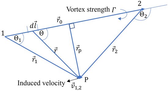
Figure 1.
The sketch of a vortex segment.
The integration of Equation (7) can be used to calculate the velocity induced by a finite-length vortex segment at any point, as presented in Figure 1.
For the lifting surface satisfying the thin wing theory, a group of vortex rings can be used to formulate the whole flow field. As sketched in Figure 2, a vortex lattice consists of four vortex vectors connected head to tail. The boundary vortex elements are arranged to fit the whole lifting surface. A finite number of rows of wake vortex elements are predefined behind the trailing edge of the lifting surface to simulate the wake shedding process.
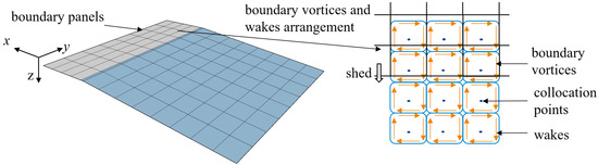
Figure 2.
The sketch of the vortex ring elements.
The boundary conditions are enforced at the collocation points, which are placed at the three-quarter chord of each boundary vortex, as shown in Figure 2. The zero normal flow boundary condition imposes that the superposition of the influences of all boundary vortices and wakes equals the flow normal to the panel at the collocation points. Because the geometric parameters are known, the boundary condition can be rewritten as
where and are the aerodynamic influence coefficient matrices corresponding to the velocity at the collocation points induced by boundary vortices and wakes, respectively. on the right side of the above equation represents the component of local flow in the normal direction of the panel at the collocation points. The local normal flow at the collocation point of panel k can be integrated as follows:
where the subscript k is the identical number of elements and collocation points, is the far field velocity, is the relative velocity due to the geometric deformation and it can be calculated by interpolating the relative velocities of the corner points of the element, is the disturbance flow velocity to consider the influence of gusts, and is the velocity contributed by the boundary rotations.
2.3. Wake Transport
Previous subsections introduced the discretization process in space. For the steady case, the wake location can be predefined according to the inflow velocity, and the vortex strength of all boundary vortices and wakes can be solved by integrating Equations (9) and (10). It should be noted that, if a wake vortex element is shed from the trailing edge, its strength will be conserved. This conforms to the Helmholtz theorems, which imply that there is no vortex decay [36], and the uniqueness of the solution of algebraic equations is guaranteed at the same time. Therefore, in the steady-state VLM method, the same result can be obtained by using the horseshoe vortex to model the wakes. In order to consider the wake convective process and the relative unsteady effects, we need to further perform the discretization in the time domain. The first-order explicit time-stepping scheme is used to capture the feature of the physical process. With a time-stepping form, the wake convection at time step n can be written as
where the superscripts n and represent the nth and the th time step and the subscripts b and w represent the boundary vortex element and the wall element. With this definition of the notation, and are the vertex coordinates of the wake and boundary vortex elements, respectively. and are constant matrices determined by the vortex and wake element arrangement, where is used to assign the coordinates of the trailing edge boundary vortex nodes to the first-row wake nodes and is used to shift the other wakes in the flow direction. The new position from the second row to the last row is derived by adding the last term on the right-hand side, the displacement of these wakes due to induced velocity and relative velocity at the current time step.
2.4. Vortex Core Model
The wake shedding from the trailing edge will move with the local velocity, and thus, wake–surface interaction is inevitable. When the distance between the vortex line and the control point is infinitely small, a singularity will happen when calculating the induced velocity according to Equation (8). The vortex core model is introduced to avoid the singularity in the numerical calculation. Moreover, through the expansion of the wake vortex model, the effect of viscosity can be partly considered.
As shown in Figure 3a, inside the vortex core, the velocity of the tangential flow should be close to zero instead of infinity, as represented by Equations (7) and (8). For a finite-length segment, the simplest way to avoid the singularity is a vortex core cutoff by assuming that the self-induced velocity inside the vortex core is zero. The Scully model [37] is a typical example for considering the viscosity correction, as shown in Figure 3b, and the velocity distribution for a finite vortex line in this model is
where is the Oseen parameter. is the core growth rate of the wake, and it is usually affected by the Reynolds number. As the viscosity effect is introduced by the kinematic viscosity , the vortex core diameter changes with time. For the Scully model and other similar vortex core models, the induced velocity calculation can be integrated as a subroutine for program implementation as
where the arguments represent the location of Points 1, 2, and P in Figure 1, respectively. The built-in vortex core model can be used in various scenarios with different values of the model index argument .
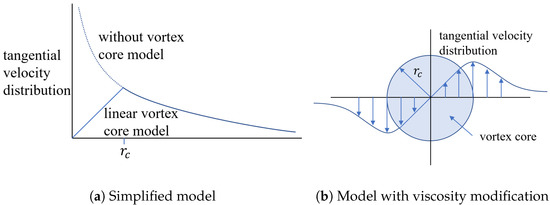
Figure 3.
Velocity distribution around a vortex core.
2.5. Aerodynamic Force
After the vortex strength is solved by Equations (2) and (4), the aerodynamic forces can be calculated according to Joukowski method [38]. The aerodynamic force at the midpoint of each vortex segment consists of the steady part and the unsteady part .
where is the local flow velocity, is the increment of the vortex vector, is a unit vector describing the direction of the local flow velocity, and the scalar c is the length of the vortex segment. In practical applications, it is not necessary to calculate the aerodynamic forces for all vortex segments of each vortex element. The effective vortex strength is introduced, and the calculation of the aerodynamic force on element k can be written as
where is the element area, is the unit normal vector of the vortex ring, and is the effective vortex strength.
2.6. State-Space and Time-Stepping Forms
The state-space form of the UVLM is the linearization of the model at a specific state, and it can be used to represent the aerodynamic force of the model near that state. There is a relationship between discrete state-space and time-stepping forms. However, there are no grid changes in the state-space form of the UVLM because the influence matrices are constant for a specified linearization point. Rewriting the Helmholtz theorem in Equation (11) without considering the update of the grid position [35],
Based on the forward Euler method, the derivative of the vortex strength with respect to time is replaced by the difference, and the change rate of the vortex strength can be expressed as follows:
The continuous aerodynamic model in the state-space form can be easily obtained as a byproduct of the modeling process after the influence matrices are calculated [39]. It can reflect the unsteady effect around the modeling condition. By considering the boundary and nonlinear wake updating, the time-stepping form has higher fidelity and can be used in flight simulations more conveniently without interpolations.
3. Modeling Process and Algorithm Implementation
3.1. Geometry Discretization
In this section, the UVLM is applied to model the aerodynamics of multi-lifting surfaces. The first step of the modeling process is geometry discretization. The smallest discrete unit is the surface object. To consider the camber of the lifting surface, the airfoil is also set as an argument of the node and element generation function. The camber line is automatically generated through a fitting and interpolation function according to the standard airfoil data. As shown in Figure 4, with the geometric characteristics given by the attributes of the surface object and airfoil fitting, the grid generation can be performed quickly and controlled conveniently by the grid seeding parameters. After the grid and nodes’ information is obtained, the information on the relative boundary vortex elements and nodes is generated. For more complex curve and facet modeling, the parameters of the elements and nodes can be loaded from other tools. The wake vortices are generated over time according to the movement of the lifting surface. In order to avoid using dynamic arrays, the memory is preallocated by prescribing the wake with zero vortex strength. Different from the boundary vortex, to apply the vortex model including the viscosity modification, a parameter named the wake age is used to mark the period from shedding to the current time step.
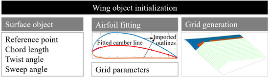
Figure 4.
The process of geometry discretization of a wing object.
As shown in Figure 5, for an object with multiple lifting surfaces such as aircraft with conventional configurations, an upper class with the name of the aircraft is defined. An array containing all single-surface objects is used to reconstruct a new wing object in the aircraft object initialization process.
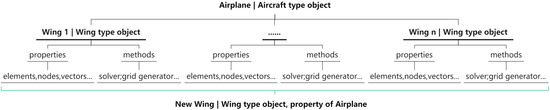
Figure 5.
The data structure defined for modeling of multi-lifting surfaces.
3.2. Boundary Condition Integration with Kinematic States
In the boundary condition integration process, different motion modes are often converted to different downwashes applied to a static discretized element model. There is no doubt that, no matter how complex the motion mode is, the boundary condition can be derived from the relative movement relationship between the body coordinate system and the Earth coordinate system. However, the wake update process cannot be easily performed when considering the motion including the translation and rotation in different directions at the same time. A simple illustration of a two-dimensional plate pitch oscillation case is shown in Figure 6, where the wakes on the moving boundary and static boundary are obtained based on the trailing edge path and the relative wind speed, respectively. It can be observed that the relative positions between the wake and the plate for moving and static boundaries are obviously different. Compared with the static boundary with relative wind velocity, the moving boundary can reflect the physical processes of lifting surfaces’ motion and vortex shedding more accurately.
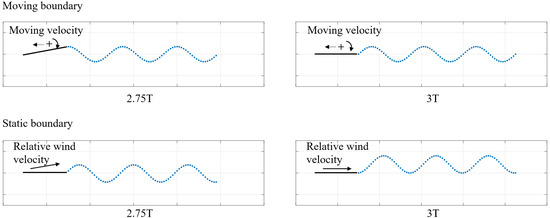
Figure 6.
Comparison of moving and static boundaries.
For more convenient and flexible boundary condition integration, the kinematic states of the flight dynamics are introduced to simulate the real flight process. The state variables include , the components of the velocity and angular rate in the body frame, and X, Y, Z, , the components of the position and attitude in the Earth frame of every surface. The normal velocity calculation for boundary integration can be rearranged as a function:
When the trajectory of lifting surfaces is given, the modeling of wake shedding is an intuitive process. The new corner points of the wake are generated at the location of the last row boundary vortex nodes and then move with the disturbance and induced velocities in the subsequent time steps. The coordinates of the wake vertices can be calculated using Equation (22), given below. Compared with Equation (11), using Equation (22) can avoid errors caused by the calculation of the wake position based on for nonlinear motions.
A public class is defined to record the components of velocity, angular rate, position, and attitude. For a system with multiple lifting surfaces, every surface has such a type of attribute to store its own kinematic states. A prescribed trajectory can be easily represented by a group of arrays with the predefined independent states and time as the indices. In addition to the simulation of arbitrary motions, the arrays can also be extended to include extra information and used to simulate the in-flight morphing and the multi-aircraft formation flight.
3.3. Dynamic Coupling
For conventional aerodynamic numerical calculations, the predefined boundary condition is used to obtain the loads or aerodynamic coefficients needed for the dynamic simulation. However, in real engineering applications, the aerodynamic forces are usually coupled with rigid body dynamics. If only using the linearized or interpolated aerodynamic state-space data, it does not make full use of the power of the UVLM in unsteady aerodynamic modeling. The idea of the time-stepping form combined with rigid body dynamics coupling was implemented to make better use of the characteristics of the UVLM. It can avoid the loss of accuracy caused by the interpolation and linearization processes of aerodynamic data. The 6DOF nonlinear dynamic model of a rigid body can be expressed as
where is the vector composed of the velocity, attitude, and position variables of the rigid body. is the input vector, containing the contributions of the aerodynamic forces and thrusts. As shown in Figure 7, different from the state-space form, which is fixed at linearized points, the grid is updated at every time step in the aerodynamic solver with the kinematic states input from the 6DOF dynamic solver. Similarly, the 6DOF dynamic solver is called at every time step with the forces and moments input from the aerodynamic solver. For different applications with different reduced frequency ranges, the time step of the 6DOF dynamic solver can be adjusted properly to ensure the time step matching and the dynamic solution accuracy. More details about 6DOF rigid body dynamics modeling and calculation can be found in the related reference books [40].
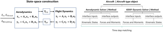
Figure 7.
The illustration of the dynamic coupling using the state-space model (left) and the time-stepping model (right).
3.4. Algorithm and Data Structure
The main feature of the algorithm was described in the previous section, and here, the detailed flow chart of the algorithm is shown in Figure 8. According to the imported information on the geometric and grid parameters, the initialization of Process 1 and Process 2 is first performed. All the elements, nodes, and relative vectors are generated at this step. Then, in Process 3, the influence matrices are calculated, and the aerodynamic state-space matrices can be derived based on the given linearization condition and the prescribed wake. Actually, the state-space data can also be exported at any time step to represent the instantaneous motion state and wake shape. The loop of time stepping is defined by Processes 4 to 6. If the direct dynamic coupling is considered, the boundary motion is calculated by an additional dynamic solver at every step instead of being obtained from the predefined trajectory. Finally, the time history of the steady and unsteady parts of the aerodynamic forces at each element is derived.
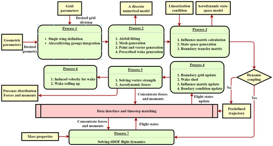
Figure 8.
Time-stepping flow chart and data structure.
3.5. Parallel Optimization
For the simulation of large-scale numerical problems, parallel optimization can greatly reduce the computational time [41]. The main idea is to make full use of the multi-core and multi-threading of the computer to carry out multiple operations that do not need data exchange and are not affected by the processing sequence. Although the UVLM is much more computationally efficient than high-order CFD, it is still time-consuming in some cases that involve models with a huge number of wakes. After analyzing the execution process and data structure of the calculation method, it was found that many calculation steps, such as wake generation, influence matrix update, and force calculation, can be constructed in the form of parallel computation. For example, the update of the influence matrix at each step requires calling the function up to times. As shown in Figure 9, the calculation of can be divided into sub-processes, each of which is allocated to a different thread. To verify the improvement of the computational efficiency achieved by parallel optimization, a time-stepping UVLM case with 256 boundary elements, 2080 wake elements, and 80 substeps was calculated on a laptop with an Intel(R) Core(TM)i7-11800H processor. The total running time and the running time of several time-consuming processes are given in Table 1. The running time of each process was reduced significantly. As the number of wake vortices is much larger than the number of boundary vortices, the efficiency improvement in the calculation of wake vortices was the most obvious. The significant improvement of the computational speed made it possible to run simulations of lager-scale models on an ordinary personal computer.
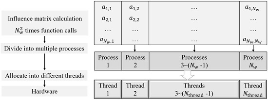
Figure 9.
Parallel optimization of influence matrix calculation.

Table 1.
Comparison of running time before and after parallel optimization.
4. Examples
4.1. Benchmark
In this section, the proposed numerical algorithm is applied for verification. It is known that the Theodorsen method is often used in the unsteady case for two-dimensional (2D) benchmark aerodynamic problems [42]. A three-dimensional (3D) infinite-span wing (with a considerable aspect ratio) is generally considered to have the same aerodynamic results as 2D models. A 3D wing with an aspect ratio of 500 was modeled to verify the proposed algorithm. The angle of attack was given as , and the reduced frequency was defined as . The unsteady pitching oscillations at different reduced frequencies were compared to show whether the algorithm was able to capture the unsteady effect. Figure 10 shows the comparison of the lift coefficients at different reduced frequencies using the Theodorsen method and the 3D UVLM method in the state-space form. Obviously, the results of the Theodorsen method and the UVLM method at different reduced frequencies were in good agreement.
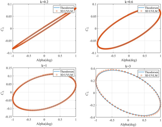
Figure 10.
Diagrams of lifting coefficient for pitch oscillations at different reduced frequencies.
In order to further validate the 3D unsteady behavior, a group of simulations of the sudden acceleration of flat rectangular wings with different aspect ratios into a constant-speed forward flight were carried out. All angles of attack were set as 5 degrees. Variations of the transient lift coefficient with time are given in Figure 11. They were in a good agreement with the results in the literature [35]. The ability of the UVLM to calculate the unsteady effect and the correctness of the program implementation were verified.
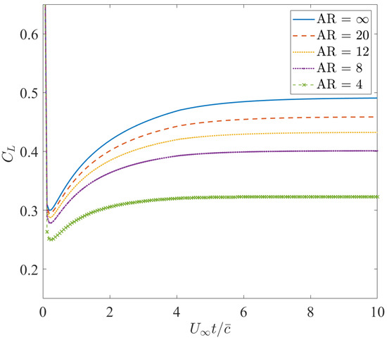
Figure 11.
Variations of the transient lift coefficient with time.
4.2. Multiple Surfaces
For the case of multiple surfaces, the Cessna 172 with a conventional fixed-wing configuration was adopted to illustrate the modeling ability of the algorithm and the aerodynamic influence between different lifting surfaces. The process of geometric modeling can be easily performed as the main wing, the vertical tail, and the horizontal tail were simplified as lifting surfaces, which were defined by fixed-format parameters and initialized as wing-type objects. In order to run the developed code, the input data of the main wing are given in Table 2 as an example. Other lifting surfaces can be defined by modifying the value of each variable in the table. The whole model was defined by three wing components with 15 sections and four airfoil types, as shown in Figure 12. The aircraft model was integrated automatically through the reference point of each lifting surface.
Table 2.
Input data of the main wing of the Cessna 172.
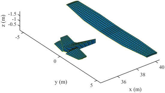
Figure 12.
Modeling of a fixed-wing aircraft with multi-lifting surfaces.
Note that the influence of aerodynamic forces between multiple lifting surfaces cannot be ignored. Intuitively, the force calculated with the consideration of the influences between multiple surfaces should be different from the one calculated independently. It is also verified in Figure 13 that the pressure distribution of the horizontal tail calculated with the consideration of the influences from other surfaces (the upper left plot) was obviously different from the one calculated independently (the bottom left plot). As shown in Table 3, the extreme values of the pressure and the total lifts were also different. Although the absolute value of total lift varied little, the effect on the pitching moment was of the same order of magnitude as the effect of the elevator. As a matter of fact, the impact of wingtip vortices on the tail control surface must be considered in the aircraft design process [43].
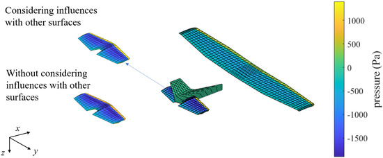
Figure 13.
Effect of other lifting surfaces on the horizontal stabilizer.
Table 3.
Comparison of aerodynamic results of the stabilizer regarding the influence from other lifting surfaces.
For some engineering applications, the influence of non-lifting surfaces must be concerned, and this can also be performed using the proposed algorithm through appropriate modeling techniques. Figure 14 gives an example of ground effect modeling, in which the ground is directly represented by a set of boundary vortices without additional derivation and code modification. The x-axis in Figure 14b is the altitude normalized by the mean aerodynamic chord length of the aircraft.
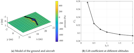
Figure 14.
Example of non-lifting surface modeling: ground effect.
4.3. Wake–Surface Interactions
The aerodynamic simulation of propeller rotation is a typical problem involving wake–boundary interactions. Figure 15a gives the distribution and strength of wake vortices around a twin blade propeller after starting for a while. The details of the geometric model and simulation parameters are given in Table 4. There are obvious overlaps between wakes and blades due to the complex induced velocity. The time history of the thrust coefficient is shown in Figure 15b. When the blades start rotating, the thrust first increases rapidly due to the strong effect of the starting vortex shedding, then it decreases with the movement of the wakes and the wake–boundary interactions and, finally, fluctuates within a relatively stable range near the experimental result given in the literature [44]. This matches how the aerodynamic force of the real propeller develops. Combined with the application in the previous section, the propeller can be modeled as a part of the whole aircraft for the aerodynamic numerical calculation of aircraft with more complex configurations.
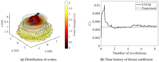
Figure 15.
Simulation results of a propeller with wake–boundary interactions.
Table 4.
Geometric parameters of the propeller model [44].
4.4. Free Flight with Rigid Body Dynamic Coupling
As described in Section 3.3, the direct coupling cannot be ignored if we need a more rigorous discussion of the impact of unsteady aerodynamics on the flight dynamics. Therefore, in this paper, the algorithm was also implemented together with the function of nonlinear flight dynamics simulation. Assume that the initial forward speed of a flying wing is 40 m/s. The resulting free glide path and time histories of the states can be obtained through the free flight simulation and are shown in Figure 16 and Figure 17, respectively. Note that the conventional aerodynamic modeling typically requires linearization around a trimmed/initial condition. Hence, the simulation was only valid around this condition, whereas the UVLM can simulate the nonlinearities without this limitation. Even if the states of the aircraft vary significantly during the simulation process, i.e., away from the initial condition, the free flight simulation can ensure the complete nonlinearity of the aerodynamic model without pre-interpolation. In addition, the open-loop simulation of complete free flight can be used for aircraft model identification, and the closed-loop simulation can be used to test the flight controllers designed based on a linearized or pre-interpolated aerodynamic model.
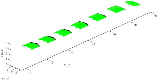
Figure 16.
The glide path of a flying wing.
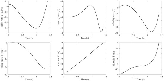
Figure 17.
Time history of kinematic states.
5. Conclusions
Based on the UVLM theory, this paper proposed an object-oriented programming approach for fast aerodynamic modeling and simulation. It can easily model objects that conform to the thin wing theory using multiple lift surfaces. The instantaneous meshing of the boundary was updated in the time step simulation. This made the modeling closer to the real physical situation and also more convenient to automatically construct the boundary conditions of various motion modes. The computation time for modeling and simulation was greatly reduced through the parallel optimization.
The unsteady effect considered in this paper was examined through pitch oscillations. Three different cases were given to demonstrate the modeling capability and the application range of the proposed approach. In the first case, the program was implemented to simulate fixed-wing aircraft with multi-lifting surfaces and the ground effect where the ground was modeled as a set of static boundary vortices. In the second case, taking a propeller as an example, the program was used to model wake–boundary interactions, and this resulted in great application potential to more complex scenarios. Lastly, as an example of the direct coupling between aerodynamics and flight dynamics calculations, the program was used to simulate the free flight of a flying wing, and the results showed that the program provides a simulation environment with the consideration of real-time unsteady aerodynamic forces.
In summary, by adopting object-oriented structures, innovative processing of the boundary conditions, and direct integration with the flight dynamics, the proposed UVLM-based aerodynamic modeling algorithm is computationally efficient and suitable for engineering applications.
Author Contributions
Conceptualization, Q.L. and W.G.; methodology, W.G. and Y.L.; software, W.G.; validation, Y.L.; resources, Q.L. and B.L.; writing—original draft preparation, W.G.; writing—review and editing, all authors; supervision, B.L.; project administration, Q.L. All authors have read and agreed to the published version of the manuscript.
Funding
This research received no external funding.
Institutional Review Board Statement
Not applicable.
Informed Consent Statement
Not applicable.
Data Availability Statement
All data used during the study appear in the submitted article.
Conflicts of Interest
The authors declare no conflict of interest.
References
- Xu, H.; Han, J.; Yun, H.; Chen, X. Calculation of the Hinge Moments of a Folding Wing Aircraft during the Flight-Folding Process. Int. J. Aerosp. Eng. 2019, 2019, 1–11. [Google Scholar] [CrossRef]
- Tian, Y.; Quan, J.; Liu, P.; Li, D.; Kong, C. Mechanism/Structure/Aerodynamic Multidisciplinary Optimization of Flexible High-lift Devices for Transport Aircraft. Aerosp. Sci. Technol. 2019, 93, 104813. [Google Scholar] [CrossRef]
- Wang, I.; Gibbs, S.C.; Dowell, E.H. Aeroelastic Model of Multisegmented Folding Wings: Theory and Experiment. J. Aircr. 2012, 49, 911–921. [Google Scholar] [CrossRef]
- Panagiotou, P.; Dimopoulos, T.; Dimitriou, S.; Yakinthos, K. Quasi-3D Aerodynamic Analysis Method for Blended-Wing-Body UAV Configurations. Aerospace 2020, 8, 13. [Google Scholar] [CrossRef]
- Cole, J.A.; Maughmer, M.D.; Bramesfeld, G.; Melville, M.; Kinzel, M. Unsteady Lift Prediction with a Higher-Order Potential Flow Method. Aerospace 2020, 7, 60. [Google Scholar] [CrossRef]
- Shahid, T.; Sajjad, F.; Ahsan, M.; Farhan, S.; Salamat, S.; Abbas, M. Comparison of Flow-Solvers: Linear Vortex Lattice Method and Higher-Order Panel Method with Analytical and Wind Tunnel Data. In Proceedings of the 2020 3rd International Conference on Computing, Mathematics and Engineering Technologies (iCoMET), Sukkur, Pakistan, 29–30 January 2020; pp. 1–7. [Google Scholar] [CrossRef]
- Kontogiannis, A.; Laurendeau, E. Adjoint State of Nonlinear Vortex-Lattice Method for Aerodynamic Design and Contro. AIAA J. 2021, 59, 1184–1195. [Google Scholar] [CrossRef]
- Go, Y.J.; Bae, J.H.; Ryi, J.; Choi, J.S.; Lee, C.R. A Study on the Scale Effect According to the Reynolds Number in Propeller Flow Analysis and a Model Experiment. Aerospace 2022, 9, 559. [Google Scholar] [CrossRef]
- Albano, E.; Rodden, W.P. A Doublet-Lattice Method for Calculating Lift Distributions on Oscillating Surfaces in Subsonic Flows. AIAA J. 1969, 7, 279–285. [Google Scholar] [CrossRef]
- Kidane, B.S.; Troiani, E. Static Aeroelastic Beam Model Development for Folding Winglet Design. Aerospace 2022, 7, 106. [Google Scholar] [CrossRef]
- Kier, T. Comparison of Unsteady Aerodynamic Modelling Methodologies with Respect to Flight Loads Analysis. In Proceedings of the AIAA Atmospheric Flight Mechanics Conference and Exhibit, San Francisco, CA, USA, 15–18 August 2005. [Google Scholar] [CrossRef]
- Konstadinopoulos, P.; Thrasher, D.F.; Mook, D.T.; Nayfeh, A.H.; Watson, L. A Vortex-Lattice Method for General, Unsteady Aerodynamics. J. Aircr. 1985, 22, 43–49. [Google Scholar] [CrossRef]
- Belotserkovskii, S.M. Study of the Unsteady Aerodynamics of Lifting Surfaces Using the Computer. Annu. Rev. Fluid Mech. 2003, 9, 469–494. [Google Scholar] [CrossRef]
- Gordillo, A.M.P.; Santos, J.S.V.; Mejia, O.D.L.; Collazos, L.J.S.; Escobar, J.A. Numerical and Experimental Estimation of the Efficiency of a Quadcopter Rotor Operating at Hover. Energies 2019, 12, 261. [Google Scholar] [CrossRef]
- Proulx-Cabana, V.; Nguyen, M.T.; Prothin, S.; Michon, G.; Laurendeau, E. A Hybrid Non-Linear Unsteady Vortex Lattice-Vortex Particle Method for Rotor Blades Aerodynamic Simulations. Fluids 2022, 7, 81. [Google Scholar] [CrossRef]
- Hall, B.D.; Mook, D.T.; Nayfeh, A.H.; Preidikman, S. Novel Strategy for Suppressing the Flutter Oscillations of Aircraft Wings. AIAA J. 2001, 39, 1843–1850. [Google Scholar] [CrossRef]
- Maraniello, S.; Palacios, R. Parametric Reduced-Order Modeling of the Unsteady Vortex-Lattice Method. AIAA J. 2020, 58, 1–15. [Google Scholar] [CrossRef]
- Wang, Z.; Chen, P.C.; Liu, D.D.; Mook, D.T.; Patil, M.J. Time Domain Nonlinear Aeroelastic Analysis for HALE Wings. In Proceedings of the 47th AIAA/ASME/ASCE/AHS/ASC Structures, Structural Dynamics, and Materials Conference, Newport, RI, USA, 1–4 May 2006. [Google Scholar] [CrossRef]
- Stanford, B.; Beran, P. Formulation of Analytical Design Derivatives for Nonlinear Unsteady Aeroelasticity. AIAA J. 2011, 49, 598–610. [Google Scholar] [CrossRef]
- Obradovic, B.; Subbarao, K. Modeling of Flight Dynamics of Morphing Wing Aircraft. J. Aircr. 2012, 48, 391–402. [Google Scholar] [CrossRef]
- Jung, Y.Y.; Kim, J.H. Unsteady Subsonic Aerodynamic Characteristics of Wing in Fold Motion. Int. J. Aeronaut. Space Sci. 2011, 12, 63–68. [Google Scholar] [CrossRef]
- Stewart, E.C.; Patil, M.J.; Canfield, R.A.; Snyder, R.D. Aeroelastic Shape Optimization of a Flapping Wing. J. Aircr. 2016, 53, 636–650. [Google Scholar] [CrossRef]
- Murua, J.; Palacios, R.; Graham, J.M.R. Applications of the Unsteady Vortex-Lattice Method in Aircraft Aeroelasticity and Flight Dynamics. Prog. Aerosp. Sci. 2012, 55, 46–72. [Google Scholar] [CrossRef]
- Binder, S.; Wildschek, A.; Breuker, R.D. Aeroelastic Stability Analysis of the FLEXOP Demonstrator using the Continuous Time Unsteady Vortex Lattice Method. In Proceedings of the 2018 AIAA/ASCE/AHS/ASC Structures, Structural Dynamics, and Materials Conference, Kissimmee, FL, USA, 8–12 January 2018. [Google Scholar] [CrossRef]
- Jeon, M.; Lee, S.; Kim, T.; Lee, S. Wake Influence on Dynamic Load Characteristics of Offshore Floating Wind Turbines. AIAA J. 2016, 54, 1–11. [Google Scholar] [CrossRef]
- Kim, H.; Lee, S.; Son, E.; Lee, S.; Lee, S. Aerodynamic Noise Analysis of Large Horizontal Axis Wind Turbines Considering Fluid-Structure Interaction. Renew. Energy 2012, 42, 46–53. [Google Scholar] [CrossRef]
- Nguyen, A.T.; Kim, J.K.; Han, J.S.; Han, J.H. Extended Unsteady Vortex-Lattice Method for Insect Flapping Wings. J. Aircr. 2016, 53, 1709–1718. [Google Scholar] [CrossRef]
- Lee, S.G.; Yang, H.H.; Addo-Akoto, R.; Han, J.H. Transition Flight Trajectory Optimization for a Flapping-Wing Micro Air Vehicle with Unsteady Vortex-Lattice Method. Aerospace 2022, 9, 660. [Google Scholar] [CrossRef]
- Thomas, D.; Cerquaglia, M.L.; Boman, R.; Economon, T.D.; Alonso, J.J.; Dimitriadis, G.; Terrapon, V.E. CUPyDO—An Integrated Python Environment for Coupled Fluid-Structure Simulations. Adv. Eng. Softw. 2019, 128, 69–85. [Google Scholar] [CrossRef]
- Budziak, K. Aerodynamic Analysis with Athena Vortex Lattice (AVL); Aircraft Design and Systems Group (AERO), Department of Automotive and Aeronautical Engineering: Hamburg, Germany, 2015. [Google Scholar] [CrossRef]
- Melin, T. User’s Guide and Reference Manual for Tornado; Royal Institute of Technology (KTH), Department of Aeronautics: Stockholm, Sweden, 2000. [Google Scholar]
- Melin, T. A Vortex Lattice MATLAB Implementation for Linear Aerodynamic Wing Applications. Master’s Thesis, Royal Institute of Technology (KTH), Department of Aeronautics, Stockholm, Sweden, 2000. [Google Scholar]
- Communier, D.; Salinas, M.F.; Moyao, O.C.; Botez, R.M. Aero Structural Modeling of a Wing Using CATIA V5 and XFLR5 Software and Experimental Validation Using the Price- Païdoussis Wing Tunnel. In Proceedings of the AIAA Aviation, AIAA Atmospheric Flight Mechanics Conference, Dallas, TX, USA, 22–26 June 2015. [Google Scholar] [CrossRef]
- del Carre, A.; Muñoz-Simón, A.; Goizueta, N.; Palacios, R. SHARPy: A Dynamic Aeroelastic Simulation Toolbox for Very Flexible Aircraft and Wind Turbines. J. Open Source Softw. 2019, 4, 1885. [Google Scholar] [CrossRef]
- Katz, J.; Plotkin, A. Low-Speed Aerodynamics; Cambridge University Press: Cambridge, UK, 2001. [Google Scholar]
- Ford, C.W.P.; Babinsky, H. Lift and the Leading-Edge Vortex. J. Fluid Mech. 2013, 720, 280–313. [Google Scholar] [CrossRef]
- Vatistas, G.H.; Panagiotakakos, G.D.; Manikis, F.I. Extension of the n-Vortex Model to Approximate the Effects of Turbulence. J. Aircr. 2015, 52, 1721–1725. [Google Scholar] [CrossRef]
- Simpson, R.J.S.; Palacios, R.; Murua, J. Induced-drag Calculations in the Unsteady Vortex Lattice Method. AIAA J. 2013, 51, 1775–1779. [Google Scholar] [CrossRef]
- Mohammadi-Amin, M.; Ghadiri, B.; Abdalla, M.M.; Haddadpour, H.; Breuker, R.D. Continuous-Time State-Space Unsteady Aerodynamic Modeling Based on Boundary Element Method. Eng. Anal. Bound. Elem. 2012, 36, 789–798. [Google Scholar] [CrossRef]
- Beard, R.W.; Mclain, T.W. Small Unmanned Aircraft: Theroy and Practice; Princeton University Press: Princeton, NJ, USA, 2012. [Google Scholar]
- Rauber, T.; Rünger, G. Parallel Programming; Springer: Berlin/Heildeberg, German, 2013. [Google Scholar] [CrossRef]
- Fernandez-Escudero, C.; Gagnon, M.; Laurendeau, E.; Prothin, S.; Michon, G.; Ross, A. Comparison of Low, Medium and High Fidelity Numerical Methods for Unsteady Aerodynamics and Nonlinear Aeroelasticity. J. Fluids Struct. 2019, 91, 102744. [Google Scholar] [CrossRef]
- Hoang, N.T.B.; Bui, B.V. Experimental and Numerical Studies of Wingtip and Downwash Effects on Horizontal Tail. J. Mech. Sci. Technol. 2019, 33, 649–659. [Google Scholar] [CrossRef]
- Caradonna, F.X.; Tung, C. Experimental and Analytical Studies of a Model Helicopter Rotor in Hover. In Proceedings of the European Rotorcraft and Powered Lift Aircraft Forum, Bristol, UK, 1 September 1981. [Google Scholar]


Disclaimer/Publisher’s Note: The statements, opinions and data contained in all publications are solely those of the individual author(s) and contributor(s) and not of MDPI and/or the editor(s). MDPI and/or the editor(s) disclaim responsibility for any injury to people or property resulting from any ideas, methods, instructions or products referred to in the content. |
© 2023 by the authors. Licensee MDPI, Basel, Switzerland. This article is an open access article distributed under the terms and conditions of the Creative Commons Attribution (CC BY) license (https://creativecommons.org/licenses/by/4.0/).