
Bayesian Optimization for Fine-Tuning EKF Parameters in UAV Attitude and Heading Reference System Estimation


Abstract
:1. Introduction
2. Mathematical Formulations
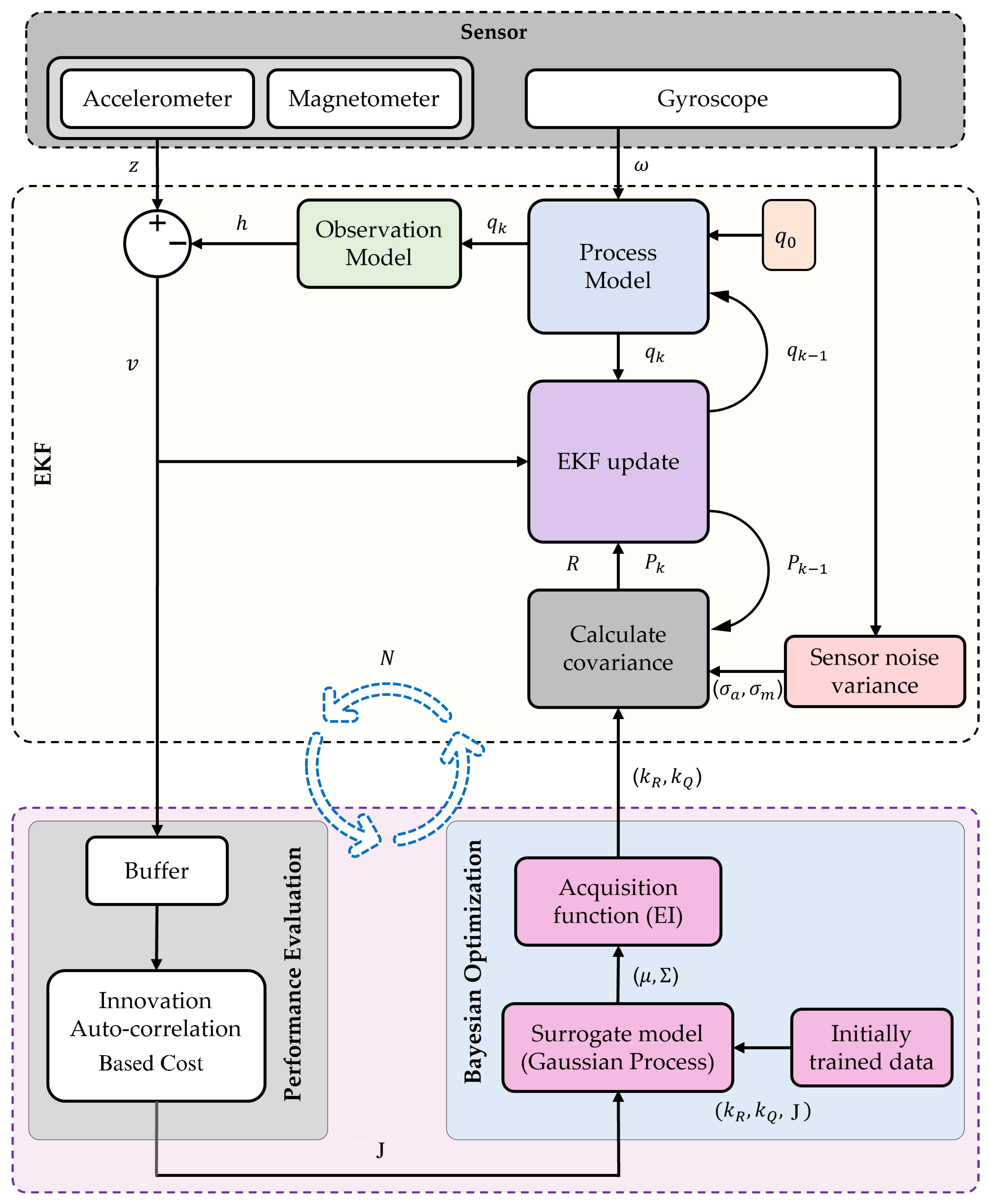
2.1. Extended Kalman Filter (EKF) Equations
2.1.1. Attitude Propagation Model
Process Noise Covariance Calculation
2.1.2. Attitude and Heading Observation Modeling
Measurement Noise Covariance Calculation
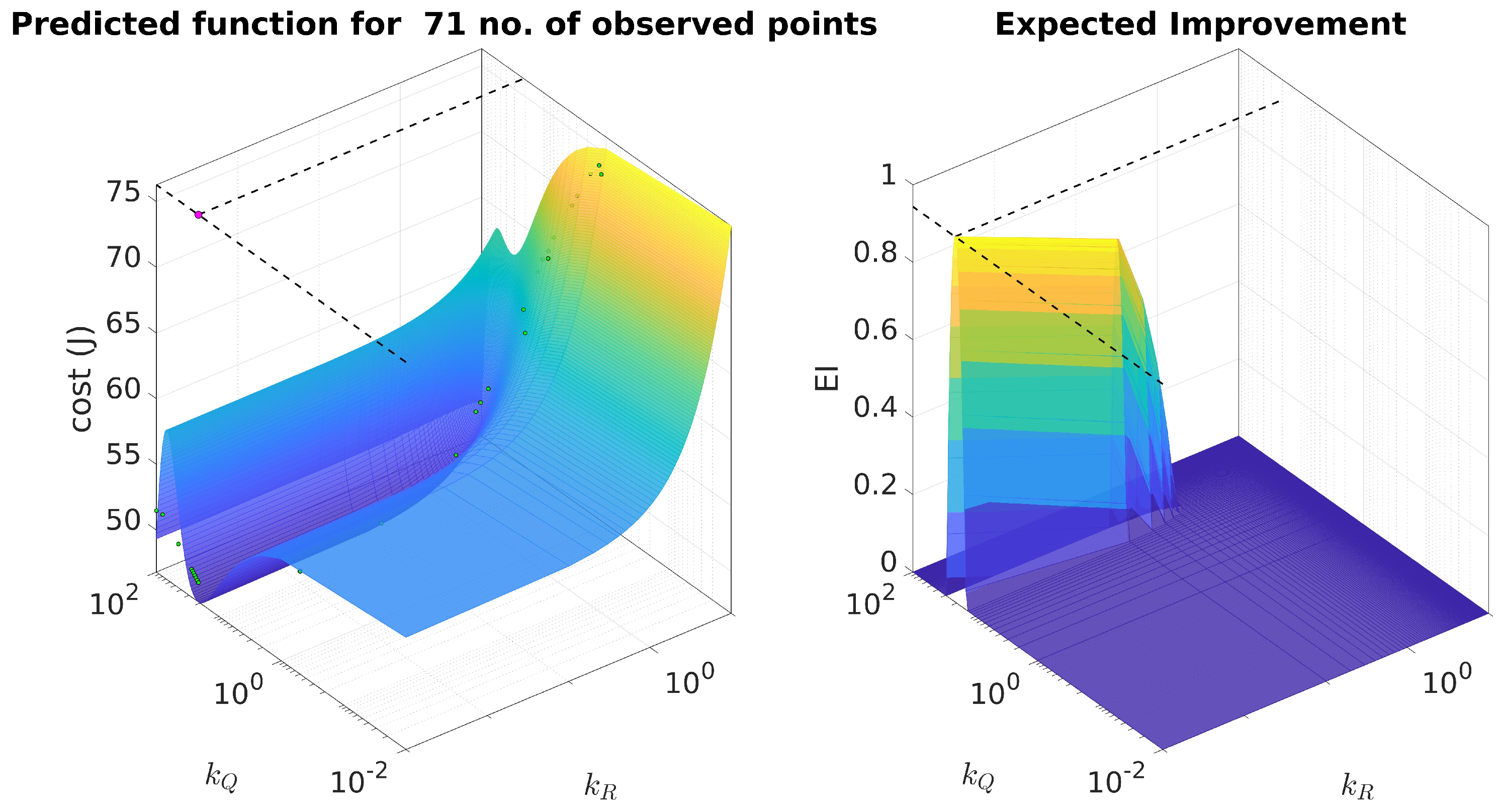
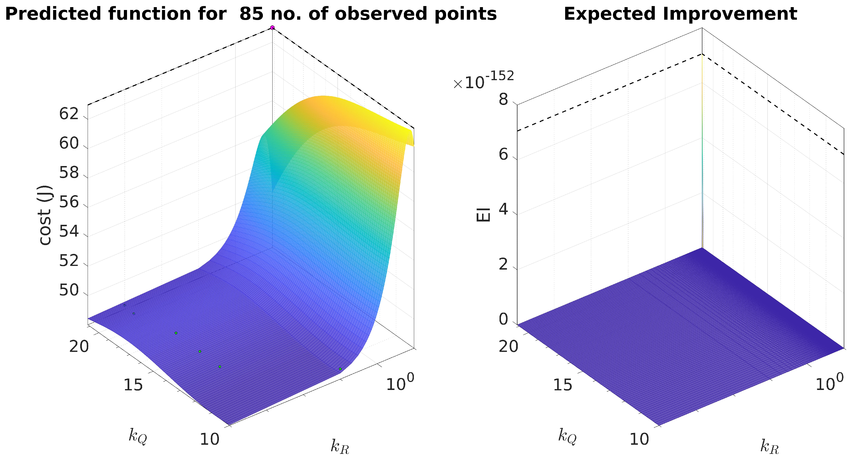
2.2. Bayesian Optimization
2.2.1. Gaussian Process (GP) Regression
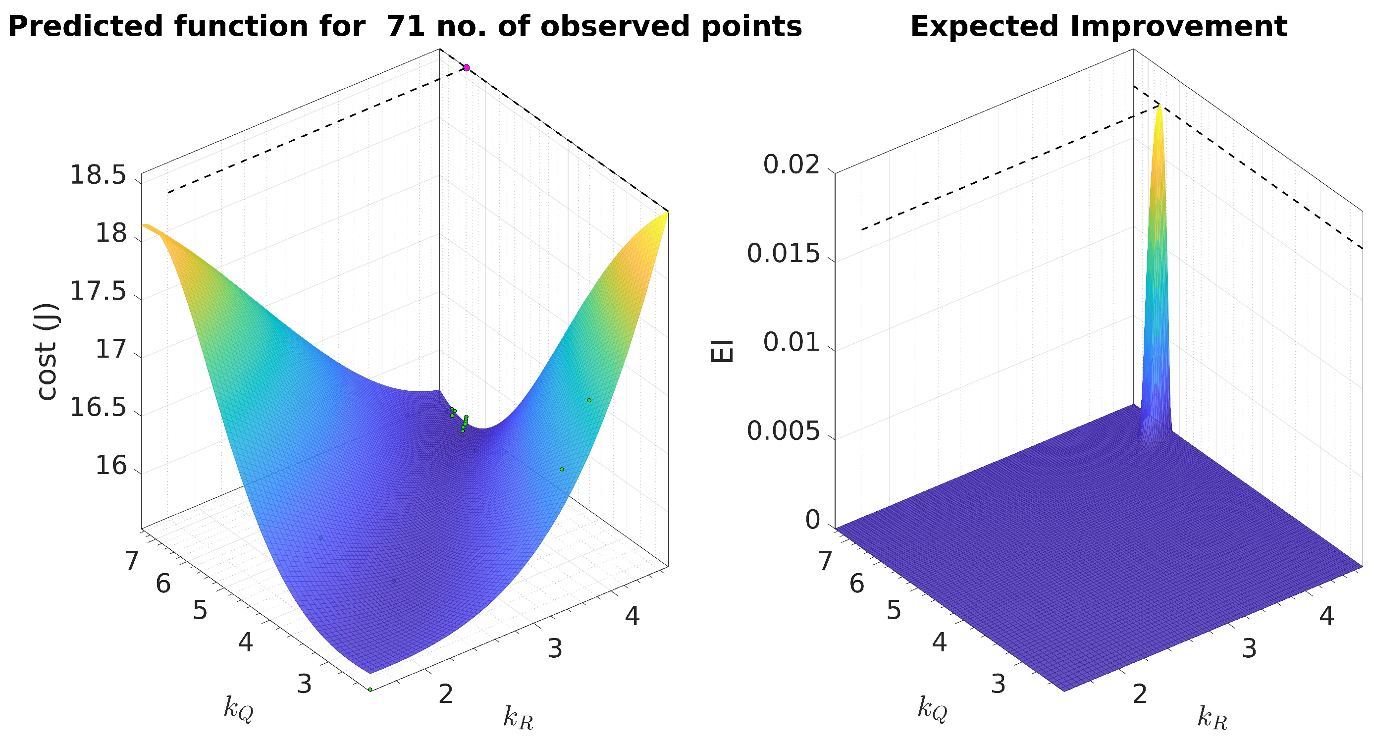
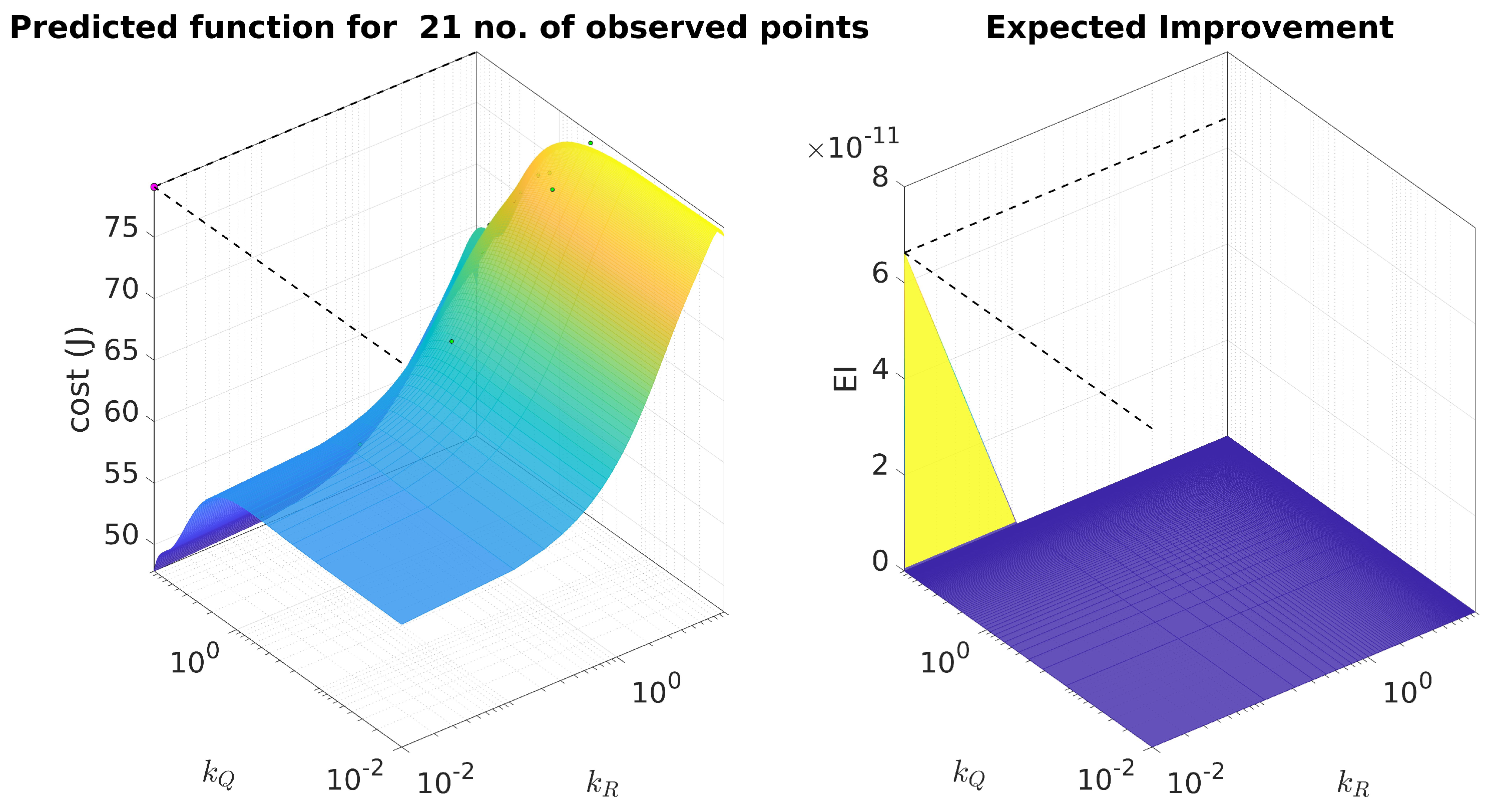
2.2.2. Acquisition Function
3. Process and Measurement Noise Covariance Tuning with Bayesian Optimization
3.1. Adaptive Search Region for Bayesian Optimization
3.2. Optimization Cost Function
4. Testing
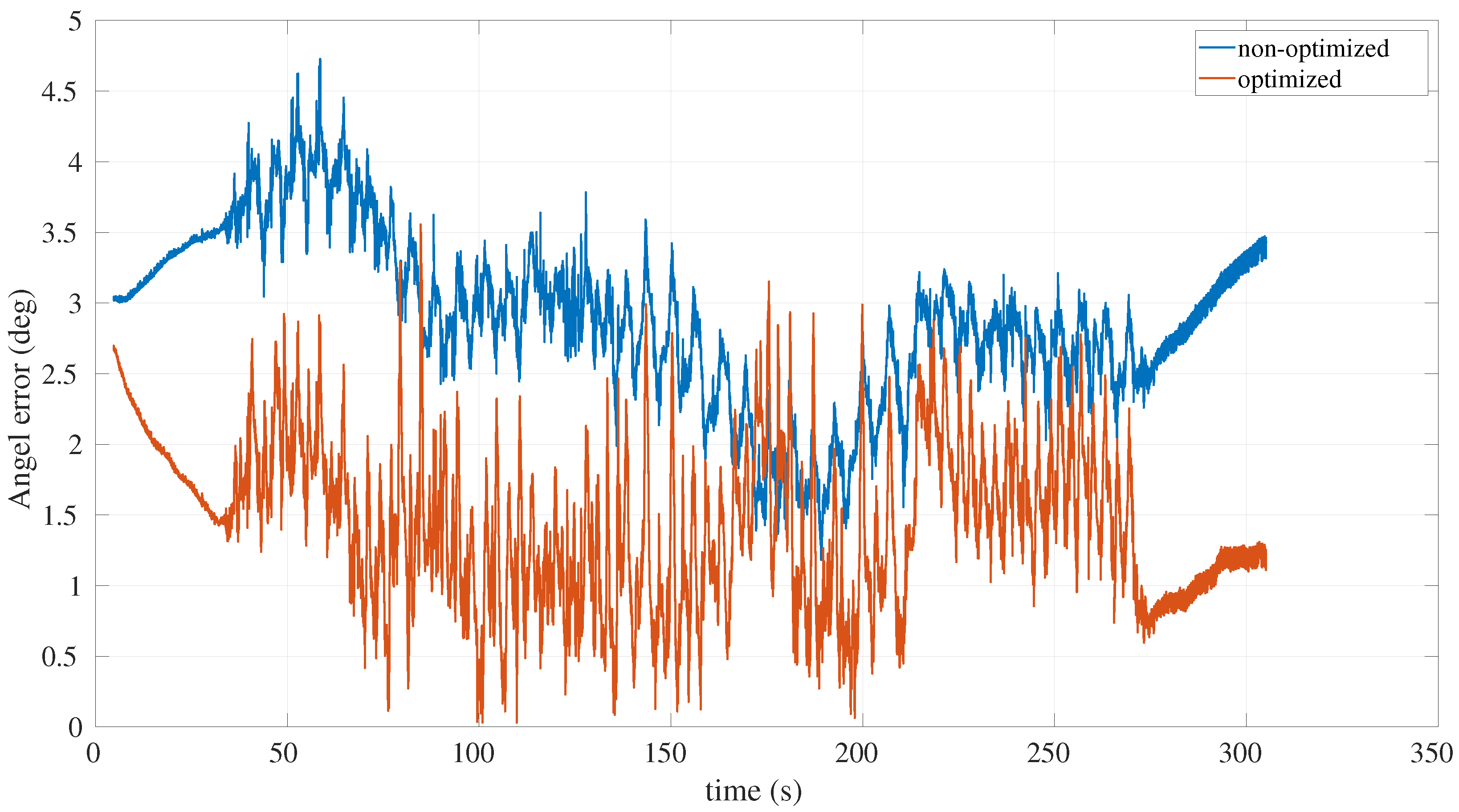
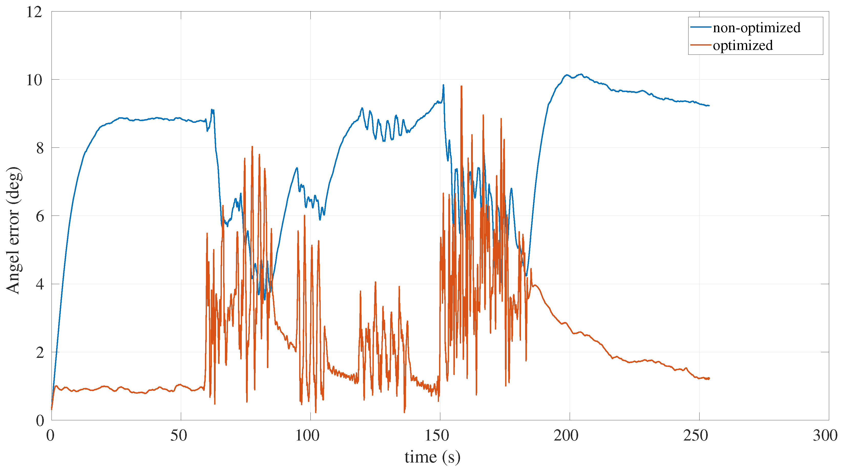
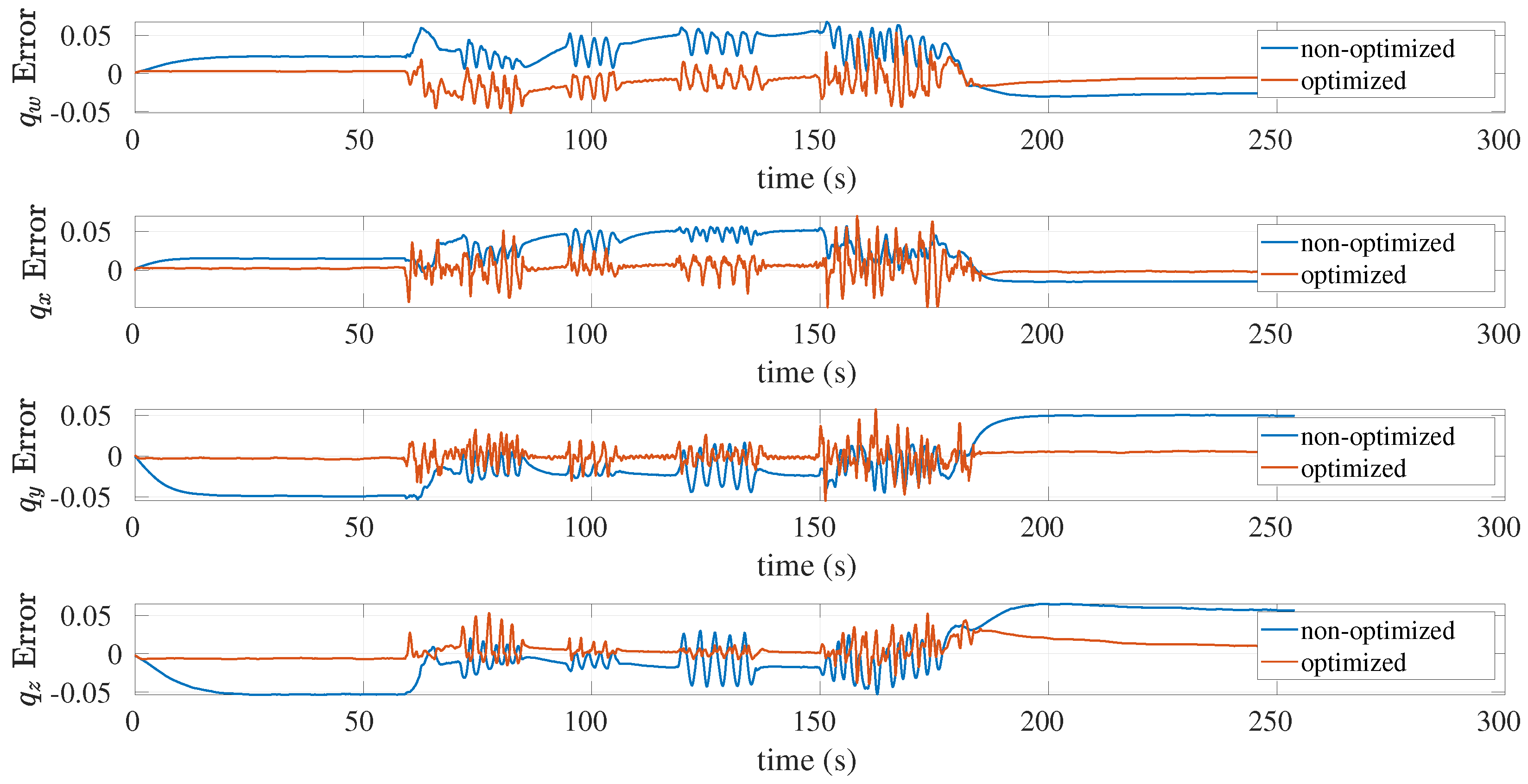
4.1. Test Results
4.1.1. Case BOARD Dataset:
4.1.2. Case SASARI Dataset:
5. Discussion
6. Conclusions
Author Contributions
Funding
Data Availability Statement
Conflicts of Interest
Abbreviations
| KF | Kalman Filter |
| EKF | extended Kalman filter |
| UAV | unmanned aerial vehicle |
| AHRS | attitude and heading reference system |
| 3D | 3-dimension |
| CM | covariance matrix |
| ANN | artificial neural network |
| RPE | recursive prediction error |
| NED | north east down |
| GP | Gaussian process |
| EI | expected improvement |
| probability density function | |
| CDF | cumulative distribution function |
| IMU | inertial measurement unit |
| NIS | normalized innovation squared |
| RMS | root mean square |
References
- Saha, M.; Goswami, B.; Ghosh, R. Two novel costs for determining the tuning parameters of the Kalman Filter. arXiv 2011, arXiv:1110.3895. [Google Scholar] [CrossRef]
- Pieter, A.; Adam, C.; Michael, M.; Andrew, N.; Sebastian, T. Discriminative Training of Kalman Filters. Robot. Sci. Syst. 2005, 52, 1401–1406. [Google Scholar]
- Carew, B.; Belanger, P. Identification of optimum filter steady-state gain for systems with unknown noise covariances. IEEE Trans. Autom. Control 1973, 18, 582–587. [Google Scholar] [CrossRef]
- Mehra, R. Approaches to adaptive filtering. IEEE Trans. Autom. Control 1972, 17, 693–698. [Google Scholar] [CrossRef]
- Duník, J.; Straka, O.; Kost, O.; Havlík, J. Noise covariance matrices in state-space models: A survey and comparison of estimation methods—Part I. Int. J. Adapt. Control. Signal Process. 2017, 31, 1505–1543. [Google Scholar] [CrossRef]
- Gelen, A.G.; Atasoy, A. A New Method for Kalman Filter Tuning. In Proceedings of the 2018 International Conference on Artificial Intelligence and Data Processing (IDAP), Malatya, Turkey, 28–30 September 2018. [Google Scholar] [CrossRef]
- Åkesson, B.M.; Jørgensen, J.B.; Poulsen, N.K.; Jørgensen, S.B. A tool for Kalman filter tuning. Comput. Aided Chem. Eng. 2007, 24, 859–864. [Google Scholar] [CrossRef]
- Odelson, B.J.; Rajamani, M.R.; Rawlings, J.B. A new autocovariance least-squares method for estimating noise covariances. Automatica 2006, 42, 303–308. [Google Scholar] [CrossRef]
- Jindrich, D.; Oliver, K.; Ondřej, S. Design of measurement difference autocovariance method for estimation of process and measurement noise covariances. Automatica 2018, 90, 16–24. [Google Scholar] [CrossRef]
- Mehra, R. On the identification of variances and adaptive Kalman filtering. IEEE Trans. Autom. Control 1970, 15, 175–184. [Google Scholar] [CrossRef]
- Zhang, A.; Atia, M.M. An efficient tuning framework for Kalman filter parameter optimization using design of experiments and genetic algorithms. J. Inst. Navig. 2020, 67, 775–793. [Google Scholar] [CrossRef]
- Chhabra, A.; Venepally, J.R.; Kim, D. Measurement Noise Covariance-Adapting Kalman Filters for Varying Sensor Noise Situations. Sensors 2021, 21, 8304. [Google Scholar] [CrossRef]
- Yuen, K.-V.; Liang, P.-F.; Kuok, S.-C. Online estimation of noise parameters for Kalman filter. Struct. Eng. Mech. 2013, 47, 361–381. [Google Scholar] [CrossRef]
- Riva, M.H.; Beckmann, D.; Dagen, M.; Ortmaier, T. Online Parameter and Process Covariance Estimation using adaptive EKF and SRCuKF approaches. In Proceedings of the 2015 IEEE Conference on Control Applications (CCA), Sydney, Australia, 21 September 2015. [Google Scholar] [CrossRef]
- Ullah, I.; Fayaz, M.; Kim, D. Improving Accuracy of the Kalman Filter Algorithm in Dynamic Conditions Using ANN-Based Learning Module. Symmetry 2019, 11, 94. [Google Scholar] [CrossRef]
- Ayyarao, S.T.; Ramanarao, P. Tuning of extended Kalman filter for power systems using two lbest particle swarm optimization. IJCTA 2017, 10, 197–206. [Google Scholar]
- Chen, Z.; Heckman, C.; Julier, S.; Ahmed, N. Weak in the NEES?: Auto-tuning Kalman Filters with Bayesian Optimization. arXiv 2018, arXiv:1807.08855. [Google Scholar] [CrossRef]
- Chen, Z.; Ahmed, N.; Julier, S.; Heckman, C. Kalman Filter Tuning with Bayesian Optimization. arXiv 2019, arXiv:1912.08601. [Google Scholar] [CrossRef]
- Park, S.; Gil, M.-S.; Im, H.; Moon, Y.-S. Measurement Noise Recommendation for Efficient Kalman Filtering over a Large Amount of Sensor Data. Sensors 2019, 19, 1168. [Google Scholar] [CrossRef] [PubMed]
- Wondosen, A.; Jeong, J.-S.; Kim, S.-K.; Debele, Y.; Kang, B.-S. Improved Attitude and Heading Accuracy with Double Quaternion Parameters Estimation and Magnetic Disturbance Rejection. Sensors 2021, 21, 5475. [Google Scholar] [CrossRef]
- Sabatini, A.M. Kalman-Filter-Based Orientation Determination Using Inertial/Magnetic Sensors: Observability Analysis and Performance Evaluation. Sensors 2011, 11, 9182. [Google Scholar] [CrossRef]
- Valenti, R.G.; Dryanovski, I.; Xiao, J. A Linear Kalman Filter for MARG Orientation Estimation Using the Algebraic Quaternion Algorithm. IEEE Trans. Instrum. Meas. 2016, 65, 467–481. [Google Scholar] [CrossRef]
- Guo, S.; Wu, J.; Wang, Z.; Qian, J. Novel MARG-Sensor Orientation Estimation Algorithm Using Fast Kalman Filter. J. Sens. 2017, 2017, 8542153. [Google Scholar] [CrossRef]
- René, S.; Christos, G. How To NOT Make the Extended Kalman Filter Fail. Ind. Eng. Chem. Res. 2013, 52, 3354–3362. [Google Scholar] [CrossRef]
- Laidig, D.; Caruso, M.; Cereatti, A.; Seel, T. BROAD—A Benchmark for Robust Inertial Orientation Estimation. Data 2021, 6, 72. [Google Scholar] [CrossRef]
- Caruso, M.; Sabatini, A.M.; Laidig, D.; Seel, T.; Knaflitz, M.; Della Croce, U.; Cereatti, A. Analysis of the Accuracy of Ten Algorithms for Orientation Estimation Using Inertial and Magnetic Sensing under Optimal Conditions: One Size Does Not Fit All. Sensors 2021, 21, 2543. [Google Scholar] [CrossRef]


| Sensors Specs | Datasets | |
|---|---|---|
| BOARD [25] | SASARI [26] | |
| Accel noise () | ||
| Gyro noise () | ||
| Mag noise () | ||
| Model | myon aktos-t | Xsens-MTx |
| Datasets | Quaternion Estimation Error (RMS) | Angle Axis Representation | |||||
|---|---|---|---|---|---|---|---|
| Angle Error (RMS) | |||||||
| BOARD | 1 | 1 | 0.0140 | 0.0115 | 0.0110 | 0.0147 | 2.8941 |
| 1.22 | 7.3 | 0.0074 | 0.0067 | 0.0047 | 0.0087 | 1.4832 | |
| Improvement | 47.14 % | 41.74% | 57.27% | 40.82% | 48.75% | ||
| SASARI | 1 | 1 | 0.0326 | 0.0287 | 0.0372 | 0.0413 | 7.8811 |
| 0.1 | 10.0 | 0.0138 | 0.0113 | 0.0091 | 0.0129 | 2.2604 | |
| Improvement | 57.67% | 60.63% | 75.54% | 68.77% | 71.32% | ||
Disclaimer/Publisher’s Note: The statements, opinions and data contained in all publications are solely those of the individual author(s) and contributor(s) and not of MDPI and/or the editor(s). MDPI and/or the editor(s) disclaim responsibility for any injury to people or property resulting from any ideas, methods, instructions or products referred to in the content. |
© 2023 by the authors. Licensee MDPI, Basel, Switzerland. This article is an open access article distributed under the terms and conditions of the Creative Commons Attribution (CC BY) license (https://creativecommons.org/licenses/by/4.0/).
Share and Cite
Wondosen, A.; Debele, Y.; Kim, S.-K.; Shi, H.-Y.; Endale, B.; Kang, B.-S. Bayesian Optimization for Fine-Tuning EKF Parameters in UAV Attitude and Heading Reference System Estimation. Aerospace 2023, 10, 1023. https://doi.org/10.3390/aerospace10121023
Wondosen A, Debele Y, Kim S-K, Shi H-Y, Endale B, Kang B-S. Bayesian Optimization for Fine-Tuning EKF Parameters in UAV Attitude and Heading Reference System Estimation. Aerospace. 2023; 10(12):1023. https://doi.org/10.3390/aerospace10121023
Chicago/Turabian StyleWondosen, Assefinew, Yisak Debele, Seung-Ki Kim, Ha-Young Shi, Bedada Endale, and Beom-Soo Kang. 2023. "Bayesian Optimization for Fine-Tuning EKF Parameters in UAV Attitude and Heading Reference System Estimation" Aerospace 10, no. 12: 1023. https://doi.org/10.3390/aerospace10121023
APA StyleWondosen, A., Debele, Y., Kim, S.-K., Shi, H.-Y., Endale, B., & Kang, B.-S. (2023). Bayesian Optimization for Fine-Tuning EKF Parameters in UAV Attitude and Heading Reference System Estimation. Aerospace, 10(12), 1023. https://doi.org/10.3390/aerospace10121023