1. Introduction
Many space missions prefer to utilize low-thrust propulsion systems because they have higher specific impulse compared with high-thrust propulsion systems that significantly decreases the quantity of the propellant used. Two commonly used approaches to low-thrust optimal control problems are indirect and direct methods [
1,
2]. Indirect methods utilize the Pontryagin maximum principle, which transforms the optimal control problem into a two-point boundary value problem [
3,
4,
5]. Using indirect optimization, the global search for fuel-optimal low-thrust transfers from a low Earth orbit to the vicinity of the Moon was performed in the Earth–Moon planar circular restricted three-body problem [
6]. Extensive research and classification of low-thrust low-energy transfers between low Earth and lunar orbits using indirect optimal control are thoroughly examined in [
7]. On the other hand, direct methods rely on discretization/parametrization and transform the optimal control problem into a nonlinear programming problem [
8,
9,
10] to solve transfer [
11], rephasing [
12], and rendezvous [
13,
14,
15,
16] problems. Both approaches struggle with significant sensitivity to the initial guess, lead to numerous local extrema, and incur high computational costs during the optimization process. To overcome these difficulties, various methods are used [
17], including modified continuation techniques [
18], search space landscape analysis [
19], convexification [
20,
21], and neural control [
22,
23].
Both direct and indirect methods often use averaging as a key preliminary step in solving low-thrust optimization problems. The averaged equations provide an overview of the orbit’s mean evolution, excluding short-term oscillations resulting from the thrust or disturbances. Additionally, they are numerically more stable than the system without averaging. The application of averaging allows for a fast and accurate search for optimal orbital transfers [
24,
25,
26]. In [
27,
28], analytical solutions of minimum fuel and minimum energy transfer problems were achieved for close elliptic coplanar orbits using the Pontryagin principle with the averaging of the Hamiltonian.
Averaging is also applied within the direct optimization framework. According to a study [
29], when the thrust (or perturbation) is a function with a constant spectrum, the averaged right-hand side of the Gauss variational equations depends solely on 14 thrust-perturbation Fourier coefficients. This fact was used to define low-thrust control using a finite number of variables and solve an optimal control problem using direct methods [
30]. However, the classical orbital elements used in [
29] are singular in the instances of circular and equatorial orbits. Additionally, the averaged variational equations in classical orbital elements are not integrable.
The authors present an advancement of the above approach in the current study. By expressing the spacecraft orbital motion in terms of modified equinoctial elements and taking the eccentric longitude as a fast variable, we found that the averaged equations of motion contain only 13 Fourier coefficients. Moreover, a closed-form solution for cases with low eccentricity is found. Now we are interested in the application of this averaging technique with analytical formulas to multiorbit low-thrust transfer optimization problems. The essence of this work is the reduction of the optimal control problem to a nonlinear programming problem with a small number of optimization parameters and its solution.
This paper is organized as follows.
Section 2 presents the general optimal control problem that is under investigation.
Section 3.1 explains the developed averaging approach. Then, in
Section 3.2, the case of transfer between near-circular orbits is formalized, and the corresponding closed-form solution of the averaged equations is presented.
Section 4 outlines the process of transforming the optimal control problem into nonlinear programming using the averaging method. In
Section 5, two test energy-optimal control problems are defined and solved: orbital transfer near the geostationary orbit (
Section 5.1) and circular orbit raising maneuver (
Section 5.2).
Section 5.3 compares the optimal solutions with the Pontryagin extremals, which were obtained using the Pontryagin maximum principle. The final section draws conclusions from the study and suggests directions for further research on the topic.
2. The General Optimal Control Problem under Study
The perturbed orbital motion of the spacecraft in the vicinity of the center of attraction is considered. The motion of the spacecraft is described by a system of differential equations in terms of the modified equinoctial elements as follows [
31]:
where
Here,
p,
,
,
, and
are the modified equinoctial elements that are related to the semimajor axis
a, eccentricity
e, inclination
i, right ascension of the ascending node
, and argument of periapsis
by the expressions [
31]
The variable F is the eccentric longitude; it relates to , , and the eccentric anomaly E by the expression . The perturbation variables , , and are the projections of the perturbation acceleration on the axes of the local-vertical/local-horizontal frame; is the radial component; is the component orthogonal to the radius vector of the spacecraft; and is the component normal to the orbital plane. The parameter is the gravitational parameter of the attracting body.
The equations above can be written in a compact form:
where
is a vector of modified equinoctial elements, and
and
are the right-hand side of Equations (
1)–(
6).
In the current study, the optimal control problem between two points of phase space characterized by the elements and the eccentric longitudes
and
in a given time interval
governed by Equations (
8) is considered. In the current work, no other perturbations other than thrust are considered. The objective for minimization is
This is the general minimum-energy transfer optimal control problem between two phase states in a given time [
1]. It can be easily shown that in the case of an ideally regulated engine, this problem is equivalent to minimizing the fuel costs for a transfer between the two points in a given time.
Let us now proceed to the description of the averaging method used in this work.
3. The Averaging Technique and Approximate Solutions
3.1. Averaged Variational Equations in Modified Equinoctial Elements
In this section, we briefly describe the technique of obtaining the averaged variational equations and present the result of averaging. For that purpose, we first represent the perturbation acceleration by the Fourier series:
where
and
are the Fourier series coefficients, and the upper script indicates one of the acceleration components. This representation allows us to average the right-hand sides of the variational equations on
p,
,
,
, and
over the mean longitude
over one revolution:
Here,
is the vector of the modified equinoctial elements, and
is the vector of their averaged values. Equations (
1)–(
5), averaged using the scheme (
10), take the following form:
where
,
.
As one can see from the expressions above, the right-hand side of the equations depends only on the 13 Fourier coefficients: , , , , , , , , , , , , and . Note that the major complexity in the right-hand sides of the equations is due to the terms proportional to and . In the case of transfer between near-circular orbits, these terms can be neglected, and the averaged equations appear to be integrable. In the following subsection, the exact solutions to the simplified equations are given.
3.2. Closed-Form Averaged Solution of Orbital Motion Equations
In this section, the approximate closed-form solution of the averaged Equations (
11)–(
15) is presented for a low-thrust transfer between near-circular orbits.
A simple approximate relationship can be established between the error in the solutions of Equations (
11)–(
15)
and the error in the calculation of their right-hand sides
:
where
is the initial moment of time. It can be noticed that in dimensionless units (with the unit of distance being the mean Earth radius
km and the unit of acceleration being the standard gravity
) for near-circular orbits (
) and low-thrust control (
), the terms proportional to
and
in (
11)–(
15) are less than
. Thus, neglecting them from equations yields an error of
and, according to (
16), over time intervals of several hundred revolutions (
), results in an error in solutions of the order
that can be considered acceptable.
After dropping the terms proportional to
and
, Equations (
11)–(
15) have a simple and compact form:
This system of equations is integrable; its solution, hereinafter called the
zeroth-order solution, is presented below:
where
Thus, in the case of low eccentricity and perturbation magnitude, the evolution of the orbit can be described analytically, which reduces the time of trajectory propagation in comparison with the numerical integration of the initial averaged Equations (
11)–(
15). It is notable that the simplified equations depend on only seven Fourier coefficients:
,
,
,
,
,
, and
.
4. Multirevolution Low-Thrust Trajectory Optimization
The fact that the averaged Equations (
11)–(
15) are the functions of a finite number of Fourier coefficients allows one to parameterize the continuous perturbation acceleration and use direct approaches to solve an optimal control problem in averaged dynamics.
Let us utilize the spectral approach for low-thrust optimization problems. Assume that the problem of optimal control of the spacecraft’s orbital motion is defined as in
Section 2. The solution to this problem is divided into two stages: first, solve the optimal control problem within the framework of the averaged dynamics with an averaged objective function; second, use the resulting solution as a starting approximation to solve the original problem in nonaveraged dynamics.
At the first stage, an optimal transfer between two orbits is sought. The orbits are defined each by five averaged modified equinoctial elements:
,
,
,
, and
, which are equal to the given nonaveraged elements. The averaged orbital dynamics are defined by the expressions (
11)–(
15) or, in case of sufficiently low-thrust magnitudes and eccentricities, which is the case in this work, by Equations (
17)–(
22). The control is searched among periodic functions of
F with seven nonzero Fourier coefficients,
,
,
,
,
,
, and
, and others equal to zero. Thus, we consider a class of control functions that directly affect the averaged dynamics of the spacecraft.
To obtain the averaged objective, first, let us average the integrand
:
where
Thus, the averaged objective is
which can be obtained analytically using (
17)–(
22).
At the second stage, we revisit the initial optimal control problem and use the Fourier coefficients obtained from the averaged dynamics as our initial estimate. It is possible to add more terms to the Fourier series and assign zero values to the newly introduced higher-order coefficients.
5. Results
Let us demonstrate the technique on some examples. Two test problems are considered: the maneuvering in the vicinity of the geostationary orbit (GEO) and the orbit raising maneuver.
5.1. Maneuvering in the Vicinity of the Geostationary Orbit
First, we consider a transfer between two orbits close to the geostationary orbit (Case A). Such maneuvers can be performed to correct the orbit of geodetic and navigation satellites. The initial and target modified equinoctial elements are chosen as follows: km, , , , , km, , , , and . The time of transfer days.
The eccentricity of both the initial and target orbits is close to zero; thus, the closed-form solutions (
17)–(
22) can be used to approximate spacecraft orbital dynamics. The control is parameterized by the seven Fourier coefficients:
,
,
,
,
,
, and
. The optimal control vector in both the averaging stage and the nonaveraging stage is sought by the sequential least squares programming (SLSQP) method. The values of the optimal thrust Fourier coefficients are obtained after 15 iterations for the first stage and 14 iterations for the second stage. Both sets of the optimal coefficients are presented in
Table 1. Since some of the thrust coefficients are not present in (
17)–(
22), their optimal value is zero. The averaged and nonaveraged optimal thrust coefficients are placed on a single diagram in
Figure 1.
During the maneuver, 20 revolutions are made around the central body. From
Table 1 and
Figure 1, it can be seen that the thrust coefficients not present in (
17)–(
22) are changed from zero to some nonzero optimal values. Their influence on the cost function is insignificant as their values are several orders of magnitude smaller than the largest coefficients.
The solution derived from the averaging stage is depicted in
Figure 2, along with the nonaveraged solution extracted through numerical integration from the initial orbit using the discovered optimal control of the averaging stage. This figure indicates a minor discrepancy between the solutions in the averaged and nonaveraged versions of the problem, even in the absence of optimization in the nonaveraged problem formulation.
The elements of the final orbit, as determined by both the averaged and nonaveraged dynamics, are compared with the components of the target trajectory in
Table 2. The comparison reveals that the final elements obtained on the averaging stage are close to the target ones, and after the second stage, they become nearly identical to the target elements, showing convergence of the method.
5.2. Spiral Orbit Raising Maneuver
In the subsequent example (Case B), an optimization of a multirevolution spiral orbit-raising trajectory is carried out. The starting and target orbits are both equatorial circular orbits with
km and
km, respectively. The transfer time is set at
days. Since the eccentricities of the initial and target orbits are zero, the spacecraft’s dynamics on the averaging stage are approximated using the zeroth-order solution. In this scenario, the optimal control vector can be calculated analytically and is solely circumferential (as indicated in
Table 3). Using this solution as an initial estimate, the nonaveraged optimal thrust Fourier coefficients are obtained.
Figure 3 provides a graphical comparison of the averaged and nonaveraged optimal thrust coefficients.
The number of revolutions of the optimal trajectory is 80.
Table 3 and
Figure 3 reveal that the optimal thrust coefficients undergo substantial changes due to the inaccuracies of the initial estimate. However, despite these modifications, the nonaveraged optimization process successfully converges at an optimal solution after 16 iterations of the SLSQP procedure.
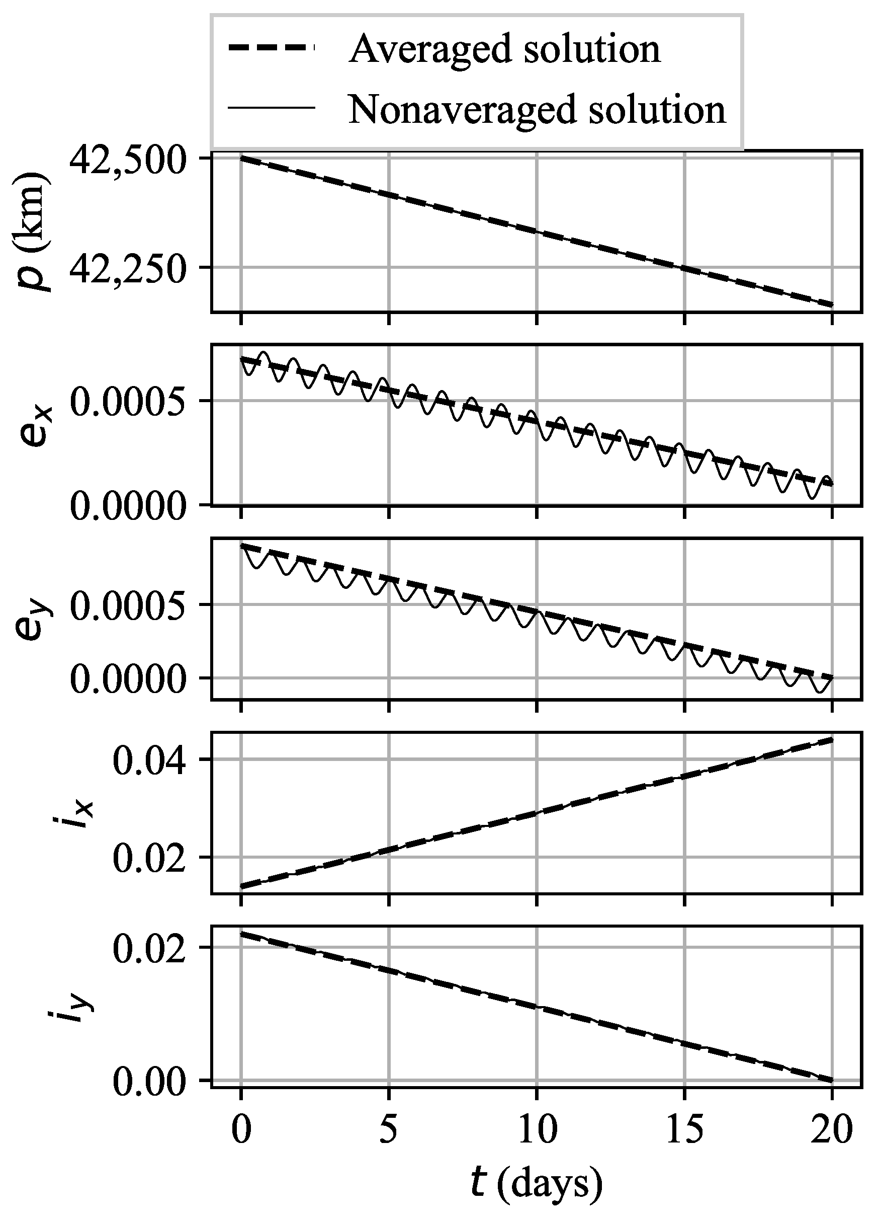
Figure 4 illustrates the evolution of the averaged and nonaveraged osculating values of the modified equinoctial elements, influenced by the achieved optimal control of the averaging stage. The nonaveraged values of
and
experience substantial changes during the transfer, despite their corresponding averaged elements remaining at a value of zero. The final and target equinoctial elements are depicted in
Table 4. This example highlights that, in certain instances, the disparity between the averaged and nonaveraged trajectories can be substantial, necessitating corrections to the averaged optimal control in the nonaveraged scenario to meet the target orbit constraint within nonaveraged dynamics.
5.3. Comparison with Pontryagin Maximum Principle Control
It should be noted that the thrust accelerations obtained for Cases A and B are computed under the assumption that the control is a periodic function over the eccentric longitude. The question is whether the optimal control in a general class of piecewise-continuous function is close to a periodic function or not. To find it out, the obtained control is compared with the one calculated using the well-known Pontryagin maximum principle.
The optimal control in the class of piecewise-continuous functions is constructed as follows. The optimal control problem is posed in the classical Bolza formulation for a transfer between two fixed phase vectors for a fixed transfer time:
where
and
are the position and velocity of the spacecraft;
is the thrust acceleration;
T is a given time; and
,
,
, and
are the initial and boundary constraints.
From a practical standpoint, the considered optimal control problem is equivalent to maximizing the spacecraft’s mass at the final time assuming a fixed jet propulsion power. In fact, since jet power equals
, where
represents the exhaust velocity and
is the thrust force, then
After integrating the derived equations, one gets
so minimizing
J leads to maximizing
.
The Hamiltonian function is written as follows:
where
and
are the conjugate variables. Maximizing
H with respect to
gives
, so the extended equations are
The problem of finding an optimal solution is reduced to finding the initial values of the conjugate variables
and
such that propagating the above extended system of equations with
and
gives the target values
and
.
The derived boundary value problem can be solved using the differential parameter continuation method with respect to the gravitational parameter, described, for example, in [
32]. To utilize this method, it is necessary to determine the number of revolutions around the center of attraction. This is typically performed manually by managing the resulting fuel costs or maximum values of control variables. It is worth noting that the averaging method presented earlier does not require the specification of the number of revolutions. Moreover, while the differential continuation method is regular, it does involve integrating a system of differential equations, which includes the inversion of a matrix on the right-hand side. When dealing with a large number of revolutions, this method may face convergence issues, which are further complicated by the need to manually select the number of turns. This issue is not present in the proposed averaging method.
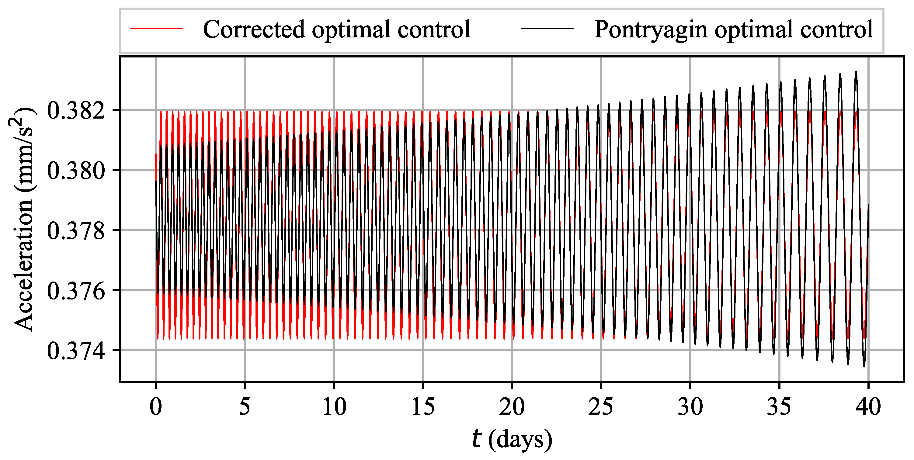
The Pontryagin maximum principle, in conjunction with the method of differential parameter continuation, was used to address the problems of Cases A and B, resulting in the acquisition of Pontryagin extremals (the control functions that meet the necessary conditions for optimality). The acceleration control profiles that were derived from the maximum principle and the two-staged optimization method are compared in
Figure 5 and
Figure 6 for Cases A and B, respectively. It is evident that in Case A, the accelerations achieved are almost the same. The resulting values of the objective are
= 30,205
for the presented technique and
= 30,204
for the maximum principle, the relative difference
. However, in Case B, while the accelerations appear to be similar, the spectrum of the Pontryagin optimal control is gradually changing over time. The objective values are also similar: 247,366
for the two-stage optimization method and 247,365
for the maximum principle with a relative difference equal to
.
6. Conclusions and Further Research
This study presents a novel approach to generate an initial estimation for low-thrust optimization problems. This method utilizes the closed-form approximation of the averaged dynamics of a nearly circular orbit, enabling the conversion of the multirevolution orbital transfer problem into a moderately sized nonlinear programming problem. The solution to this problem is found to be near the optimal control. Applying this newly developed approach, two test energy-optimal control problems were successfully solved. It was determined that for transfers between closely situated near-circular orbits, the obtained control serves as a precise initial estimate: further optimization in the nonaveraged model only results in minor modifications.
Numerous aspects of the introduced method are being considered for additional investigation. For instance, the search for optimal low-thrust acceleration is conducted among functions with a constant Fourier spectrum. However, the energy-optimal thrust acceleration found in the nonaveraged model through indirect methods possesses a spectrum that progressively changes over time. In such scenarios, a potential modification to the introduced method could involve searching for thrust acceleration with a spectrum that is piecewise constant. This would cause the number of optimization variables to increase N-fold, but it would remain finite and relatively low.
Another question is the ability to account for various disturbances to the equations of motion: nonsphericity of the central body, other planets’ attraction, atmospheric drag, solar radiation pressure, etc. Accounting for them in the model of motion will remove the ability to analytically average the equations and thus parameterize the control. One of the ideas is to approximate disturbing accelerations with periodic functions like it is done for the low-thrust acceleration. This approximation might be quite accurate for disturbing accelerations with a slowly changing magnitude and direction, such as the gravitational attraction of other bodies, solar radiation pressure, and atmospheric drag. Unfortunately, nonsphericity gravity field effects that have a major effect on low orbits are hard to represent this way. The question of accounting for these disturbances is a subject of further research.
Author Contributions
Conceptualization, K.S. and M.S.; Methodology, K.S.; Software, K.S. and M.S; Validation, K.S., M.S. and A.T.; Formal Analysis, K.S.; Investigation, A.T.; Resources, M.S. and A.T.; Data Curation, M.S.; Writing–Original Draft Preparation, K.S.; Writing–Review & Editing, M.S. and A.T.; Visualization, K.S.; Supervision, M.S.; Project Administration, M.S. All authors have read and agreed to the published version of the manuscript.
Funding
This research received no external funding.
Institutional Review Board Statement
Not applicable.
Data Availability Statement
Data are contained within the article.
Conflicts of Interest
The authors declare no conflict of interest.
Nomenclature
| a | semimajor axis |
| E | eccentric anomaly |
| e | eccentricity |
| F | eccentric longitude |
| vector of the low-thrust acceleration |
| f | magnitude of the low-thrust acceleration |
| circumferential component of the low-thrust acceleration |
| normal component of the low-thrust acceleration |
| radial component of the low-thrust acceleration |
| i | inclination |
| L | true longitude |
| m | spacecraft mass |
| P | jet propulsion power |
| p, , , , | modified equinoctial elements |
| T | time of flight |
| exhaust velocity |
| vector of modified equinoctial elements |
| vector of averaged modified equinoctial elements |
| cosine coefficient, Fourier series of the low-thrust acceleration |
| sine coefficient, Fourier series of the low-thrust acceleration |
| mean longitude |
| gravitational parameter of the central body |
| longitude of the ascending node |
| argument of periapsis |
References
- Conway, B. (Ed.) Spacecraft Trajectory Optimization; Cambridge University Press: Cambridge, UK, 2010. [Google Scholar] [CrossRef]
- Shirazi, A.; Ceberio, J.; Lozano, J.A. Spacecraft trajectory optimization: A review of models, objectives, approaches and solutions. Prog. Aerosp. Sci. 2018, 102, 76–98. [Google Scholar] [CrossRef]
- Bryson, A.E.; Ho, Y. Applied Optimal Control, 1st ed.; Routledge: New York, NY, USA, 1975; 496p. [Google Scholar]
- Lewis, A.D. The Maximum Principle of Pontryagin in Control and in Optimal Control. Handouts for the Course Taught at the Universitat Politecnica de Catalunya. 2006. Available online: https://citeseerx.ist.psu.edu/document?repid=rep1&type=pdf&doi=22a4c6ba37caf048029197bd5689a51ac9a57ac0 (accessed on 24 October 2023).
- Petropoulos, A.; Russell, R. Low-thrust transfers using primer vector theory and a second-order penalty method. In Proceedings of the AIAA/AAS Astrodynamics Specialist Conference and Exhibit, Honolulu, HI, USA, 18–21 August 2008. [Google Scholar]
- Oshima, K.; Campagnola, S.; Yanao, T. Global search for low-thrust transfers to the Moon in the planar circular restricted three-body problem. Celest. Mech. Dyn. Astr. 2017, 128, 303–322. [Google Scholar] [CrossRef]
- Pérez-Palau, D.; Epenoy, R. Fuel optimization for low-thrust Earth–Moon transfer via indirect optimal control. Celest. Mech. Dyn. Astr. 2018, 130, 21. [Google Scholar] [CrossRef]
- Kluever, C.A.; Oleson, S.R. Direct Approach for Computing Near-Optimal Low-Thrust Earth-Orbit Transfers. J. Spacecr. Rocket. 1998, 35, 509–515. [Google Scholar] [CrossRef]
- Betts, J.T. Very low-thrust trajectory optimization using a direct SQP method. J. Comput. Appl. Math. 2000, 120, 27–40. [Google Scholar] [CrossRef]
- Topputo, F.; Zhang, C. Survey of direct transcription for low-thrust space trajectory optimization with applications. Abstr. Appl. Anal. 2014, 1–15. [Google Scholar] [CrossRef]
- Oshima, K. Regularized direct method for low–thrust trajectory optimization: Minimum–fuel transfer between cislunar periodic orbits. Adv. Space Res. 2023, 72, 2051–2063. [Google Scholar] [CrossRef]
- Wu, D.; Guo, X.; Jiang, F.; Baoyin, H. Atlas of optimal low-thrust rephasing solutions in circular orbit. J. Guid. Control. Dyn. 2023, 46, 856–870. [Google Scholar] [CrossRef]
- Wu, D.; Cheng, L.; Gong, S.; Baoyin, H. Approximate time-optimal low-thrust rendezvous solutions between circular orbits. Aerosp. Sci. Technol. 2022, 113, 108011. [Google Scholar] [CrossRef]
- Lin, X.; Zhang, G.; Ma, H. Optimal low-thrust linearized elliptic orbit rendezvous considering the communication window. Acta Astronaut. 2022, 197, 14–22. [Google Scholar] [CrossRef]
- Gurfil, P. Spacecraft rendezvous using constant-magnitude low thrust. J. Guid. Control. Dyn. 2023, 46, 2183–2191. [Google Scholar] [CrossRef]
- Huang, A.-Y.; Luo, Y.-Z.; Li, H.-N. Optimization of low-thrust rendezvous between circular orbits via thrust-switch strategy. J. Guid. Control. Dyn. 2022, 45, 1143–1152. [Google Scholar] [CrossRef]
- Kolda, T.G.; Lewis, R.M.; Torczon, V. Optimization by direct search: New perspectives on some classical and modern methods. SIAM Rev. 2003, 45, 385–482. [Google Scholar] [CrossRef]
- Zhu, Z.; Gan, Q.; Yang, X.; Gao, Y. Solving fuel-optimal low-thrust orbital transfers with bang-bang control using a novel continuation technique. Acta Astronaut. 2017, 137, 98–113. [Google Scholar] [CrossRef]
- Shirazi, A. Adaptive estimation of distribution algorithms for low-thrust trajectory optimization. J. Spacecr. Rocket. 2023, 60, 1585–1596. [Google Scholar] [CrossRef]
- Chen, Q.; Qiao, D.; Wen, C. Minimum-fuel low-thrust trajectory optimization via reachability analysis and convex programming. J. Guid. Control. Dyn. 2021, 44, 1036–1043. [Google Scholar] [CrossRef]
- Benedikter, B.; Zavoli, A.; Wang, Z.; Pizzurro, S.; Cavallini, E. Convex approach to covariance control with application to stochastic low-thrust trajectory optimization. J. Guid. Control. Dyn. 2022, 45, 2061–2075. [Google Scholar] [CrossRef]
- Izzo, D.; Blazquez, E.; Ferede, R.; Origer, S.; De Wagter, C.; de Croon, G.C.H.E. Optimality principles in spacecraft neural guidance and control. arXiv 2023, arXiv:2305.13078. [Google Scholar] [CrossRef]
- Dachwald, B. Optimization of very-low-thrust trajectories using evolutionary neurocontrol. Acta Astronaut. 2005, 57, 175–185. [Google Scholar] [CrossRef][Green Version]
- Petukhov, V.G. Optimization of multi-orbit transfers between noncoplanar elliptic orbits. Cosm. Res. 2004, 42, 250–268. [Google Scholar] [CrossRef]
- Tarzi, Z.; Speyer, J.; Wirz, R. Fuel optimum low-thrust elliptic transfer using numerical averaging. Acta Astronaut. 2013, 86, 95–118. [Google Scholar] [CrossRef]
- Guelman, M.; Kogan, A.; Gipsman, A. Asymptotic optimization of very long, low thrust propelled inter-orbital maneuvers. Acta Astronaut. 2000, 47, 489–502. [Google Scholar] [CrossRef]
- da Silva Fernandes, S.; das Chagas Carvalho, F. A first-order analytical theory for optimal low-thrust limited-power transfers between arbitrary elliptical coplanar orbits. Math. Probl. Eng. 2008, 2008, 525930. [Google Scholar] [CrossRef]
- Kitamura, K.; Yamada, K.; Shima, T. Minimum energy coplanar orbit transfer of geostationary spacecraft using time-averaged Hamiltonian. Acta Astronaut. 2019, 160, 270–279. [Google Scholar] [CrossRef]
- Hudson, J.S.; Scheeres, D.J. Reduction of low-thrust continuous controls for trajectory dynamics. J. Guid. Control. Dyn. 2009, 32, 780–787. [Google Scholar] [CrossRef]
- Hudson, J.S.; Scheeres, D.J. Orbital targeting using reduced eccentric anomaly low-thrust coefficients. J. Guid. Control. Dyn. 2011, 34, 820–831. [Google Scholar] [CrossRef]
- Walker, M.J.H.; Ireland, B.; Owens, J. A set of modified equinoctial orbit elements. Celest. Mech. 1985, 36, 409–419. [Google Scholar] [CrossRef]
- Petukhov, V.G. Optimization of interplanetary trajectories for spacecraft with ideally regulated engines using the continuation method. Cosm. Res. 2008, 46, 219–232. [Google Scholar] [CrossRef]
| Disclaimer/Publisher’s Note: The statements, opinions and data contained in all publications are solely those of the individual author(s) and contributor(s) and not of MDPI and/or the editor(s). MDPI and/or the editor(s) disclaim responsibility for any injury to people or property resulting from any ideas, methods, instructions or products referred to in the content. |
© 2023 by the authors. Licensee MDPI, Basel, Switzerland. This article is an open access article distributed under the terms and conditions of the Creative Commons Attribution (CC BY) license (https://creativecommons.org/licenses/by/4.0/).


