
Effect of Engine Design Parameters on the Climate Impact of Aircraft: A Case Study Based on Short-Medium Range Mission


Abstract
:1. Introduction
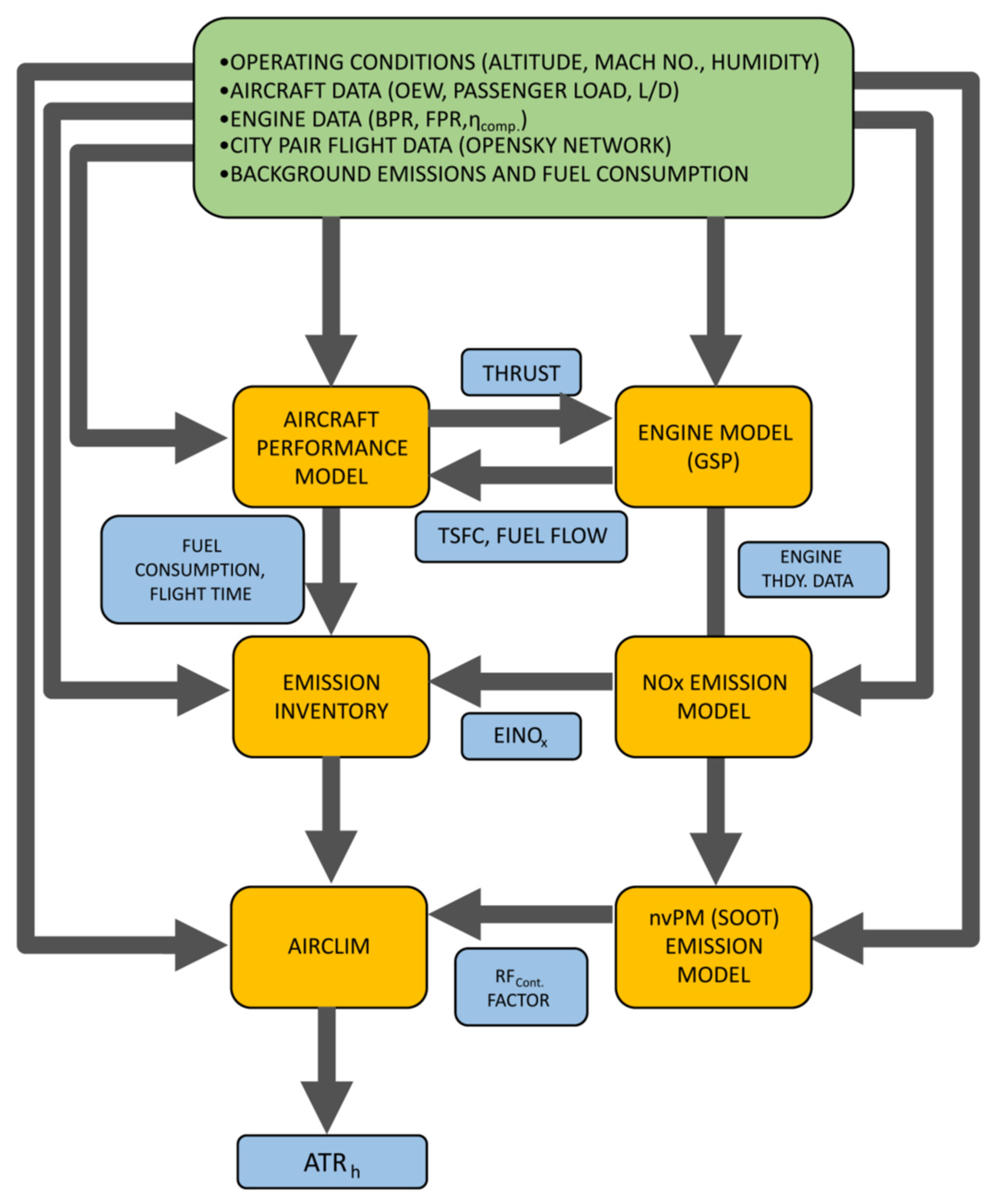
2. Methodology
2.1. Aircraft Performance Model
2.2. Engine Performance Model
2.3. Emission Models
2.3.1. Rich-Burn Combustor Emission Modeling
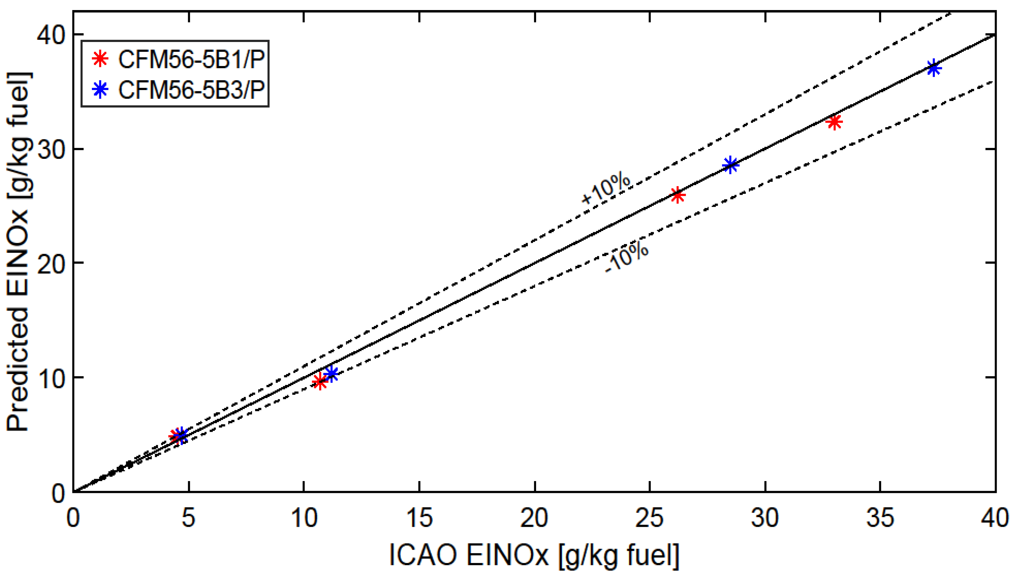
Rich-Burn EINOx Model
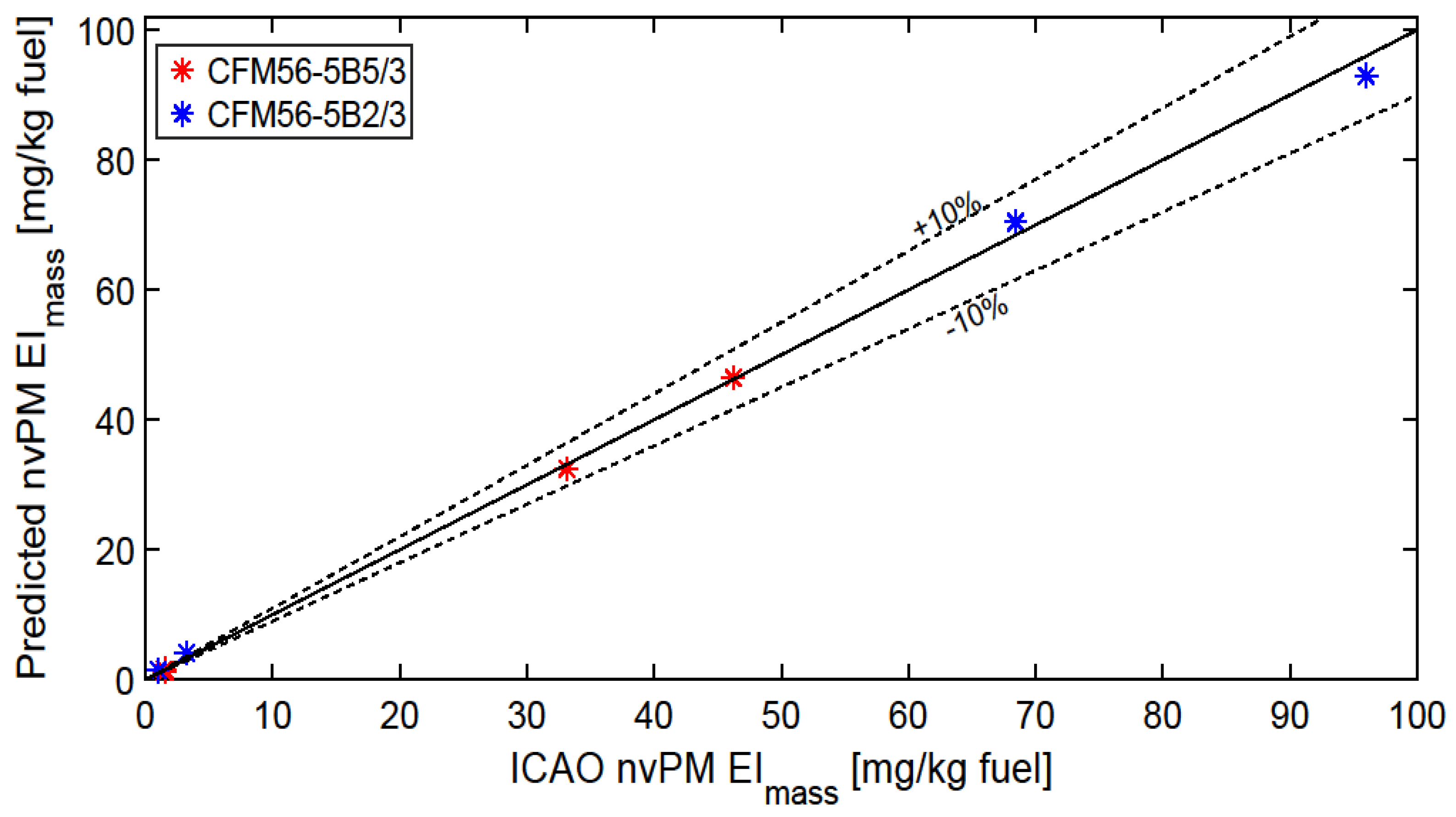
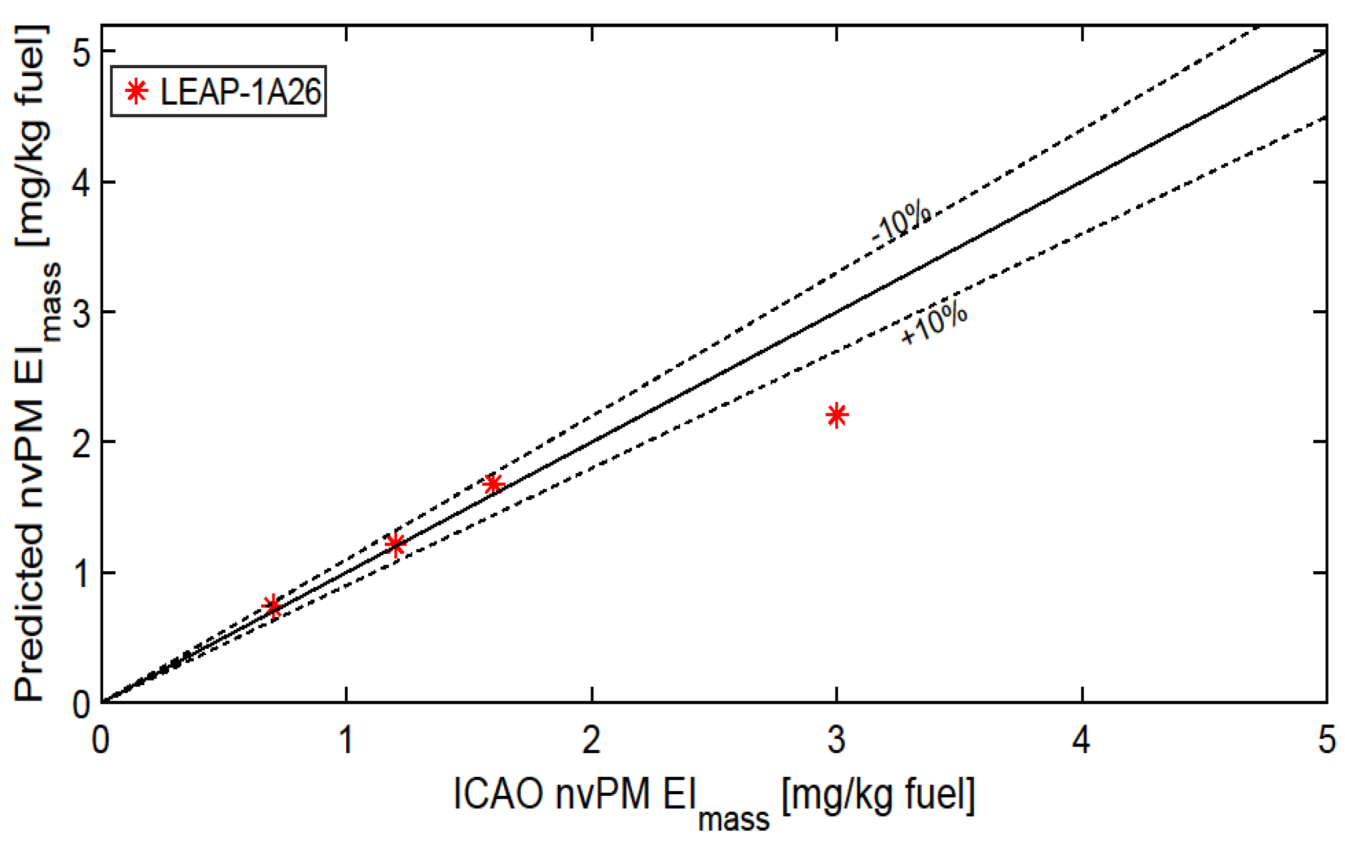
Rich-Burn nvPM Model
2.3.2. Lean-Burn TAPS-II Emissions Modeling
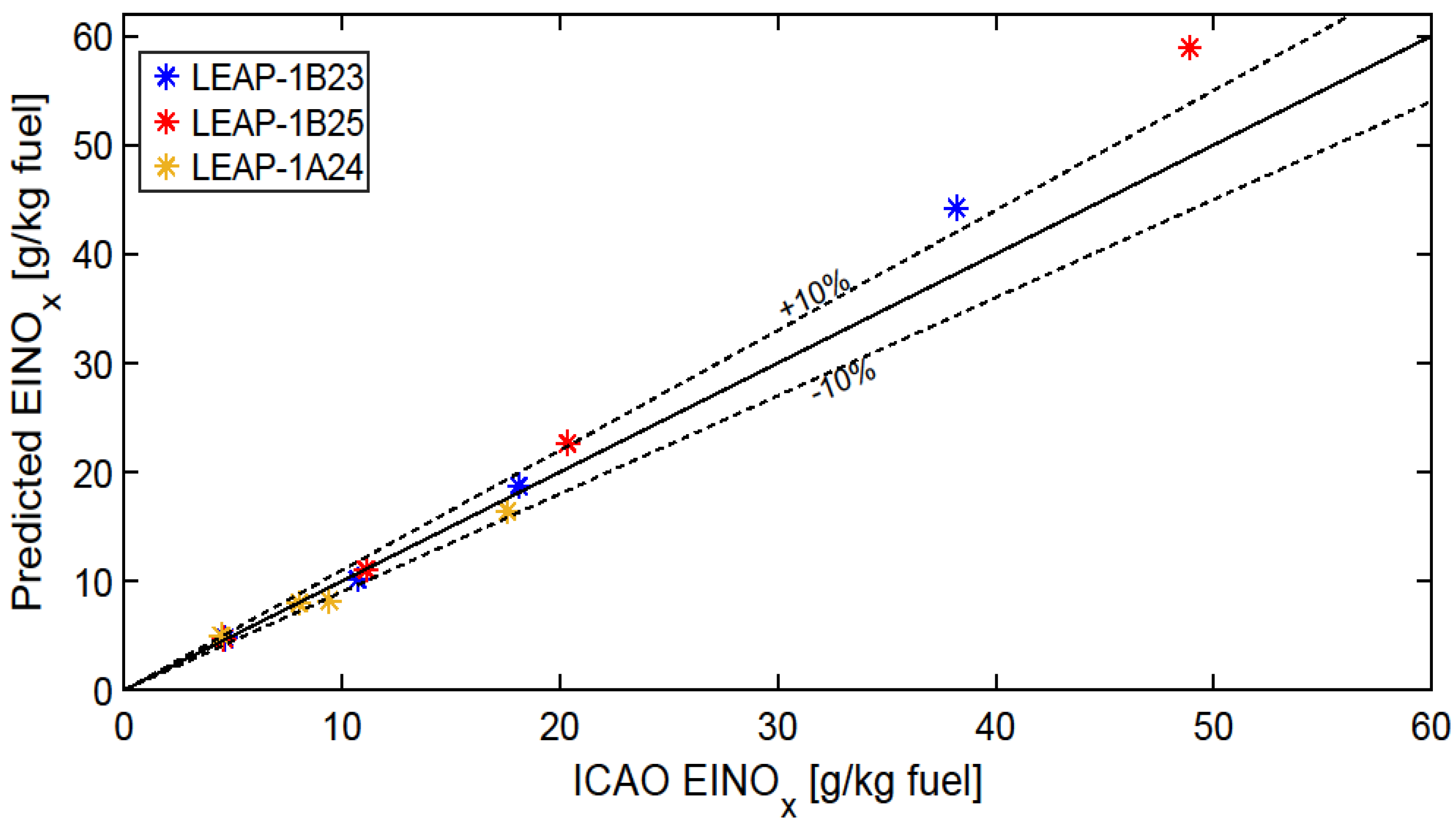
Lean-Burn TAPS-II EINOx Model
Lean-Burn TAPS nvPM Model
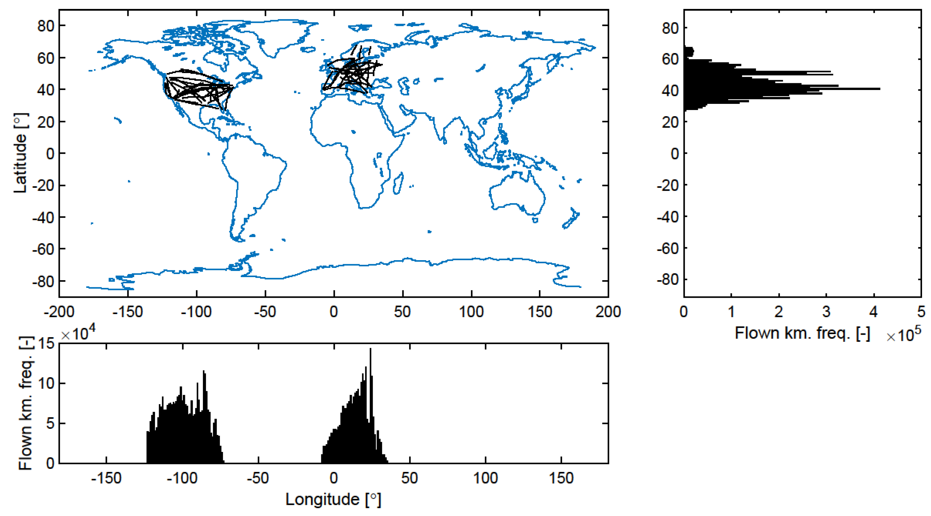
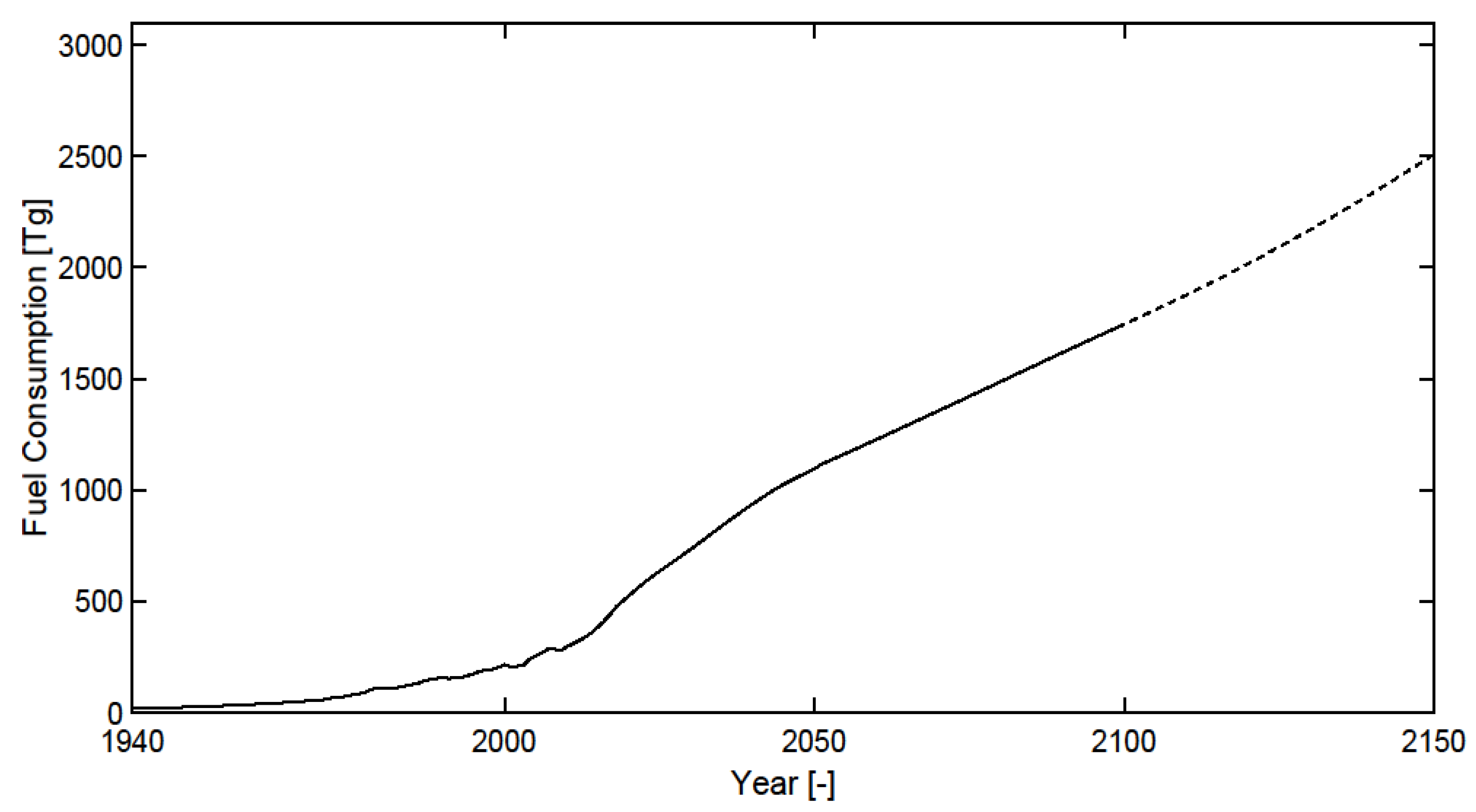
2.4. The Emission Inventory
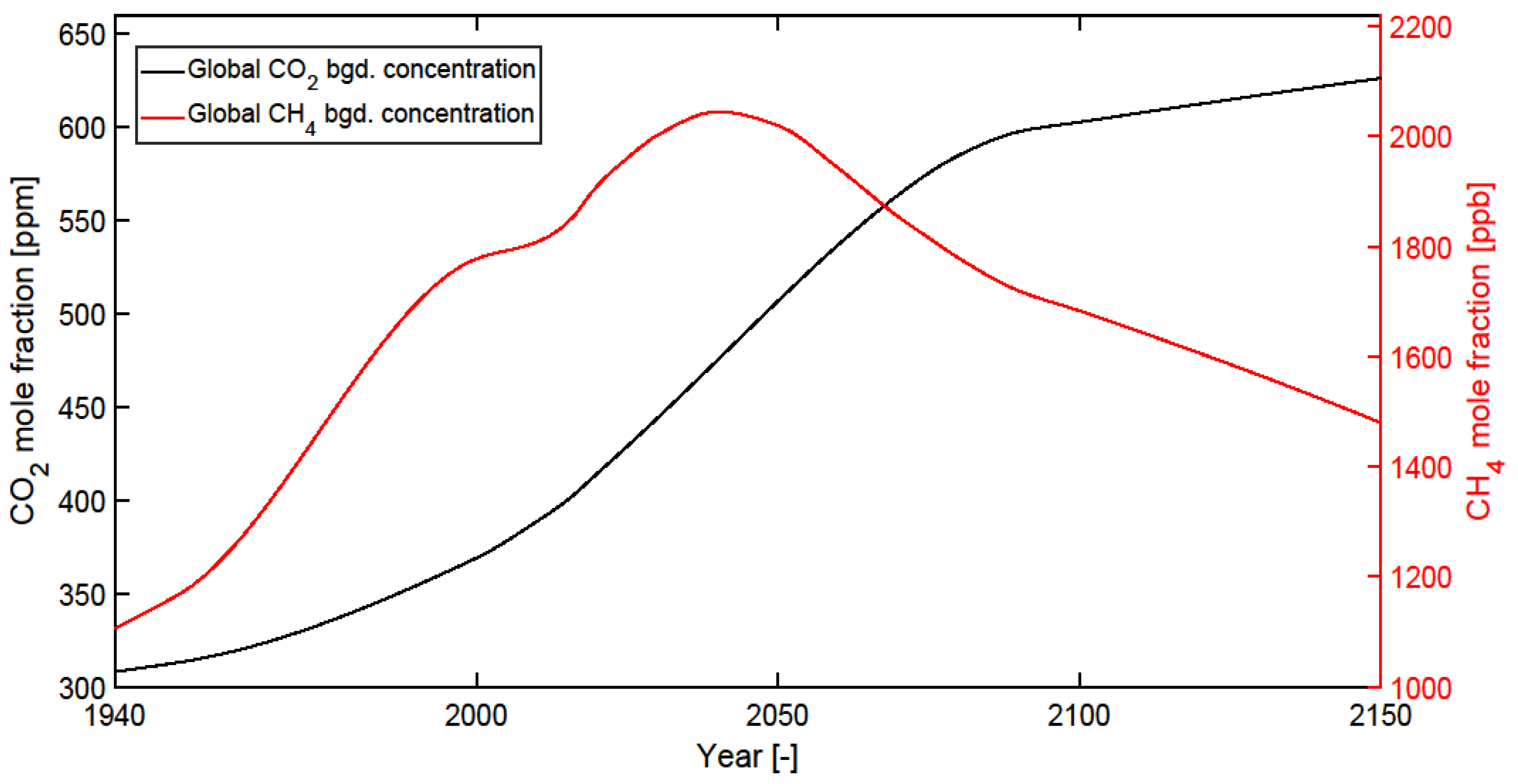
2.5. Climate Assessment Model
2.6. Modelling Uncertainties
3. Results and Discussion
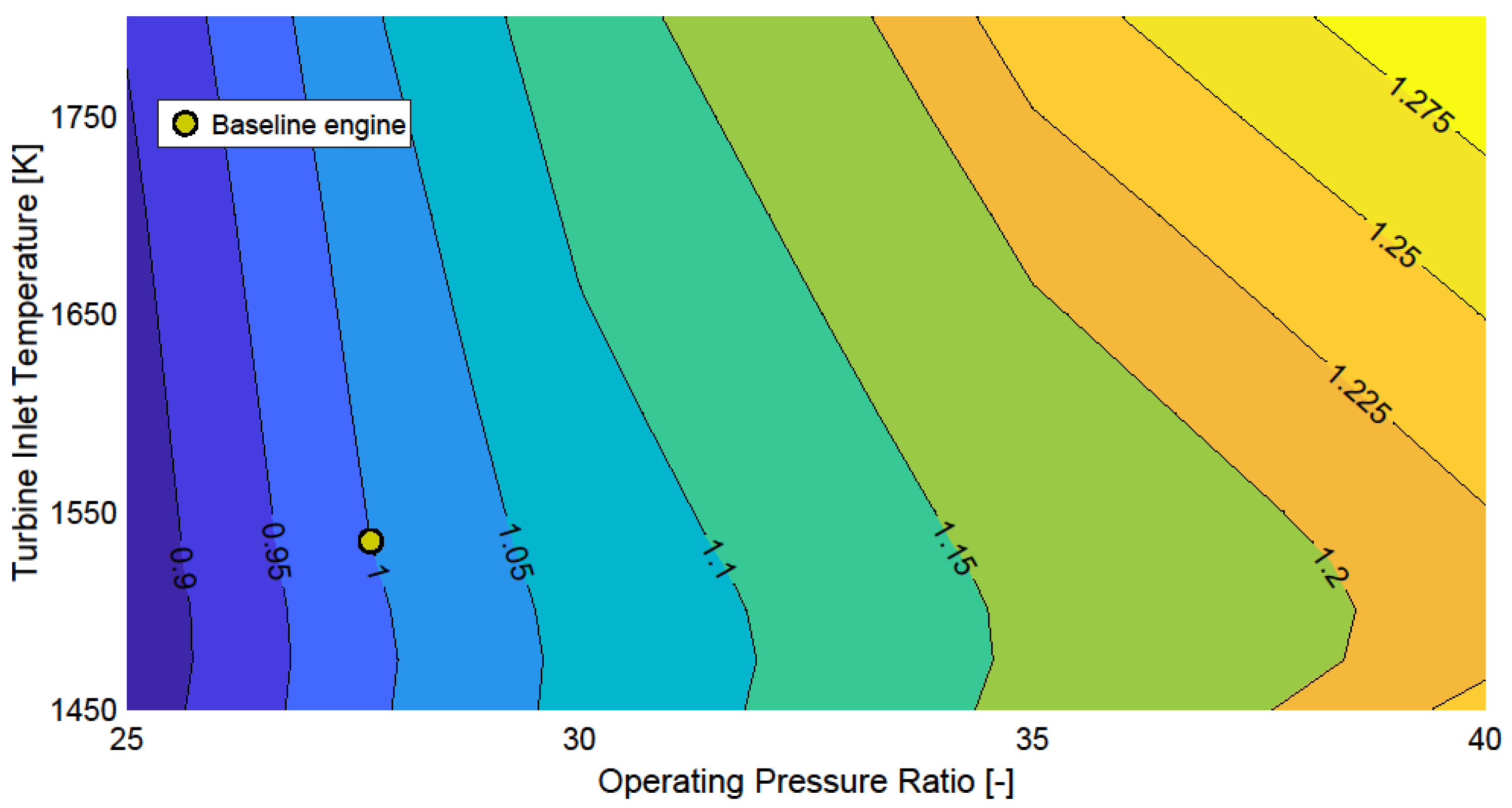
3.1. Resultant Parameters for the Baseline Engine Configuration
3.2. Parametric Results
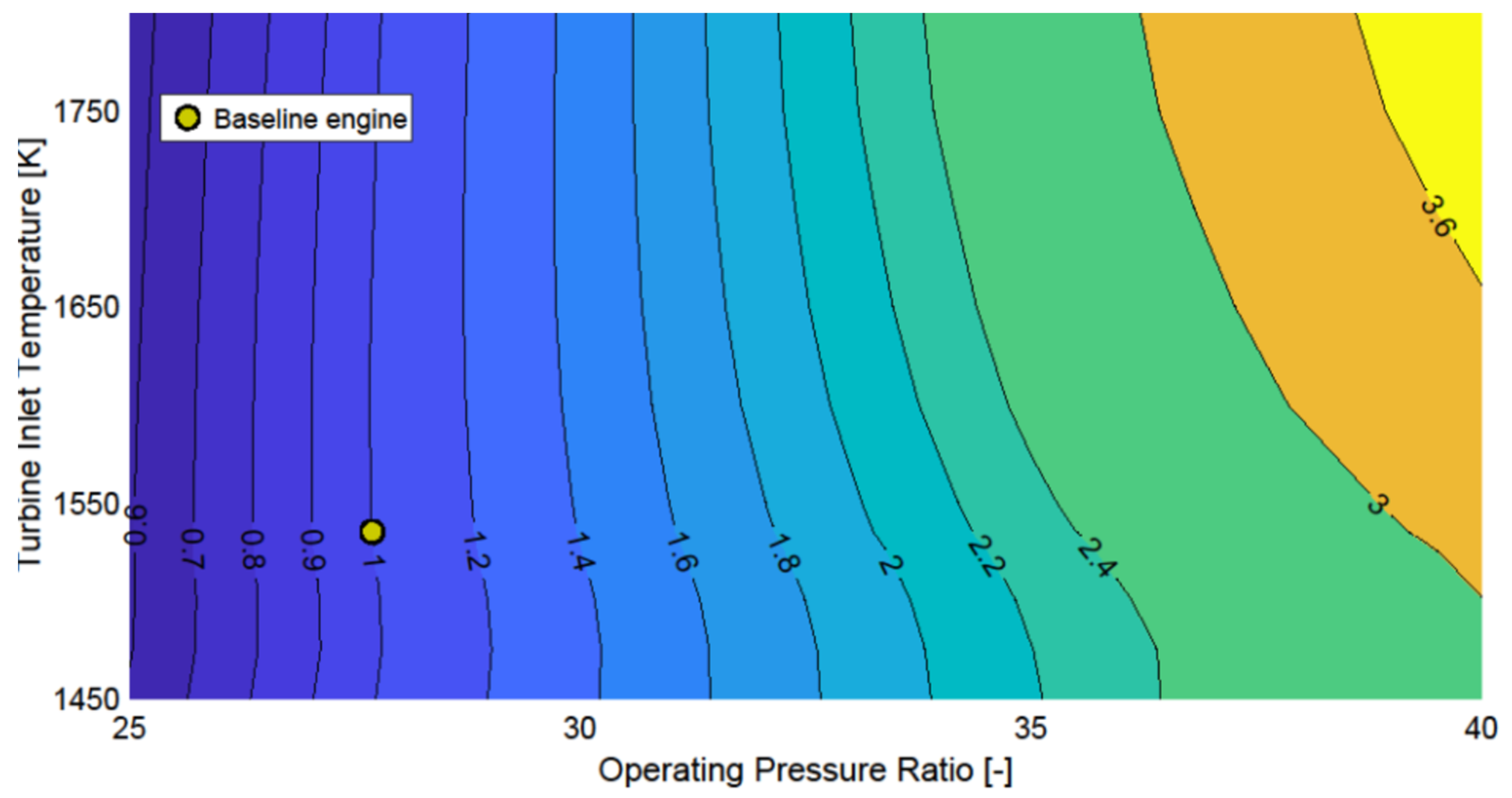
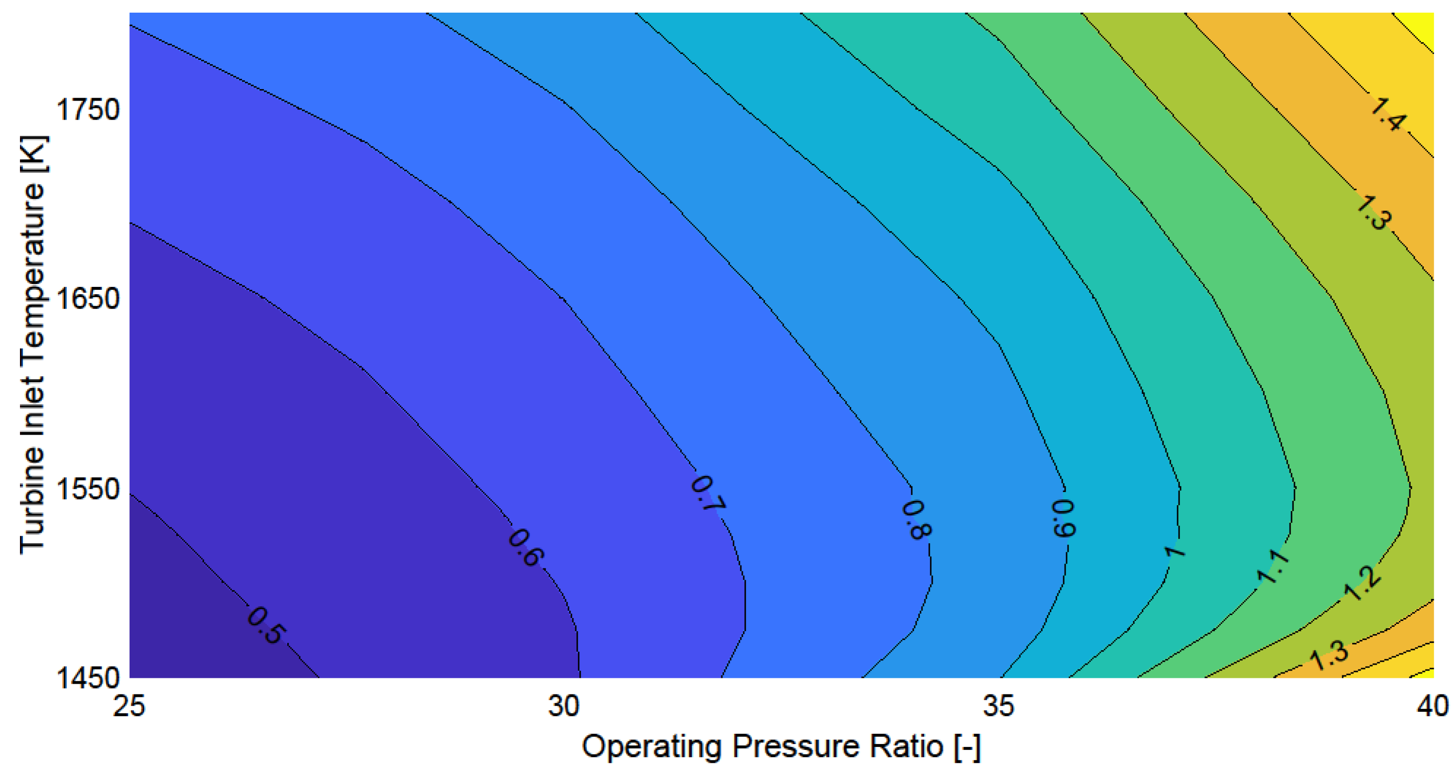
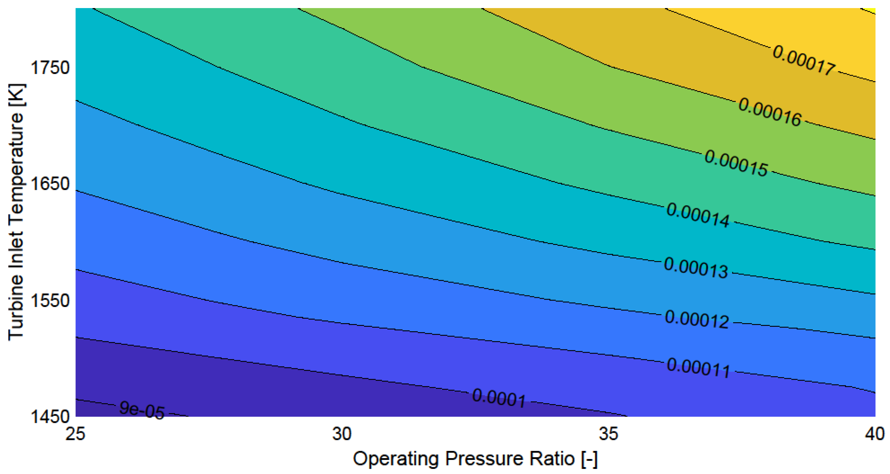
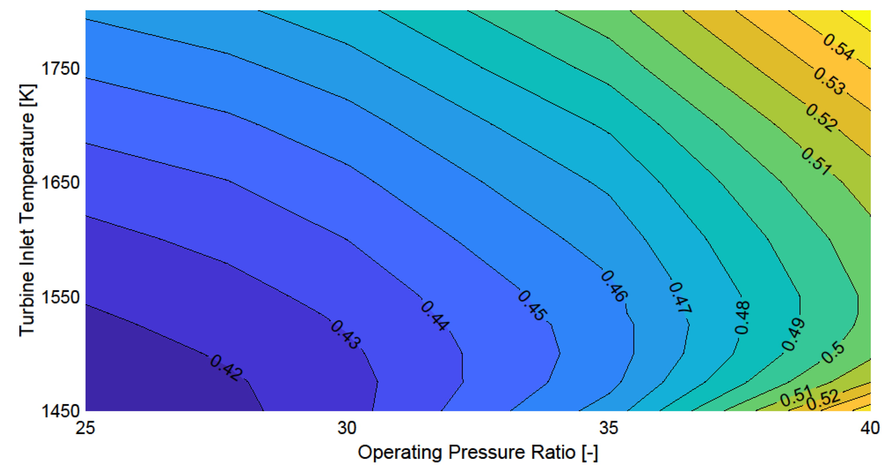
3.2.1. Rich Burn Combustor Configurations
Variation in Fuel Consumption
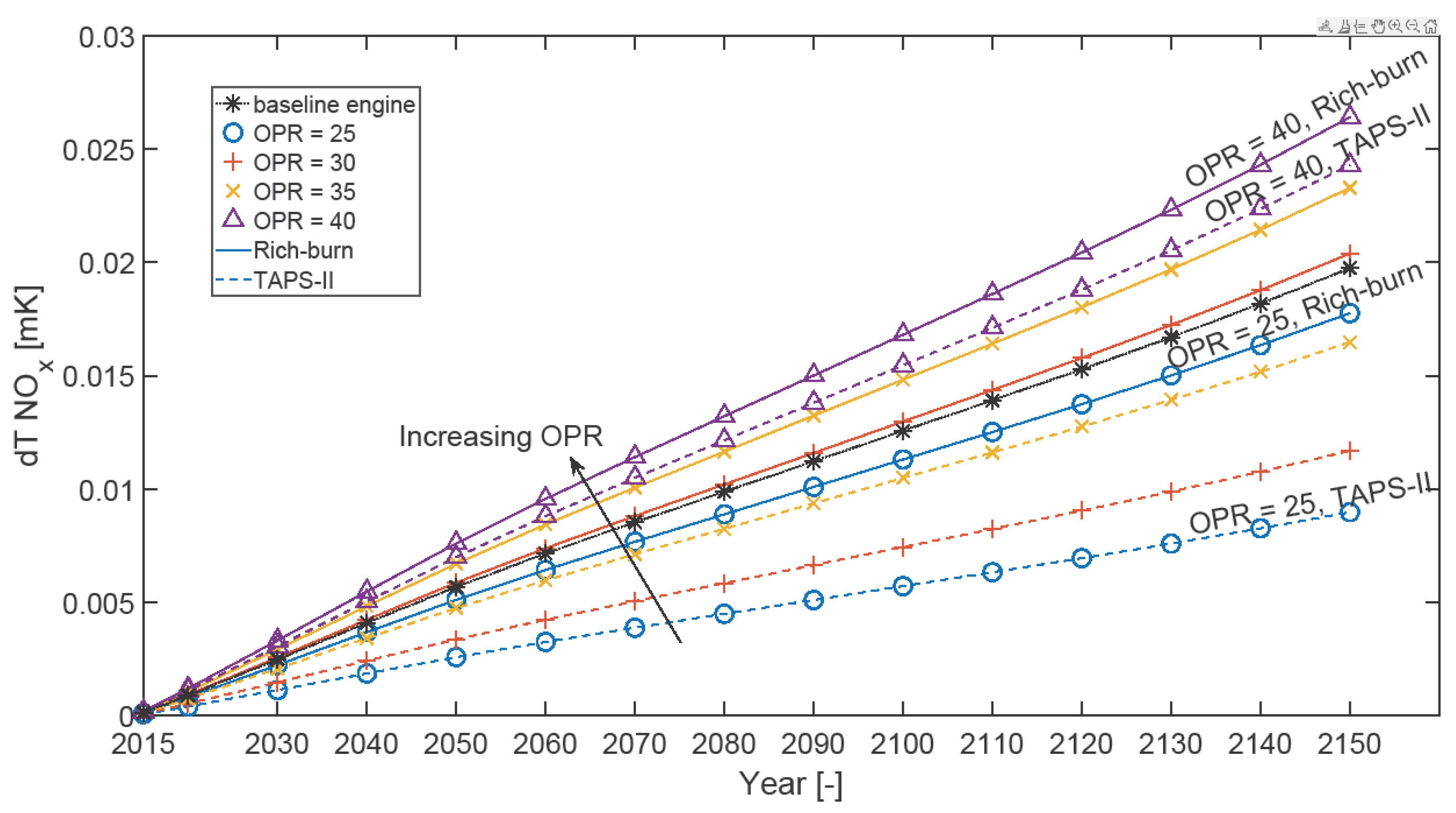
Variation of Emissions
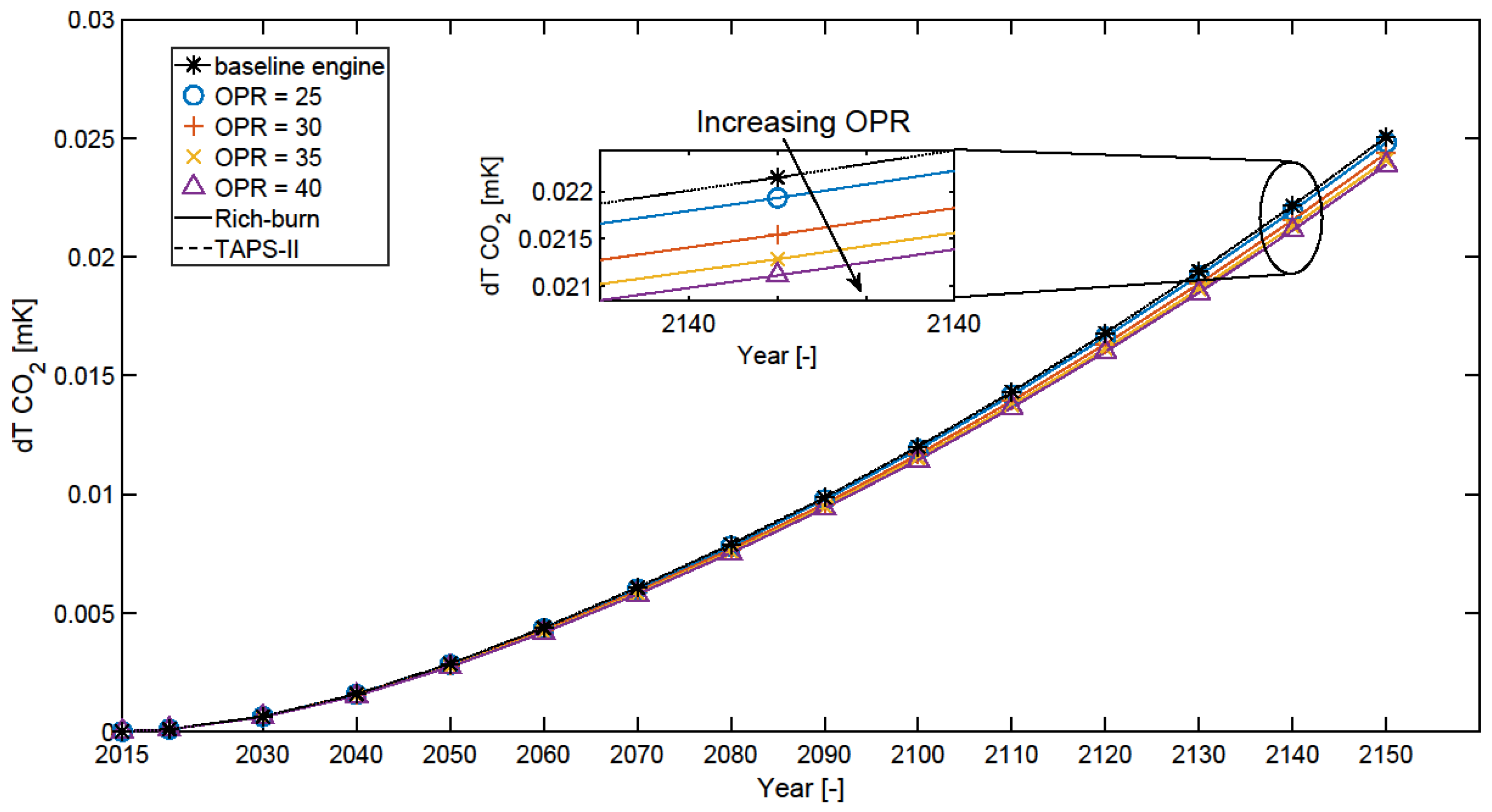
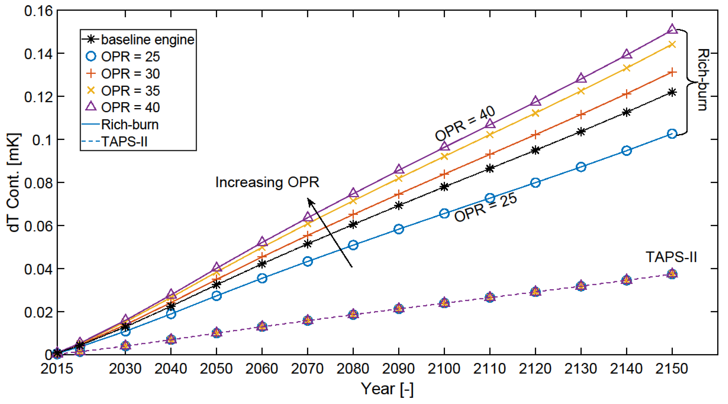
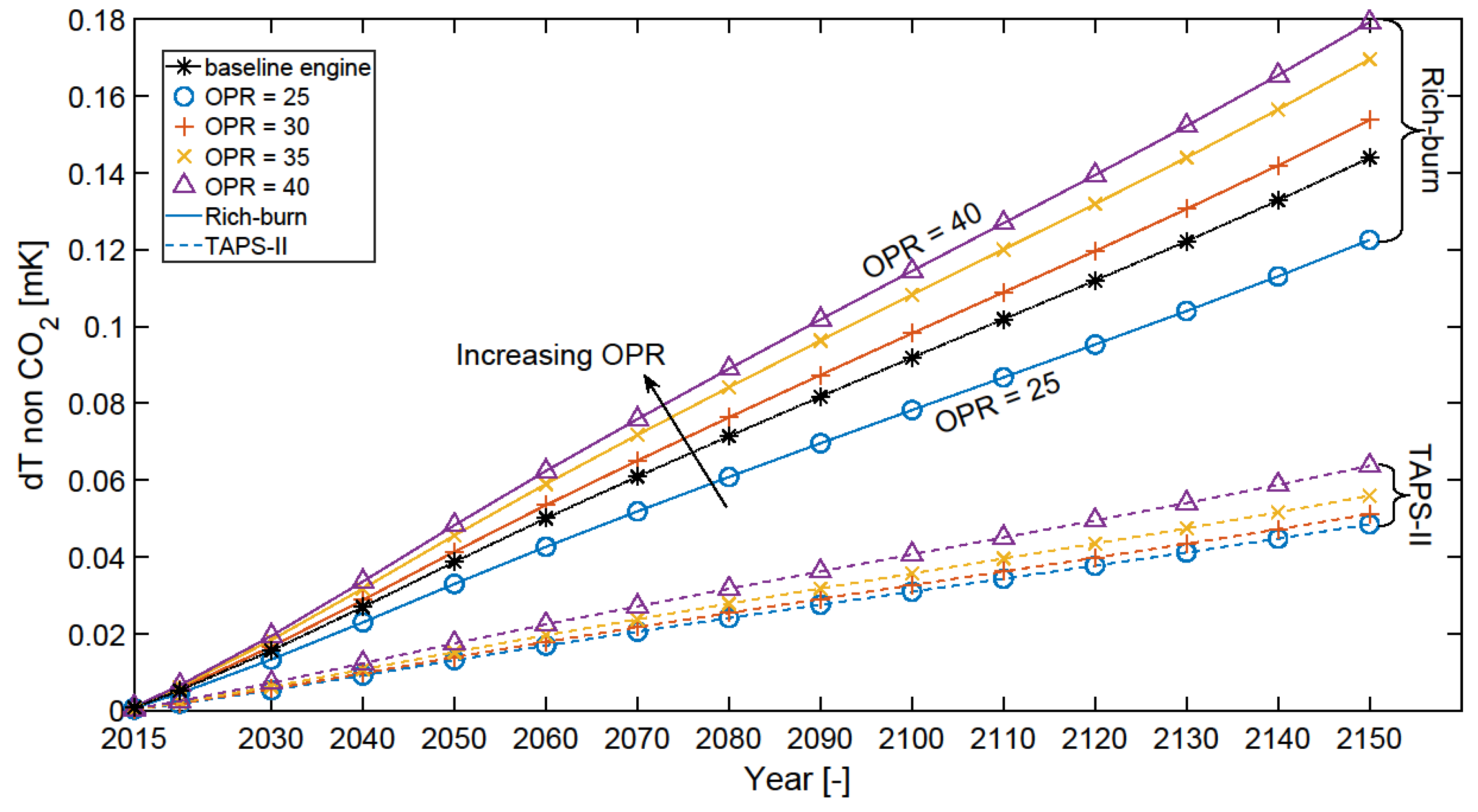
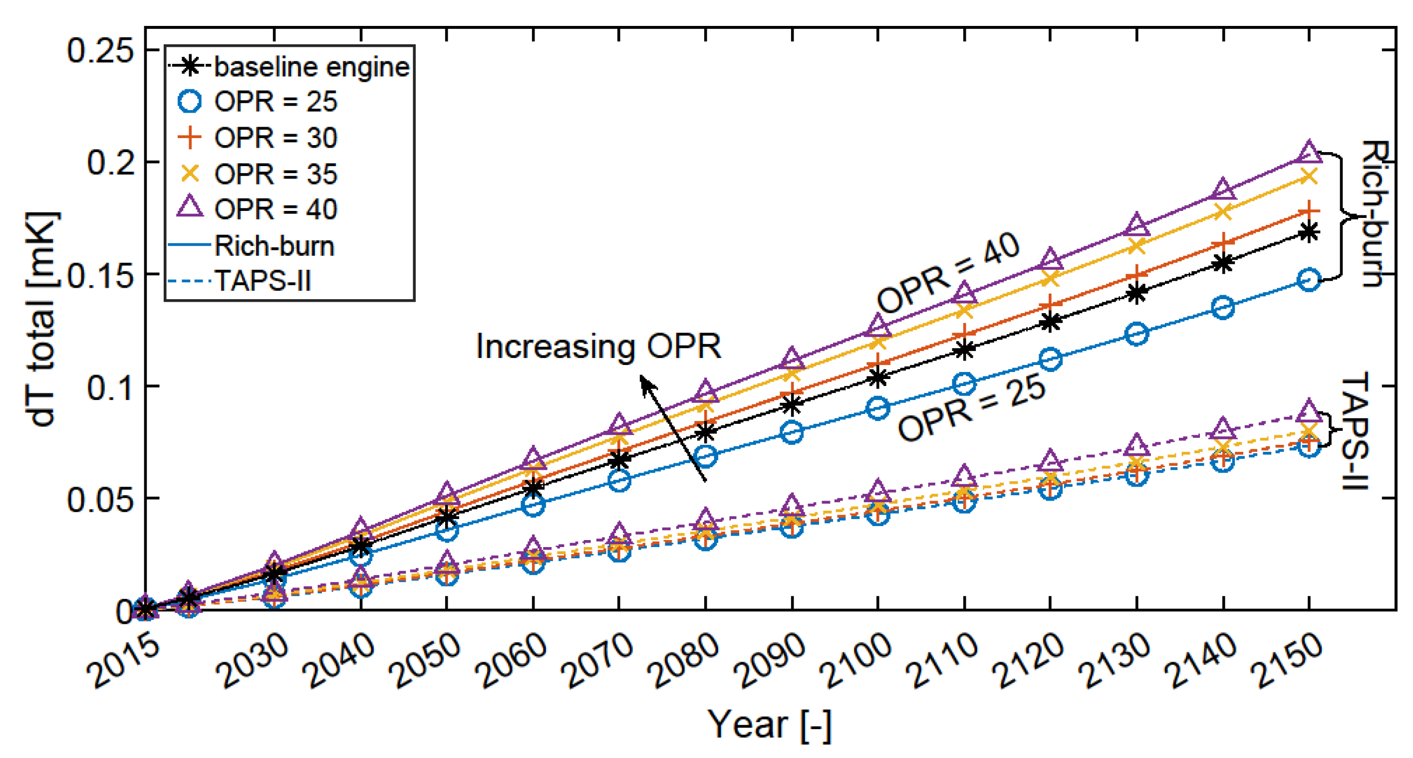
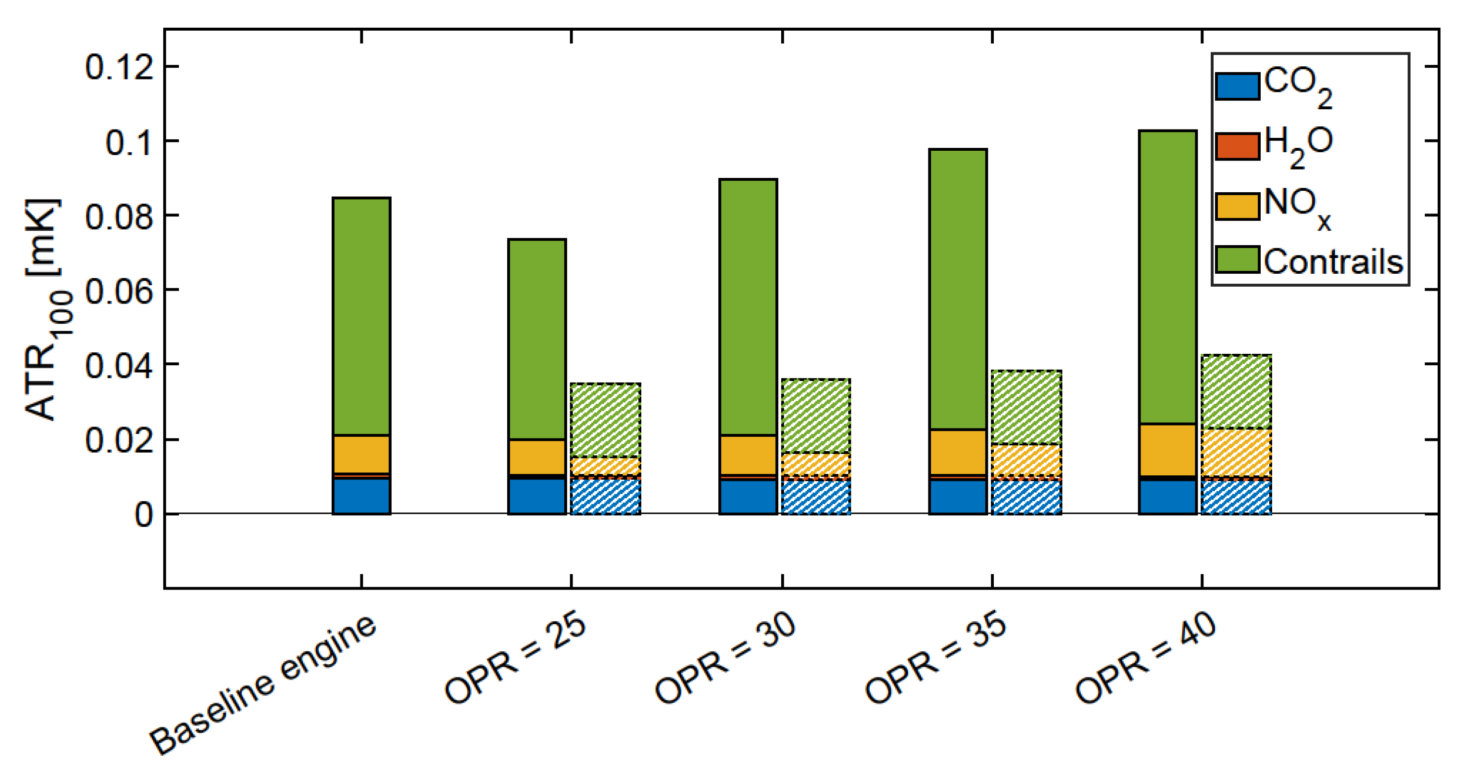
Variation of ATR100
3.2.2. Lean-Burn Combustor Configurations
Variation of Emissions
Variation of ATR100
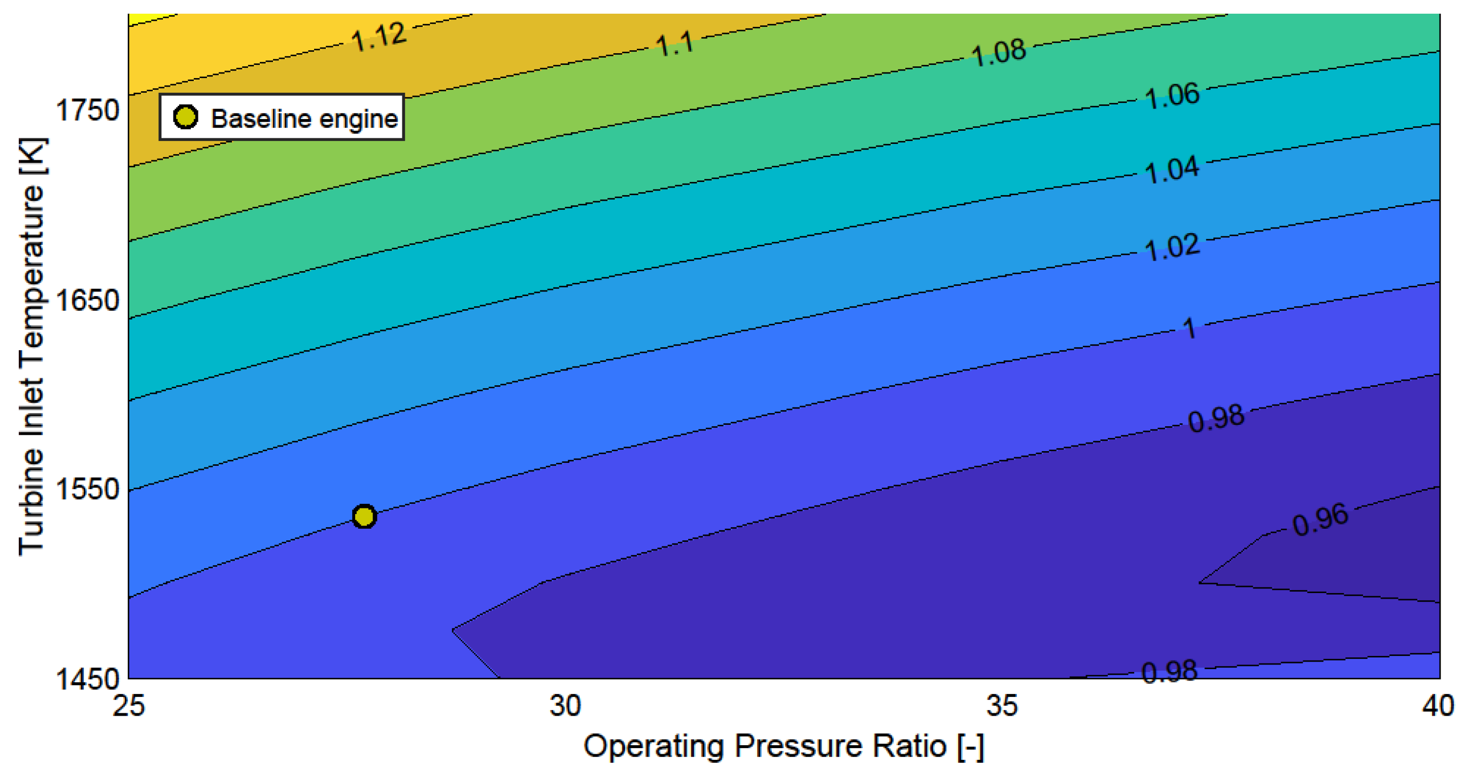
3.3. Climate Impact Analysis for Engines with a Minimal Fuel Burn
4. Conclusions
Author Contributions
Funding
Data Availability Statement
Conflicts of Interest
Abbreviations
| ACARE | Advisory Council for Aviation Research and Innovation in Europe |
| ATR | Average Temperature Response |
| BPR | Bypass Ratio |
| CCM | Climate Chemistry Model |
| CORSIA | Carbon Offsetting and Reduction Scheme for International Aviation |
| EI | Emission Index |
| ERF | Effective Radiative Forcing |
| FAR | Fuel-to-Air ratio |
| GSP | Gas Turbine Simulation Program |
| GWP | Global Warming Potential |
| ICAO | International Civil Aviation Organization |
| LB | Lean Burn |
| LEAP | Leading Edge Aviation Propulsion |
| LTO | Landing and Take-off Cycle |
| nvPM | Non-volatile Particulate Matter |
| OEW | Operating Empty Weight |
| OPR | Operating Pressure Ratio |
| PMO | Primary-mode Ozone |
| RF | Radiative Forcing |
| RQL | Rich-Burn Quick-Quench Lean-burn |
| SLS | Static Sea-Level |
| TAPS | Twin Annular Premixed Swirler |
| TIT | Turbine Inlet Temperature |
| TSFC | Thrust-Specific Fuel Consumption |
| Symbols | |
| ATR100 | Average Temperature Response over 100 years |
| ATRbaseline | ATR for the baseline configuration |
| BaselineParam. | Baseline Engine Design Parameter |
| dcruise | Cruise Distance |
| EImass,cruise | nvPM Cruise Mass Emission Index |
| EImass,SLS | nvPM SLS Mass Emission Index |
| nvPM SLS Mass Emission Index for pilot Operation | |
| nvPM SLS Mass Emission Index for pilot + main Operation | |
| EINOx,cruise | Cruise NOx Emission Index |
| EINOx,SLS | SLS NOx Emission Index |
| SLS NOx Emission Index for pilot Operation | |
| SLS NOx Emission Index for pilot + main Operation | |
| EInum,cruise | nvPM Cruise Number Emission Index |
| EIspecies | Species Emission Index |
| FARcruise | Cruise FAR |
| FARSLS | SLS FAR |
| Favg.aircraft | Average Aircraft Cruise Thrust |
| Favg.engine | Average Engine Cruise Thurst |
| Fengine | Engine Thrust Level |
| Engine Design Species Climate Sensitivity over a Time Horizon of h Years | |
| h | Atmospheric Humidity |
| hcruise | Cruise Altitude |
| L/D | Lift-to-Drag Ratio |
| m | FAR-Term Exponent in P3–T3 Correlation |
| n | Pressure-Term Exponent in P3–T3 Correlation |
| Pt3 | Combustor Inlet Pressure |
| Pt3,cruise | Cruise Combustor Inlet Pressure |
| Pt3,SLS | SLS Combustor Inlet Pressure |
| RFcontr. | Contrail Radiative Forcing |
| tcruise | Cruise Time |
| Tt3 | Combustor Inlet Temperature |
| a | Intake Air Mass Flow Rate |
| Wapp.payload | Apparent Payload Weight |
| Wend | Aircraft Weight at the End of Cruise |
| Wf,cruise | Cruise Fuel Weight |
| f,cruise | Cruise Fuel Flow Rate |
| WNOx | NOx Emission Weight |
| Wspecies,cruise | Weight of Emission Species |
| Wstart | Aircraft Weight at the Beginning of Cruise |
| ΔATRspec. | Change in Species ATR |
| ΔDesignParam. | Change in Engine Design Parameter |
| Δpn | Relative Change in nvPM Number Emissions |
| ΔRFcontr | Change in Contrail Radiative Forcing |
| ΔTs.contr | Temperature Change due to Contrail-Induced Radiative Forcing |
| ν | nvPM Number-to-Mass Emission Index Ratio |
| νp | nvPM Number-to-Mass Emission Index Ratio for pilot Operation |
| νp+m | nvPM Number-to-Mass Emission Index Ratio for pilot + main Operation |
Appendix A
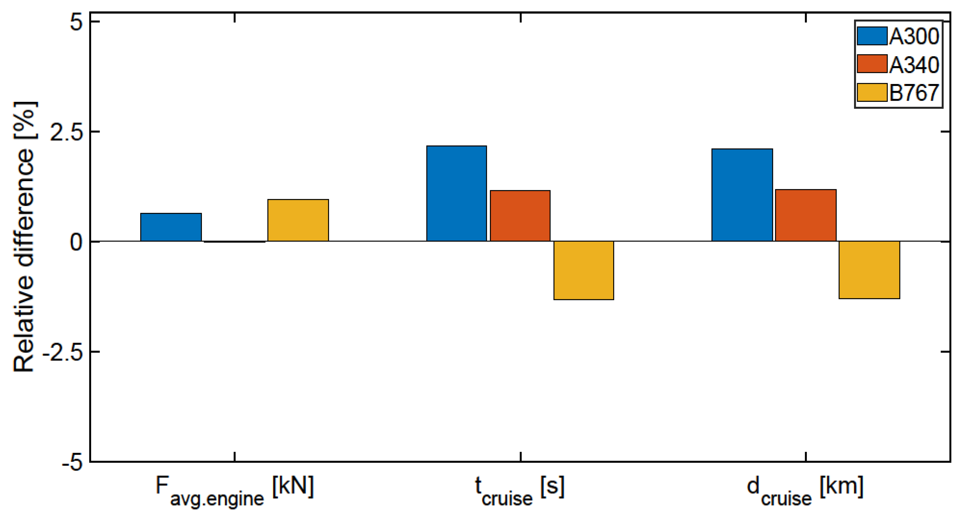
Appendix A.1. Validation Cases of the Aircraft Performance Model

| Aircraft | Cruise Mach No. | Cruise Distance | Cruise Fuel Weight | Operating Empty Weight | Apparent Payload Weight | Lift-to-Drag Ratio | Thrust-Specific Fuel Consumption |
|---|---|---|---|---|---|---|---|
| M | dcruise | Wf,cruise | OEW | Wapp.payload | L/D | TSFC | |
| (-) | (km) | (kg) | (kg) | (kg) | (-) | (kg/Ns) | |
| A300-600R | 0.8 | 4587 | 27,852 | 89,813 | 32,519.23 | 15.51 | 1.637 × 10⁻⁵ |
| A340-642 | 0.82 | 13,405 | 127,337 | 181,100 | 45,015.38 | 19 | 1.526 × 10⁻⁵ |
| B767-300ERW | 0.82 | 10,619 | 59,168 | 93,032 | 30,636.48 | 18.31 | 1.632 × 10⁻⁵ |
Appendix A.2. PIANO Simulations of the A320neo Aircraft for TAPS-II Exponent Determination
| Cruise Operating Conditions | Cruise Distance (Km) | Wf,cruise (kg) | WNOx (g) | EINOx (g/kg fuel) |
|---|---|---|---|---|
| hcruise = 34,000 ft Mach no. = 0.775 | 1025.1 | 2920.4 | 16.79 | 5.75 |
| hcruise = 36,000 ft Mach no. = 0.775 | 2906.41 | 7703.3 | 43.07 | 5.6 |
| hcruise = 38,000 ft Mach no. = 0.775 | 2110.6 | 5115 | 27.20 | 5.32 |
References
- Lee, D.S.; Fahey, D.W.; Skowron, A.; Allen, M.R.; Burkhardt, U.; Chen, Q.; Doherty, S.J.; Freeman, S.; Forster, P.M.; Fuglestvedt, J. The contribution of global aviation to anthropogenic climate forcing for 2000 to 2018. Atmos. Environ. 2021, 244, 117834. [Google Scholar] [CrossRef] [PubMed]
- Wilcox, L.J.; Shine, K.P.; Hoskins, B.J. Radiative forcing due to aviation water vapour emissions. Atmos. Environ. 2012, 63, 1–13. [Google Scholar] [CrossRef]
- Stevenson, D.S.; Doherty, R.M.; Sanderson, M.G.; Collins, W.J.; Johnson, C.E.; Derwent, R.G. Radiative forcing from aircraft NOx emissions: Mechanisms and seasonal dependence. J. Geophys. Res. Atmos. 2004, 109, D17. [Google Scholar] [CrossRef]
- Köhler, M.O.; Rädel, G.; Shine, K.P.; Rogers, H.L.; Pyle, J.A. Latitudinal variation of the effect of aviation NOx emissions on atmospheric ozone and methane and related climate metrics. Atmos. Environ. 2013, 64, 1–9. [Google Scholar] [CrossRef]
- Dahlmann, K.; Grewe, V.; Frömming, C.; Burkhardt, U. Can we reliably assess climate mitigation options for air traffic scenarios despite large uncertainties in atmospheric processes? Transp. Res. Part D Transp. Environ. 2016, 46, 40–55. [Google Scholar] [CrossRef]
- Kärcher, B. Formation and radiative forcing of contrail cirrus. Nat. Commun. 2018, 9, 1824. [Google Scholar] [CrossRef]
- Schumann, U.; Graf, K. Aviation-induced cirrus and radiation changes at diurnal timescales. J. Geophys. Res. Atmos. 2013, 118, 2404–2421. [Google Scholar] [CrossRef]
- Burkhardt, U.; Kärcher, B. Global radiative forcing from contrail cirrus. Nat. Clim. Chang. 2011, 1, 54. [Google Scholar] [CrossRef]
- Heymsfield, A.; Baumgardner, D.; DeMott, P.; Forster, P.; Gierens, K.; Kärcher, B. Contrail Microphysics. Bull. Am. Meteorol. Soc. 2010, 91, 465–472. [Google Scholar] [CrossRef]
- Burkhardt, U.; Bock, L.; Bier, A. Mitigating the contrail cirrus climate impact by reducing aircraft soot number emissions. npj Clim. Atmos. Sci. 2018, 1, 37. [Google Scholar] [CrossRef]
- Lacis, A.A.; Schmidt, G.A.; Rind, D.; Ruedy, R.A. Atmospheric CO2: Principal Control Knob Governing Earth’s Temperature. Science 2010, 330, 356–359. [Google Scholar] [CrossRef] [PubMed]
- Frömming, C.; Grewe, V.; Brinkop, S.; Jöckel, P.; Haslerud, A.S.; Rosanka, S.; van Manen, J.; Matthes, S. Influence of the actual weather situation on aviation climate effects: The REACT4C Climate Change Functions. Atmos. Chem. Phys. 2021, 21, 9151–9172. [Google Scholar] [CrossRef]
- Gauss, M.; Isaksen, I.S.A.; Lee, D.S.; Søvde, O.A. Impact of aircraft NOx emissions on the atmosphere tradeoffs to reduce the impact. Atmos. Chem. Phys. 2006, 6, 1529–1548. [Google Scholar] [CrossRef]
- Advisory Council for Aviation Research and Innovation (ACARE). Flight 2050 Europe’s Vision for Aviation; European Commission: Brussels, Belgium, 2011. [Google Scholar]
- Grewe, V.; Gangoli Rao, A.; Grönstedt, T.; Xisto, C.; Linke, F.; Melkert, J.; Middel, J.; Ohlenforst, B.; Blakey, S.; Christie, S.; et al. Evaluating the climate impact of aviation emission scenarios towards the Paris agreement including COVID-19 effects. Nat. Commun. 2021, 12, 3841. [Google Scholar] [CrossRef] [PubMed]
- United Nations Framework Convention on Climate Change (UNFCCC). Adoption of the Paris Agreement; United Nations: New York, NY, USA, 2015. [Google Scholar]
- Kyprianidis, K.G.; Dahlquist, E. On the trade-off between aviation NOx and energy efficiency. Appl. Energy 2017, 185, 1506–1516. [Google Scholar] [CrossRef]
- Yin, F.; Rao, A.G. Performance analysis of an aero engine with inter-stage turbine burner. Aeronaut. J. 2017, 121, 1605–1626. [Google Scholar] [CrossRef]
- Thoma, E.M.; Grönstedt, T.; Zhao, X. Quantifying the Environmental Design Trades for a State-of-the-Art Turbofan Engine. Aerospace 2020, 7, 148. [Google Scholar] [CrossRef]
- Perpignan, A.A.V.; Talboom, M.G.; Levy, Y.; Rao, A.G. Emission Modeling of an Interturbine Burner Based on Flameless Combustion. Energy Fuels 2018, 32, 822–838. [Google Scholar] [CrossRef]
- Sehra, A.K.; Whitlow, W. Propulsion and power for 21st century aviation. Prog. Aerosp. Sci. 2004, 40, 199–235. [Google Scholar] [CrossRef]
- Freeman, S.; Lee, D.S.; Lim, L.L.; Skowron, A.; De León, R.R. Trading off Aircraft Fuel Burn and NOx Emissions for Optimal Climate Policy. Environ. Sci. Technol. 2018, 52, 2498–2505. [Google Scholar] [CrossRef]
- Durdina, L.; Brem, B.T.; Setyan, A.; Siegerist, F.; Rindlisbacher, T.; Wang, J. Assessment of Particle Pollution from Jetliners: From Smoke Visibility to Nanoparticle Counting. Environ. Sci. Technol. 2017, 51, 3534–3541. [Google Scholar] [CrossRef] [PubMed]
- Kaiser, S.; Schmitz, O.; Ziegler, P.; Klingels, H. The Water-Enhanced Turbofan as Enabler for Climate-Neutral Aviation. Appl. Sci. 2022, 12, 12431. [Google Scholar] [CrossRef]
- Kaiser, S.; Seitz, A.; Donnerhack, S.; Lundbladh, A. Composite Cycle Engine Concept with Hectopressure Ratio. J. Propuls. Power 2016, 32, 1413–1421. [Google Scholar] [CrossRef]
- Owen, B.; Anet, J.G.; Bertier, N.; Christie, S.; Cremaschi, M.; Dellaert, S.; Edebeli, J.; Janicke, U.; Kuenen, J.; Lim, L.; et al. Review: Particulate Matter Emissions from Aircraft. Atmosphere 2022, 13, 1230. [Google Scholar] [CrossRef]
- Stickles, R.; Barrett, J. TAPS II Technology Final Report—Technology Assessment Open Report. DTFAWA-10-C-00046, Washington DC, USA, 2013. Available online: https://www.faa.gov/sites/faa.gov/files/about/office_org/headquarters_offices/apl/TAPS_II_Public_Final_Report.pdf (accessed on 1 October 2023).
- Grewe, V.; Stenke, A. AirClim: An efficient tool for climate evaluation of aircraft technology. Atmos. Chem. Phys. 2008, 8, 4621–4639. [Google Scholar] [CrossRef]
- Norman, P.D.; Lister, D.H.; Lecht, M.; Madden, P.; Park, K.; Penanhoat, O.; Plaisance, C.; Renger, K. Development of the Technical Basis for a New Emissions Parameter Covering the Whole Aircraft Operation: NEPAIR; Final Technical Report No. NEPAIR/WP4/WPR/01; European Commission: Luxembourg, 2003. [Google Scholar]
- Schäfer, M.; Strohmeier, M.; Lenders, V.; Martinovic, I.; Wilhelm, M. Bringing up OpenSky: A large-scale ADS-B sensor network for research. In Proceedings of the IPSN-14 Proceedings of the 13th International Symposium on Information Processing in Sensor Networks, Berlin, Germany, 15–17 April 2014; pp. 83–94. [Google Scholar]
- Sun, J.; Hoekstra, J.M.; Ellerbroek, J. OpenAP: An Open-Source Aircraft Performance Model for Air Transportation Studies and Simulations. Aerospace 2020, 7, 104. [Google Scholar] [CrossRef]
- Anderson, J.D.; Bowden, M.L. Introduction to Flight; McGraw-Hill Education: New York, NY, USA, 2021. [Google Scholar]
- Visser, W.; Broomhead, M. GSP: A Generic Object-Oriented Gas Turbine Simulation Environment; National Aerospace Laboratory NLR: Amsterdam, The Netherlands, 2000. [Google Scholar]
- Antoine, N.E.; Kroo, I.M. Aircraft optimization for minimal environmental impact. J. Aircr. 2004, 41, 790–797. [Google Scholar] [CrossRef]
- Döpelheuer, A.; Lecht, M. Influence of engine performance on emission characteristics. RTO AVT Symposium on Gas Turbine Engine Combustion, Emissions and Alternative Fuels. Lisbon, Portugal, 12–16 October; 1998. Available online: https://api.semanticscholar.org/CorpusID:97575598 (accessed on 1 October 2023).
- Foust, M.; Thomsen, D.; Stickles, R.; Cooper, C.; Dodds, W. Development of the GE Aviation Low Emissions TAPS Combustor for Next Generation Aircraft Engines. In Proceedings of the 50th AIAA Aerospace Sciences Meeting Including the New Horizons Forum and Aerospace Exposition, Nashville, Tennessee, 9–12 January 2012. [Google Scholar] [CrossRef]
- Megill, L.; Deck, K.; Grewe, V. A systematic approach to select a suitable climate metric for aviation policy and aircraft design. 2023; preprint. [Google Scholar] [CrossRef]
- Meinshausen, M.; Nicholls, Z.R.J.; Lewis, J.; Gidden, M.J.; Vogel, E.; Freund, M.; Beyerle, U.; Gessner, C.; Nauels, A.; Bauer, N.; et al. The shared socio-economic pathway (SSP) greenhouse gas concentrations and their extensions to 2500. Geosci. Model Dev. 2020, 13, 3571–3605. [Google Scholar] [CrossRef]
- Kroon, R. Aviation Emission Inventory: A Contemporized Bottom-Up Emission Inventory for the Year 2019. Master’s Thesis, Delft University of Technology, Delft, The Netherlands, 2022. [Google Scholar]
- Lefebvre, A.H.; Ballal, D.R. Gas Turbine Combustion: Alternative Fuels and Emissions, 3rd ed.; CRC Press: Boca Raton, FL, USA, 2010. [Google Scholar]
- Warnatz, J.; Maas, U.; Dibble, R.W. Combustion: Physical and Chemical Fundamentals, Modeling and Simulation, Experiments, Pollutant Formation, 4th ed.; Springer: Berlin/Heidelberg, Germany, 2006. [Google Scholar]
- Jenkinson, L.R.; Simpkin, P.; Rhodes, D.; Royce, R. Civil Jet Aircraft Design; Arnold: London, UK, 1999; Volume 338. [Google Scholar]


| Config. | Fuel Consumption | NOx Emissions | Mean EINOx | 020) | 1014) | ATR100 |
|---|---|---|---|---|---|---|
| (t(Fuel)) | (t(NO2)) | (g(NO2)/kg Fuel) | (#(nvPM)) | (#(nvPM)/kg Fuel) | (mK) | |
| Baseline (A320 and CFM56) | 279.28 | 3.11 | 11.1 | 1.40 | 5.01 | 0.085 |
| Design Parameter | Combustor Technology | (γtotal)100 | (γCO2)100 | (γNOx)100 | (γContrails)100 |
|---|---|---|---|---|---|
| OPR (27.69 to 40 at TIT = 1535 K) | Rich burn | 0.4964 | −0.0989 | 0.7645 | 0.5512 |
| OPR (27.69 to 40 at TIT = 1535 K) | TAPS-II | 0.4112 | −0.0989 | 2.7404 | 0 |
Disclaimer/Publisher’s Note: The statements, opinions and data contained in all publications are solely those of the individual author(s) and contributor(s) and not of MDPI and/or the editor(s). MDPI and/or the editor(s) disclaim responsibility for any injury to people or property resulting from any ideas, methods, instructions or products referred to in the content. |
© 2023 by the authors. Licensee MDPI, Basel, Switzerland. This article is an open access article distributed under the terms and conditions of the Creative Commons Attribution (CC BY) license (https://creativecommons.org/licenses/by/4.0/).
Share and Cite
Saluja, H.S.; Yin, F.; Gangoli Rao, A.; Grewe, V. Effect of Engine Design Parameters on the Climate Impact of Aircraft: A Case Study Based on Short-Medium Range Mission. Aerospace 2023, 10, 1004. https://doi.org/10.3390/aerospace10121004
Saluja HS, Yin F, Gangoli Rao A, Grewe V. Effect of Engine Design Parameters on the Climate Impact of Aircraft: A Case Study Based on Short-Medium Range Mission. Aerospace. 2023; 10(12):1004. https://doi.org/10.3390/aerospace10121004
Chicago/Turabian StyleSaluja, Harjot Singh, Feijia Yin, Arvind Gangoli Rao, and Volker Grewe. 2023. "Effect of Engine Design Parameters on the Climate Impact of Aircraft: A Case Study Based on Short-Medium Range Mission" Aerospace 10, no. 12: 1004. https://doi.org/10.3390/aerospace10121004
APA StyleSaluja, H. S., Yin, F., Gangoli Rao, A., & Grewe, V. (2023). Effect of Engine Design Parameters on the Climate Impact of Aircraft: A Case Study Based on Short-Medium Range Mission. Aerospace, 10(12), 1004. https://doi.org/10.3390/aerospace10121004