Abstract
Flight maneuver recognition (FMR) is a critical tool for capturing essential information about the state of an aircraft, which is necessary to improve pilot training, flight safety, and autonomous air combat. However, due to the alignment of multidimensional, multimodal time series and insufficient data, challenges exist that limit the accuracy of FMR. In this paper, two FMR methods, including an improved dynamic time-warping distance-based algorithm (D-DTW) and a perceptually important point-based method, are proposed based on time series mining techniques. The differential dynamics equations of the aircraft’s center of gravity in the trajectory coordinate system are established. Subsequently, based on the obtained flight data, the engine thrust is derived by employing criteria based on flight mechanics and coordinate system transformation methods. Finally, the flight profile is clustered and divided based on the preprocessed data. The engine load factor is obtained through centroid transformation and coordinate system translation based on flight dynamics calculations. The results indicate that the two methods exhibit varying applicability with respect to FMR. However, the second method is more suitable regarding the recognition or prediction of engine thrust and load factor.
1. Introduction
In recent years, developed flight data recorders have been used to capture and store relevant data on flight maneuvers, including flight altitude, speed, attitude, and acceleration, as well as control inputs and responses. To utilize the considerable data to identify unusual flight behaviors, assess aircraft loads and risks, improve training methods, and enhance the safety of flight operations, Flight Maneuver Recognition (FMR)—a standard established by the Federal Aviation Administration (FAA) [1]—has been widely employed. The amount of FMR data is increasing for the flight action assessment [2], risk assessment [3], research on aircraft load spectra [4], and engine load spectra [5,6]. Nonetheless, the substantial volume of flight data presents the challenges in conducting FMR accurately and efficiently [7,8].
The key technique in maneuver recognition lies in extracting features from a large amount of data to match corresponding maneuver actions [9,10]. For example, Ni et al. and Wang et al. [11,12] constructed a flight action recognition library, which draws upon the experience and knowledge system of aircraft designers to identify flight maneuver actions. Sharif et al. [13] introduced a modification to dynamic time warping (DTW) known as context-based DTW (CDTW), capable of evaluating the multidimensional weighted similarities between trajectories. Meng et al. [14] used a Bayesian network model constructed from statistical feature curves of flight parameter data to recognize complex maneuvering actions. Lu et al. [15] recognized and classified the normal load factor data based on the flight parameter data, combined with the new method to cluster flight parameter data segments to obtain multiple types of aircraft maneuvering actions.
To reduce the complexity of the FMR, the clustering approach, such as the fuzzy clustering [16], approximate entropy [17], K-means [18], neural networks [19], and deep learning [7], is combined to classify the similar section by recognizing the main characteristics of the different maneuvers. However, the physical meaning of the flight parameter data is lost when describing it through the dimensionality reduction [20]. Due to the expanding variety of aircraft types, the growing number of flight task profiles, and the increased complexity of flight actions, a more suitable method for classifying flight parameter data into various maneuvering actions with physical significance is essential, especially when the manual classification is costly, less standardized, and time-consuming. Wei et al. reported an unsupervised clustering method, which can solve uncertain maneuver segmentation with more detailed maneuver units [21]. Barratt et al. proposed an unsupervised clustering algorithm based on a trajectory model that is capable of discovering the departure and arrival procedures for an airport [22]. Another challenge in clustering is that the time sequences are of different lengths due to a different sampling frequency. Li et al. used the density-based spatial clustering of applications with noise (DBSCAN) algorithm to classify the time-aligned trajectories for the FMR [23]. Hong & Lee dealt with the varying length issue by clustering with the DTW to find traffic patterns [24]. These studies inspired us to combine DTW and DBSCAN to enhance the efficiency of FMR.
The above literature has achieved the clustering and recognition of flight maneuvers through various methods, though the summarized standard maneuvering action templates are studied insufficiently. It often requires a large amount of flight data and enough experience from experts to recognize and classify the maneuver segments and categories for a specific type of aircraft each time [15]. Although other methods do not require manual judgment, they need standard action templates to compare and analyze flight data values [17]. Additionally, different pilots may have some operational errors when performing the same action, resulting in errors in the numerical range compared to the standard template and difficulty in cluster recognition [25].
In this paper, based on the data characteristics of a certain flight test data, two novel clustering methods of maneuver recognition are proposed based on the DTW distance-based algorithm and important points in the time series mining technology. According to the basic knowledge of flight mechanics and the transformation relationship between aircraft coordinate systems, the differential dynamics equation of the aircraft’s center of gravity in the trajectory coordinate system is established. Taking a given flight data model as an example, the calculation process of engine thrust and load factor is proposed. The thrust and load factors under different maneuvering states are calculated. Finally, based on the preprocessed data and criteria, the flight profile is clustered and recognized, and the altitude, engine thrust, normal load factor, and tangential load factor of a typical profile are estimated. The standard workflow, including the method (marked in red) used in this paper, can be summarized as follows in Figure 1: (1) Acquiring fundamental flight parameter data from the Flight Data Recorder (FDR). (2) Preprocessing of the flight parameter data, including noise reduction and missing data imputation. (3) Identification of features within the flight parameter data. (4) Training machine learning models utilizing classification, clustering, and DTW techniques, incorporating novel approaches proposed in this paper. (5) Prediction and analysis of maneuvers. (6) Compute the engine load factor for the given flight mission.
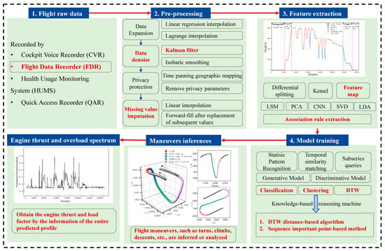
Figure 1.
Flow chart of engine thrust and load factor prediction method in this paper (The red item is the method applied in this paper).
The structure of this paper is organized as follows: Section 2 introduces the clustering and maneuver recognition methods involved in steps 3 and 4 of the workflow. In Section 3, the two proposed methods are employed to identify and categorize maneuvering actions of a specific aircraft based on acquired flight parameter data, completing the tasks outlined in step 5 of the workflow. Finally, Section 4 encompasses the prediction of thrust and load factors for the aircraft’s engine. In the Supplementary Materials, the current time series methods are validated and compared mathematically.
2. Real-Time Flight Maneuver Recognition (FMR) Method
Flight data is a typical high-dimensional, massive, and complex time series. Accordingly, two methods are proposed in this paper: a DTW distance-based algorithm and time series important point-based method for maneuver segmentation.
2.1. PLR–PIP Algorithm
First, the basic PLR–PIP algorithm is reviewed. Generally, the perceptually important point (PIP) in the time series is the point with the greatest distance value. Three distance measurements are commonly used: perpendicular distance (PD), vertical distance (VD), and Euclidean distance (ED) [26]. Figure 2 shows the three distances for a point in a certain sequence. For all three distances, the number of calculations required is the same. The graphs fitted by PD and VD are the same, but the value calculated using VD distance is the smallest. Therefore, this paper uses VD distance as the measurement value when analyzing flight parameters.
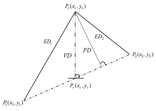
Figure 2.
Three methods to calculate distance: Perpendicular distance (PD), Vertical distance (VD), and Euclidean distance (ED).
Based on piecewise linear representation (PLR), a PLR–PIP method with a time series was proposed. The time series was represented by X = (x1, x1, …, xn) and the important series set the important points (IPs). The first point of the sequence is added to the set IPs. Then, each pair of adjacent points is taken as a sub-sequence and the PIP points are calculated and added to the set IPs. Adjacent PIP points form a new sub-sequence, which is linearly interpolated, and the root mean square error (RMSE) is calculated with respect to the original sequence. Sequences are extracted with RMSE values that do not meet the fitting error threshold condition. These steps are repeated until all sequences meet the threshold requirements . The algorithm flow is shown in Figure 3. According to this description of the improved strategies, PLR–PIP is given in Algorithm 1.
| Algorithm 1 PLP-PIP |
| Input: Row data, normal overload value sequence, threshold ΔPIP |
| 1: xb = dataMap.get(Pb); //get the value of begin point |
| 2: xe = dataMap.get(Pe); //get the value of begin point |
| 3: dist = 0; // Initial piecewise fitting error |
| 4: for i = 1→n do |
| 5: xi; = dataMap.get(i); //get the value of point i |
| 6: distsin[i] = cal(xb, Pb, xe, Pe, xi, Pi); //calculate the piecewise fitting error |
| 7: if distsin > ΔPIP then //If the piecewise fitting error ≥ ΔPIP |
| 8: continue //Add Perceptually Important Point |
| 9: else |
| 10: return (Pb, P1, P2, …, Pi, Pe); //get PIP set |
| 11: end if |
| 12: end for//Select the maneuver Sequences between PIP |
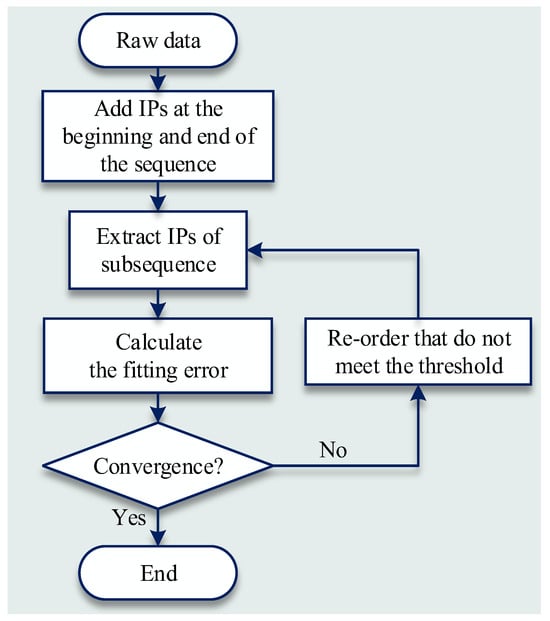
Figure 3.
Flow chart of PLR–PIP (IPs: important points).
Taking the altitude data of a certain flight as an example, the PLR–PIP calculation is performed with a fitting error threshold set to ΔPIP = 0.0001. The calculation process is demonstrated in Figure 4, where the dashed line represents the original sequence, the red dots represent PIP points, and the straight line represents the shape described using PIP. As the number of PIP increases, ΔPIP gradually decreases, and the data compression efficiency decreases as well. Therefore, the threshold ΔPIP needs to be set according to the actual situation.
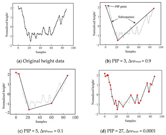
Figure 4.
The results by PLR–PIP, where the red dots represent PIP points.
2.2. Algorithm 2—Proposed DTW Distance-Based Algorithm
The flight maneuvers are connected through level flight, which has a relatively stable load factor of around 1 and stable parameters (roll angle, pitch angle, and altitude). Therefore, maneuvers can be divided based on the normal load factor of 1. Inspired by this, we propose a maneuver recognition method, called DTW distance-based algorithm (Table 1), with the following steps shown in Figure 5.

Table 1.
DTW distance-based algorithm.
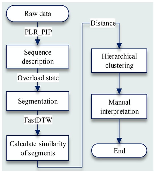
Figure 5.
Maneuver recognition algorithm based on Fast-DTW algorithm.
Two key steps, including the sequence description and improved hierarchical clustering algorithm, are described in detail.
2.2.1. Method and Principle by Sequence Re-Description
Since the normal load factor of an aircraft is approximately 1 during level flight, the starting and ending points of a maneuver can be identified by finding the segments with slight variations in the normal load factor and a mean value near 1. The trend is determined using the following rules. The actual gradient RPIP between two adjacent points (the ratio of the normal load factor difference between two points to the distance between two sample points) and the average normal load factor between two points are calculated in sequence. The threshold values of the slope and the average normal load factor are set as and , respectively. When the and , the segment between these two points is defined as a level flight maneuver. The results are shown in Figure 6, where the red curve represents the identified maneuver segments, and the black segments represent the level flight segments.
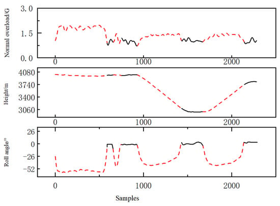
Figure 6.
The results of FMR (The black line represents level flight maneuvers, while the dotted line represents other maneuver characteristics.).
2.2.2. Improved Hierarchical Clustering Algorithm
If the similarity distance calculation is directly performed on various flight parameters of each segment, the difference in distance values calculated by different flight parameters will be significant. This will result in some parameters having a smaller impact weight on the similarity distance value of the segment. Therefore, before calculating the similarity distance, the flight parameters of each segment must be normalized. When calculating the similarity distances, the traditional DTW method has high computational complexity. The FastDTW method proposed in reference [10] greatly speeds up the calculation by constraining the space path at different levels. In this paper, the FastDTW library in Python is used to calculate the similarity distance values between different segments. The formula for calculating the similarity distance between two maneuver segments is shown in Equation (4), where a smaller value indicates a higher degree of similarity between the maneuver segments:
where is a parameter sequence of the maneuver segment and i is the ith flight parameter.
Similarity distance values can be calculated between both maneuver segments, thus a symmetric distance matrix with diagonal elements set to zero can be constructed to represent the differences between the segments. Let the sequence of all maneuver segments extracted from a certain takeoff and landing be denoted as ; the similarity distance matrix is
The hierarchical clustering analysis is performed for the similarity distance matrix due to its high precision and strong generality. However, after merging two classes each time, the hierarchical clustering algorithm must recalculate the distance matrix between classes, which burdens the computation when the number of classes is large. Therefore, an improved hierarchical clustering algorithm is proposed in this paper, and the algorithm process is shown in Figure 7.
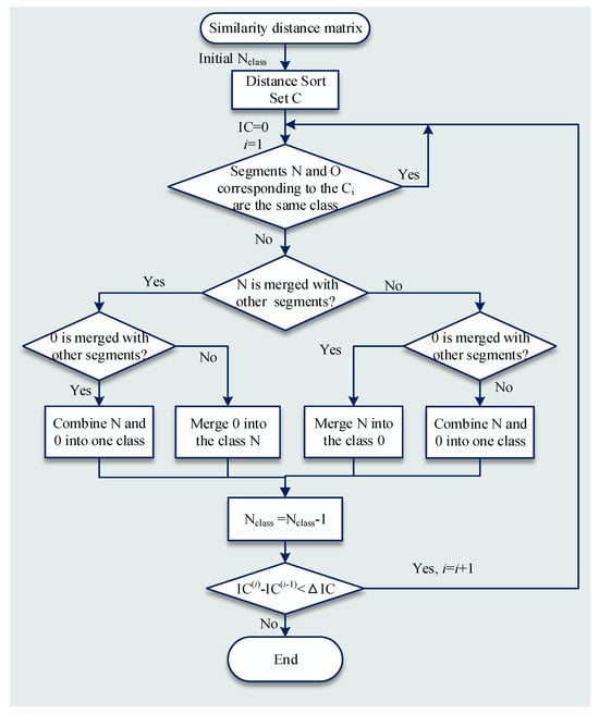
Figure 7.
Improved hierarchical clustering process.
2.2.3. Results of DTW Distance-Based Algorithm
Taking complete takeoff and landing data with 36,050 sampling points as an example, flight data, including normal load factor, altitude, pitch angle, roll angle, and heading angle curves, are shown in Figure 8; the horizontal axis represents the sampling point number. The data is inputted into the maneuver classification algorithm; its settings are shown in Table 2.
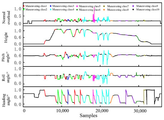
Figure 8.
MFR results based on the proposed DTW distance-based algorithm.

Table 2.
Parameter settings of the algorithm.
Due to the sensitivity of the foundational flight parameter data, normalization procedures are applied to the raw data using the following formula: DNorm = (D − Dmin)/(Dmax − Dmin). The MFR results based on the proposed DTW distance-based algorithm are shown in Figure 8; the straight flight segments formed during the middle partition process are defined as one class (i.e., class 10) without hierarchical clustering. Finally, 9 classes of maneuvers are formed, with a total of 22 maneuver segments. It can be seen that within a maneuver class, the trend and magnitude of the flight parameter data for each maneuver segment are similar, while significant differences exist between different maneuver classes.
To provide a more intuitive means of contrasting the differences among various maneuvers, an aircraft’s motion trajectory equations were established in a ground coordinate system. By examining the types of parameters contained in the measured data, it was determined that the aircraft’s trajectory could be recreated using the flight speed (v), track angle (Ψa), and altitude (H). The positional expression for any point on the trajectory is as follows:
Reproducing the trajectories for maneuver classes 1–9 based on the trajectory equations yields the results in Figure 9, the red dots represent turning points in maneuvers.
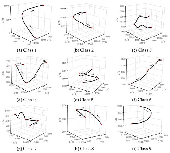
Figure 9.
Classification of maneuver with motion locus into 9 class based on the flight data, (a–i) shows 9 different maneuvering types that are manually defined, where the red dots represent turning points in maneuvers.
According to the above description of the improved strategies, the proposed DTW distance-based algorithm is given in Algorithm 2.
| Algorithm 2 Proposed DTW distance-based algorithm |
| Input: Row data, normal overload value sequence, threshold ΔPIP |
| 1: xb = dataMap.get(Pb); //get the value of begin point |
| 2: xe = dataMap.get(Pe); //get the value of begin point |
| 3: dist = 0; // Initial piecewise fitting error |
| 4: for i = 1→n do |
| 5: xi; = dataMap.get(i); //get the value of point i |
| 6: distsin[i] = cal(xb, Pb, xe, Pe, xi, Pi); //calculate the piecewise fitting error |
| 7: if distsin > ΔPIP then //If the piecewise fitting error ≥ ΔPIP |
| 8: continue //Add Perceptually Important Point |
| 9: else |
| 10: return (Pb, P1, P2, …, Pi, Pe); //get PIP set |
| 11: end if |
| 12: end for//Select the maneuver Sequences between PIP |
| 13: r0,0 = 0; ri,0 = r0,j = ∞; i ∈ [n], j ∈ [m] |
| 14: for j = 1, 2, …, m do //Sequence 1 |
| 15: for i = 1, 2, …, n do //Sequence 2 |
| 16: ri,j = δ(xi, yi) + min {ri−1,j−1, ri−1,j, ri,j−1} //Calculate Sequence similarity |
| 17: Hierarchical clustering |
| 18: end for |
| 19: end for |
| Output: Mancuver |
2.3. Algorithm 3—Proposed Sequence Important Point-Based Method
2.3.1. Method and Principle of Sequence Important Point
In flight dynamics, aircraft maneuvers are classified into three categories: vertical plane maneuvers, horizontal plane maneuvers, and spatial maneuvers. This paper proposes a maneuver classification algorithm based on the time series of significant points, using the trend states of trajectories projected onto the horizontal and vertical planes. The specific steps are as follows:
Step 1. Divide the flight parameters into multiple segment sequences with fixed lengths, and the trajectory of each sequence is projected onto the horizontal plane.
Step 2. Using certain merging rules, the PLR–PIP algorithm is used to segment the trajectory projection, identify the sequence trend, and merge adjacent trend sequences with the same state.
Step 3. Project the merged trend sequences onto the vertical plane; the PLR–PIP algorithm is used to segment the trajectory projection, identify the sequence trend, and subdivide the trend sequences by subdivision rules.
Step 4. Superimpose the trend states of the two plane projections to obtain the basic aircraft maneuvers, shown in Figure 10.
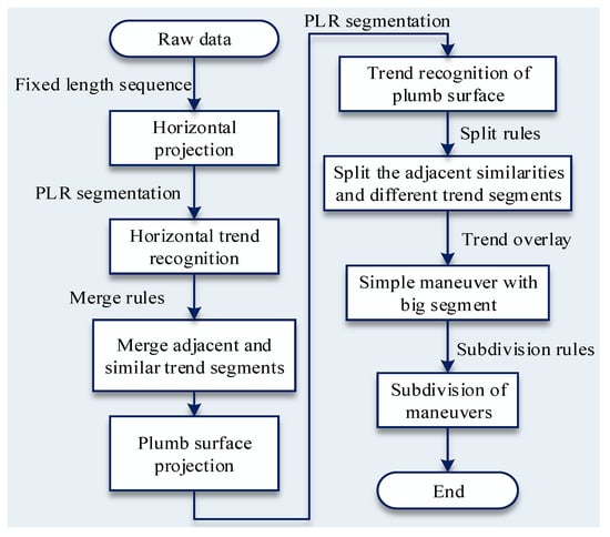
Figure 10.
Flow chart of proposed sequence important point-based method.
According to this description of the improved strategies, the proposed sequence important point-based method is provided in Algorithm 3. The trend recognition and subdivision/merge rules are important and described in the following section.
| Algorithm 3 Proposed Perceptually important point-based method |
| Input: Row data, n, dPIP, kPIP |
| 1: Divide the raw data into sequences of length n |
| 2: Perform PLR-PIP segmentation on the horizontal projection of the sequences |
| 3: for i = 1→m do |
| 4: d = |(y1 + (y2 − y1)[(xi − x1)/(x2 − x1)] − yi)|; //get the value of VD |
| 5: D = (d1, d2, …, dm)//get the distance set |
| 6: if di ≤ dPIP then |
| 7: Straight sequence |
| 8: else |
| 9: Bending sequence |
| 10: end if |
| 11: end for |
| 12: Perform PLR-PIP segmentation on the vertical projection of the sequences |
| 13: for j = 1 → ω do |
| 14: Calculate the slope of adjacent, PIP points |
| 15: D = (k1, k2, …, kω)//get the slopes set |
| 16: if kj ≤ −kPIP then |
| 17: Descend sequence |
| 18: else if −kPIP < kj < kPIP then |
| 19: Level sequence |
| 20: else |
| 21: Ascend sequence |
| 22: end if |
| 23: end for |
| 24: Combine into maneuver |
| Output: Maneuver |
2.3.2. Trend Recognition and Subdivision/Merge Rules
Regarding the projection onto the horizontal plane, the focus is on changes in the flight direction, which can be described using straight or curved lines with the trajectory coordinates. Meanwhile, for the vertical plane, the focus should be on the changes in altitude, which can be described using horizontal, upward, and downward directions.
(1) Recognition rules for vertical projection. Two methods are used for projection onto the vertical plane: using the transformation or the altitude time series. Taking the somersault maneuver height trajectory of a certain flight as an example, the difference between the two projection methods is compared in Figure 11; the black curve represents the maneuver trajectory, the arrow indicates the direction of flight and the red dots represent the start and end points of the somersault and the segmentation points of the upward and downward sections. Both methods describe the altitude trend of the maneuver, but under the transformation projection, the upward and downward sections of the somersault show a positive upward trend, which can lead to confusion in trend recognition. In contrast, the upward and downward sections of the somersault align exactly with those of the projection when using the time series of altitude for projection. Therefore, using the altitude time series for projection is more reasonable.

Figure 11.
Projections of a somersault motion on the vertical plane, where the red dashed arrow indicates the direction of flight.
(2) Recognition rules for horizontal projection. First the original flight parameter data sequence is divided into multiple segments of equal length n. Let a sequence contain n sequence points, and denote the horizontal coordinate of the trajectory of the sequence in a new spatial coordinate X = (x1, x2, …, xn), Y = (y1, y2, …, yn), and Z = (z1, z2, …, zn). On the projection of the sequence onto the horizontal plane, PLR–PIP is performed to obtain a set of sub-sequence segments (PLR1 and IPs1 sets) where the PIP point sequence is denoted by the x-coordinate and y-coordinate . Another PIP point is selected from each sub-sequence segment, and the VD distance of the individual sub-sequence is calculated, with the distance set denoted as . A distance threshold is defined as , where a sub-sequence is classified as a straight primitive if , and as a curved primitive if . Upon projecting the sequence onto the height coordinate system, PLR–PIP segmentation is performed to obtain a set of sub-sequence segments. Note ) as the gradient set between each PIP and as a gradient threshold. When , the interval is marked as a descent element; when , the interval is marked as a horizontal element; when , the interval is marked as an ascent element.
(3) Segments merge. When defining the initial value of n, a basic maneuver segment may be divided into multiple adjacent trend sequences, which must be merged into one trend sequence. However, the merged sequence may have a change in overall trend; for example, two straight-line primitives may merge into a curved primitive. Therefore, after merging, the trend fitting of the sequence must be re-recognized. This process of repeating sequence state recognition and merging continues until there are no adjacent trend sequences and the trend sequence merging is completed. As shown in Figure 12, fifteen straight-line primitives are merged into one curved primitive sequence.
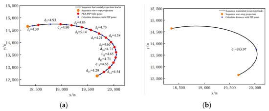
Figure 12.
Trend merging. (a) before merging; (b) after merging.
When projecting horizontal trend sequences onto the vertical plane for trend recognition, there may be multiple segments within a single sequence, such as an upward segment followed by a horizontal segment. In this case, PIP points are used to examine the trend of the sequence, and if the trend is inconsistent, the sequence is subdivided at the point of trend change using PIP points to form separate segments, and the trend of each segment is recalculated. As shown in Figure 13, a sequence is subdivided into four sequences: downward, horizontal, upward, and horizontal.
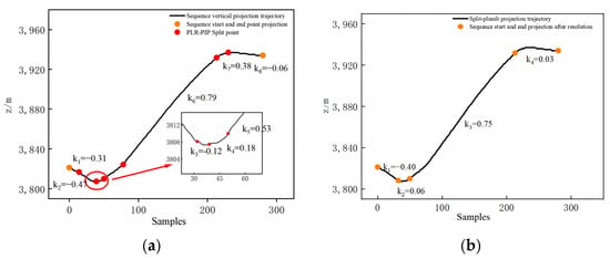
Figure 13.
Trend subdivision (a) before subdivision (b) after subdivision.
2.3.3. Results of Sequence Important Point-Based Method
Taking complete takeoff and landing data as an example, the trajectory is projected onto the horizontal plane. The trajectory data is divided into multiple sequences of length n = 24, and dpip = 5 and Δpip = 0.001. The resulting partition of the aircraft flight trajectory on the horizontal plane can be obtained, as shown in Figure 14.
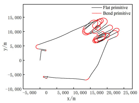
Figure 14.
Trend identification results on a horizontal plane.
Eighty-six horizontal trend segments are projected onto the vertical plane, and trend recognition is performed. Using ΔPIP = 0.01, the PIP points of the vertical trend sequence are extracted, and the slope between each PIP point is calculated. The rules for superimposing states are shown in Table 3. This paper utilizes criteria based on the changes in flight parameters, such as velocity, height, pitch angle, and roll angle. For detailed division criteria, refer to Table 4. Finally, 14 classes of refined maneuver states are formed. The results of the simple maneuvers and task segment division are shown in Figure 15, where the altitude data have been normalized.

Table 3.
Rules for superimposing states.

Table 4.
State subdivision criteria.
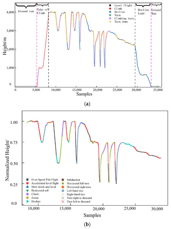
Figure 15.
Segment classification: (a) Simple maneuver recognition, (b) Subdivision of simple maneuvers.
3. Comparison of the Two Proposed Maneuver Classification Algorithms
By comparing the classification concept and results of the two algorithms, the following three differences were obtained:
- (1)
- Acquisition of maneuver segments
Algorithm 2 acquires maneuver segments by analyzing the feedback of flight parameter data during intense aircraft maneuvering and obtaining corresponding maneuver segments based on the highlighted segments of the normal load factor. This method can obtain most action segments during intense maneuvering. However, for some moments when the aircraft performs smooth maneuvering with small changes in flight parameter data, Algorithm 2 may not accurately extract the maneuver segments, resulting in recognition errors. For example, between sampling points 5820 and 8250, when the aircraft is performing a slow climb, Algorithm 2 fails to identify it as a maneuver segment and instead categorizes it as a level flight segment. Algorithm 3 segments the trajectory by trend recognition of the horizontal and vertical projections with a fixed step length and identifies the trend change points to ultimately obtain maneuver segments. In the segmentation process, no data segments are skipped or discarded, so there is no situation where a segment is not recognized.
- (2)
- Hierarchical maneuver segments
The maneuver segments extracted by Algorithm 2 are continuous and correspond to intense changes in the normal load factor or high average normal load factors. Algorithm 2 can accurately recognize and segment complex combination maneuvers, such as a half-roll and a somersault. It can also recognize specific unnamed maneuvers. For example, Algorithm 2 segments the maneuver between sampling points 20,380 and 21,360 as a complete maneuver segment (maneuver class 4), which is identified through manual recognition as a combination of climbing, right turn climbing, right turn descent, dive, left turn climbing, and climbing tactical maneuvers. Algorithm 3 identifies basic maneuver actions based on the horizontal and vertical projection trend, and complex combination maneuvers require additional merge rules to be recognized. For example, Algorithm 3 segments the maneuver between sampling points 20,050 and 21,518 into six maneuver actions: climb (21,260–21,555), right turn ascent (21,556–21,749), right turn descent (21,750–21,855), dive (21,856–22,070), left turn ascent (22,071–22,316), and climb (22,317–22,660). In Figure 16, the left side shows the 3D display of the trajectory, the upper right corner shows the vertical projection of the trajectory, and the lower right corner shows the horizontal projection of the trajectory.
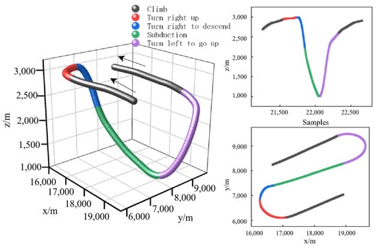
Figure 16.
Motion decomposition for maneuver class 4.
Both algorithms effectively identify the actions in this interval, but their emphasis on segmentation hierarchy differs. The results of Algorithm 2 are a combination of the results of Algorithm 3, and similar combination maneuvers can be classified into one class without the need for additional rules. Algorithm 3 provides a deeper and more detailed segmentation of the maneuver segments identified by Algorithm 2. The four sampling point intervals corresponding to the maneuver class 4 identified by Algorithm 2 are also reflected in the results of Algorithm 3. Additionally, Algorithm 3 considers the differences in turning direction between the maneuver actions of maneuver class 4.
- (3)
- Normalization of maneuver segments
After Algorithm 2 forms the maneuver classes, an issue arises with providing standardized descriptions, as it remains unclear which specific actions each maneuver class represents. Manual recognition is often required for complex combination actions, such as maneuver class 4, but Algorithm 2 greatly reduces the workload of manual recognition and the disadvantages of obtaining standard action templates. After Algorithm 3 forms the maneuver segments, the segment is the basic action type. Although criteria must be manually added to obtain complex combination maneuvers, this paper focuses on the load history of the engine under different states. Therefore, the engine’s state division should be as detailed as possible, and the kinematic equation of the engine’s center of mass is calculated in a small time segment. As such, the fewer changes in the maneuver state during the divided small-time segment, the better. As a result, there is no need to add overly complex action merging rules. According to the state subdivision criteria proposed in Table 4, it is sufficient to standardize the description of most flight states. Considering these factors, Algorithm 3 is used for maneuver action division in the subsequent analysis of this paper.
Algorithm 2 allows fine-tuning by adjusting parameters to alter clustering outcomes. However, as pilot training shifts from “routine” to more “combat-like” scenarios with unpredictable maneuvers, clustering becomes prone to misjudgment, leading to arbitrary results, such as incomplete or mixed maneuvers. In contrast, Algorithm 3 offers better recognition accuracy, while Algorithm 2 is operationally complex and more costly.
4. Prediction of Engine Thrust and Load Factor
4.1. Flight Load Calculation of Aircraft Engine
Drawing upon the principles of finite element analysis, this method involves a systematic extraction of incremental trajectory segments within the provided comprehensive flight segment. Subsequently, these diminutive trajectory segments are the focal point for the meticulous computation of aircraft engine flight loads. The procedural framework is delineated as follows:
Step 1 Aircraft Model Specification:
Initial proceedings necessitate the determination of essential design parameters for the aircraft model, encompassing attributes such as the empty weight, the relationship between lift coefficient and angle of attack, zero-lift drag coefficient, lift-induced drag factor, wing area, engine installation angle, and analogous specifications. Employing the least squares method principle, a fitted curve function, predicated on the aircraft’s polar curve and informed by design parameters, is deduced. This mathematical representation facilitates the derivation of lift and drag coefficients across a spectrum of variables, including angle of attack, Mach number, and altitude.
Step 2 Acquisition of Trajectory Data:
Subsequently, requisite data for the computation of aircraft engine flight loads are acquired from measured flight parameters. These encompass fuel weight, airspeed, pitch angle, roll angle, angle of attack, flight path angle, sideslip angle, and other pertinent variables. Retrieval of pertinent flight parameter data is limited to defined temporal intervals.
Step 3 Calculation of Aircraft Drag:
The flight parameter data forms the basis for calculating the aircraft’s lift-to-drag ratio. The computed value is subsequently utilized in Equation (7) to determine the aircraft’s drag within the confines of the current incremental segment.
where Qi represents the current minute segment of drag, ρv2/2 is dynamic pressure, S represents the wing area, CX is the aircraft’s drag coefficient, CX0 is the zero-lift drag coefficient, A is the lift-induced drag factor, ΔCXh is the drag coefficient’s altitude correction value, and CYi is the lift coefficient for the current minute segment.
Step 4 Calculate engine thrust
We ascertain the requisite thrust for the aircraft by employing the differential equations governing the aircraft’s center of mass dynamics in the context of the trajectory coordinate system with the contemporaneous flight parameter data. Subsequently, the actual thrust delivered by the engines is determined in accordance with the thrust efficiency conversion ratio.
where Pi represents the available thrust for the current minor segment of the aircraft, mi is the mass of the aircraft in the current minor segment; vi is the flight vector velocity for the current minor segment of the aircraft; Ri is the engine thrust; η is the thrust efficiency conversion ratio; φp is the angle between the engine thrust vector and the aircraft’s axis Oxb at specific times; αi is the angle between the projection of airflow axis Oxa on the aircraft’s symmetry plane and the body axis Oxb; βi is the angle between the airflow axis Oxa and the aircraft’s symmetry plane; θi is the angle between the trajectory axis Oxk and the horizontal plane that is positive upwards relative to the terrain.
The ground coordinate system is a fixed system attached to the Earth’s surface. The origin, O, can be set at any location on the ground, typically chosen at the point of aircraft takeoff. The directions of the axes are generally determined using the right-hand rule.
The range for the parameter η typically falls between 90% and 95%. In this study, we opted for a η value of 90%. By selecting a lower efficiency conversion ratio, we intentionally calculate aircraft thrust requirements that are higher than actual values, anticipating a more significant load than reality. This approach ensures that the calculated results lean toward safety.
Step 5 Calculate the lift and side forces
The next step involves the computation of aircraft lift and lateral force by integrating the current flight parameter data with the previously determined aircraft drag values within the current trajectory segment as follows:
where Yi represents the lift along the Oya direction; Zi represents the lateral force along the Oza direction; γsi represents the angle between the airflow Oya-axis and the flight path Oyk, known as the roll angle; the Ψai track angle, also referred to as the heading angle, is the angle between the projection of the flight path Oxk-axis on the horizontal plane and the ground Oxg-axis, with the convention that rightward is positive.
Step 6 Calculation of load factor
During flight, an aircraft constantly alters its speed, altitude, and heading. The faster these three parameters change, the better the aircraft’s maneuverability. The maneuverability can be characterized by the aircraft’s tangential and normal accelerations, where a larger acceleration corresponds to greater external forces acting on the aircraft. The load factor on the aircraft, defined as the ratio of the sum of all forces on the aircraft, excluding gravity, to the aircraft’s weight, is a critical parameter. The aircraft’s load factor is interconnected with the engine load factor. The load factor is a vector, and its projection on the trajectory coordinate axes is as follows:
here, nxi, nyi, nzi are the engine load factor in the current path coordinate frame, respectively.
Step 7 Check the calculation results
After completing one calculation, check if there are any remaining informational segments. Continue to extract small informational segments and follow steps 2 to 6 to compute engine load information. Ultimately, this process yields engine load information for the entire time interval.
4.2. Engine Flight Load and Thrust Prediction
During the aircraft’s flight load calculations, derivations are conducted using flight parameter information at various instances. When making predictions, only the type of maneuver action is known, and detailed flight parameter data throughout the maneuver action sequence is lacking. Therefore, it is necessary to investigate the parameters governing maneuver actions, establish parameter equations, and provide a parameterized description of the motion.
Step 1 Weight of aircraft
When considering the pattern of aircraft weight variation, the first step involves determining whether the aircraft performs actions such as missile launches or equipment drops during the flight. By excluding such actions, the primary cause of aircraft weight variation becomes fuel consumption. Subsequently, using empirical data, the relationship between the rate of fuel consumption and maneuver actions is calculated. This yields a time-based profile of aircraft weight variation characterized by a nearly steady pattern.
Based on multiple flight profiles, the aircraft’s weight is calculated as 2700 kg, with an initial fuel quantity of 1700 L, and the fuel consumption rates during various time intervals are detailed in Table 5. Lastly, through the division of missions and task actions, the aircraft’s weight at each moment can be determined.

Table 5.
State subdivision criteria.
Step 2 Prediction of pitch angle
When the aircraft performs maneuver actions, there are three types of pitch angle variations: (1) starting from an initial value, maintaining a fixed rate of change until reaching an extreme value, and returning to the initial value at the end of the action; (2) starting from 0°, changing at a fixed rate to reach an extreme value, and maintaining that angle until the end of the action; (3) starting from 0°, changing at a fixed rate to reach an extreme value, and then returning to 0° at a fixed rate (Figure 17).
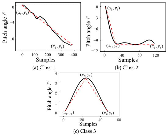
Figure 17.
Classification of pitch angle, where the red dashed line represents the results of linear fitting. (a–c) represent parameter fitting results for three different scenarios, respectively.
Parameter fitting can be achieved by constructing various linear equations. The positional information required during the linear fitting process was acquired during the statistical analysis. This information includes the action’s starting point in time, the time at which the pitch angle reaches its extreme value, the time when the action ends, the initial pitch angle at the start of the action, and the pitch angle at the extreme point of the action. In Figure 17, the black curve represents the observed pitch angle change of the aircraft during the maneuver, and the red curve (dashed line) represents the linear fitting result.
Step 3 Prediction of roll angle
The variation in the aircraft’s roll angle typically corresponds to turning maneuvers. The aircraft’s roll angle begins at 0° and increases at a specified rate to reach the prescribed roll angle. Depending on the specific maneuver, it maintains the current roll angle for a certain period. It then returns the roll angle to zero at a fixed rate, marking the end of the action, as illustrated in Figure 18. In most cases, the rate of change in reaching the extreme value of the roll angle and returning from the extreme value to zero is the same. Therefore, similar to the pitch angle, it can be fitted using three linear equations where x1 corresponds to the start time of the action, x2 corresponds to the time of the roll angle reaching its extreme value, x4 corresponds to the end time of the action, y1 corresponds to the initial roll angle at the start of the action, and y2 corresponds to the roll angle at the extreme point of the action. In Figure 18, the black curve represents the observed changes in the aircraft’s roll angle during maneuvers, and the red curve (dashed line) represents the linear fitting result.
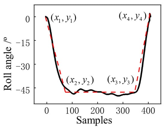
Figure 18.
Roll angle change history, where the red dashed line represents the results of linear fitting.
Step 4 Altitude and Atmospheric Density
The aircraft’s flight altitude and atmospheric density are crucial parameters in calculating the aircraft’s lift-to-drag ratio. Flight altitude is a function of time based on flight speed and pitch angle. By integrating the previously obtained functions for speed and pitch angle and considering the initial altitude, we can determine the altitude at each moment. The calculation relationship is expressed as Equation (11).
where represents the flight altitude at time t1, H0 is the initial altitude, v is the flight speed, and ϑ is the pitch angle.
As shown in Figure 19, the black curve represents the observed velocity, pitch angle, and altitude profiles during the maneuver action. The red curve (dashed line) represents the results of linear fitting for the velocity and pitch angle profiles and the altitude profile after integration.

Figure 19.
Parameter fitting results (The red dashed line represents the results of fitting). (a) represents the Velocity fitting result, (b) represents the Pitch angle fitting result, and (c) represents the Height fitting result.
An inverse relationship exists between altitude and atmospheric density, as indicated by the relationship in Equation (12). After obtaining information on the altitude variation profile, atmospheric density ρ at each height H can be calculated using the following formula:
By solving the parameter histories of each maneuver, the flight trajectory information of the entire predicted profile, and the engine altitude change under the typical profile can be obtained, where the altitude coordinates have been normalized (Figure 20).
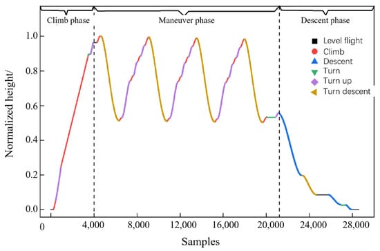
Figure 20.
Altitude changes of the predicted profile.
To obtain the engine thrust and load factor of the typical profile, the aircraft performance information and height, pitch angle, roll angle, etc., obtained from steps 1 and 2, are combined with the thrust and load factor calculation method in Section 4.1. The predicted engine thrust, engine normal load factor, and the tangential load factor of the typical profile can be obtained, as shown in Figure 21, Figure 22 and Figure 23, where each parameter on the vertical axis has been normalized.
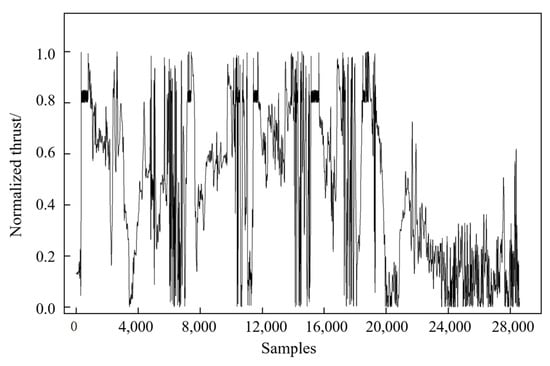
Figure 21.
Predicted thrust for aero-engine.
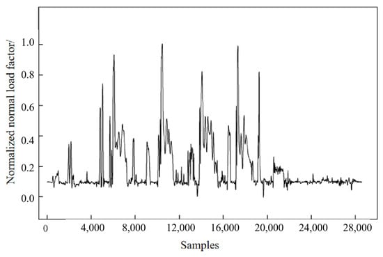
Figure 22.
Predicted normal load factor for aero-engine.
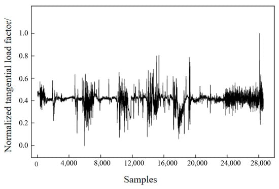
Figure 23.
Predicted tangential load factor for aero-engine.
5. Conclusions
In this paper, we present two novel maneuver recognition algorithms based on the data characteristics of specific flight test data. These methods include the DTW distance-based algorithm (Algorithm 2) and the sequence important point-based algorithm (Algorithm 3). Using a given flight data model as a case study, we derived and computed the thrust and load factors for various maneuvering conditions. The conclusions are summarized as follows:
(1) Algorithm 2 obtains maneuver segments by analyzing the feedback from flight parameter data in different aircraft maneuvers. This method can capture more segments during high-intensity maneuvers and accurately identify and categorize complex composite maneuvers, such as half-rolls, somersaults, and other specific maneuvers. For instance, Algorithm 2 classifies the maneuver as a complete maneuver segment (maneuver class 4), which, upon manual inspection, represents a tactical composite maneuver that sequentially includes the continuous sequence of climb, right turn-climb, right turn-descent, dive, left turn-climb, climb. However, for smoother maneuvers where the rate of change in flight parameter data is small, it may be challenging to precisely extract maneuver segments, resulting in a degree of recognition error.
(2) Algorithm 3 identifies maneuver segments by progressively recognizing trends in the horizontal and vertical plane projections of the trajectory. It uses a fixed step size to segment areas with trend changes (clusters) and subsequently extract maneuvers. This segmentation process does not skip or discard data segments, improving recognition capability. However, Algorithm 3 primarily identifies fundamental maneuver actions, and recognizing complex composite maneuvers requires the incorporation of specific merging rules, increasing the recognition efficiency and complexity, while manual judgment may also be necessary. Nonetheless, to identify and predict engine load histories under different aircraft states in this particular case, there is no need to identify numerous maneuver states. Hence, Algorithm 3 is more suitable for the scenario in this paper.
(3) In this study, unconventional techniques in time series data analysis are employed, primarily involving the utilization of the perceptually important points (PIP) procedure to encode and structure individual time series data from each station. This innovative approach effectively reduces dimensionality while preserving the underlying pattern structure; subsequently, a set of rules is applied for dataset classification.
(4) The flight mission profile comprises various mission-specific actions, and differing actions lead to variations in the acquired aircraft flight data. Consequently, the derived load histories are also distinct. Before the design phase, aircraft operating departments have made preliminary determinations regarding the aircraft’s flight missions. Therefore, it is possible to derive different aircraft design loads by analyzing mission-specific requirements.
(5) From the load factor data associated with the aforementioned maneuvers, it is evident that the engine load factor is intricately linked to the aircraft’s state. Variations in aircraft characteristics and flight mission conditions result in different engine profiles. Thus, the initial proposal in this study, focusing on the investigation of engine thrust and load factors based on mission requirements, is deemed imperative.
In summary, it is possible to derive the thrust characteristics of a new aircraft engine by analyzing the flight mission profiles, obtaining flight test data or empirical flight parameters, and subsequently solving the fundamental aircraft flight dynamics equations. Following this, the design methodology for the new aircraft engine can be determined using statistical methods based on the mission cycles.
Supplementary Materials
The following supporting information can be downloaded at: https://www.mdpi.com/article/10.3390/aerospace10110961/s1, Figure S1: 1-NN accuracy of proposed different alignment measures on UCR datasets. Figure S2: 1-NN error analysis of proposed different alignment measures compared with FastDTW. Table S1: Comparison of accuracy and time. Table S2: Comparison of accuracy and time. Reference [27] are cited in the Supplementary Materials.
Author Contributions
Conceptualization, M.Z. and Z.Y.; methodology, M.Z. and Z.Y.; software, S.X. and J.T.; validation, Y.H. and J.T.; formal analysis, S.X., Y.H. and J.T.; writing—original draft preparation, M.Z. and J.T.; writing—review and editing, S.X., Y.H. and Z.Y.; supervision, Z.Y.; funding acquisition, M.Z. All authors have read and agreed to the published version of the manuscript.
Funding
This work was supported by Guangdong Basic and Applied Basic Research Foundation (Grant 2022A1515110636), the National Natural Science Foundation of China (Grant No. 12302156), the Natural Science Basic Research Plan in Shaanxi Province of China (No. 2023-JC-QN-0012), and the National Science Technology Major Project (J2019-IV-0017-0085).
Data Availability Statement
Data available on request due to restrictions eg privacy or ethical.
Conflicts of Interest
The authors declare no conflict of interest. The funders had no role in the design of the study; in the collection, analyses, or interpretation of data; in the writing of the manuscript, or in the decision to publish the results.
Abbreviation
| CDTW | Context-based dynamic time warping |
| CNN | Convolutional Neural Network |
| CTW | Context-Tree Weighting |
| DBSCAN | Density-based spatial clustering of applications with noise |
| DTW | Dynamic time warping |
| ED | Euclidean distance |
| FAA | Federal Aviation Administration |
| FDR | Flight data recorder |
| FMR | Flight Maneuver Recognition |
| IC | Inconsistency coefficient |
| IPs | Important points |
| LDA | Latent Dirichlet Allocation |
| LSM | Logistic Sigmoid Model |
| PCA | Principal Component Analysis |
| PD | Perpendicular distance |
| PIP | Perceptually important point |
| PLR | Piecewise linear representation |
| RMSE | Root mean square error |
| SVD | Singular Value Decomposition |
| VD | Vertical distance |
| 1-NN | 1-nearest neighbors |
References
- Duncan, J.S. Pilot’s Handbook of Aeronautical Knowledge; Airman Testing Standards Branch, Federal Aviation Administration, United States Department of Transportation: Oklahoma City, OK, USA, 2016.
- Yin, D. Design of Flight Training Evaluation System Based on Flight Parameters Data. In Proceedings of the 2022 IEEE 8th International Conference on Computer and Communications (ICCC), Chengdu, China, 9–12 December 2022; IEEE: Piscataway, NJ, USA. [Google Scholar]
- Mangortey, E.; Mangortey, E.; Monteiro, D.; Ackley, J.; Gao, Z.; Puranik, T.G.; Kirby, M.; Pinon-Fischer, O.J.; Mavris, D.N.; Jimenez, H.; et al. Application of machine learning techniques to parameter selection for flight risk identification. In Proceedings of the AIAA Scitech 2020 Forum, Orlando, FL, USA, 6–10 January 2020. [Google Scholar]
- Singh, K.L.; Venkatasubramanyam, D. Techniques to Generate and Optimize the Load Spectra for an Aircraft. Int. J. Mech. Mater. Des. 2010, 6, 63–72. [Google Scholar] [CrossRef]
- Lu, Q.; Sun, Z.; Xu, C.; Zhao, S.; Song, Y. A new compilation method of general standard test load spectrum for aircraft engine. Int. J. Turbo Jet-Engines 2022, 39, 13–23. [Google Scholar] [CrossRef]
- Niu, X.; Lu, Q.; Sun, Z.; Song, Y. A novel compilation method of comprehensive mission spectrum of aero-engine maneuvering load based on use-related mission segment. Chin. J. Aeronaut. 2023, 36, 161–170. [Google Scholar] [CrossRef]
- Lu, J.; Pan, L.; Deng, J.; Chai, H.; Ren, Z.; Shi, Y. Deep learning for flight maneuver recognition: A survey. Electron. Res. Arch. 2023, 31, 75–102. [Google Scholar] [CrossRef]
- Gavrilovski, A.; Jimenez, H.; Mavris, D.N.; Rao, A.H.; Shin, S.; Hwang, I.; Marais, K. Challenges and opportunities in flight data mining: A review of the state of the art. In Proceedings of the AIAA Infotech@ Aerospace, San Diego, CA, USA, 4–8 January 2016; p. 0923. [Google Scholar]
- Wang, B.; Liu, D.; Wang, W.; Peng, X. A hybrid approach for UAV flight data estimation and prediction based on flight mode recognition. Microelectron. Reliab. 2018, 84, 253–262. [Google Scholar] [CrossRef]
- Salvador, S.; Chan, P. Toward accurate dynamic time warping in linear time and space. Intell. Data Anal. 2007, 11, 561–580. [Google Scholar] [CrossRef]
- Ni, S.H.; Shi, Z.K.; Xie, C.; Wang, Y.H. Establishment of avion inflight maneuver action recognizing knowledge base. Comput. Simul. 2005, 22, 23–26. [Google Scholar]
- Wang, Y.; Dong, J.; Liu, X.; Zhang, L. Identification and standardization of maneuvers based upon operational flight data. Chin. J. Aeronaut. 2015, 28, 133–140. [Google Scholar] [CrossRef]
- Sharif, M.; Alesheikh, A.A. Context-awareness in similarity measures and pattern discoveries of trajectories: A context-based dynamic time warping method. GISci. Remote Sens. 2017, 54, 426–452. [Google Scholar] [CrossRef]
- Meng, G.; Chen, Z.; Luo, Y. Maneuvering action identify method based on dynamic Bayesian network. J. Syst. Simul. 2017, 29, 140–145. [Google Scholar]
- Lu, J.; Chai, H.; Jia, R. A general framework for flight maneuvers automatic recognition. Mathematics 2022, 10, 1196. [Google Scholar] [CrossRef]
- Miyamoto, S.; Ichihashi, H.; Honda, K.; Ichihashi, H. Algorithms for Fuzzy Clustering; Springer: Berlin/Heidelberg, Germany, 2008; Volume 10. [Google Scholar]
- Qu, J.; Lv, M.; Yang, Y.; Tang, Y. Flight motion recognition method based on multivariate phase space reconstruction and approximate entropy. In Proceedings of the 2021 40th Chinese Control Conference (CCC), Shanghai, China, 26–28 July 2021; IEEE: Piscataway, NJ, USA, 2021. [Google Scholar]
- Zhou, Y.; Lu, Z. An enhanced Kriging surrogate modeling technique for high-dimensional problems. Mech. Syst. Signal Process. 2020, 140, 106687. [Google Scholar] [CrossRef]
- Pathirage, C.S.N.; Li, J.; Li, L.; Hao, H.; Liu, W.; Ni, P. Structural damage identification based on autoencoder neural networks and deep learning. Eng. Struct. 2018, 172, 13–28. [Google Scholar] [CrossRef]
- Meng, G.; Zhang, H.; Piao, H.; Liang, X.; Zhou, M. Recognition of fighter maneuver in automatic flight training evaluation. J. Beijing Univ. Aeronaut. Astronaut. 2020, 46, 1267–1274. [Google Scholar]
- Wei, Z.; Ding, D.; Zhou, H.; Zhang, Z.; Xie, L.; Wang, L. A flight maneuver recognition method based on multi-strategy affine canonical time warping. Appl. Soft Comput. 2020, 95, 106527. [Google Scholar] [CrossRef]
- Barratt, S.T.; Kochenderfer, M.J.; Boyd, S.P. Learning probabilistic trajectory models of aircraft in terminal airspace from position data. IEEE Trans. Intell. Transp. Syst. 2018, 20, 3536–3545. [Google Scholar] [CrossRef]
- Li, L.; Hansman, R.J.; Palacios, R.; Welsch, R. Anomaly detection via a Gaussian Mixture Model for flight operation and safety monitoring. Transp. Res. Part C Emerg. Technol. 2016, 64, 45–57. [Google Scholar] [CrossRef]
- Hong, S.; Lee, K. Trajectory prediction for vectored area navigation arrivals. J. Aerosp. Inf. Syst. 2015, 12, 490–502. [Google Scholar] [CrossRef]
- Li, L.; Das, S.; Hansman, R.J.; Palacios, R.; Srivastava, A.N. Analysis of flight data using clustering techniques for detecting abnormal operations. J. Aerosp. Inf. Syst. 2015, 12, 587–598. [Google Scholar] [CrossRef]
- Chung, F.L.K.; Fu, T.C.; Luk, W.P.R.; Ng, V.T.Y. Flexible time series pattern matching based on perceptually important points. In Proceedings of the Workshop on Learning from Temporal and Spatial Data in International Joint Conference on Artificial Intelligence, Seattle, WA, USA, 1 January 2001. [Google Scholar]
- Cover, T.; Hart, P. Nearest neighbor pattern classification. IEEE Trans. Inf. Theory 1967, 13, 21–27. [Google Scholar] [CrossRef]
Disclaimer/Publisher’s Note: The statements, opinions and data contained in all publications are solely those of the individual author(s) and contributor(s) and not of MDPI and/or the editor(s). MDPI and/or the editor(s) disclaim responsibility for any injury to people or property resulting from any ideas, methods, instructions or products referred to in the content. |
© 2023 by the authors. Licensee MDPI, Basel, Switzerland. This article is an open access article distributed under the terms and conditions of the Creative Commons Attribution (CC BY) license (https://creativecommons.org/licenses/by/4.0/).