Three-Dimensional Path-Following Control Method for Flying–Walking Power Line Inspection Robot Based on Improved Line of Sight

Abstract

The Flying–Walking Power Line Inspection Robot (FPLIR) faces challenges in maintaining stability and reliability when operating in harsh transmission line environments with complex conditions. The robot often switches modes frequently to land accurately on the line, resulting in increasing following errors and premature or delayed switching caused by reference path switching. To address these issues, a path-following control method based on improved line of sight (LOS) is proposed. The method features an adaptive acceptance circle strategy that adjusts the radius of the acceptance circle of the path point based on the angle of the path segment and the flight speed at the time of switching, improving path-following accuracy during reference trajectory switching. Also, an adaptive heading control with vertical distance feedback is designed to prioritize different path-following methods in real time based on variations in vertical distance, achieving rapid convergence along the following path. The state feedback following control law, based on the improved LOS, achieves the stable following of the reference path, which was validated by simulations. The simulation results show that the improved LOS reduces the convergence time by 0.8 s under controllable error conditions for path angles of θ ∈ (0, π⁄2). For path angles of θ ∈ (π⁄2, π), the following error is reduced by 0.3 m, and the convergence time is reduced by 0.4 s. These results validate the feasibility and effectiveness of the proposed method. This method demonstrates advantages over the traditional LOS in terms of following accuracy and convergence speed, providing theoretical references for future 3D path following for path-following robots and aerial vehicles.

1. Introduction

The power industry plays a vital role in socioeconomic development. However, because of factors such as elevated power lines and challenging terrain, power line inspection has become a dangerous and labor-intensive task. To improve efficiency and safety, the advent of power line inspection robots has been instrumental in replacing manual inspection. Over the past decade, power line inspection robots have been developed mainly in three different modes: aerial mode, climbing mode, and hybrid mode. Aerial-mode robots, equipped with lightweight and highly accurate remote sensing devices, have enabled efficient and accurate inspections. However, their stability and endurance are severely limited by various factors such as weather and wind directions. Climbing-mode robots offer longer endurance and greater stability, but their complicated structural designs and inability to autonomously ascend and descend power lines have become limiting factors in their application to power line inspection [1,2,3]. Hybrid-mode robots combine the advantages of aerial-mode robots and climbing-mode robots. They use the flying mode to suspend themselves on the power line and the walking mode to control their movement along the power line. In addition, when they encounter obstacles, they activate the flying mode to bypass the obstacles and then reattach to the power line and resume the inspection [4,5,6]. This design overcomes some of the limitations of climbing-mode robots and provides greater stability and precision compared with aerial-mode robots. Power lines are often installed in varied and harsh terrain such as mountains, valleys, and deserts. These geographical features, coupled with the segmentation of the aerial flight space by the presence of power lines, impose limitations on the flight space for aerial-mode robots. As a result, viable path generation becomes notably intricate [7,8,9]. Within the confined space constrained by these power lines, the ascent and descent process for hybrid-mode robots requires careful attention to both path-following accuracy and maintaining flight safety. This is essential in order to avoid any potential damage to the surrounding environment and equipment.

Currently, unmanned aerial vehicles (UAVs) are being applied in various fields, including the military and civilian sectors. Achieving accurate path-following technology is important for improving the performance and applications of UAVs [10,11,12]. Consequently, path-following research is of great value. At present, both domestic and international studies of path following can be categorized into two approaches: those based on control theory and those based on geometry [13]. Among the cybernetic-based path-following methods, Glushchenko et al. [14] address the UAV trajectory-tracking problem by deriving explicit parameter uncertainty equations and applying neural networks for uncertainty compensation. Meanwhile, a model reference based on the adaptive control framework has been adopted to improve tracking performance. D’Amato, E et al. [15] used an optimization strategy combining the genetic algorithm with sequential quadratic programming for offline optimal trajectory computation and online path updating. A trajectory-tracking algorithm based on nonlinear model predictive control regulates air braking to ensure trajectory rationality. Ahmed, M et al. [16] proposed an estimation-based propulsion class control strategy for the UAV tracking of a moving target in 3D space. The target state is estimated using an extended Kalman filter and combined with the estimation and the UAV state to achieve velocity, trajectory, and heading angle control. That study considered measurement uncertainty and simulated tracking performance in different scenarios. This approach is expected to improve the practical effectiveness of UAV target tracking. Ru, P et al. [17] used state correlation coefficients in the form of the nonlinear properties of the system embedded in a pseudo-linear system matrix and obtained nonlinear equivalents of model predictive control. The nonlinear model predictive control law was derived by converting the continuous system into a sampled data form and using a sequential quadratic programming solver to handle input, output, and state constraints.

Among the geometry-based methods, pursuit algorithms [18,19], the LOS method [20,21,22,23], and nonlinear guidance techniques [24,25,26] have been widely employed for UAV path following. Among these, the LOS method is distinguished by its real-time capability, high accuracy, and ease of implementation. Given these advantages, it has been widely used in UAV path-following applications. Consequently, this study uses the LOS method to investigate 3D path following. The LOS method uses the geometric relationship between the UAV and its target to facilitate path following. This is achieved by manipulating the relative angular disparity. The system utilizes inputs such as the UAV’s current position and waypoints along the target path. It employs a pure following control system to calculate the desired LOS direction for the UAV. This calculated direction is then compared with the actual LOS direction. The resulting control deviation is processed through a control algorithm to generate control commands that ultimately cause the UAV to follow the target path. In practical applications, this method needs increased accuracy and real-time reliability. Within 3D path following, the LOS method has to consider factors such as the UAV’s distance from the target points and their heights. To facilitate 3D path following, the traditional LOS method needs to be adapted to address its limitations in this context.

The traditional LOS method uses a fixed acceptance radius, which is characterized by its simplicity but is accompanied by significant following errors and convergence problems. In an effort to address these limitations, Caharija et al. [20] introduced an integral term compensation approach for 3D path following in underwater vehicles. This approach counteracts the drift effects caused by environmental disturbances, thereby enabling improved straight-line navigation. Chenguang Liu et al. [27] and Do D K et al. [28] introduced an adaptive acceptance radius strategy where the radius is inversely proportional to the angle of the path, providing favorable following results. Khaled N et al. [29] proposed an exponential acceptance radius strategy that significantly improves convergence. However, the introduction of the exponential function results in a lengthy LOS angle calculation. While these methods have collectively reduced the average following error, challenges remain for small angles where significant errors and slow convergence problems exist. The traditional LOS method has certain shortcomings in 3D path following for UAVs. Adjusting the acceptance radius is one way to improve following accuracy and convergence speed. Future research will focus on improving following accuracy, reducing computation time, and overcoming following errors and slow convergence associated with small path angles.

Heading control for robots is an important issue in 3D path following. The chosen heading control strategy has a direct impact on the convergence and performance of path-following algorithms. An appropriate heading control strategy can significantly improve both the accuracy and efficiency of path following. Currently, numerous heading control strategies have been extensively researched and applied in the field of path following. Liu L et al. [30] augmented the LOS method with an extended state observer to achieve more accurate heading angle estimation errors, resulting in remarkable effectiveness. Yu C et al. [31] introduced two extended state observers to estimate lateral and vertical velocities, indirectly calculating the sideslip angle. This information was used to perform accurate compensation within the LOS method. While this approach increased the accuracy of heading control, the introduction of two extended state observers made it sensitive to parameter changes, thereby increasing complexity. Tao L et al. [32] proposed an improved line-of-sight (LOS) guidance algorithm that can adjust adaptively based on the path following error. The global asymptotically stable path-following controller was designed based on the nonlinear backstepping method and the Lyapunov stability theory. Abdurahman B et al. [33] focused on unmanned vessels and mapped the desired inertial velocity to the desired body velocity. Their method used a new definition of vertical drift, combining the drift angle with the desired heading angle in a heading control strategy extended to the vertical plane. This effectively increased the rate of convergence. However, because of the simultaneous following of LOS vectors in two coordinate systems and the consideration of velocity allocation strategies, significant computational resources and time were required. Heading control strategies for robots are an essential component of robot path following [34,35]. At present, control strategies based on the LOS method have been extensively researched and applied. These methods effectively improve control accuracy and system robustness and are widely used in practice. However, they also face challenges in terms of complexity and computational load [36]. Therefore, future research should aim to find simpler yet effective control strategies that meet the practical requirements of path following while ensuring control accuracy and performance.

Path planning and following is a critical research area in UAV applications. In such research, the construction of an accurate reference path is a crucial step, as it determines the trajectory and motion state of the UAV. Previous research focusing on LOS following has produced a number of methods for constructing reference paths. Zeng J et al. and Shen C et al. [37,38] investigated specific geometric paths such as straight lines and circles, while Fossen T I et al. and Meng W et al. [39,40] constructed reference paths composed of smooth curves, all of which resulted in commendable effectiveness. However, in practical engineering applications, task-oriented requirements often require the UAV to navigate and follow irregular paths, thus imposing certain limitations on the aforementioned methods. To further enhance the practical applicability of the following methods, Wan L et al. and Yao W et al. [41,42] have guided UAVs to follow a sequence of path segments connected by given waypoints. However, there is still room for improvement in both following accuracy and convergence speed. To meet the requirements of engineering applications, this paper adopts path segments connected by waypoints as the reference paths and conducts 3D path-following research using LOS. Using the improved LOS method, this paper’s approach facilitates the adjustment of control signals based on the UAV’s actual following errors and the dynamic evolution of the reference path. This enables the UAV to follow the reference path more accurately. By using the improved LOS method, the approach proposed in this paper can adjust control signals based on the actual UAV following errors and changes in the reference path. This enables the UAV to follow the reference path with more accuracy.

This paper proposes a strategy to improve the path-following accuracy of the FPLIR. This strategy is based on an improved LOS approach that takes into account the constraints of the robot’s performance and the reference path information. Adaptive techniques are used to adjust the acceptance circle and heading control strategies. A path-following error equation is established, and a state-feedback-based control law is developed to achieve 3D path following, reduce following errors, and improve convergence speed. Numerical simulation experiments validate the effectiveness of the proposed method. The main contributions of the study are as follows:

(1)

An adaptive acceptance circle strategy is developed in response to the inspection principle of the FPLIR and the complex working conditions of power lines. Based on the path angle and current flight speed, the acceptance circle radius is adaptively adjusted to improve the following accuracy during transitions between paths.

(2)

An adaptive heading control strategy is developed based on the characteristics of the robot’s ascent process and the accuracy requirements for following. The strategy involves using a scaling factor that is based on the distance between the robot and the path in order to adjust the priority of parallel and perpendicular path following. This approach effectively addresses issues related to significant path-following errors and slow convergence speed, achieving fast, stable, and accurate path following.

(3)

The error equation for 3D path following is analyzed using the proposed improved LOS method. A state-feedback-based control law is designed using the following error as the control objective. Stability analysis is carried out to ensure that the designed control law can satisfy the accuracy and reliability requirements of path following.

The structure of this paper is as follows: Section 1 introduces the problem. Section 2 introduces the traditional LOS method and presents a path-following control scheme based on the proposed adaptive acceptance circle strategy and an adaptive heading control strategy using the improved LOS method, along with stability analysis. Section 3 conducts simulation experiments and analyzes the simulation results. Section 4 discusses the work performed and future directions. Finally, Section 5 provides some concluding remarks.

2. Problem Description

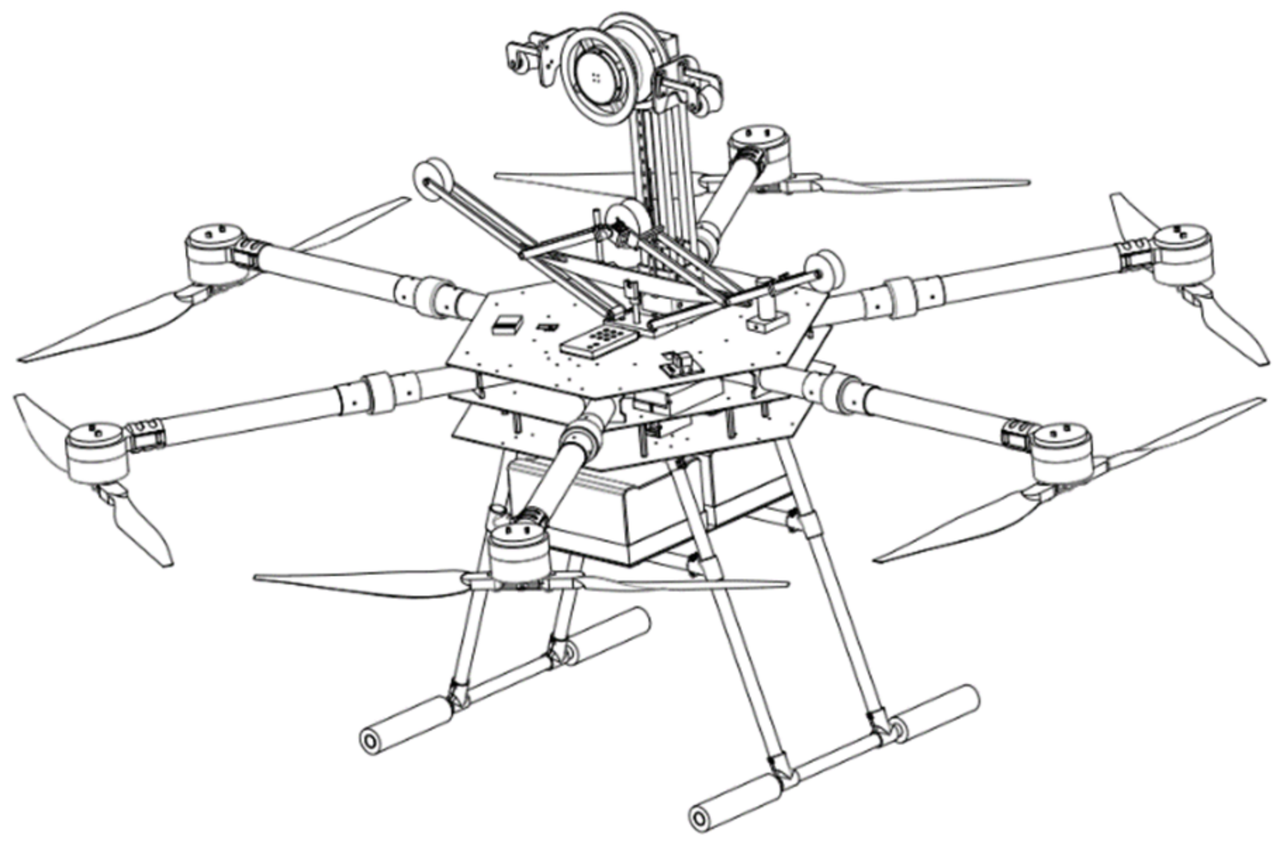
A self-developed FPLIR mainly consists of two parts, a flight mechanism and a walking mechanism, as shown in Figure 1, and the system parameters are listed in

Table 1. Parameters of FPLIR.

Types	Description	Value
FPLIR design parameters	Mass, m/kg	38
	Dimensions, L × W × H/m	1.76 × 1.76 × 1.1
	Distance from rotor center to fuselage center, r/m	0.88
FPLIR model parameters	Body x-axis moment of inertia, $I_x$/kg·m2	5.8
	Body y-axis moment of inertia, $I_y$/kg·m2	5.8
	Body z-axis moment of inertia, $I_z$/kg·m2	8.5
	Atmospheric drag coefficient, $k_f$	1.6865 × 10–6
	Rotor torque coefficient, $k_c$	2.9250 × 10–8

. The flight mechanism adopts an X-type structural design, and six rotor motors with serial numbers M1~M6 are distributed around the center bin. The walking mechanism includes a main traveling wheel, an auxiliary traveling wheel, a main compression wheel, an auxiliary compression wheel, a compression motor, a screw, an encoder, etc.

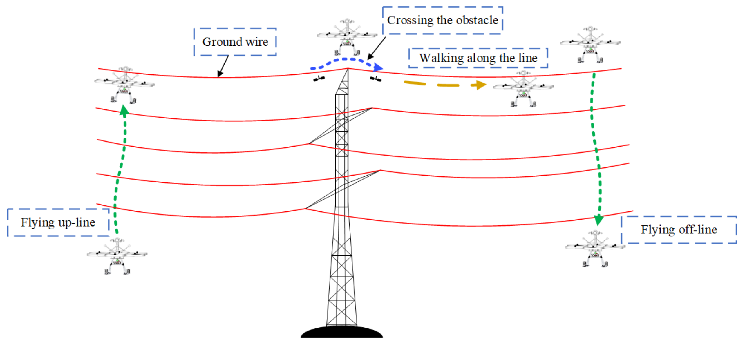
Figure 2 shows the working principle of the robot, where it lifts off the ground to approach the power line and then precisely lands on the line and switches to walking mode to begin the line inspection. When the task is completed, the robot lifts off the line in flying mode. Table 1 shows that the FPLIR has a large mass, volume, and rotational inertia, which require a large minimum turning radius. Since the flight path of the robot is obstructed by the power line during ascent and descent, the reference path inevitably contains multiple corners and line shapes. Power lines are densely distributed, and in order to maintain safety when approaching them, higher requirements are placed on the path-following accuracy of the landing. When the robot has finished inspecting the entire section of the power line, it switches from the walking mode to the flying mode to fly over obstacles. It then repeats the above process. Given the flexible cable structure of the power line, if the robot takes off from a power line with a large following error or slow error convergence, the robot may collide with the power line and cause an accident. Therefore, it is important to carry out path-following research that allows the robot to work under such conditions. To address the mentioned issues concerning the robot’s large turning radius, substantial following error, and slow convergence during path following, an adaptive acceptance circle strategy is proposed. This strategy considers the performance the constraints of the UAV and the reference path information. When the path angle is small, a larger acceptance circle is used, and reference path switching is performed in advance to avoid problems with slow convergence and large overshoot after path switching. If the path angle is large, a smaller acceptance circle is used to make the robot better fit the following path. During the process of following the 3D path, a heading-scaling factor is introduced to regulate the control volume. The spatial distribution of power lines is taken into account to adjust the robot’s priority for its plane path and altitude. This ensures that higher-priority path following is completed more quickly and increases the convergence speed of the UAVs.

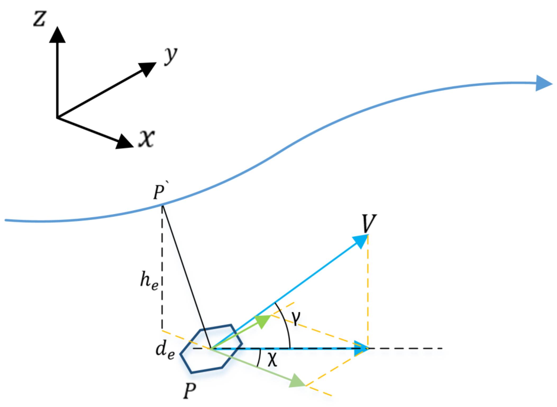
Figure 3 shows the position of the robot relative to the reference path in the inertial coordinate system, xyz. The variable V is the flight velocity; $V_{\widehat{r}}$ is the projected velocity in the horizontal plane; $\gamma$ and $\chi$ are the heading angle and the path inclination, respectively; P is the position of the robot; and $P^{`}$ is the projected point of the robot in the path segment. $d_e$ and $h_e$ are the horizontal and vertical errors of the robot to the projected point, $P^{`}$. The robot path-following control objective is as follows: to design a following control law so that the following error, $\epsilon ={\left[\begin{array}{cc}{d}_e& h_e\end{array}\right]}^T$, satisfies $\underset{t\to \infty }{\mathit{lim}}{d}_e=0$ and $\underset{t\to \infty }{\mathit{lim}}{h}_e=0$. Then, the robot can accurately follow the reference path.

The kinematics of the robot in 3D is modeled as follows:

$$\left\{\begin{array}{c}\begin{array}{c}\dot{x}=Vcos\gamma cos\chi \\ \dot{y}=Vcos\gamma sin\chi \\ \dot{z}=Vsin\gamma \end{array}\\ \begin{array}{c}\dot{V}=\frac{a_x}{cos\chi cos\gamma }\\ \dot{\chi }=\frac{a_y}{Vcos\gamma }\\ \dot{\gamma }=\frac{a_z}{V}\end{array}\end{array}\right.$$

(1)

where (x, y) is the horizontal position of the robot, z is the flight altitude, and γ and χ are the heading angle and path inclination.

3. Path-following Control Based on Improved LOS

3.1. Traditional LOS

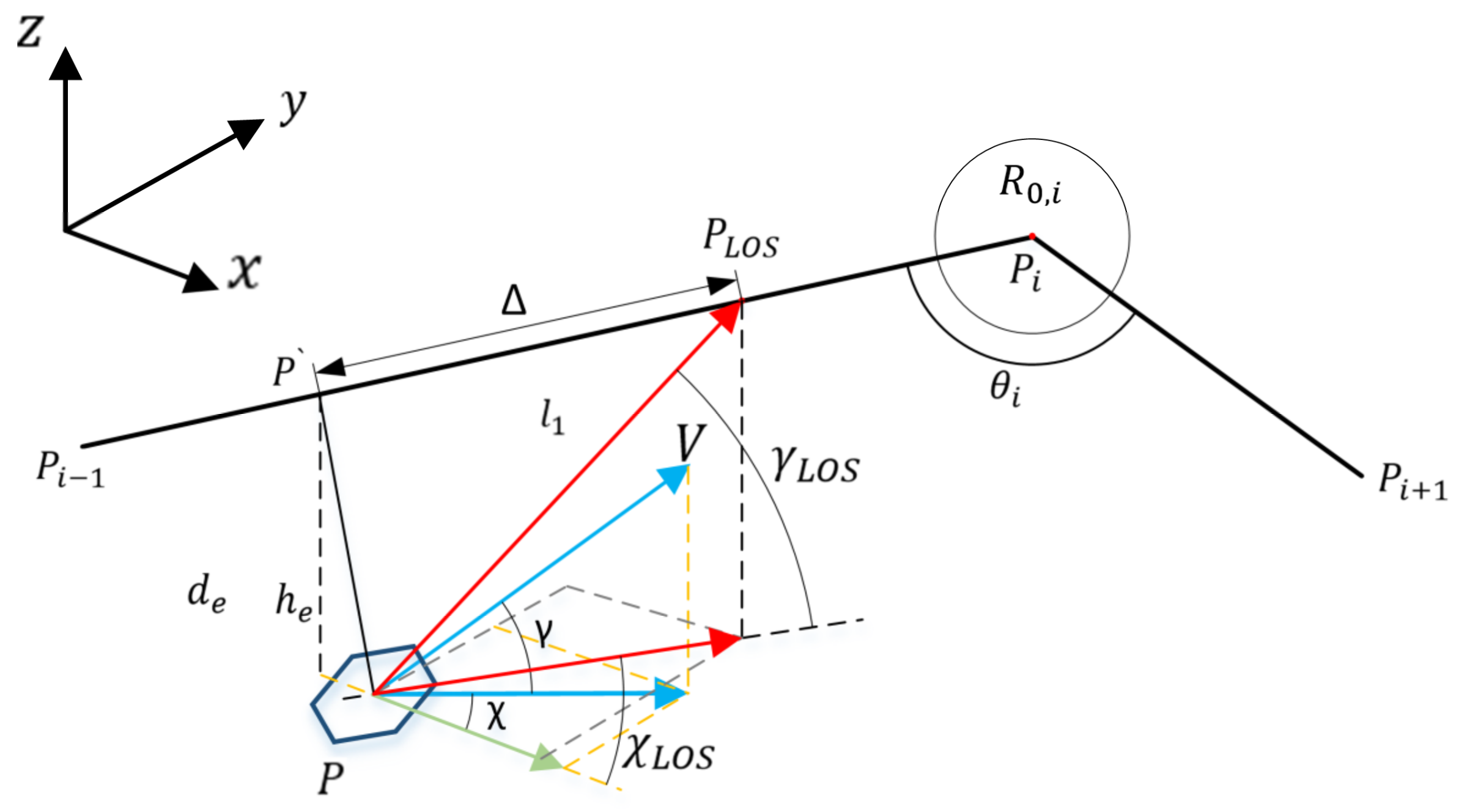
The LOS method is designed to steer a controlled object toward a specific point on a path and then continue to move toward the next point while following it. This method is widely applied in path following and precision guidance. In the traditional LOS method, a fixed acceptance circle is used to efficiently follow the reference path. However, when the reference path segment changes, the fixed acceptance circle can hinder accurate following and slow down convergence speed. The following strategy of the LOS method is depicted in Figure 4:

In Figure 4, $P_{i-1}{P}_i$ is the current following path segment; V is the flight speed; $P_{LOS}$ is the position of the reference point of LOS; P is the position of the robot; $P^{`}$ is the projected position of the robot on the path segment;$\mathsf{\Delta }$ is the forward-looking distance; $R_{0,i}$ is the radius of the acceptance circle of the trajectory point; and ${\gamma }_{LOS}$ and ${\chi }_{LOS}$ are the demand heading angle and the demand trajectory inclination, respectively.$P=(P_1,P_2,\dots ,P_i,\dots P_n)$ is a set of planning path reference points, where each path point has a serial number in the lower right corner, and the points are connected by straight lines.

On the path segment $P_{i-1}{P}_i$, the position of the reference point, $P_{LOS}$, can be found using the following relationship:

$$\left\{\begin{array}{l}{\left(x_{\mathrm{L}\mathrm{O}\mathrm{S}}-x_p\right)}^2+{\left(y_{\mathrm{L}\mathrm{O}\mathrm{S}}-y_p\right)}^2+{\left(h_{\mathrm{L}\mathrm{O}\mathrm{S}}-z_p\right)}^2={\mathsf{\Delta }}^2\\ \frac{x_{\mathrm{L}\mathrm{O}\mathrm{S}}-x_{i-1}}{x_i-x_{i-1}}=\frac{y_{\mathrm{L}\mathrm{O}\mathrm{S}}-y_{i-1}}{y_i-y_{i-1}}=\frac{h_{\mathrm{L}\mathrm{O}\mathrm{S}}-h_{i-1}}{h_i-h_{i-1}}\end{array}\right.$$

(2)

Switch the reference path segment from $P_{i-1}{P}_i$ to $P_i{P}_{i+1}$ as the robot converges to path point $P_i$. This should be done when the distance between the robot and path point $P_i$ satisfies the following condition:

$$\left|P_{ }-P_i\right|⩽R_{0,i}$$

(3)

The robot switches to following the next segment of the path as the reference path segment changes. To achieve the fast following of the reference path, the traditional LOS method employs a fixed acceptance circle. However, if the reference path segment changes, the fixed acceptance circle will affect the convergence speed and the following error for different path angles and flight speeds.

3.2. Improved LOS

To reduce path following error and improve convergence speed, while taking into account the effects of the minimum turning radius, the flight speed, and the angle between the path segments, the acceptance circle in the method must be adaptively adjusted based on the angle of the path segments and the following error. This avoids situations of switching lagging or premature switching when the reference path is changed, which can cause an increase in the path-following error and a slower convergence speed. Therefore, a turning radius threshold is set based on the segment angle and the flight speed of the robot during switching to establish a correspondence between the acceptance circle radius, $R_{0,i}$; the path segment angle, $\theta$; and the flight speed V. This reduces the path-following error and improves the convergence speed.

The principle of the adjustment is as follows:

When $\theta \in (0,\mathsf{\pi }/2)$, the robot switches the path segment with a larger acceptance circle radius. The robot tracks the position of the reference point in the next path segment beforehand and adjusts the heading angle and trajectory inclination to avoid the increased following error due to the delay in switching the reference path segment. When $\theta \in (\mathsf{\pi }/2,\mathsf{\pi })$, a smaller acceptance circle radius is required to follow the reference path to avoid the incomplete following of the previous path segment due to switching the reference path too early.

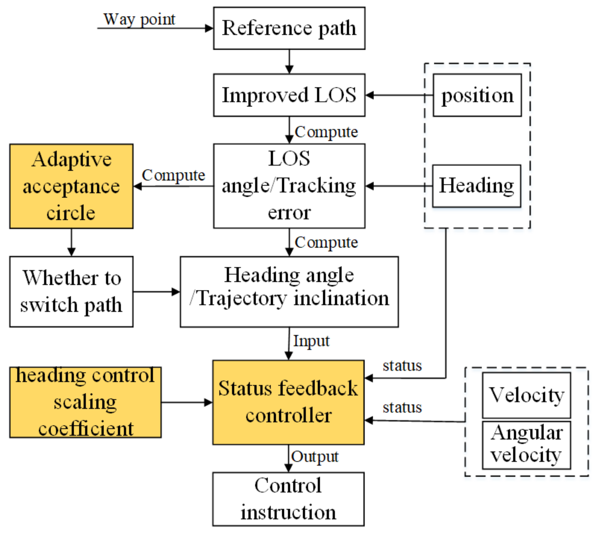
The path-following method includes a navigation subsystem and a control subsystem. The navigation subsystem calculates the path-following error based on the improved LOS, while the control subsystem computes the control command to implement the path-following control based on the output of the navigation subsystem. Scaling coefficients are introduced to adjust the following priorities of parallel and vertical paths for the control commands of the navigation subsystem. The following error is quickly eliminated, and a high-precision path-following effect is obtained.

This paper investigates the adaptive admittance circle and adaptive heading control to reduce the path-following error and accelerate the convergence speed, taking into account the UAV’s maneuvering performance constraints and following path information.

During path following, the following error changes, while the reference point is determined by the forward-looking distance. When the reference point is in the next segment of the reference path, the radius of the admittance circle at the current corner is calculated based on the size of the corner and the current speed. When the UAV is inside the acceptance circle, the reference path segment is switched, and the next closed-loop control begins.

Algorithm 1 shows the operation logic of the improved LOS method:

Algorithm 1: Improved LOS

#The forward control vector, $n^t$, is continuously adjusted based on the distance from the robot’s position, P, to the path in order to achieve the fast convergence of the robot’s trajectory. function PathFollowing  #Calculate the path segment on which the reference point, $P_{LOS}$, is located: $P_{i-1}{P}_i$$/P_i{P}_{i+1}$ $$\begin{gathered} \hspace{1em}\mathbf{While} \mathbf{i} \mathbf{<} \mathbf{n} \mathbf{do} \\ \hspace{1em}\hspace{1em}(n_{\perp }^t,n_{\parallel }^t)⟸\mathrm{C}\mathrm{o}\mathrm{n}\mathrm{s}\mathrm{t}\mathrm{r}\mathrm{u}\mathrm{c}\mathrm{t}\mathrm{V}\mathrm{e}\mathrm{c}\mathrm{t}\mathrm{o}\mathrm{r}\left(\right); \end{gathered}$$ $\hspace{1em}\hspace{1em}{\theta }_d⟸\mathrm{T}\mathrm{h}\mathrm{e}\mathrm{o}\mathrm{r}\mathrm{y}\mathrm{F}\mathrm{o}\mathrm{r}\mathrm{w}\mathrm{a}\mathrm{r}\mathrm{d}\mathrm{D}\mathrm{i}\mathrm{r}\mathrm{e}\mathrm{c}\mathrm{t}\mathrm{i}\mathrm{o}\mathrm{n}\mathrm{A}\mathrm{n}\mathrm{g}\mathrm{l}\mathrm{e}\left(n^t\right)$$; (\#{\theta }_d$ is theoretical angle) $\hspace{1em}\hspace{1em}\theta ⟸\mathrm{A}\mathrm{c}\mathrm{t}\mathrm{u}\mathrm{a}\mathrm{l}\mathrm{A}\mathrm{n}\mathrm{g}\mathrm{l}\mathrm{e}\left(\right);$(# Real angle) $\hspace{1em}\hspace{1em}u⟸\mathrm{S}\mathrm{t}\mathrm{a}\mathrm{t}\mathrm{e}\mathrm{F}\mathrm{e}\mathrm{e}\mathrm{d}\mathrm{b}\mathrm{a}\mathrm{c}\mathrm{k}\mathrm{C}\mathrm{n}\mathrm{t}\mathrm{r}\mathrm{o}\mathrm{l}\left({\theta }_d,\theta \right)$;   # The mass center arrives at the end neighborhood and then moves to the next control segment. The next control phase starts when $P_{LOS}\in P_i{P}_{i+1.}$ $\hspace{1em}\hspace{1em}{R}_{0,i}⟸\mathrm{A}\mathrm{d}\mathrm{m}\mathrm{i}\mathrm{s}\mathrm{s}\mathrm{i}\mathrm{o}\mathrm{n}\mathrm{R}\mathrm{a}\mathrm{d}\mathrm{i}\mathrm{u}\mathrm{s}\mathrm{C}\mathrm{a}\mathrm{l}\mathrm{c}\mathrm{u}\mathrm{l}\mathrm{a}\mathrm{t}\mathrm{e}(R_0,{\theta }_i)$;           if $P\in (R_{0,i},P_i)$ then $\hspace{1em}\hspace{1em}{P}_{i-1}⟵P_i, P_i⟵P_{i+1}$;         end if  return $(n^t$, u);  end while end function

Figure 5 shows the process of path following using the improved LOS method:

As shown in Figure 4 and Figure 5, when entering the acceptance circle of the corner along the path segment, the following approach will be employed to switch to the next path segment:

(1)

Assess whether the FPLIR enters the vicinity of the acceptance circle radius of the corner.

(2)

If it does enter the vicinity, update the current following path segment, and update the projection point, $P^{`}$, of the FPLIR position, P, within the new path segment.

(3)

Based on the forward-looking distance, $\mathsf{\Delta }$, locate a new target point, $P_{LOS}$, on the new path segment starting from the projection point, $P^{`}$.

(4)

Calculate and update the following angle and following inclination according to the new target point, $P_{LOS}$.

(5)

Calculate the control volume according to the new following angle and following inclination.

3.2.1. Adaptive Acceptance Circle Strategy

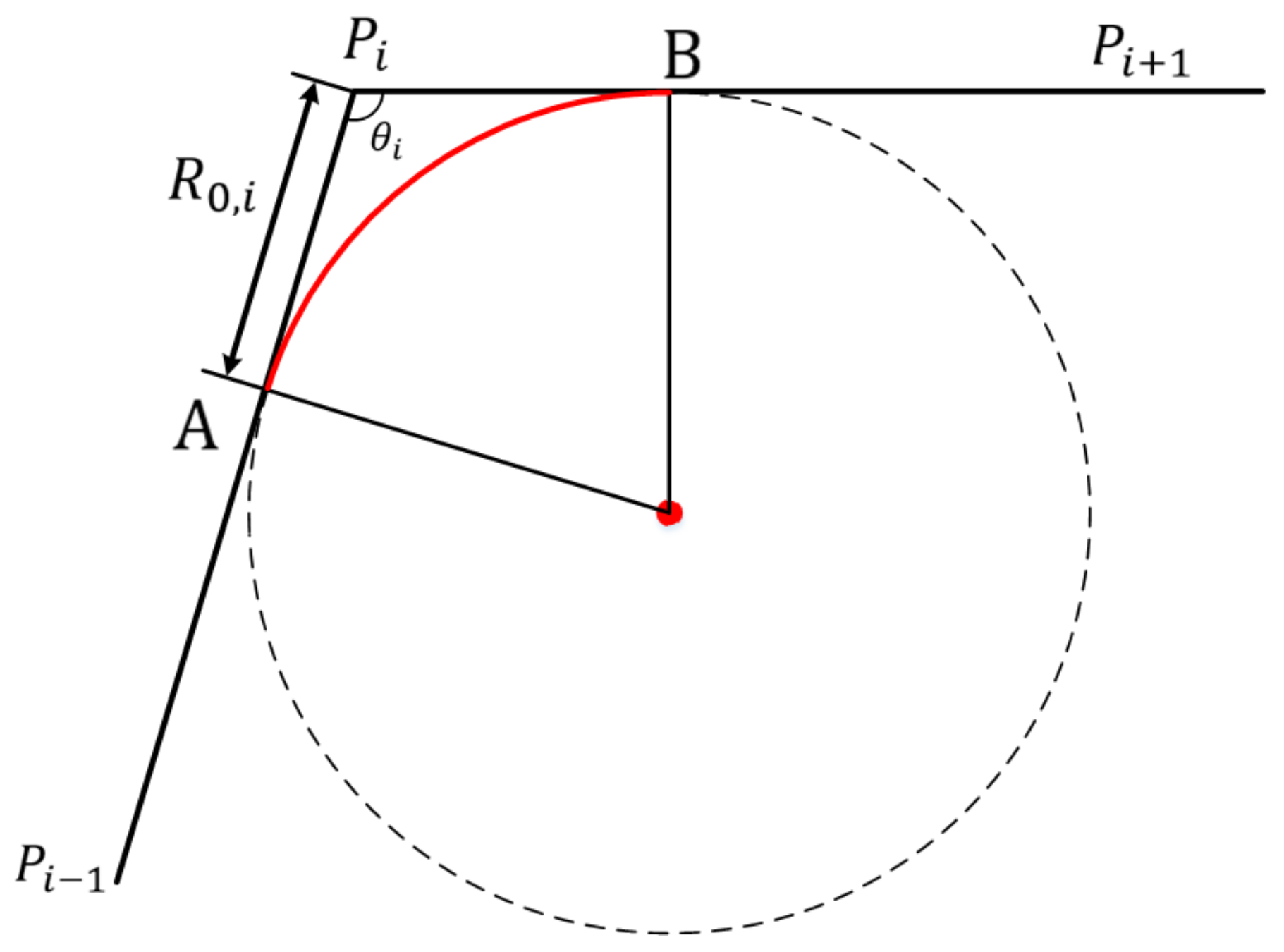
The turning radius of the robot is related to the flight speed during the path change, and the minimum turning radius is determined by the design parameters of the robot itself. As shown in Figure 6, given the minimum turning radius, $R_{min}$, and path angle, ${\theta }_i$, the robot must change its direction at point A by switching from path segment $P_{i-1}{P}_i$ to $P_i{P}_{i+1}$. If the reference turning radius of the robot at point $P_i$ is R, then the radius of the admittance circle at $P_i$ is

$$R_{0,i}=R+k·sigmoid(a·V+b·{\theta }_i)$$

(4)

where $a$ and $b$ are, respectively, the coefficients of velocity and the angle of rotation. If the reference turning radius, $R=R_o$, is set to reduce the following error, when the path angle is $\theta \in (\mathsf{\pi }/2,\mathsf{\pi })$, the following error will oscillate with an increase in $\theta$. To solve this problem, an angular threshold is defined to adjust the acceptance circle radius based on the path segment angle and the current speed.

Considering the correspondence between the radius of the acceptance circle; the angle of the path segment, ${\theta }_i$; and the current velocity, V, the adaptive acceptance circle is designed as follows:

$$\begin{gathered} R_{0,i}=\mathrm{m}\mathrm{a}\mathrm{x}\left\{\begin{array}{c}{R}_0+k·sigmoid(a·V+b·{\theta }_{it})\\ R_{min}\end{array}\right. \\ sigmoid\left(x\right)=\frac{2}{1+e^{-x}}-1 \\ {\theta }_{it}=\mathsf{\pi }-2\mathrm{*}{\theta }_i \\ {\forall \theta }_i\in \left(0,\mathsf{\pi }\right],\mathrm{i}=\mathrm{1,2},\cdots ,\mathrm{n} \end{gathered}$$

(5)

where $R_0$ is the standard acceptance circle radius, which represents the acceptance circle radius in straight flight, and ${\theta }_i$ is the angle in waypoint $P_i$. Parameter k is the scaling factor.

The following can be deduced from Equation (5), which shows the adaptive acceptance circle radius.

If $R_0+k·sigmoid(a·V+b·{\theta }_{it})>R_{min}$, $R_{0,i}$ is set to $R_{0,i}$=$R_0+k·sigmoid(a·V+b·{\theta }_i)$ and the robot completes the turn using the reference turn radius determined by the path segment angle and the current velocity. This is done to prevent following error oscillation.

If $R_0+k·sigmoid\left(a·V+b·{\theta }_{it}\right)\le R_{min}$, $R_{0,i}$ is set to $R_{0,i}=R_{min}$. The robot completes the turn with the minimum turning radius, which can effectively reduce the following error.

3.2.2. Adaptive Heading Control Strategy

The traditional LOS follows the current path by calculating the heading angle and tilt error based on the position error and then calculates the control volume. However, the adjustment time and following distance of this method are long for large position errors. To address this issue, an adaptive heading control strategy is proposed in this paper. This strategy introduces a scaling coefficient to adjust the priority of parallel and vertical paths based on the distance relationship between the robot and the path. To achieve fast, stable, and accurate path following, this paper addresses the problem of large path-following errors and slow convergence speeds to achieve fast, stable, and accurate path following.

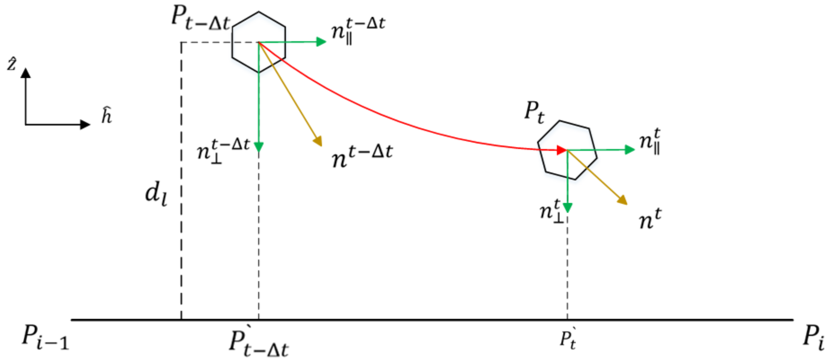
Figure 7 presents the adaptive heading control strategy. In this strategy, $P_{i-1}{P}_i$ is the current path segment for following, $P_i(x_i,y_i,z_i)$ is the coordinates of the path point, P is the position of the robot, and $P^{`}$ represents the robot’s projected position on the path segment.

In Figure 7, the vector $n^t$ corresponds to the direction of the velocity, $V$. As shown in Figure 4, the velocity of the robot can be decomposed into $Vcos\gamma$ components in the horizontal direction and $Vsin\gamma$ components in the vertical direction. Additionally, the $Vcos\gamma$ component in the horizontal direction can be further decomposed into x-axis and y-axis components based on the trajectory inclination.

The adaptive heading control strategy in this paper introduces a scaling coefficient, m, to regulate the priority between vertical and horizontal following exclusively while not interfering with the vector components in the x-axis direction and y-axis direction components within the horizontal following. Therefore, a 2D coordinate system, $\widehat{z}-\widehat{h}$, composed of horizontal and vertical axes is employed.

As shown in Figure 7, the workflow of the velocity control strategy for each path segment of the robot in the xoy plane is as follows:

(1)

The start and end points of the current path segment are designated as $P_{i-1}$ and $P_i$, respectively. The robot’s path following involves closed-loop control of the current path segment. The next path segment is then controlled in a similar way.

(2)

The point P represents the robot’s centroid. $P^{`}$ is defined as the projection of P onto the linear path. $d_l$ refers to the distance between the robot and the planned path.

(3)

The vector $n^t$ represents the forward direction of the robot at time t. The vector $n_{\parallel }^t$ is the parallel projection of $n^t$ onto the segment $P_{i-1}{P}_i$, while $n_{\perp }^t$ is the orthogonal vector to $n_{\parallel }^t$, thus representing the vertical vector of the segment, $P_{i-1}{P}_i$.

(4)

The letter m is defined as the scaling coefficient of the distance, $d_l$, between the robot centroid, P, and the planned path; thus, the forward direction vector of the control robot is

$$n^t=\frac{m{d}_l}{1+m{d}_l}{n}_{\perp }^t+\frac{1}{1+m{d}_l}{n}_{\parallel }^t$$

(6)

Equation (6) shows that if the value of the scaling coefficient m is close to 0, the coefficient of $n_{\perp }^t$ approximates to 0 while the coefficient of $n_{\parallel }^t$ approximates to 1. This causes the robot to advance in the direction parallel to the path. Conversely, if the scaling coefficient, m, is close to ∞, the robot advances in the vertical direction to the path. Altering parameter m provides different path-following priorities. To facilitate analysis, Equation (6) can be rewritten as follows:

$$n^t=\frac{1}{1+\frac{1}{m{d}_l}}{n}_{\perp }^t+\frac{1}{1+m{d}_l}{n}_{\parallel }^t$$

(7)

At a greater distance from the planning path, the value of $d_l$ increases, causing the scaling coefficient of $n_{\perp }^t$ to exceed that of $n_{\parallel }^t$. As a result, the robot moves along the vertical direction. When the robot approaches the planning path, the value of $d_l$ decreases so that the scaling coefficient of $n_{\perp }^t$ is less than that of $n_{\parallel }^t$. As a result, the robot moves along the parallel direction. During the control segment of $P_{i-1}{P}_i$, control vector $n^{t-\Delta t}$ at time $t-\mathsf{\Delta }t$ transitions into control vector $n^t$ at moment t. The control direction gradually aligns with the forward direction of the path of $P_{i-1}{P}_i$, resulting in the gradual convergence of the position error and the direction error to zero. This ensures the rapid convergence of the robot along the planned path.

3.2.3. Design of the State-Feedback-following Controller

The control system for path following consists of a navigation subsystem and a control subsystem. The path following error is obtained by the navigation subsystem based on the improved LOS. The control subsystem then obtains the control command based on the output of the navigation subsystem in order to realize the path-following control. Considering the projected point, $P^{`}$, and the reference path point, $P_{LOS}$, the LOS path following error, $e={[d_e,h_e,{\psi }_e,{\gamma }_e]}^T$, can be defined. 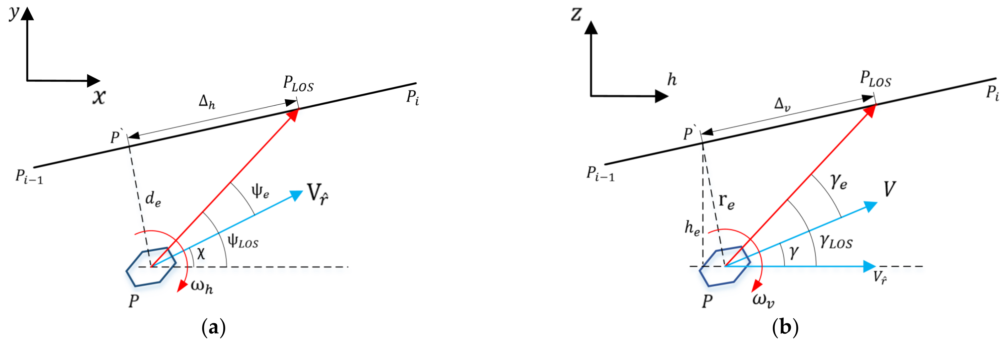${\mathsf{\omega }}_{\mathrm{h}}$ and ${\mathsf{\omega }}_{\mathrm{v}}$ are horizontal and vertical angular velocity, respectively. Based on the following error, the path-following control law is designed. The following schematic diagrams in the horizontal plane and in the vertical plane are shown in Figure 8a and Figure 8b, respectively.

The following error in the horizontal plane, $e_h={{[d}_e,{\psi }_e]}^T$, is defined as follows:

$$\left\{\begin{array}{l}{d}_{\mathrm{e}}=\sqrt{{\left(x_p-x\right)}^2+{\left(y_p-y\right)}^2}=\sqrt{e_x^2+e_y^2}\\ {\psi }_{\mathrm{e}}={\psi }_{\mathrm{L}\mathrm{O}\mathrm{S}}-\chi =\mathrm{a}\mathrm{r}\mathrm{c}\mathrm{t}\mathrm{a}\mathrm{n}\left(\frac{y_{los}-y}{x_{los}-x}\right)-\chi \end{array}\right.$$

(8)

The differential equation for the following error can be obtained from Equation (8) as

$$\left\{\begin{array}{l}{\dot{d}}_{\mathrm{e}}=V_{\widehat{r}}\mathrm{s}\mathrm{i}\mathrm{n}{\psi }_{\mathrm{e}}\\ {\dot{\psi }}_{\mathrm{e}}=\frac{1}{1+{\left(\frac{y_{los}-y}{x_{los}-x}\right)}^2}-{\omega }_{\mathrm{h}}\end{array}\right.$$

(9)

where $x_{los}$ and $y_{los}$ are the projected coordinates of the horizontal plane.

The acceleration command using the linearization assumption and state feedback method for the robot is designed as follows:

$$a_y^{\mathrm{c}}=-V_{\widehat{r}}\left(k_1{d}_{\mathrm{e}}+k_2{\psi }_{\mathrm{e}}\right)$$

(10)

where $V_{\widehat{r}}=Vcos\gamma$ is the component of velocity in the horizontal plane.

The following error in the vertical plane, $e_h={{[d}_e,{\psi }_e]}^T$, is defined as follows:

$$\left\{\begin{array}{l}{h}_{\mathrm{e}}=h_p-h\\ {\gamma }_{\mathrm{e}}={\gamma }_{\mathrm{L}\mathrm{O}\mathrm{S}}-\gamma =arctan\left(\frac{z_{los}-z}{h_{los}-h}\right)-\chi \end{array}\right.$$

(11)

The differential equation for the following error can be obtained from Equation (11) as follows:

$$\left\{\begin{array}{l}{\dot{h}}_{\mathrm{e}}=V\mathrm{s}\mathrm{i}\mathrm{n}\gamma \\ {\dot{\gamma }}_{\mathrm{e}}=\frac{1}{1+{\left(\frac{z_{los}-z}{h_{los}-h}\right)}^2}-{\omega }_v\end{array}\right.$$

(12)

where $h_{los}$ and $z_{los}$ are the projected coordinates of the vertical plane.

Similarly, the acceleration command for the robot’s vertical acceleration command can be derived as follows:

$$a_z^c=-V{k}_3{\gamma }_{\mathrm{e}}$$

(13)

Thus, the control instructions for the 3D path following of robot are as follows:

$$\left\{\begin{array}{l}{a}_y^{\mathrm{c}}=-V_{\widehat{r}}\left(k_1{d}_{\mathrm{e}}+k_2{\psi }_{\mathrm{e}}\right)\\ a_z^c=-V{k}_3{\gamma }_{\mathrm{e}}\end{array}\right.$$

(14)

The pole configuration method can select following control laws (10) and (13) based on the state feedback design with a feedback gain matrix, $\mathrm{k}=[k_1,k_2,k_3]$, to ensure the stability of the following closed-loop system. In the pole configuration, the system is designed to achieve the expected damping ratio and control time, thereby avoiding the oscillation of the error curve and ensuring fast convergence. The stability of the following control system is demonstrated using the following error in the horizontal plane as an example. The linear error system is expressed as follows:

$$\dot{e}=Ae+Bu$$

(15)

The state matrix, A, and the input matrix, B, are defined as follows:

$$\mathrm{A}=\left[\begin{array}{cc}-\frac{V_{\widehat{r}}}{\mathsf{\Delta }}& V_{\widehat{r}}\\ 0& \frac{V_{\widehat{r}}}{\mathsf{\Delta }}\end{array}\right], \mathrm{B}=\left[\begin{array}{c}0\\ 1\end{array}\right]$$

(16)

The control quantity designed based on the state feedback is denoted by u:

$$u=-Ke$$

(17)

where K represents the feedback gain matrix.

As a result, the equation for the closed-loop system is

$$\dot{e}=(A-BK)e$$

(18)

In the above equation, the characteristic polynomial of the system’s closed-loop equation is

$$\left|sI-A+BK\right|=(s-p_1)(s-p_2)$$

(19)

During the pole configuration process, $p_1$ and $p_2$ are chosen as negative roots with conjugate complex values to determine the damping ratio and control time of the system. Since the conjugate complex roots, $p_1$ and $p_2$, are situated on the left half of the s-plane, the closed-loop following system is stable, which serves to prove the overall stability of the system.

4. Simulation Experiments and Analysis

The effectiveness of the adaptive acceptance circle strategy and the adaptive heading control strategy in improving path-following performance is verified through simulation experiments and is compared with the classical line-of-sight method.

During the simulation experiments, the initial position of the robot is $x_0=0$ m, $y_0=5$ m, and $z_0=0$ m. Additionally, the initial heading angle is $\gamma =0°$, and the track inclination angle is $\chi =0°$. A comparative study is conducted based on the traditional LOS method and the improved LOS method proposed in this paper to verify the effectiveness of the adaptive acceptance circle and the adaptive heading control strategy in improving the path-following performance. The radius of the adaptive acceptance circle is taken as the circle shown in Equation (5), where a = 2, b = 1, k = 0.2, and the scaling coefficient of the adaptive heading control is m = 2.5. The control period is T = 0.1 s. In these simulation experiments, three corners are mainly considered, namely, the small corners of the horizontal angle, ${\theta }_a<90°$ and ${\theta }_b<90°$, as well as the larger angle of the horizontal pinch angle, ${\theta }_c>\mathsf{\pi }/2$.

Table 2. Parameters of the simulation experiment.

Parameter/Unit	Value
$\mathrm{Fixed} \mathrm{forward}-\mathrm{looking} \mathrm{distance} \mathsf{\Delta }$/(m)	0.5
$\mathrm{Fixed} \mathrm{acceptance} \mathrm{circle} \mathrm{radius} R_0$/(m)	0.5
Start velocity/(m/s)	0

lists the general parameters for simulation experiment.

4.1. Experiments on Heading Control Strategy

To evaluate the effectiveness of the improved adaptive heading control strategy on path following, we compare its performance with a state feedback control strategy. The comparison is performed using a fixed acceptance circle radius: $R_0=0.5$ m. The results of this experiment show that the new strategy improves the path-following accuracy. The flying speed of the robot was maintained at v = 0.2 m/s during the simulation experiment.

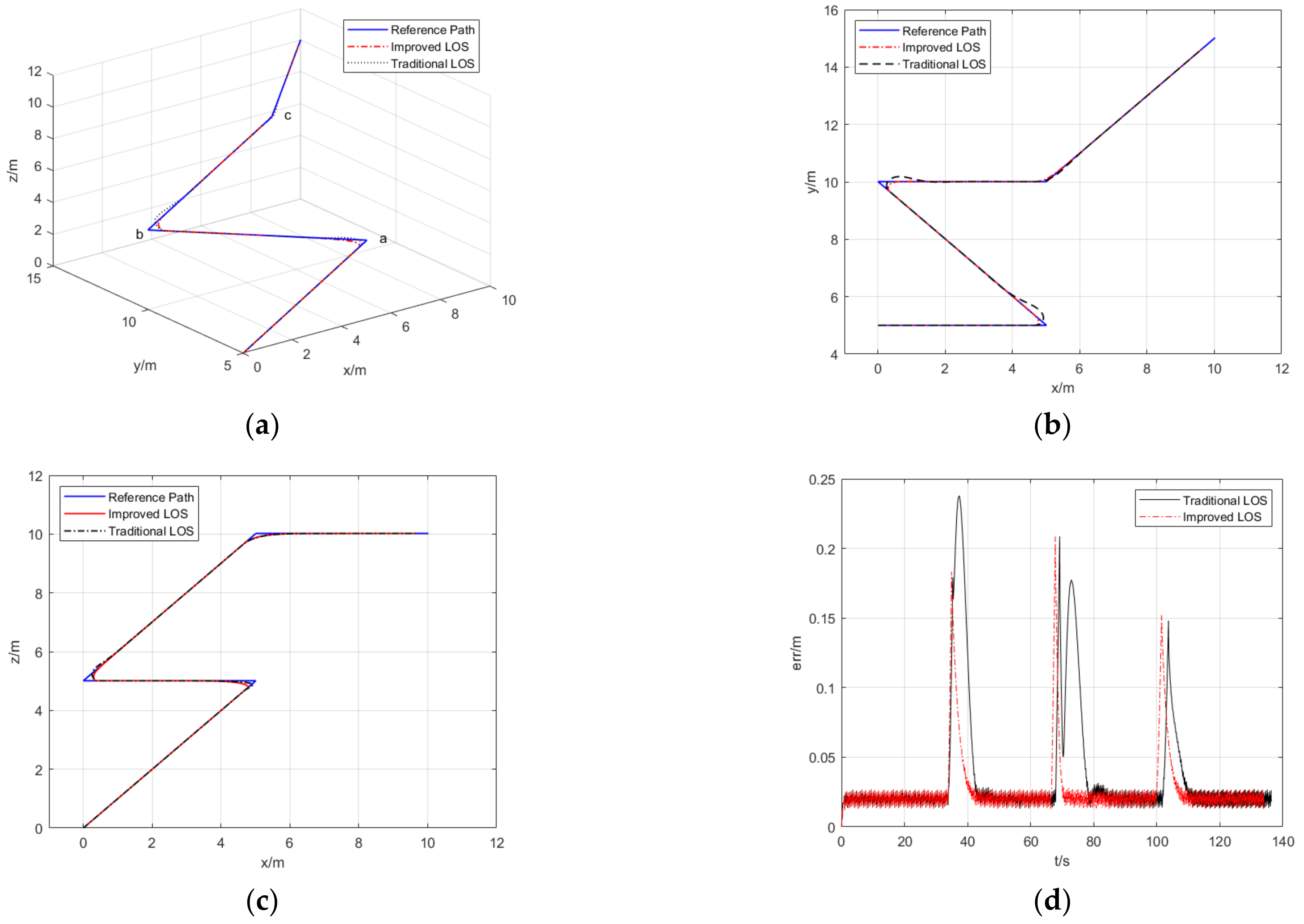
The experimental results are presented in the following figures: Figure 9 shows the 3D path-following results, Figure 9a shows the following trajectory of the 3D path following, Figure 9b shows the xoy plane projection of the 3D path-following trajectory, and Figure 9c shows the xoz plane projection of the 3D path-following trajectory. The simulation results reveal the robot’s ability to execute path following on the reference path under different following methods. Figure 9d shows the following error versus time curve between the robot’s real-time position and the reference path. The abrupt change in the error curve corresponds to the moment it reaches the corner of the reference path. It is worth noting that the oscillations of the following error in Figure 9d are caused by the earlier updating of the error statistics with the $P_{LOS}$ update. The variations in Figure 9d correspond to the path points a, b, and c. As depicted in Figure 9, the following trajectory with the improved LOS is closer to the reference path.

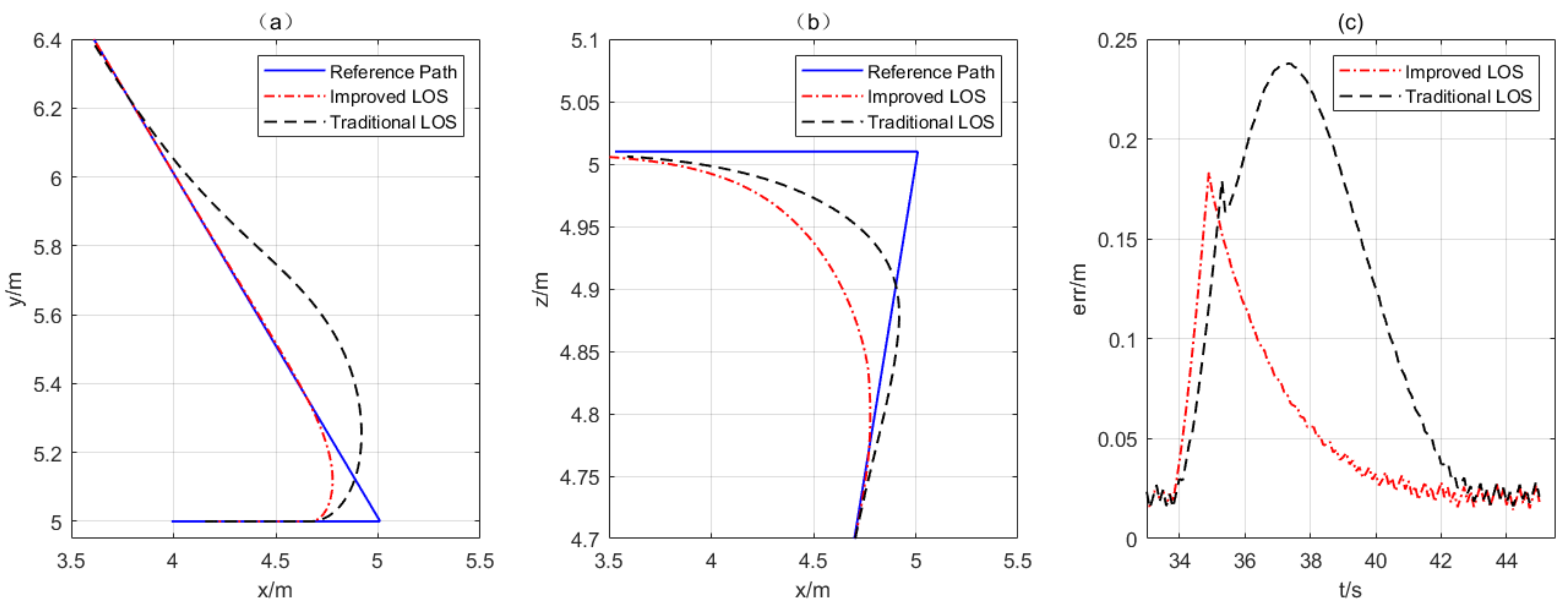
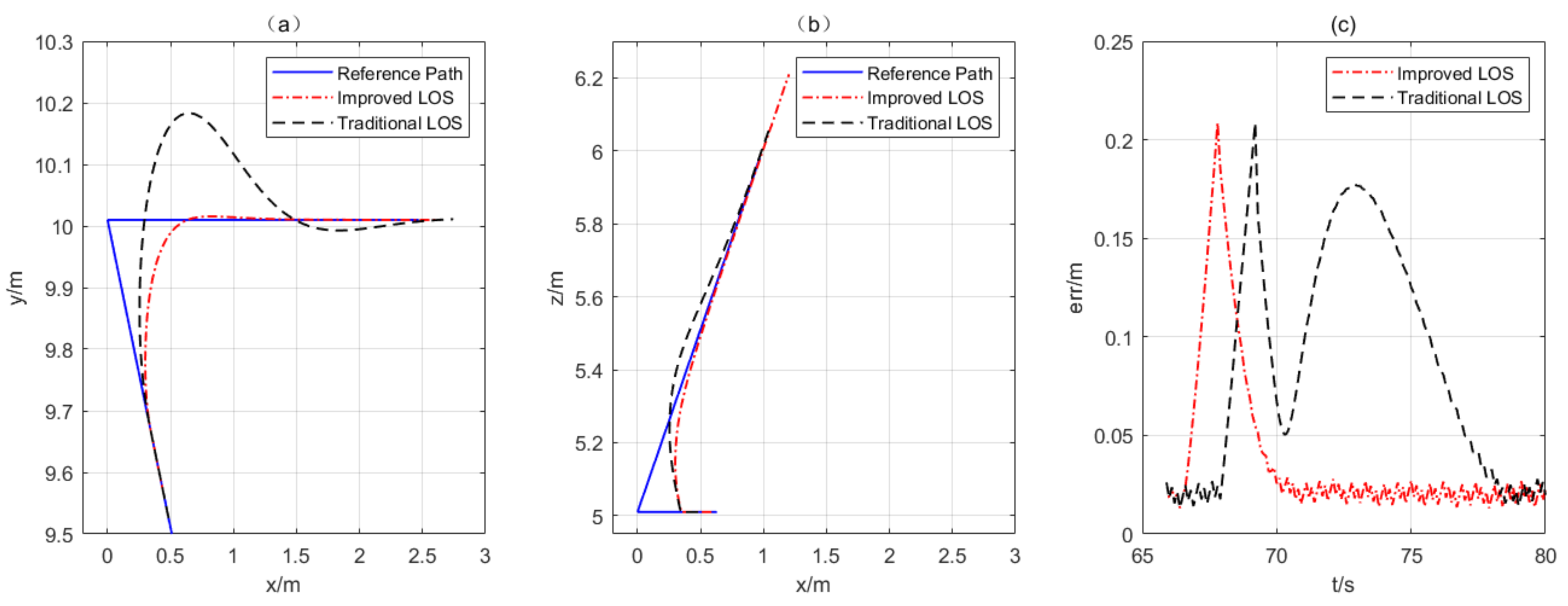
In order to further verify the effect of adaptive heading control on improving path-following accuracy and convergence speed, the details of the horizontal projection, vertical projection, and following error curve of the robot’s following trajectory at points a, b, and c are shown in Figure 10, Figure 11 and Figure 12. The following conclusions can be obtained by analyzing Figure 10, Figure 11 and Figure 12.

(1)

For smaller angles, the adaptive navigation control shows a smaller following error and an improved following effect. At point a, the maximum following error decreases from 0.238 m to 0.183 m, indicating a reduction in the following error of 0.055 m. At point b, there is little or no significant reduction in the maximum following error. At point c, the maximum following error decreases from 0.152 m to 0.148 m, indicating a reduction in the following error of 0.004 m. This improvement also enhances the oscillatory convergence phenomenon.

(2)

The convergence time of the adaptive heading control is faster. At point a, the convergence time is reduced from 8.1 s (from 33.7 s to 41.8 s) to 5.1 s (from 33.7 s to 38.8 s), and the time taken to converge is reduced by 3 s. At point b, the convergence time is reduced from 9.3 s (from 67.9 s to 77.2 s) to 2.8 s (from 66.6 s to 69.4 s), and the time consumed for convergence is reduced by 6.5 s. Similarly, at point c, the convergence time is reduced from 5.8 s (from 102.1 s to 107.9 s) to 4.7 s (from 100.0 s to 104.7 s), and the time taken for convergence is reduced by 1.1 s. Convergence time is determined when the following curve intersects the 5% error margin.

Similarly, an adaptive heading control strategy will provide a much higher approach speed and lower following error, resulting in better control results.

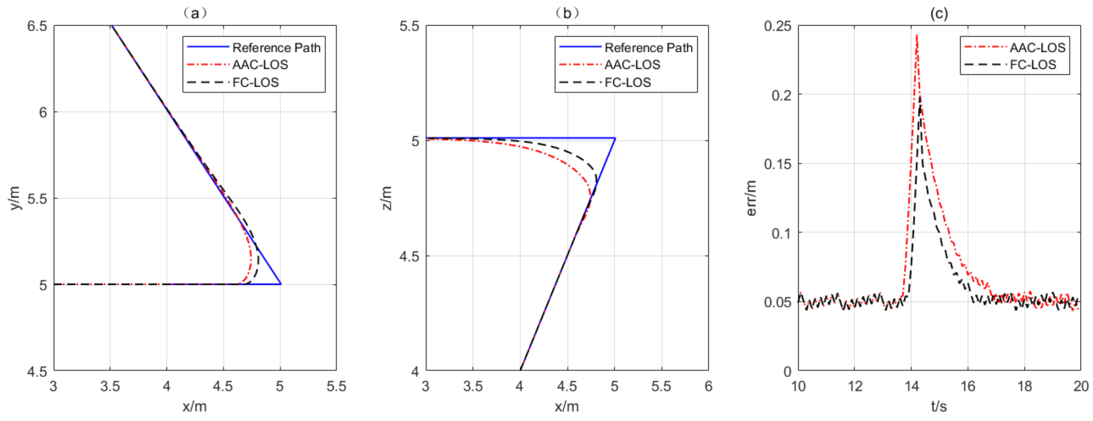
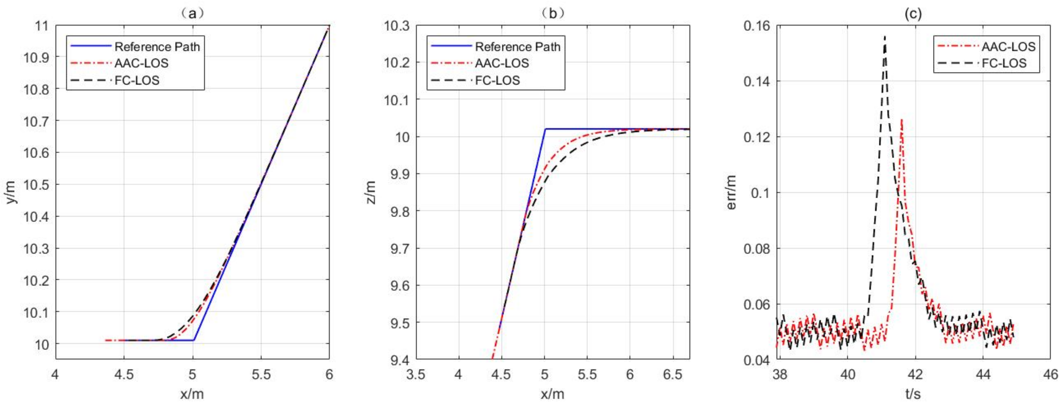
4.2. Acceptance Circle Comparison Experiments

A comparative study is conducted to verify the effectiveness of the adaptive Acceptance circle strategy in improving path-following accuracy. Specifically, FC-LOS (fixed acceptance circle-based LOS), which uses a fixed acceptance circle, is compared with AAC-LOS (adaptive acceptance circle-based LOS). By maintaining a constant following path and applying adaptive heading control, this study compares the following effects of the LOS method using a fixed acceptance circle with the adaptive adjustment acceptance circle strategy. During the simulation experiment, the robot’s flight speed is set at $v=0.5\mathrm{m}/\mathrm{s}$. To maintain a consistent height in the following state, the height of following is increased to a fixed height. The path-following paths of the path angles ${\theta }_a<\pi /2$ at point a and ${\theta }_c>\pi /2$ at point c are selected as the objects of comparison. 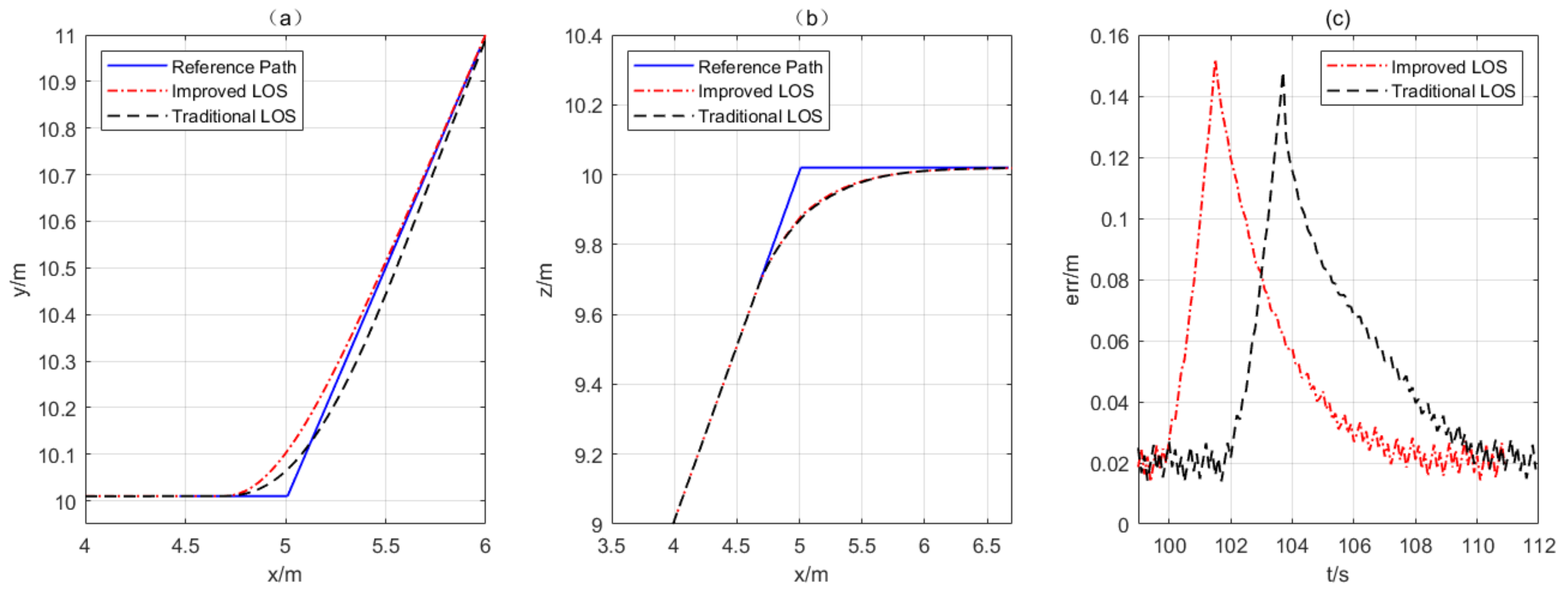Figure 13 and Figure 14 show the experimental results. Figure 13 corresponds to the following results at point a, while Figure 14 corresponds to the following results at point c. After analyzing these figures, the following conclusions can be drawn.

(1)

The adaptive acceptance circle strategy effectively solves the issue of switching ahead or lagging and maintains a controllable following error even when the reference path switches ahead. Figure 13 shows that the following trajectory, based on the adaptive acceptance circle, switches to the reference path segment earlier because of the larger acceptance circle radius, resulting in faster convergence to the next path segment. Figure 14 shows that the following trajectory based on the adaptive acceptance circle switches closer to the reference path because of the smaller acceptance circle radius, resulting in a reduction in the maximum following error from 0.156 m to 0.126 m.

(2)

The convergence of the adaptive acceptance circle strategy is faster. For point a, where ${\theta }_a<\pi /2$, the overall convergence time using AAC-LOS slightly increases compared with FC-LOS, as shown in Figure 13. However, during the xoy path following, the AAC-LOS can follow the reference path faster compared with FC-LOS. For point c, where ${\theta }_c>\pi /2$, as shown in Figure 14, the total convergence time is reduced from 1.4 s (from 40.6 s to 42 s) to 1.4 s (from 41.2 s to 42 s), a reduction of about 0.6 s.

In summary, the adaptive acceptance circle strategy offers more obvious advantages in terms of path-following accuracy and convergence speed.

5. Discussion

5.1. Comparison of Improved LOS and Traditional LOS

Switching following errors are reduced to varying degrees when using the improved LOS method as compared with the traditional LOS method. Additionally, the convergence speed and path-following accuracy are significantly improved. The use of traditional LOS path following with a fixed acceptance circle radius is simple and straightforward and is capable of offering stable and predictable path following in certain application contexts. However, the fixed acceptance circle radius has some limitations: at high speeds, it may cause excessively aggressive path following, whereas at low speeds, it may lead to conservative path following.

The adaptive acceptance circle strategy adjusts the radius of the circle based on the vehicle’s motion. This allows the vehicle to use a smaller radius at the curved region of the path and a larger radius for the larger path corners to fit the path more closely. To better account for the relationship between the vehicle and the following path, it is recommended that a larger circle radius is used at the larger corners and that the following path segments are switched ahead. This enables the vehicle to stay closer to the path, reducing following errors and overshoot.

The traditional LOS method uses heading angle error feedback for control to handle large position deviations. However, the method requires a longer convergence time and following distance. Moreover, the maximum following distance of the robot is restricted by the limited space defined by the segmentation of the power lines. The adaptive heading control strategy uses the scaling coefficient based on the distance between the robot and the path. It adjusts the priority of parallel and vertical path following. As the distance between the robot and the following path increases, the priority of parallel path following also increases. This method can effectively overcome the issues of large following errors and slow convergence speeds, thereby achieving fast, stable, and accurate path following.

The proposed improved LOS method is used to analyze the equation of the 3D path-following error and to design a following control law based on state feedback, with the following error as the control object. Stability analysis is then performed to ensure that the following control law meets the requirements of accuracy and reliability in 3D path following.

5.2. Selection of Experimental Parameters for Improved LOS

This paper presents simulation experiments aimed at simulating the path-following effect of the improved LOS method during robot flight, especially for frequently changing paths. The results of the experiments indicate that the 3D path-following method using the improved LOS method is able to adaptively adjust the size of the acceptance circle radius based on the path angle and the current flight speed of the robot. This allows it to switch reference paths while reducing following error and satisfying the robot’s performance constraints. It is also able to prioritize horizontal and vertical paths based on their real-time distance from the reference paths, guiding the robot toward rapid convergence with the reference paths.

In the simulation experiments on adaptive heading control, the robot’s forward-looking distance is set to 0.5 m at a flight speed of 0.2 m/s. This is because the distance between the phase wire and the ground wire in an environment with power line divisions is usually between 1 and 2 m. When maintaining a safe distance, the robot’s flight envelope becomes narrow; thus, a small forward-looking distance is chosen. Additionally, the robot should follow the planned path at a slower flight speed for robot safety. In the case of the adaptive acceptance circle strategy, the speed and angle of the path segment are weighted at 2 and 1, respectively, with a flight speed of 0.5 m/s. Therefore, when planning of the adaptive acceptance circle, it is expected that the priority of the current flight speed will exceed the angle of the path segment. In order to achieve a higher accuracy of the path-following control, the adaptive heading control strategy adopts a smaller scale coefficient, m, based on the robot’s horizontal error requirements in flight. This increases the priority of horizontal control in the heading control process.

Given the results of simulation experiments, both the improved LOS method and the traditional LOS method are able to effectively follow the preset paths of the robot, and compared with the traditional LOS method, the improved LOS method has faster convergence speed; smaller following errors; and better performance in terms of stability, robustness, and response speed in path following, which is important for improving the flight accuracy and safety of the FPLIR in spaces segmented by power lines.

5.3. Limitations and Future Work

The proposed method has some limitations. Firstly, the method is highly reliant on the selection of parameter m. To achieve optimal path following, different path types and environments may need different values of m. Thus, tests are required to determine the optimal value of m. Secondly, in practical environments, paths may be significantly varied, ranging from straight lines to curves and crossings, among others. Given the experimental results, the method appears proficient in following paths consisting of straight lines, although it may have limitations when dealing with more diverse paths. Additionally, the experiments described in this paper feature a certain level of regularity and specificity in corner size and path design. Although path segments with different angles and flight tasks are designed, it is necessary to increase the variety of tracked paths and further investigate the problem of path following under multiple forms of paths for robots in constrained spaces.

6. Conclusions

This paper analyzes the robot flight environment and different working conditions of the FPLIR. It investigates the problem of 3D path-following control in the restricted space of power lines. In addition, this paper proposes the adaptive acceptance circle strategy and the adaptive heading control strategy. The numerical simulation experiments are carried out, and the following conclusions are drawn:

(1)

Under the condition of a fixed acceptance circle, compared with the traditional LOS method, the average path-following error of the improved LOS method with adaptive heading control is reduced by 0.167 m, and the average convergence time is reduced by 2.05 s for a path angle of $\theta \in (0,\pi /2)$. However, when $\theta \in (\pi /2,\mathsf{\pi })$, the following error remains almost constant, and the convergence time is reduced by 0.6 s. The proposed adaptive heading control strategy significantly improves following accuracy and the convergence speed of the path following, reducing following errors caused by large switching angles and effectively following the reference path.

(2)

When keeping the reference path and the adaptive heading control scale coefficient unchanged, the adaptive acceptance circle strategy improves the problem of switching the reference path too early or lagging behind. This strategy fully follows the reference path and reduces the following error. When the path angle is between $\theta \in (0,\pi /2)$, the following trajectory based on the adaptive acceptance circle switches the reference path segment earlier due to the acceptance circle’s larger radius. However, this increases the following error while maintaining the controllable state and reduces the convergence time by 0.8 s. When the path angle is between $\theta \in (\pi /2,\mathsf{\pi })$, the following trajectory based on the adaptive acceptance circle is closer to the reference path because of the smaller radius. This approach reduces the maximum following error by 0.3 m and the convergence time by approximately 0.4 s, leading to shorter convergence times and smaller following errors.

(3)

Using the improved LOS method, the state feedback path-following control method satisfies the following requirements of convergence, reliability, and accuracy and also has advantages in following accuracy and convergence speed.

(4)

The proposed method is highly reliant on the selection of the scaling coefficient, m, which must be determined via testing under various conditions. The method is effective for following a path consisting of straight lines, but further research is needed to solve the problem of following a path under different types of paths.